Faster and Deterministic Subtrajectory Clustering

Abstract

Given a trajectory $T$ and a distance $\Delta$, we wish to find a set $C$ of curves of complexity at most $\ell$, such that we can cover $T$ with subcurves that each are within Fréchet distance $\Delta$ to at least one curve in $C$. We call $C$ an $(\ell,\Delta)$-clustering and aim to find an $(\ell,\Delta)$-clustering of minimum cardinality. This problem was introduced by Akitaya et al. (2021) and shown to be NP-complete. The main focus has therefore been on bicriterial approximation algorithms, allowing for the clustering to be an $(\ell,\Theta(\Delta))$-clustering of roughly optimal size.

We present algorithms that construct $(\ell,4\Delta)$-clusterings of $\mathcal{O}(k\log n)$ size, where $k$ is the size of the optimal $(\ell,\Delta)$-clustering. For the discrete Fréchet distance, we use $\mathcal{O}(n\ell\log n)$ space and $\mathcal{O}(kn^{2}\log^{3}n)$ deterministic worst case time. For the continuous Fréchet distance, we use $\mathcal{O}(n^{2}\log n)$ space and $\mathcal{O}(kn^{3}\log^{3}n)$ time. Our algorithms significantly improve upon the clustering quality (improving the approximation factor in $\Delta$) and size (whenever $\ell\in\Omega(\log n)$). We offer deterministic running times comparable to known expected bounds. Additionally, in the continuous setting, we give a near-linear improvement upon the space usage. When compared only to deterministic results, we offer a near-linear speedup and a near-quadratic improvement in the space usage. When we may restrict ourselves to only considering clusters where all subtrajectories are vertex-to-vertex subcurves, we obtain even better results under the continuous Fréchet distance. Our algorithm becomes near quadratic and uses space that is near linear in $n\ell$.

1 Introduction

Buchin, Buchin, Gudmundsson, Löffler, and Luo [9] proposed the subtrajectory clustering problem. The goal is to partition an input trajectory $T$ of $n$ vertices into subtrajectories, and to group these subtrajectories into clusters such that all subtrajectories in a cluster have low Fréchet distance to one another. The clustering under the Fréchet distance is a natural application of Fréchet distance and a well-studied topic [16, 12, 11, 10, 17] that has applications in for example map reconstruction [7, 8]. Throughout recent years, several variants of the algorithmic problem have been proposed [9, 1, 3, 6]. Agarwal, Fox, Munagala, Nath, Pan, and Taylor [1] aim to give a general definition for subtrajectory clustering by defining a function $f$ that evaluates the quality of a set of clusters $C$. Their definition, however, does not encompass the definition in [9] and has nuances with respect to [3, 6, 14].

Regardless of variant, the subtrajectory clustering problem has been shown to be NP complete [9, 1, 3]. Agarwal, Fox, Munagala, Nath, Pan, and Taylor [1] therefore propose a bicriterial approximation scheme. They present a heuristic algorithm for the following. Suppose that we are given some $\Delta\geq 0$. Let $k$ denote the smallest integer such that there exists a clustering $C$ with $k$ clusters with score $f(C)\leq\Delta$. The goal is to compute a clustering $C^{\prime}$ with $\mathcal{O}(k\operatorname{polylog}n)$ clusters and score $f(C)\in\Theta(\Delta)$.

Akitaya, Brüning, Chambers, and Driemel [3] present a less general, but more computable, bicriterial approximation problem: suppose that we are given some $\Delta\geq 0$ and integer $\ell\geq 1$. An $(\ell,\Delta)$-clustering is a set $C^{*}$ of clusters (sets of subtrajectories) where

• $C^{*}$ covers $T$: for all points $t$ on $T$, there is a cluster $Z\in C^{*}$ and curve $S\in Z$ containing $t$, and

• every cluster $Z\in C^{*}$ contains a “reference curve” $P_{Z}$ with at most $\ell$ vertices, and

• for every $Z\in C^{*}$, all subtrajectories $Q\in Z$ have $d_{F}(P_{Z},Q)\leq\Delta$.

Under the discrete Fréchet distance, they compute an $(\ell,19\Delta)$-clustering $C$ of $\mathcal{O}(k\ell^{2}\log k\ell)$ size, using $\mathcal{O}(n)$ space and $\tilde{\mathcal{O}}(kn^{2})$ expected running time. Brüning, Conradi and Driemel[6] compute, under the continuous Fréchet distance, an $(\ell,\Theta(\Delta))$-clustering of $\mathcal{O}(k\ell\log k\ell)$ size (where the constant in $\Theta(\Delta)$ is considerably large). Their algorithm uses $\tilde{\mathcal{O}}(n^{3})$ space and has $\tilde{\mathcal{O}}(kn^{3})$ expected running time. Recently, Conradi and Driemel [14] improve both the size and the distance of the clustering. Under the continuous Fréchet distance, they can compute an $(\ell,11\Delta)$-clustering of $\mathcal{O}(k\log n)$ size in $\tilde{\mathcal{O}}(n^{4}\ell)$ space and $\tilde{\mathcal{O}}(kn^{4}\ell+n^{4}\ell^{2})$ time.

Contribution.

We generalize the subtrajectory clustering problem by Akitaya, Brüning, Chambers, and Driemel [3]; differentiating between common problem variants by introducing Booleans that specify the requirements of the clustering (see Definition 3.5 and Table 3.2). Under the discrete Fréchet distance, our approach uses $\mathcal{O}(n\ell\log n)$ space and $\mathcal{O}(kn^{2}\log^{3}n)$ time, and computes an $(\ell,4\Delta)$-clustering of size at most $4k\ln n+1$. For the continuous Fréchet distance, our variant that directly compares to [14, 6], uses $\mathcal{O}(n^{2}\log n)$ space and $\mathcal{O}(kn^{3}\log^{3}n)$ time, and computes an $(\ell,4\Delta)$-clustering of size at most $24k\ln\mathcal{O}(n)+1$.

Our results (when compared to previous works [3, 14, 6]) significantly improve upon the quality of the clustering (whenever $\ell\in\Omega(\log n)$, see Table 3.2). In addition, we offer deterministic running times. For the continuous Fréchet distance, we offer a near-linear improvement upon the space usage and deterministic running times. When compared only to deterministic results, we offer a linear speedup and a near-quadratic improvement in the space usage. We are additionally able to show that the constants in our approximations are low. A novelty of our result is that our running time becomes near cubic only when the clustering is not target-discrete. A clustering is target-discrete whenever all subtrajectories in a cluster are restricted to be vertex-to-vertex subcurves of the input. Under this natural restriction, even under the continuous Fréchet distance, our algorithm is near quadratic and uses space that is near linear in $n\ell$.

2 Preliminaries

Curves and subcurves.

A curve (or polyline) with $\ell$ vertices is a piecewise-linear map $P\colon[1,\ell]\to\mathbb{R}^{d}$ whose breakpoints (called vertices) are at each integer parameter, and whose pieces are called edges. Let $|P|=\ell$ denote the number of vertices of $P$. For $1\leq a\leq b\leq\ell$, we define the subcurve $P[a,b]$ of $P$ that starts at $P(a)$ and ends at $P(b)$. $P[a,b]$ is a curve with $\mathcal{O}(1+b-a)$ vertices, namely the sequence of points of $P$ indexed by $\{a\}\cup([a,b]\cap\mathbb{N})\cup\{b\}$. If $a$ and $b$ are integers, we call $P[a,b]$ a vertex-subcurve of $P$.

Fréchet distance.

The Fréchet distance is a distance measure for curves that is commonly described using the following analogy. Suppose that a person traverses a curve $P$ and walks their dog along a curve $Q$, without backtracking. The length of leash required is the maximum distance between the man and dog at any point during the traversals. The Fréchet distance looks for a traversal that minimizes the required length of leash.

The Fréchet distance can be defined using the concept of the free space diagram. Let $d(p,q)$ denote the distance between two points $p,q\in\mathbb{R}^{d}$. For $\Delta\geq 0$, the $\Delta$-free space diagram is defined as follows.

Definition 2.1 (Free space diagram).

For two curves $P$ and $Q$ with $m$ and $n$ vertices, respectively, the $\Delta$-free space diagram $\Delta\mathchar 45\relax\mathrm{FSD}(P,Q)$ of $P$ and $Q$ is the set of all points $(x,y)\in[1,m]\times[1,n]$ in their parameter space with $d(P(x),Q(y))\leq\Delta$. The grid cells of the free space diagram are the squares $[i,i+1]\times[j,j+1]$ where $i\in[1,m]$ and $j\in[1,n]$ are integers. The obstacles of $\Delta\mathchar 45\relax\mathrm{FSD}(P,Q)$ are the connected components of $([1,m]\times[1,n])\setminus\Delta\mathchar 45\relax\mathrm{FSD}(P,Q)$.

Alt and Godau [4] observed that two curves $P$ and $Q$ have Fréchet distance at most $\Delta$ between them precisely if there exists a bimonotone path from $(1,1)$ to $(n,m)$ in $\Delta\mathchar 45\relax\mathrm{FSD}(P,Q)$. As such, the Fréchet distance between $P$ and $Q$ is the minimum $\Delta$ for which such a path exists. The discrete Fréchet distance restricts such paths to incremental step functions. We further use the free space diagram to define $\Delta$-matchings.

Definition 2.2 ($\Delta$-Matching).

For two curves $P$ and $Q$ with $n$ and $m$ vertices respectively, a $\Delta$-matching $M$ is the image of a bimonotone path in $\Delta\mathchar 45\relax\mathrm{FSD}(P,Q)$ from $(1,1)$ to $(n,m)$. We denote $M^{PQ}(x)=\{y\mid(x,y)\in M\}$ and $M^{QP}(y)=\{x\mid(x,y)\in M\}$. The map $M^{PQ}$ maps each $x\in[1,n]$ to an interval $[a,b]\subset[1,m]$. Moreover, for all $x,x^{\prime}$ with $x\neq x^{\prime}$, the corresponding intervals $M^{PQ}(x)=[a,b]$ and $M^{PQ}(x^{\prime})=[c,d]$ are interior-disjoint. The map $M^{QP}$ has symmetric properties. For any interval $[a,b]\subset[1,n]$ we define $M^{PQ}([a,b])=\smashoperator[]{\bigcup_{x\in[a,b]}^{}}M^{PQ}(x)$.

Input and output.

We consider a variety of related problems. At all times, our input is a curve $T$ with $n$ vertices that we will call the trajectory, and some $\Delta\geq 0$. The output is an $(\ell,\Delta)$-clustering of $T$ which is a set of $(\ell,\Delta)$-pathlets:

Definition 2.3 (Pathlet).

An $(\ell,\Delta)$-pathlet is a tuple $(P,\mathcal{I})$ where $P$ is a curve with $|P|\leq\ell$ and $\mathcal{I}$ is a set of intervals in $[1,n]$, where $d_{F}(P,T[a,b])\leq\Delta$ for all $[a,b]\in\mathcal{I}$.

We call $P$ the reference curve of $(P,\mathcal{I})$. The pathlet target-discrete if all intervals in $\mathcal{I}$ have integer endpoints. The coverage of a pathlet is $\mathrm{Cov}(P,\mathcal{I})=\bigcup\mathcal{I}$.

We can see a pathlet $(P,\mathcal{I})$ as a cluster, where the center is $P$ and all subtrajectories induced by $\mathcal{I}$ get mapped to $P$.

Definition 2.4 (Coverage).

For a set of pathlets $C$, the coverage is $\mathrm{Cov}(C):=\smashoperator[]{\bigcup_{(P,\mathcal{I})\in C}^{}}\mathrm{Cov}(P,\mathcal{I})$.

Restricting pathlets by $\ell$.

For any trajectory $T$, there exists a trivial $(n,0)$-pathlet which is the tuple $(P=T,\mathcal{I}=\{[1,n]\})$. To avoid clustering $T$ using only a trivial pathlet, we restrict what pathlets we consider by restricting reference curves to have length at most some integer $\ell$:

Definition 2.5 (Clustering).

An $(\ell,\Delta)$-clustering $C$ of $T$ is any set of $(\ell,\Delta)$-pathlets $\{(P_{1},\mathcal{I}_{1}),\dots,(P_{k},\mathcal{I}_{k})\}$ such that $\mathrm{Cov}(C)=[1,n]$. A clustering may be under continuous or discrete Fréchet distance. A clustering is target-discrete whenever all its pathlets are.

In general, $\ell$ may be any positive integer. However, we make the assumption that $\ell\geq 2$, and do not investigate the $\ell=1$ case.

Subtrajectory clustering.

We follow the subtrajectory clustering definition of Akitaya et al. [3]. Here the input is a trajectory $T$, integer $\ell\geq 2$ and value $\Delta\geq 0$. Let $k_{\ell}(\Delta)$ denote the smallest integer for which there exists an $(\ell,\Delta)$-clustering of size $k_{\ell}(\Delta)$. The goal is to find an $(\ell,\Delta^{\prime})$-clustering $C$ where

• the size $k=|C|$ is not too large compared to $k_{\ell}(\Delta)$, and

• the ‘cost’ $\Delta^{\prime}$ of the clustering is in $\mathcal{O}(\Delta)$.

Figure 1: The trajectory $T$ (blue, left) is covered by four pathlets. Each pathlet is given by a reference curve (green, red, yellow) and the subcurve(s) of $T$ the curve covers.

3 Different settings and results

Previous definitions of subtrajectory clustering imposed various restrictions on the pathlets in the clustering. For example, in [9, 7, 8, 17] the pathlets must be interior-disjoint. A pathlet $(P,\mathcal{I})$ is interior-disjoint whenever the intervals in $\mathcal{I}$ are pairwise interior-disjoint. These pathlets were constructed under both the discrete and continuous Fréchet distance. Agarwal et al. [1] restrict pathlets to be interior-disjoint and target-discrete.

3.1 The interior-disjoint setting

We believe the interior-disjoint setting to be less natural than the other settings, and therefore do not give a dedicated algorithm for that setting. Still, we do note that we can efficiently convert any pathlet into two interior-disjoint pathlets with the same coverag. This gives a post-processing algorithm for converting a clustering $C$ into an interior-disjoint clustering $C^{\prime}$ with at most twice the number of pathlets.

Lemma 3.1.

Given a set of intervals $\mathcal{I}$, we can compute a subset $\mathcal{I}^{\prime}\subseteq\mathcal{I}$ with ply at most two and with $\bigcup\mathcal{I}^{\prime}=\bigcup\mathcal{I}$ in $\mathcal{O}(|\mathcal{I}|\log|\mathcal{I}|)$ time.

Proof 3.2.

We first sort the intervals of $\mathcal{I}$ based on increasing lower bound. We then remove all intervals in $\mathcal{I}$ that are contained in some other interval in $\mathcal{I}$, which can be done in a single scan over $\mathcal{I}$ by keeping track of the largest endpoint of an interval encountered so far. We initially set $\hat{\mathcal{I}}=\emptyset$ and iterate over the remaining intervals in order of increasing lower bound. During iteration, we keep the invariant that $\hat{\mathcal{I}}$ has ply at most two. Let $I_{1},\dots,I_{k}$ be the intervals in $\hat{\mathcal{I}}$ in order of increasing lower bound. Suppose we consider adding an interval $I\in\mathcal{I}$ to $\hat{\mathcal{I}}$. If $I\subseteq\hat{\mathcal{I}}$, then we ignore $I$, since it does not add anything to the coverage of $(P,\hat{I})$. Otherwise, we set $\hat{I}\leftarrow\hat{I}\cup\{I\}$. This may have increased the ply of $\hat{I}$ to three, however. We next show that in this case, we can remove an interval from $\hat{I}$ to decrease the ply back to two, without altering $\bigcup\hat{I}$.

Observe that if the ply of $\hat{I}$ increases to three, then $I_{k-1}$, $I_{k}$ and $I$ must intersect. Indeed, $I$ must have a common intersection with two other intervals in $\hat{I}$. Suppose for sake of contradiction that there is some $I_{i}\in\hat{I}$ that intersects $I_{i}$ for some $i<k-1$. Then $I_{i}$ must contain the lower bounds of $I_{k-1}$ and $I_{k}$. However, $I_{k-1}$ must then also contain the lower bound of $I_{k}$, as otherwise $I_{k-1}\subset I_{i}$, which means that $I_{k-1}$ was already filtered out at the beginning of the algorithm. Thus, $I_{i}$, $I_{k-1}$ and $I_{k}$ have a common intersection (the lower bound of $I_{k}$), which contradicts our invariant that $\hat{I}$ has ply at most two. Now that we know that $I_{k-1}$, $I_{k}$ and $I$ intersect, note that $I_{k}\subseteq I_{k-1}\cup I$, since the lower bound of $I_{k}$ lies between those of $I_{k-1}$ and $I$, and $I\not\subseteq I_{k}$, so the upper bound of $I_{k}$ lies between those of $I_{k-1}$ and $I$ as well. Hence we can set $\hat{I}\leftarrow\hat{I}\setminus I_{k}$ to reduce the ply back to two, while keeping $\bigcup\hat{\mathcal{I}}$ the same. After sorting $\mathcal{I}$, the above algorithm constructs $\hat{\mathcal{I}}$ in $\mathcal{O}(|\mathcal{I}|)$ time. This gives a total running time of $\mathcal{O}(|\mathcal{I}|\log|\mathcal{I}|)$.

Lemma 3.3.

Given an $(\ell,\Delta)$-pathlet $(P,\mathcal{I})$, we can construct two interior-disjoint $(\ell,\Delta)$-pathlets $(P_{1},\mathcal{I}_{1})$ and $(P_{2},\mathcal{I}_{2})$ with $\mathcal{I}_{1}\cup\mathcal{I}_{2}=\mathcal{I}$ in $\mathcal{O}(|\mathcal{I}|\log|\mathcal{I}|)$ time.

Proof 3.4.

First construct a subset $\mathcal{I}^{\prime}\subseteq\mathcal{I}$ with ply at most two and $\bigcup\mathcal{I}^{\prime}=\bigcup\mathcal{I}$ using Lemma 3.1. Then sort $\mathcal{I}^{\prime}$ based on increasing lower bound. We then construct $\mathcal{I}_{1}$ by iterating over $\mathcal{I}^{\prime}$ and greedily taking any interval that is interior-disjoint from the already picked intervals. Finally, we set $\mathcal{I}_{2}\leftarrow\mathcal{I}^{\prime}\setminus\mathcal{I}_{1}$.

3.2 Results

In Definition 3.5, we introduce Booleans $B_{C}$ and $B_{\mathit{TD}}$ to specify which variant we consider in each of our results. Our achieved running times for the Boolean combinations can be found in Section 3.2.

Definition 3.5 (Subtrajectory clustering variants).

Given a trajectory $T$, integer $\ell\geq 2$ and value $\Delta\geq 0$, the goal is to compute an $(\ell,\Delta^{\prime})$-clustering with $\Delta^{\prime}\in\mathcal{O}(\Delta)$ that

• uses continuous Fréchet distance ($B_{C}$) or discrete Fréchet distance, and

• is required to be target-discrete ($B_{\mathit{TD}}$) or not.

For any fixed variant, we denote by $k_{\ell}(\Delta)$ the smallest integer such that there exists an $(\ell,\Delta)$-clustering $C$ where the size of $C$ is $k_{\ell}(\Delta)$.

tabularc|c|l|l|l|l|l $B_{C}$ & $B_{\mathit{TD}}$ # Clusters $\Delta^{\prime}=$ Time Space Source
no yes $\mathcal{O}(k\ell^{2}\log(k\ell))$ $19\Delta$ $\tilde{\mathcal{O}}(kn^{2})$ exp. $\tilde{\mathcal{O}}(n)$ [3]
$4k\ln n+1$ $4\Delta$ $\mathcal{O}(kn^{2}\log^{3}n)$ $\mathcal{O}(n\ell\log n)$ Theorem 6.8
yes no $\mathcal{O}(k\ell\log(k\ell))$ $\Theta(\Delta)$ $\tilde{\mathcal{O}}(kn^{3})$ exp. $\tilde{\mathcal{O}}(n^{3})$ [6]
$\mathcal{O}(k\log n)$ $11\Delta$ $\tilde{\mathcal{O}}(kn^{4}\ell+n^{4}\ell^{2})$ $\tilde{\mathcal{O}}(n^{4}\ell)$ [14]
$24k\ln\mathcal{O}(n)+1$ $4\Delta$ $\mathcal{O}(kn^{3}\log^{3}n)$ $\mathcal{O}(n^{2}\log n)$ Theorem 6.9
yes yes $\mathcal{O}(k\log^{3}n)$ $50\Delta$ $\mathcal{O}(k\ell^{2}n^{2})$ exp. $\mathcal{O}(n^{2})$ [3]
$4k\ln n+1$ $4\Delta$ $\mathcal{O}(kn^{2}\log^{3}n)$ $\mathcal{O}(n\ell\log n)$ Theorem 6.8

Table 1: For the subtrajectory clustering problem with Booleans $B_{C}$ and $B_{\mathit{TD}}$, we compare our results to prior work. For brevity, we denote $k=k_{\ell}(\Delta)$. Expected bounds are denoted by exp.

4 Algorithmic outline

Our algorithmic input is a trajectory $T$, an integer $\ell\geq 2$ and value $\Delta\geq 0$, as well as the Booleans $B_{C}$ (continuous) and $B_{\mathit{TD}}$ (target-discrete) that specify which variant of the algorithmic problem we solve. We provide a high-level overview of our algorithm here. Regardless of the problem variant, our algorithmic approach can be decomposed into the following steps:

1. There may exist infinitely many reference curves to form a pathlet with. In Section 5 we construct a $2\Delta$-simplification $S$ of $T$, and prove that for any $(\ell,\Delta)$-pathlet $(P,\mathcal{I})$, there exists a subcurve $S[a,d]$ of $S$ for which $(S[a,d],\mathcal{I})$ is an $(\ell+2,\Delta^{\prime})$-pathlet, where $\Delta^{\prime}=4\Delta$. Hence we may restrict our attention to pathlets where the reference curve is a subcurve of $S$.

2. In Section 6 we give the general algorithm. We iteratively construct an $(\ell,\Delta^{\prime})$-clustering of size at most $4\cdot k_{\ell}(\Delta)\ln n+1$. Our greedy iterative algorithm maintains a set $C$ of pathlets and adds at every iteration an $(\ell,\Delta^{\prime})$-pathlet $(P,\mathcal{I})$ to $C$.

   Consider having a set of pathlets $C=\{(P_{i},\mathcal{I}_{i})\}$. We greedily select a pathlet $(P,\mathcal{I})$ that covers as much of $[1,n]\setminus\mathrm{Cov}(C)$ as possible, and add it to $C$. Formally, we select a $(\Delta,\frac{1}{c})$-maximal pathlet: an $(\ell,\Delta^{\prime})$-pathlet $(P,\mathcal{I})$ with

   $$\lVert\mathrm{Cov}(P,\mathcal{I})\setminus\mathrm{Cov}(C)\rVert\geq\frac{1}{4}\lVert\mathrm{Cov}(P^{\prime},\mathcal{I}^{\prime})\setminus\mathrm{Cov}(C)\rVert$$

   for all $(\ell,\Delta)$-pathlets $(P^{\prime},\mathcal{I}^{\prime})$. We prove that this procedure gives a target-discrete $(\ell,\Delta^{\prime})$-clustering with at most $4\cdot k_{\ell}(\Delta)\ln n+1$ pathlets.

3. The subsequent goal is to compute $(\Delta,\frac{1}{4})$-maximal pathlets. We first further restrict pathlets to be one of four types, namely pathlets where the reference curve is 1) a vertex-subcurve of $S$, 2) a prefix of an edge of $S$, 3) a suffix of an edge of $S$, or 4) a subedge of an edge of $S$. Then we give algorithms for constructing pathlets of these types with a certain quality guarantee, i.e., pathlets that cover at least a constant fraction of what the optimal pathlet of that type covers. These algorithms are given in Sections 7, 8 and 9.

5 Pathlet-preserving simplifications

For computational convenience, we would like to limit our attention to $(\ell,\Delta^{\prime})$-pathlets $(P,\mathcal{I})$ where $P$ is a subcurve of some curve $S$. This way, we may design an algorithm that considers all subcurves of $S$ (as opposed to all curves in $\mathbb{R}^{d}$). This has the additional benefit of allowing the use of the free space diagram $\Delta^{\prime}\mathchar 45\relax\mathrm{FSD}(S,T)$ to construct pathlets, as seen in Figure 2.

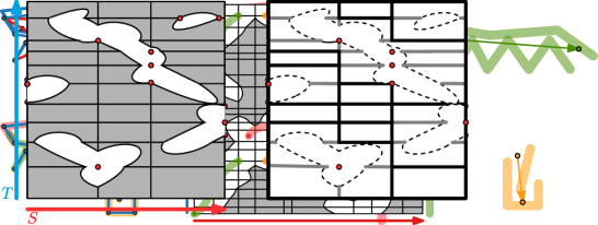
Figure 2: (top left) A simplification $S$ (red) of the trajectory $T$ (blue). (right) The free space diagram $\Delta^{\prime}\mathchar 45\relax\mathrm{FSD}(S,T)$. The clustering of $T$ corresponds to a set of colored bimonotone paths, where paths of a given color are horizontally aligned, and the paths together span the entire vertical axis.

For any $(\ell,\Delta)$-pathlet $(P,\mathcal{I})$ there exists an $(n,2\Delta)$-pathlet $(P^{\prime},\mathcal{I})$ where $P^{\prime}$ is a subcurve of $T$. Indeed, consider any interval $[a,b]\in\mathcal{I}$ and choose $P^{\prime}=T[a,b]$. However, restricting the subcurves of $T$ to have complexity at most $\ell$ may significantly reduce the maximum coverage, see for example Figure 3.

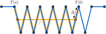
Figure 3: There exists a segment $P$ where $d_{F}(P,T[a,b])\leq\Delta$. In contrast, for any vertex-restricted $S$ with $d_{F}(T[a,b],S)\leq\Delta$, the complexity of $S$ is $\Theta(|T[a,b]|)$.

Instead of restricting pathlets to be subcurves of $T$, we will restrict them to be subcurves of a different curve $S$ which has the following properties:

Definition 5.1.

For a trajectory $T$ with $n$ vertices and $\Delta\geq 0$, a pathlet-preserving simplification is a curve $S$ together with a $2\Delta$-matching $(M^{ST},M^{TS})$ where:

1. For every edge $S[i,i+1]$ of $S$, we require that $S(i)=T(a)$, $S(i+1)=T(b)$ (for some $a,b\in[1,n]$) and that $d_{F}(T[a,b],S[i,i+1])\leq 2\Delta$.

2. For any subcurve $T[a,b]$ and all curves $P$ with $d_{F}(P,T[a,b])\leq\Delta$, the subcurve $S[s,t]$ (with $[s,t]=M^{TS}([a,b])$) has complexity $|S[s,t]|\leq|P|+2-|\mathbb{N}\cap\{s,t\}|$.

Theorem 5.2.

Let $(S,M^{ST},M^{TS})$ be a pathlet-preserving simplification of $T$. For any $(\ell,\Delta)$-pathlet $(P,\mathcal{I})$, there exists an $(\ell+2-|\mathbb{N}\cap\{s,t\}|,4\Delta)$-pathlet $(S[x,x^{\prime}],\mathcal{I})$.

Proof 5.3.

Consider any $(\ell,\Delta)$-pathlet $(P,\mathcal{I})$ and choose some interval $[y,y^{\prime}]\in\mathcal{I}$. For all $[a,b]\in\mathcal{I}$, via the triangle inequality, $d_{F}(T[y,y^{\prime}],T[a,b])\leq 2\Delta$. We apply Property (b) of a pathlet-preserving simplification $(S,M^{ST},M^{TS})$ to $T[y,y^{\prime}]$. This gives a curve $S[x,x^{\prime}]=M^{TS}(T[y,y^{\prime}])$ with $d_{F}(S[x,x^{\prime}],T[y,y^{\prime}])\leq 2\Delta$, and for which there exists no curve $P^{\prime}$ with $d_{F}(P^{\prime},T[y,y^{\prime}])\leq\Delta$ with $|P^{\prime}|<|S[x,x^{\prime}]|-2+|\mathbb{N}\cap\{a,b\}|$. In particular, setting $P^{\prime}\leftarrow P$ implies that $|S[x,x^{\prime}]|\leq\ell+2-|\mathbb{N}\cap\{a,b\}|$.

We may for every $[a,b]\in\mathcal{I}$ apply the triangle inequality once more to get that $d_{F}(S[x,x^{\prime}],T[a,b])\leq 4\Delta$. Thus $(S[x,x^{\prime}],\mathcal{I})$ is an $(\ell+2-|\mathbb{N}\cap\{a,b\}|,4\Delta)$-pathlet.

Prior curve simplifications.

The curve $S$ that we construct is a curve-restricted $\alpha\Delta$-simplification of $T$; a curve whose vertices lie on $T$, where for every edge $s=(T(a),T(b))$ of $S$ we have $d_{F}(s,T[a,b])\leq\alpha\Delta$. Various $\alpha\Delta$-simplifications and construction algorithms have been proposed before, see for example [18, 2, 15, 21].

If $T$ is a curve in $\mathbb{R}^{2}$, Guibas et al. [18] give an $\mathcal{O}(n\log n)$ time algorithm that for any $\alpha$ computes a $2\Delta$-simplification $S$ for which there is no $\Delta$-simplification $S^{\prime}$ with $|S^{\prime}|<|S|$. Their algorithm unfortunately is not efficient in higher dimensions, as it relies on maintaining the intersection of wedges to encode all line segments that simplify the currently scanned prefix curve. These wedges are formed by the tangents of a point to the various disks of radius $\Delta$ around the vertices of $T$. In higher dimensions, these wedges form cones, whose intersection is not of constant complexity.

Agarwal et al. [2] also construct a $2\Delta$-simplification $S$ of $T$ in $\mathcal{O}(n\log n)$ time. This was applied by Akitaya et al. [3] for their subtrajectory clustering algorithm under the discrete Fréchet distance. The simplification $S$ has a similar guarantee as the simplification of [18]: there exists no vertex-restricted $\Delta$-simplification $S^{\prime}$ with $|S^{\prime}|<|S|$. This simplification can be constructed efficiently in higher dimensions, but does not give guarantees with respect to arbitrary simplifications.

As we show in Figure 3, the complexity of a vertex-restricted $\Delta$-simplification can be arbitrarily bad compared to the (unrestricted) $\Delta$-simplification with minimum complexity. Brüning et al. [6] note that for the subtrajectory problem under the continuous Fréchet distance, one requires an $\alpha\Delta$-simplification whose complexity has guarantees with respect to the optimal unrestricted simplification. They present a $3\Delta$-simplification $S$ (whose definition was inspired by de Berg, Gudmundsson and Cook [15]) with the following property: for any subcurve $T[a,b]$ of $T$ within Fréchet distance $\Delta$ of some line segment, there exists a subcurve $S[s,t]$ of $T$ with complexity at most $4$ that has Fréchet distance at most $3\Delta$ to $T[a,b]$. This implies that there exists no $\Delta$-simplification $S^{\prime}$ with $|S^{\prime}|<|S|/2$.

Our new curve simplification.

In Definition 5.1 we presented yet another curve simplification under the Fréchet distance for curves in $\mathbb{R}^{d}$. Our simplification has two properties that we discuss here. Property (a) states that it is a $2\Delta$-simplification. Our Property (b) is a stronger version of the property that is realized by Brüning et al. [6]: for any subcurve $T[a,b]$ and any curve $P$ with $d_{F}(P,T[a,b])\leq\Delta$, we require that there exists a subcurve $S[s,t]$ with $d_{F}(S[s,t],T[a,b])\leq 2\Delta$ that has at most two more vertices than $P$. This implies both the property of Brüning et al. [6] and that there exists no $\Delta$-simplification $S^{\prime}$ with $|S^{\prime}|<|S|-2$.

We give an efficient algorithm for contructing pathlet-preserving simplifications in Section 10. The algorithm can be seen as an extension of the vertex-restricted simplification of Agarwal et al. [2] to construct a curve-restricted simplification instead. For this, we use the techniques of Guibas et al. [18] to quickly identify if an edge of $T$ is suitable to place a simplification vertex on. Then we combine this check with the algorithm of [2]. This results in the following:

Theorem 5.4.

For any trajectory $T$ and any $\Delta\geq 0$, we can construct a pathlet-preserving simplification $S$ in $\mathcal{O}(n\log n)$ time.

6 A greedy algorithm

6.1 Greedy set cover

Subtrajectory clustering is closely related to the set cover problem. In this problem, we have a discrete universe $\mathcal{U}$ and a family of sets $\mathcal{S}$ in this universe, and the goal is to pick a minimum number of sets in $\mathcal{S}$ such that their union is the whole universe. For subtrajectory clustering with target-discrete pathlets, we can set $\mathcal{U}=\{[i,i+1]\mid i\in[1,n-1]\cap\mathbb{N}\}$ and $\mathcal{S}=\{[i,i+1]\subseteq\bigcup\mathcal{I}\mid\text{there exists an $(\ell,\Delta)$-pathlet $(P,\mathcal{I})$}\}$. That is, the universe is the set of intervals parameterizing the edges of $T$, and $\mathcal{S}$ is the family of sets of edge parameterizations of $T$ that can be covered by a pathlet.

The decision variant of set cover is NP-complete [20]. However, the following greedy strategy gives an $\mathcal{O}(\log n)$ approximation of the minimal set cover size [13]. Suppose we have picked a set $\hat{\mathcal{S}}\subseteq\mathcal{S}$ that does not yet cover all of $\mathcal{U}$. The idea is then to add a set $S\in\mathcal{S}$ that maximizes $S\cap(\mathcal{U}\setminus\hat{\mathcal{S}})$, and repeat the procedure until $\mathcal{U}$ is fully covered.

We use this greedy strategy to focus on constructing a pathlet that covers the most uncovered edges of $T$. In other words, we greedily grow a set of pathlets $C$, each time adding a $(\ell,\Delta)$-pathlet $(P,\mathcal{I})$ that (approximately) maximizes the coverage $\lVert\mathrm{Cov}(P,\mathcal{I})\backslash\mathrm{Cov}(C)\rVert$. Our pathlets are target-discrete, in the sense that all endpoints of the intervals come from a discrete set of values.

We generalize the analysis of the greedy set cover argument to pathlets that cover a (constant) fraction of what the optimal pathlet covers. For this we introduce the following notion:

Definition 6.1 (Maximal pathlets).

Given a set $C$ of pathlets, a $(\Delta,\frac{1}{c})$-maximal $(\ell,\Delta^{\prime})$-pathlet $(P^{\prime},\mathcal{I}^{\prime})$ is a pathlet for which no $(\ell,\Delta)$-pathlet $(P,\mathcal{I})$ with

$$\frac{1}{c}\lVert\mathrm{Cov}(P,\mathcal{I})\setminus\mathrm{Cov}(C)\rVert\geq\lVert\mathrm{Cov}(P^{\prime},\mathcal{I}^{\prime})\setminus\mathrm{Cov}(C)\rVert.$$

In Lemma 6.2, we show that if we keep greedily selecting $(\Delta,\frac{1}{c})$-maximal pathlets for our clustering, the size of the clustering stays relatively small compared to the optimum size. The bound closely resembles the bound obtained by the argument for greedy set cover.

Lemma 6.2.

Let $T^{\prime}$ be a curve with $N$ vertices that is equal to $T$, up to reparameterization. Any algorithm that iteratively adds target-discrete $(\Delta,\frac{1}{c})$-maximal pathlets with respect to $T^{\prime}$ computes a (not necessarily target-discrete) clustering of $T$ of size at most $c\cdot k_{\ell}(\Delta)\ln N+1$.

Proof 6.3.

Let $C^{*}=\{(P_{i},\mathcal{I}_{i})\}_{i=1}^{k}$ be an $(\ell,\Delta)$-clustering of $T^{\prime}$ (and hence of $T$) of minimal size. Then $k\coloneqq|C^{*}|=k_{\ell}(\Delta)$. Consider iteration $j$ of the algorithm, where we have some set of $(\ell,\Delta^{\prime})$-clusters $C_{j}$. Denote by $W_{j}=\lVert[1,N]\setminus\mathrm{Cov}(C_{j})\rVert$ the remaining length that needs to be covered. Since $C^{*}$ covers $[1,N]$, it must cover $[1,N]\setminus\mathrm{Cov}(C_{j})$. It follows via the pigeonhole principle that there is at least one $(\ell,\Delta)$-pathlet $(P_{i},\mathcal{I}_{i})\in C^{*}$ for which the length $\lVert\mathrm{Cov}(P_{i},\mathcal{I}_{i})\setminus\mathrm{Cov}(C_{j})\rVert$ is at least $W_{j}/k$. Per definition of being $(\Delta,\frac{1}{c})$-maximal, our greedy algorithm finds a pathlet $(P_{j},\mathcal{I}_{j})$ that covers at least a $\frac{1}{c}$ fraction of the length that $(P_{i},\mathcal{I}_{i})$ covers. Thus:

$$W_{j+1}=\lVert[1,N]\setminus\left(\mathrm{Cov}(C_{j})\cup\mathrm{Cov}(P_{j},\mathcal{I}_{j})\right)\rVert\leq W_{j}-\frac{W_{j}}{c\cdot k}=W_{j}\cdot(1-\frac{1}{c\cdot k}).$$

Now we note that $W_{0}=N-1$. Suppose it takes $k^{\prime}+1$ iterations to cover all of $T^{\prime}$ with the greedy algorithm. Then before the last iteration, at least one edge of $T$ remained uncovered. That is, $(N-1)\cdot\left(1-\frac{1}{c\cdot k}\right)^{k^{\prime}}\geq 1$. From the inequality that $e^{x}\geq 1+x$ for all real $x$, we obtain that

$$\frac{1}{e}\geq\left(1-\frac{1}{x}\right)^{x}$$

for all $x\geq 1$. Plugging in $x\leftarrow c\cdot k$, it follows that

$$1\leq(N-1)\cdot\left(1-\frac{1}{c\cdot k}\right)^{k^{\prime}}=(N-1)\cdot\left(1-\frac{1}{c\cdot k}\right)^{c\cdot k\cdot\frac{k^{\prime}}{c\cdot k}}\leq(N-1)\cdot e^{-\frac{k^{\prime}}{c\cdot k}}.$$

Hence $e^{\frac{k^{\prime}}{c\cdot k}}\leq N$, showing that $k^{\prime}\leq c\cdot k\ln N$. Thus after $k^{\prime}+1\leq c\cdot k_{\ell}(\Delta)\ln N+1$ iterations, all of $T^{\prime}$ is covered.

6.2 Further restricting pathlets

Recall that with the pathlet-preserving simplification $S$ of $T$, we may restrict our attention to reference curves that are subcurves of $S$. Still, the space of possible reference curves is infinite. We wish to discretize this space by identifying certain finite classes of reference curves that contain a “good enough” reference curve, i.e., one with which we can construct a pathlet that is $(\Delta,\frac{1}{c})$-maximal for some small constant $c$.

We distinguish between four types of pathlets, based on their reference curves (note that not all pathlets fit into a class):

1. Vertex-to-vertex pathlets: A pathlet $(P,\mathcal{I})$ is a vertex-to-vertex pathlet if $P$ is a vertex-subcurve of $S$.

2. Prefix pathlets: A pathlet $(P,\mathcal{I})$ is a prefix pathlet if $P$ is the prefix of an edge of $S$.

3. Suffix pathlets: A pathlet $(P,\mathcal{I})$ is a suffix pathlet if $P$ is the suffix of an edge of $S$.

4. Subedge pathlets: A pathlet $(P,\mathcal{I})$ is a subedge pathlet if $P$ is a subcurve of an edge of $S$.

We construct pathlets of the above types that all cover at least some constant fraction of the optimal coverage for pathlets of the same type. Suppose we have a vertex-to-vertex $(\ell,\Delta^{\prime})$-pathlet $(P_{\mathrm{ver}},\mathcal{I}_{\mathrm{ver}})$ that covers at least a factor $\frac{1}{c_{\mathrm{ver}}}$ of what the optimal vertex-to-vertex $(\ell,\Delta)$-pathlet covers (with respect to the uncovered points). Additionally, suppose we have a prefix $(\ell,\Delta^{\prime})$-pathlet $(P_{\rm Phys.\leavevmode\nobreak\ Rev.\leavevmode\nobreak\ E},\mathcal{I}_{\rm Phys.\leavevmode\nobreak\ Rev.\leavevmode\nobreak\ E})$ that covers at least a factor $\frac{1}{c_{\rm Phys.\leavevmode\nobreak\ Rev.\leavevmode\nobreak\ E}}$ of what the optimal prefix $(\ell,\Delta)$-pathlet covers. Let $(P_{\mathrm{suf}},\mathcal{I}_{\mathrm{suf}})$ be a suffix $(\ell,\Delta^{\prime})$-pathlet that covers at least a factor $\frac{1}{c_{\mathrm{suf}}}$ of what the optimal suffix $(\ell,\Delta)$-pathlet covers. Finally, let $(P_{\mathrm{sub}},\mathcal{I}_{\mathrm{sub}})$ be a subedge $(\ell,\Delta^{\prime})$-pathlet that covers at least a factor $\frac{1}{c_{\mathrm{sub}}}$ of what the optimal subedge $(\ell,\Delta)$-pathlet covers. We show that the pathlet with maximum coverage out of the above three is $(\Delta,\frac{1}{c})$-maximal for $c=\max\{c_{\mathrm{ver}}+c_{\rm Phys.\leavevmode\nobreak\ Rev.\leavevmode\nobreak\ E}+c_{\mathrm{suf}},c_{\mathrm{sub}}\}$.

Lemma 6.4.

Given a collection $C$ of pathlets, let

$$(P,\mathcal{I})\in\{(P_{\mathrm{ver}},\mathcal{I}_{\mathrm{ver}}),(P_{\rm Phys.\leavevmode\nobreak\ Rev.\leavevmode\nobreak\ E},\mathcal{I}_{\rm Phys.\leavevmode\nobreak\ Rev.\leavevmode\nobreak\ E}),(P_{\mathrm{suf}},\mathcal{I}_{\mathrm{suf}}),(P_{\mathrm{sub}},\mathcal{I}_{\mathrm{sub}})\}$$

be the pathlet with maximal coverage among the uncovered points. Then $(P,\mathcal{I})$ is $(\Delta,\frac{1}{c})$-maximal with respect to $C$, for $c=\max\{c_{\mathrm{ver}}+c_{\rm Phys.\leavevmode\nobreak\ Rev.\leavevmode\nobreak\ E}+c_{\mathrm{suf}},c_{\mathrm{sub}}\}$.

Proof 6.5.

Let $(P^{*},\mathcal{I}^{*})$ be an optimal $(\ell,\Delta)$-pathlet. By Theorem 5.2, there exists a $\Delta^{\prime}$-pathlet $(S[x,x^{\prime}],\mathcal{I}^{*})$ with the same coverage, where $|S[x,x^{\prime}]|\leq\ell+2$ Suppose first that $S[x,x^{\prime}]$ is a subcurve of an edge of $S$, making $(S[x,x^{\prime}],\mathcal{I}^{*})$ a subedge pathlet with $|S[x,x^{\prime}]|\leq 2$. In this case, the coverage of $(P_{\mathrm{sub}},\mathcal{I}_{\mathrm{sub}})$ is at least $\frac{1}{c_{\mathrm{sub}}}$ times the coverage of $(S[x,x^{\prime}],\mathcal{I}^{*})$ over the uncovered points. Hence $(P_{\mathrm{sub}},\mathcal{I}_{\mathrm{sub}})$ is $(\Delta,\frac{1}{c_{\mathrm{sub}}})$-maximal. Since the pathlet $(P,\mathcal{I})$ has at least as much coverage as $(P_{\mathrm{sub}},\mathcal{I}_{\mathrm{sub}})$, it must also be $(\Delta,\frac{1}{c_{\mathrm{sub}}})$-maximal.

Next suppose that $S[x,x^{\prime}]$ is not the subcurve of an edge of $S$, meaning $S[x,x^{\prime}]$ contains at least one vertex of $S$. In this case, we split $S[x,x^{\prime}]$ into three subcurves:

• A suffix $P_{\mathrm{suf}}=S[x,\lceil x\rceil]$ of an edge,

• A vertex-subcurve $P_{\mathrm{ver}}=S[\lceil x\rceil,\lfloor x^{\prime}\rfloor]$, and

• A prefix $P_{\rm Phys.\leavevmode\nobreak\ Rev.\leavevmode\nobreak\ E}=S[\lfloor x^{\prime}\rfloor,x^{\prime}]$ of an edge.

Note that every subcurve has at most $\ell$ vertices, even if the suffix and/or prefix is empty (see Theorem 5.2).

Since every interval $[y,y^{\prime}]\in\mathcal{I}^{*}$ corresponds to a $\Delta^{\prime}$-matching $M$ between $S[x,x^{\prime}]$ and $T[y,y^{\prime}]$, we can decompose $[y,y^{\prime}]$ into three intervals $[y,y_{1}]$, $[y_{1},y_{2}]$ and $[y_{2},y^{\prime}]$, such that $M$ decomposes into three $\Delta^{\prime}$-matchings, one between $P_{\mathrm{suf}}$ and $T[y,y_{1}]$, one between $P_{\mathrm{ver}}$ and $T[y_{1},y_{2}]$, and one between $P_{\rm Phys.\leavevmode\nobreak\ Rev.\leavevmode\nobreak\ E}$ and $T[y_{2},y^{\prime}]$. By decomposing all intervals in $\mathcal{I}^{*}$ in this manner, we obtain that there are three $(\ell,\Delta)$-pathlets $(P_{\mathrm{suf}},\mathcal{I}^{*}_{\mathrm{suf}})$, $(P_{\mathrm{ver}},\mathcal{I}^{*}_{\mathrm{ver}})$ and $(P_{\rm Phys.\leavevmode\nobreak\ Rev.\leavevmode\nobreak\ E},\mathcal{I}^{*}_{\rm Phys.\leavevmode\nobreak\ Rev.\leavevmode\nobreak\ E})$ that together have the same coverage as $(P^{*},\mathcal{I}^{*})$.

We have at least one of the following:

• $(P_{\mathrm{suf}},\mathcal{I}^{*}_{\mathrm{suf}})$ covers at least a factor $\frac{c_{\mathrm{suf}}}{c_{\mathrm{ver}}+c_{\mathrm{suf}}+c_{\rm Phys.\leavevmode\nobreak\ Rev.\leavevmode\nobreak\ E}}$ of what $(P^{*},\mathcal{I}^{*})$ covers, or

• $(P_{\mathrm{ver}},\mathcal{I}^{*}_{\mathrm{ver}})$ covers at least a factor $\frac{c_{\mathrm{ver}}}{c_{\mathrm{ver}}+c_{\mathrm{suf}}+c_{\rm Phys.\leavevmode\nobreak\ Rev.\leavevmode\nobreak\ E}}$ of what $(P^{*},\mathcal{I}^{*})$ covers, or

• $(P_{\rm Phys.\leavevmode\nobreak\ Rev.\leavevmode\nobreak\ E},\mathcal{I}^{*}_{\rm Phys.\leavevmode\nobreak\ Rev.\leavevmode\nobreak\ E})$ covers at least a factor $\frac{c_{\rm Phys.\leavevmode\nobreak\ Rev.\leavevmode\nobreak\ E}}{c_{\mathrm{ver}}+c_{\mathrm{suf}}+c_{\rm Phys.\leavevmode\nobreak\ Rev.\leavevmode\nobreak\ E}}$ of what $(P^{*},\mathcal{I}^{*})$ covers.

Regardless of what statement holds, the pathlet $(P,\mathcal{I})$ covers at least a factor $\frac{1}{c_{\mathrm{ver}}+c_{\mathrm{suf}}+c_{\rm Phys.\leavevmode\nobreak\ Rev.\leavevmode\nobreak\ E}}$ of what $(P^{*},\mathcal{I}^{*})$ covers. Thus we have that $(P,\mathcal{I})$ is $(\Delta,\frac{1}{c_{1}+2c_{2}})$-maximal.

6.3 Subtrajectory clustering

We finish this section by combining the previous ideas on simplification and greedy algorithms to give our algorithm for subtrajectory clustering. The algorithm, given as pseudocode in Algorithm 1, uses subroutines for constructing the four types of pathlets given in Section 6.2.

Construct a pathlet-preserving simplification $(S,M^{ST},M^{TS})$ of $T$

Set $\Delta^{\prime}\leftarrow 4\Delta$

Set $C\leftarrow\emptyset$

while  $\mathrm{Cov}(C)\neq[1,n]$  do

       Construct a vertex-to-vertex $(\ell,\Delta^{\prime})$-pathlet $(P_{\mathrm{ver}},\mathcal{I}_{\mathrm{ver}})$ with the algorithm of Section 7

      Construct a prefix $(2,\Delta^{\prime})$-pathlet $(P_{\rm Phys.\leavevmode\nobreak\ Rev.\leavevmode\nobreak\ E},\mathcal{I}_{\rm Phys.\leavevmode\nobreak\ Rev.\leavevmode\nobreak\ E})$ with the algorithm of Section 8

      Construct a suffix $(2,\Delta^{\prime})$-pathlet $(P_{\mathrm{suf}},\mathcal{I}_{\mathrm{suf}})$ with the algorithm of Section 8

      Construct a subedge $(2,\Delta^{\prime})$-pathlet $(P_{\mathrm{sub}},\mathcal{I}_{\mathrm{sub}})$ with the algorithm of Section 9

      Set $(P,\mathcal{I})\in\{(P_{\mathrm{ver}},\mathcal{I}_{\mathrm{ver}}),(P_{\rm Phys.\leavevmode\nobreak\ Rev.\leavevmode\nobreak\ E},\mathcal{I}_{\rm Phys.\leavevmode\nobreak\ Rev.\leavevmode\nobreak\ E}),(P_{\mathrm{suf}},\mathcal{I}_{\mathrm{suf}}),(P_{\mathrm{sub}},\mathcal{I}_{\mathrm{sub}})\}$ to be the pathlet with maximum coverage over $[1,n]\setminus\mathrm{Cov}(C)$

      Add $(P,\mathcal{I})$ to $C$

return $C$

Algorithm 1 SubtrajectoryClustering($T$, $\ell$, $\Delta$)

6.3.1 A data structure for comparing pathlets

In each iteration of our greedy algorithm, we pick one of four pathlets whose coverage is the maximum over $[1,n]\setminus\mathrm{Cov}(C)$, given the current set of picked pathlets $C$. Computing the coverage of a pathlet $(P,\mathcal{I})$ can be done by first constructing $\bigcup\mathcal{I}$ and $\mathrm{Cov}(C)$, and then computing $\lVert I\setminus\mathrm{Cov}(C)\rVert$ for every component $I$ of $\bigcup\mathcal{I}$ seperately, adding up the results. In Lemma 6.6, we present a data structure for efficiently computing $\lVert I\setminus\mathrm{Cov}(C)\rVert$.

Lemma 6.6.

Let $m$ be the number of connected components of $\mathrm{Cov}(C)$. In $\mathcal{O}(m\log m)$ time, we can preprocess $\mathrm{Cov}(C)$ into a data structure of $\mathcal{O}(m)$ size, such that given an interval $I$, the value $\lVert I\setminus\mathrm{Cov}(C)\rVert$ can be computed in $\mathcal{O}(\log m)$ time.

Proof 6.7.

We store the connected components of $\mathrm{Cov}(C)$ in a binary search tree, ordering the intervals by increasing endpoints. Note that this ordering is well-defined, since the connected components are disjoint. We annotate each node of the tree with the total length of the intervals stored in it. The tree takes $\mathcal{O}(m\log m)$ time to construct and uses $\mathcal{O}(m)$ space.

To compute $\lVert I\setminus\mathrm{Cov}(C)\rVert$ for a given query interval $I$, we compute $\lVert I\cap\mathrm{Cov}(C)\rVert$ and subtract this value from the length of $I$. Because the components of $\mathrm{Cov}(C)$ are disjoint, there are at most two intervals that $I$ intersects but does not contain. These intervals can be reported in $\mathcal{O}(\log m)$ time with a range reporting query with the endpoints of $I$. In the same time bound, we can retrieve all intervals contained in $I$ as a set of $\mathcal{O}(\log m)$ nodes of the tree. By counting up the lengths these nodes are annotated with, we compute the total length of the intervals that are contained in $I$. Combined with the length of the overlap between the two intervals intersecting $I$ at its endpoints, we have computed $\lVert I\cap\mathrm{Cov}(C)\rVert$ in $\mathcal{O}(\log m)$ time.

The complexity of $\mathrm{Cov}(C)$ depends on how complex the pathlets in $C$ are. Specifically, if the endpoints of pathlets in $C$ come from a discrete set of $N$ values, then the number of connected components of $\mathrm{Cov}(C)$ is at most $\min\{\sum_{(P,\mathcal{I})\in C}|\mathcal{I}|,N\}$.

6.3.2 Constructing the pathlets

The algorithm, given as pseudocode in Algorithm 1, uses subroutines for constructing the four types of pathlets given in Section 6.2.

1. The first subroutine is for constructing a vertex-to-vertex $(\ell,\Delta^{\prime})$-pathlet whose coverage is at least half the coverage of an optimal vertex-to-vertex $(\ell,\Delta)$-pathlet, thus setting $c_{\mathrm{ver}}\leftarrow 2$.

2. The second subroutine is for constructing a prefix $(2,\Delta^{\prime})$-pathlet whose coverage is at least half the coverage of an optimal prefix $(2,\Delta)$-pathlet, thus setting $c_{\rm Phys.\leavevmode\nobreak\ Rev.\leavevmode\nobreak\ E}\leftarrow 2$. When restricted to target-discrete pathlets, we give an improved algorithm that returns an optimal pathlet, so $c_{\rm Phys.\leavevmode\nobreak\ Rev.\leavevmode\nobreak\ E}\leftarrow 1$ in this case.

3. The third subroutine is for constructing a suffix $(2,\Delta^{\prime})$-pathlet, which works symmetrically to that for prefix pathlets. Hence $c_{\mathrm{suf}}\leftarrow 2$, or $c_{\mathrm{suf}}\leftarrow 1$ in the target-discrete case.

4. The fourth and final subroutine is for constructing a subedge $(2,\Delta^{\prime})$-pathlet whose coverage is at least one-fourth the coverage of an optimal subedge $(2,\Delta)$-pathlet, thus setting $c_{\mathrm{sub}}\leftarrow 4$. When restricted to target-discrete pathlets, we give an improved algorithm that returns a pathlet with at least one-third the optimal coverage, so $c_{\rm Phys.\leavevmode\nobreak\ Rev.\leavevmode\nobreak\ E}\leftarrow 3$ in this case.

By Lemma 6.4, any pathlet $(P,\mathcal{I})$ added to the clustering in Algorithm 1 is $(\Delta,\frac{1}{c})$-maximal with respect to the at that point uncovered points, for $c=\max\{2+2+2,4\}=6$. By Lemma 6.2, the resulting $(\ell,\Delta^{\prime})$-clustering has size at most $6\cdot k_{\ell}(\Delta)\ln N+1$, where $N$ is the number of values that the intervals in a pathlet can use for their bounds. We show in our constructions of the pathlets that $N=\mathcal{O}(n^{4})$. In the target-discrete setting, we improve on this with $c=\max\{2+1+1,3\}=4$ and $N=n$, thus constructing a clustering of size at most $4\cdot k_{\ell}(\Delta)\ln n+1$.

Constructing the vertex-to-vertex pathlet takes $\mathcal{O}(n^{2}\log n\log\ell)$ time and uses $\mathcal{O}(n\ell\log n)$ space, in either setting (Theorem 7.13). The prefix and suffix pathlets take $\mathcal{O}(n^{3}\log^{2}n)$ time and $\mathcal{O}(n^{2}\log n)$ space to construct (Theorem 8.4). In the target-discrete setting, the running time is improved to $\mathcal{O}(n^{2}\log^{2}n)$ and the space to $\mathcal{O}(n\log n)$ (Theorem 8.1). The running times and space bounds for continuous and target-discrete subedge pathlets are the same as for prefix and suffix pathlets.

To decide which pathlet to use in the clustering, we use the data structure of Lemma 6.6. Let $C$ be the set of pathlets already chosen for the clustering, and let $m=\min\{\sum_{(P,\mathcal{I})\in C}|I|,N\}$. The data structure takes $\mathcal{O}(m\log m)$ time to construct and uses $\mathcal{O}(m)$ space. To compute the coverage of a pathlet $(P,\mathcal{I})$, we first construct $\bigcup\mathcal{I}$ in $\mathcal{O}(|\mathcal{I}|\log|\mathcal{I}|)$ time, and subsequently query the data structure $\mathcal{O}(|\mathcal{I}|)$ times, taking a total of $\mathcal{O}(|\mathcal{I}|\log m)$ time,

All our constructed pathlets $(P,\mathcal{I})$ have $|\mathcal{I}|\leq n$. As there are $\mathcal{O}(k_{\ell}(\Delta)\log n)$ iterations, we obtain that $m=\min\{\mathcal{O}(k_{\ell}(\Delta)\log n),N\}$. In the general setting, this makes $m=\mathcal{O}(n\cdot k_{\ell}(\Delta)\log n)=\mathcal{O}(n^{2}\log n)$. In the target-discrete setting, this improves to $m=\mathcal{O}(n)$. This results in the following main theorems:

Theorem 6.8.

Given a trajectory $T$ with $n$ vertices, as well as an integer $\ell\geq 2$ and value $\Delta\geq 0$, we can construct a target-discrete $(\ell,4\Delta)$-clustering of size at most $4k_{\ell}(\Delta)\ln n+1$ in $\mathcal{O}(k_{\ell}(\Delta)n^{2}\log^{3}n)$ time and using $\mathcal{O}(n\ell\log n)$ space.

Theorem 6.9.

Given a trajectory $T$ with $n$ vertices, as well as an integer $\ell\geq 2$ and value $\Delta\geq 0$, we can construct an $(\ell,4\Delta)$-clustering of size at most $24k_{\ell}(\Delta)\ln\mathcal{O}(n)+1$ in $\mathcal{O}(k_{\ell}(\Delta)n^{3}\log^{3}n)$ time and using $\mathcal{O}(n^{2}\log n)$ space.

7 Vertex-to-vertex pathlets

In this section we give algorithms for constructing vertex-to-vertex pathlets that cover at least half of what the optimal vertex-to-vertex pathlet covers. Our algorithms rely on a data structure for computing reachability information in the free space, which we present in Section 7.1. In Section 7.2, we then construct an optimal pathlet $(P,\mathcal{I})$, where the reference curve $P$ is a given subcurve of $S$. In Section 7.4, we then apply this algorithm to $\mathcal{O}(n\log\ell)$ vertex-subcurves of $S$ to obtain a vertex-to-vertex pathlet of the desired quality.

7.1 A data structure for constructing optimal pathlets

Let $W$ be a curve with $\mathcal{O}(\ell)$ vertices, of which $P$ is a subcurve. We construct a reachability graph $G(W,T)$ of complexity $\mathcal{O}(n\ell\log n)$ that encodes reachability between certain points in the free space. For our purposes, it is sufficient to consider the following critical points.

Definition 7.1.

Any side of any grid cell intersects $\Delta^{\prime}\mathchar 45\relax\mathrm{FSD}(W,T)$ in a vertical or horizontal segment [5]. The critical points $R$ of $\Delta^{\prime}\mathchar 45\relax\mathrm{FSD}(W,T)$ are the endpoints of these segments. All points $(i,j)\in\Delta^{\prime}\mathchar 45\relax\mathrm{FSD}(W,T)$ with integer coordinates are critical points.

Let $Z$ be the set of critical points of $\Delta^{\prime}\mathchar 45\relax\mathrm{FSD}(W,T)$. We store a data structure over $G(W,T)$ that may be queried with two points $(x,y)$ and $(x^{\prime},y^{\prime})$ from $Z$, and returns in $\mathcal{O}(\log n)$ time whether $(x^{\prime},y^{\prime})$ is reachable from $(x,y)$ in $G(W,T)$. Recall that this implies that $d_{F}(W[x,x^{\prime}],T[y,y^{\prime}])\leq\Delta^{\prime}$. Furthermore, our data structure can retrieve for any point $(x^{\prime},y^{\prime})\in Z$ the minimum value $x$ for which there exists a value $y$ with $d_{F}(W[x,x^{\prime}],T[y,y^{\prime}])\leq\Delta^{\prime}$ in constant time. These queries play an important role in our algorithms for computing pathlets (see Sections 7.2 and 7.3).

Constructing the graph $G(W,T)$.

We compute $Z$ in $\mathcal{O}(n\ell)$ time through the classical algorithm to compute $d_{F}(W,T)$ [4], which constructs the free space diagram. In Lemma 7.2 we observe that when focusing on reachability between points in $\Delta^{\prime}\mathchar 45\relax\mathrm{FSD}(W,T)$, we can simplify $\Delta^{\prime}\mathchar 45\relax\mathrm{FSD}(W,T)$ by replacing each obstacle of $\Delta^{\prime}\mathchar 45\relax\mathrm{FSD}(W,T)$ by a rectilinear polygon. Specifically, for an integer-coordinate point $(i,j)$ that is not in free space, let $I_{h}(i,j)=[x,x^{\prime}]\times\{j\}$ and $I_{v}(i,j)=\{i\}\times[y,y^{\prime}]$ be the maximum horizontal and vertical segments containing $(i,j)$ that are interior-disjoint from $\Delta^{\prime}\mathchar 45\relax\mathrm{FSD}(W,T)$. We model the obstacles in $\Delta^{\prime}\mathchar 45\relax\mathrm{FSD}(W,T)$ as the union of these segments: $\bigcup_{(i,j)}(I_{h}(i,j)\cup I_{v}(i,j))$. The area $[1,\ell]\times[1,n]$ minus all these rectilinear obstacles gives a rectilinear polygon with rectilinear holes $\mathcal{R}$. See Figure 4 for an illustration.

Figure 4: (left) The $\Delta^{\prime}$-free space diagram of $W$ and $T$ with the critical points. (right) The rectilinear obstacles $\mathcal{R}$ consist of are all grid edges that are entirely contained in the obstacles of $\Delta^{\prime}\mathchar 45\relax\mathrm{FSD}(W,T)$ (shown in black) plus the gray segments.

Lemma 7.2.

Let $p$ and $q$ be two points in $\Delta^{\prime}\mathchar 45\relax\mathrm{FSD}(W,T)$. There is a bimonotone path from $p$ to $q$ in $\Delta^{\prime}\mathchar 45\relax\mathrm{FSD}(W,T)$ if and only if there is a bimonotone path from $p$ to $q$ in $\mathcal{R}$.

Proof 7.3.

Since $\Delta^{\prime}\mathchar 45\relax\mathrm{FSD}(W,T)$ is completely contained in $\mathcal{R}$, we immediately have that a bimonotone path from $p$ to $q$ in $\Delta^{\prime}\mathchar 45\relax\mathrm{FSD}(W,T)$ is also a bimonotone path in $\mathcal{R}$. Next consider a bimonotone path $\pi$ from $p$ to $q$ in $\mathcal{R}$. This path goes through a sequence of cells $c_{1},\dots,c_{k}$ of the free space diagram (but in $\mathcal{R}$). The intersection points between $\pi$ and these cells all lie in $\Delta^{\prime}\mathchar 45\relax\mathrm{FSD}(W,T)$, by construction of $\mathcal{R}$. By convexity of the free space inside cells, we may connect the sequence of intersection points by interpolating line segments to obtain a bimonotone path from $p$ to $q$ in $\Delta^{\prime}\mathchar 45\relax\mathrm{FSD}(W,T)$.

To obtain a reachability graph $G(W,T)$ we construct an undirected graph $G(Z)$. This graph is the shortest paths preserving graph by Widmayer [22], defined over the set of points $Z$ that we are interested in. This graph is defined as follows. Let $x_{1},\dots,x_{m}$ be the increasing sequence of distinct $x$-coordinates of points in $Z$. We distinguish two cases.

• If $m=1$, then all points lie on the vertical line $x=x_{m}$. The graph $G(Z)$ is the path graph connecting points in $Z$ that are adjacent on this line.

• If $m>1$, consider a value $\bar{x}$ with $x_{\lfloor m/2\rfloor}<\bar{x}<x_{\lfloor m/2\rfloor+1}$. Partition $Z$ into the sets $Z_{\text{left}}=\{(x,y)\in Z\mid x<\bar{x}\}$ and $Z_{\text{right}}=\{(x,y)\in Z\mid x>\bar{x}\}$. Let $G(Z_{\text{left}})$ and $G(Z_{\text{right}})$ be their shortest paths preserving graphs. We combine $G(Z_{\text{left}})$ and $G(Z_{\text{right}})$ into $G(Z)$ by adding Steiner points on the line $x=\bar{x}$. For every $p=(x,y)\in Z$, if the horizontal segment $\overline{pq}$ with $q=(\bar{x},y)$ lies fully in $\mathcal{R}$, we add $q$ as a Steiner point and add edge $(p,q)$ to the graph. Also, we connect adjacent Steiner points on the line $x=\bar{x}$ by an edge.

The graph $G(Z)$ has size $\mathcal{O}(n\ell\log n\ell)=\mathcal{O}(n\ell\log n)$ and can be constructed in $\mathcal{O}(n\ell\log n)$ time [22]. By assigning each edge $e\in E$ a weight equal to its length, the graph perfectly encodes rectilinear distances between points in $Z$. That is, the rectilinear distance in $\mathcal{R}$ between two points in $Z$ is equal to their distance in $G(Z)$.

The edges of $G(Z)$ all horizontal or vertical line segments. We set $G(W,T)$ to be the graph $G(Z)$, but with each edge directed towards the right (if horizontal) or top (if vertical). Next, observe that $G(W,T)$ perfectly encodes reachability: for two points $p=(x,y)$ and $q=(x^{\prime},y^{\prime})$ in $Z$, if there is a bimonotone rectilinear path from $p$ to $q$ in $\mathcal{R}$, then any rectilinear shortest path from $p$ to $q$ must be bimonotone, and hence there must be a bimonotone path between them in $G(W,T)$. Conversely, any path in $G(W,T)$ is also a path in $\mathcal{R}$. Thus $d_{F}(P[x,x^{\prime}],T[y,y^{\prime}])\leq\Delta^{\prime}$ if and only if there is a (bimonotone) path from $(x,y)$ to $(x^{\prime},y^{\prime})$ in $G(W,T)$.

The graph $G(W,T)$ is a directed planar graph. We use the following data structure to handle reachability queries in $G(W,T)$ in just logarithmic time. Preprocessing time and space are $\mathcal{O}(n\ell\log n)$, linear in the size of $G(W,T)$.

Lemma 7.4 (Holm et al. [19]).

Any planar directed graph with $n$ vertices can be preprocessed in $\mathcal{O}(n)$ time and space to answer reachability queries in $\mathcal{O}(\log n)$ time.

Corollary 7.5.

In $\mathcal{O}(n\ell\log n)$ time, we can preprocess $W$ and $T$ into a data structure of $\mathcal{O}(n\ell\log n)$ size, such that for any two critical points $(x,y)$ and $(x^{\prime},y^{\prime})$, we can determine if $d_{F}(W[x,x^{\prime}],T[y,y^{\prime}])\leq\Delta^{\prime}$ in $\mathcal{O}(\log n)$ time.

Next we annotate $G(W,T)$ to support the second type of queries. Recall that this second type asks, for a given critical point $(x^{\prime},y^{\prime})$, what the minimum value $x$ is for which there exists a value $y$ with $d_{F}(W[x,x^{\prime}],T[y,y^{\prime}])\leq\Delta^{\prime}$. We simply annotate each vertex $(x^{\prime},y^{\prime})$ of $G(W,T)$ with its corresponding minimum $x$. Since the critical points $(x,y)$ with $d_{F}(W[x,x^{\prime}],T[y,y^{\prime}])\leq\Delta^{\prime}$ are precisely those that can reach $(x^{\prime},y^{\prime})$ in $G(W,T)$, this information can be computed in $\mathcal{O}(n\ell\log n)$ time by applying depth-first search on $G(W,T)$. Thus, we conclude:

Theorem 7.6.

Let $W$ be a curve with $\ell$ vertices. In $\mathcal{O}(n\ell\log n)$ time, we can preprocess $W$ and $T$ into a data structure of $\mathcal{O}(n\ell\log n)$ size that answers the following queries:

1. Given two critical points $(x,y)$ and $(x^{\prime},y^{\prime})$, we can report if $d_{F}(W[x,x^{\prime}],T[y,y^{\prime}])\leq\Delta^{\prime}$ in $\mathcal{O}(\log n)$ time.

2. Given a critical point $(x^{\prime},y^{\prime})$, we can report the minimum value $x$ for which there exists a value $y$ with $d_{F}(W[x,x^{\prime}],T[y,y^{\prime}])\leq\Delta^{\prime}$ in $\mathcal{O}(1)$ time.

7.2 Constructing a vertex-to-vertex pathlet for a given reference curve

In this section we present an algorithm for constructing vertex-to-vertex pathlets when the reference curve $P$ (with at most $\ell$ vertices) is given. We assume that we have the reachability graph data structure $G(W,T)$ of Theorem 7.6 built for some curve $W$ of which $P$ is a subcurve. Given a set of pathlets $C$, our algorithm reports an $(\ell,\Delta^{\prime})$-pathlet $(P,\mathcal{I})$ maximizing $\lVert\mathrm{Cov}(P,\mathcal{I})\setminus\mathrm{Cov}(C)\rVert$ in $\mathcal{O}(n\log n)$ time.

We construct the optimal pathlet $(P,\mathcal{I})$ as follows: For every integer $j^{\prime}\in[1,n]$, we consider the maximal interval $[j,j^{\prime}]$ for which $d_{F}(P,T[j,j^{\prime}])\leq\Delta^{\prime}$, and if it exists, we add it to $\mathcal{I}$. This trivially maximizes $\mathrm{Cov}(P,\mathcal{I})\setminus\mathrm{Cov}(C)$. In the following lemma, we show that we can compute these maximal intervals in $\mathcal{O}(n\log n)$ time in total, given the reachability graph.

Lemma 7.7.

Given the reachability graph data structure $G(W,T)$ of Theorem 7.6, we can compute, for all integers $j^{\prime}\in[1,n]$, the maximal interval $[j,j^{\prime}]$ for which $d_{F}(P,T[j,j^{\prime}])\leq\Delta^{\prime}$ in $\mathcal{O}(n\log n)$ time altogether.

Proof 7.8.

Let $P=W[i,i^{\prime}]$ and denote by $J^{\prime}$ the subset of integers $j^{\prime}\in[1,n]$ for which there exists an integer $j$ with $d_{F}(P=W[i,i^{\prime}],T[j,j^{\prime}])\leq\Delta^{\prime}$. Observe that the set $J^{\prime}$ consists of precisely those integers $j^{\prime}$ for which query (b) from Theorem 7.6 for the point $(i^{\prime},j^{\prime})$ reports a value $x\leq i$. Thus, we may compute $J^{\prime}$ in $\mathcal{O}(n)$ total time by iterating over all integers in $[1,n]$. We then immediately report the empty interval for all $j^{\prime}\notin J^{\prime}$.

For each $j^{\prime}\in J^{\prime}$ we compute the minimum integer $j$ for which $d_{F}(P,T[j,j^{\prime}])\leq\Delta^{\prime}$. This integer corresponds to the lowest point $(i,j)$ on the left side of $\Delta^{\prime}\mathchar 45\relax\mathrm{FSD}(P,T)$ that can reach $(i^{\prime},j^{\prime})$ by a bimonotone path. By planarity, no point $(i,\hat{j})$ with $\hat{j}<j$ can reach $(i^{\prime},\hat{j}^{\prime})$ when $\hat{j}^{\prime}\geq j^{\prime}$. We use this fact to scan over the integers in $J^{\prime}$ in ascending order and conservatively scan over the integer-coordinate points on the left side. For each considered pair of integers $j\in[1,n]$ and $j^{\prime}\in J^{\prime}$, we query the reachability graph to check whether $(i,j)$ can reach $(i^{\prime},j^{\prime})$. If the query returns positive, $[j,j^{\prime}]$ is the maximal interval for integer $j^{\prime}$ for which $d_{F}(P,T[j,j^{\prime}])\leq\Delta^{\prime}$. We report $[j,j^{\prime}]$ and set $j^{\prime}$ to the next value in $J^{\prime}$. If the query returns negative, $d_{F}(P,T[\hat{j},j^{\prime}])>\Delta^{\prime}$ for all $\hat{j}\leq j$, so we search among higher values for $j$. The query takes $\mathcal{O}(\log n)$ time, and we make $\mathcal{O}(n)$ queries, giving the claimed running time.

Lemma 7.9.

Let $C$ be a set of pathlets, $W$ be a curve and let $P$ be a vertex-subcurve of $W$ with at most $\ell$ vertices. Given the reachability graph data structure $G(W,T)$ of Theorem 7.6, we can construct a target-discrete $(\ell,\Delta^{\prime})$-pathlet $(P,\mathcal{I})$ that maximizing $\lVert\mathrm{Cov}(P,\mathcal{I})\setminus\mathrm{Cov}(C)\rVert$ in $\mathcal{O}(n\log n)$ time.

7.3 Constructing a fully continuous pathlet for a given reference curve

Next we lift the target-discrete restriction on the pathlets. To do so, we add $\mathcal{O}(n)$ breakpoints to $T$ that allow us to restrict pathlets to be target-discrete without sacrificing quality. For every critical point of the form $(i,y)$ (resp. $(i^{\prime},y^{\prime})$), i.e., those on the left (resp. right) sides of $\Delta^{\prime}\mathchar 45\relax\mathrm{FSD}(P,T)$, we add a breakpoint at $T(y)$ (resp. $T(y^{\prime})$). Let $T^{\prime}$ be the curve where breakpoints are seen as vertices, so they are indexed by integers. Let $n^{\prime}=\mathcal{O}(n)$ be the number of vertices of $T^{\prime}$. In Lemma 7.10 we show that the breakpoints allow us to restrict pathlets to be target-discrete on $T^{\prime}$.

Lemma 7.10.

For any vertex-to-vertex $(\ell,\Delta^{\prime})$-pathlet $(P,\mathcal{I})$, there exists a target-discrete vertex-to-vertex $(\ell,\Delta^{\prime})$-pathlet $(P,\mathcal{I}^{\prime})$ with $\mathrm{Cov}(P,\mathcal{I}^{\prime})\supseteq\mathrm{Cov}(P,\mathcal{I})$.

Proof 7.11.

Let $I=[y,y^{\prime}]$ be an interval in $\mathcal{I}$. Because $(P,\mathcal{I})$ is an $(\ell,\Delta^{\prime})$-pathlet, there exists a bimonotone path from $(i,y)$ to $(i^{\prime},y^{\prime})$ in $\Delta^{\prime}\mathchar 45\relax\mathrm{FSD}(S,T^{\prime})$. By our definition of the breakpoints, the vertical segments $\{i\}\times[\lfloor y\rfloor,\lceil y\rceil]$ and $\{i^{\prime}\}\times[\lfloor y^{\prime}\rfloor,\lceil y^{\prime}\rceil]$ lie in free space. Hence $(i,\lfloor y\rfloor)$ can reach $(i^{\prime},\lceil y^{\prime}\rceil)$ by a bimonotone path. We replace $I$ by $[\lfloor y\rfloor,\lceil y^{\prime}\rceil]$ and let $\mathcal{I}^{\prime}$ be the set of intervals obtained by replacing all intervals in $\mathcal{I}$ in this manner. The pathlet $(P,\mathcal{I}^{\prime})$ is a target-discrete $(\ell,\Delta^{\prime})$-pathlet with $\mathrm{Cov}(P,\mathcal{I}^{\prime})\supseteq(P,\mathcal{I})$.

Observe that while the reachability graph $G(P,T^{\prime})$ is different from $G(P,T)$, the critical points on the left and right sides of the free space diagram are present in both graphs (although with different coordinates due to the reparameterization). Thus we may still use $G(P,T)$ for reachability information between these points, and we can therefore use $G(P,T)$ to compute, for all integers $j^{\prime}\in[1,n^{\prime}]$, the maximal interval $[j,j^{\prime}]$ for which $d_{F}(P,T[j,j^{\prime}])\leq\Delta^{\prime}$ in $\mathcal{O}(n^{\prime}\log n^{\prime})=\mathcal{O}(n\log n)$ time. Since this interval uses only $y$-coordinates of critical values on the left and right sides of $\Delta^{\prime}\mathchar 45\relax\mathrm{FSD}(P,T)$ for its endpoints, we obtain that the endpoints come from a set of $\mathcal{O}(n)$ values. We hence obtain:

Lemma 7.12.

Let $C$ be a set of pathlets and $P$ be a vertex-subcurve of $S$. Given the reachability graph $G(P,T)$ of Theorem 7.6, we can construct in $\mathcal{O}(n\log n)$ time an $(\ell,\Delta^{\prime})$-pathlet $(P,\mathcal{I})$ maximizing $\lVert\mathrm{Cov}(P,\mathcal{I})\setminus\mathrm{Cov}(C)\rVert$. The intervals in $\mathcal{I}$ all have endpoints that come from a set of $\mathcal{O}(n)$ values.

7.4 Constructing a good vertex-to-vertex pathlet

We finish this section with the following theorem regarding constructing good vertex-to-vertex pathlets:

Theorem 7.13.

Let $C$ be a set of pathlets. In $\mathcal{O}(n^{2}\log n\log\ell)$ time and using $\mathcal{O}(n\ell\log n)$ space, we can construct a (target-discrete) $(\ell,\Delta^{\prime})$-pathlet $(P,\mathcal{I})$ with

$$\lVert\mathrm{Cov}(P,\mathcal{I})\setminus\mathrm{Cov}(C)\rVert\geq\frac{1}{2}\lVert\mathrm{Cov}(P^{\prime},\mathcal{I}^{\prime})\setminus\mathrm{Cov}(C)\rVert$$

for any (target-discrete) vertex-to-vertex $(\ell,\Delta^{\prime})$-pathlet $(P^{\prime},\mathcal{I}^{\prime})$.

Proof 7.14.

We can construct the reachability graph data structure $G(W,T)$ for $W\leftarrow S$ and subsequently apply Lemmas 7.9 and 7.12 to all $\Theta(n\ell)$ vertex-subcurves of $T$ with complexity at most $\ell$. Both algorithms (for constructing either a target-discrete or a fully continuous pathlet given a reference curve) take $\mathcal{O}(n\log n)$ time given $G(W,T)$. This gives a running time of $\mathcal{O}(n^{2}\ell\log n)$ and a space usage of $\mathcal{O}(n^{2})$. To achieve the stated bounds, we use two optimizations.

First we observe that by sacrificing the quality of the pathlet slightly, and settling for a pathlet with at least half the coverage of the optimal pathlet, we can reduce the number of reference curves we have to consider from $\Theta(n\ell)$ to $\Theta(n\log\ell)$.

Let $(S[i,i^{\prime}],\mathcal{I})$ be a vertex-to-vertex pathlet. We can split $S[i,i^{\prime}]$ into two vertex-subcurves $S[i,i+2^{j}]$ and $S[i^{\prime}-2^{j},i^{\prime}]$ that each have a number of edges equal to a power of two. The matchings corresponding to $\mathcal{I}$ naturally decompose into two sets of matchings, giving rise to two pathlets $(S[i,i+2^{j}],\mathcal{I}_{1})$ and $(S[i^{\prime}-2^{j},i^{\prime}],\mathcal{I}_{2})$ with $\mathcal{I}_{1}\cup\mathcal{I}_{2}=\mathcal{I}$. Thus at least one of these pathlets has at least half the coverage that $(S[i,i^{\prime}],\mathcal{I})$ has.

We now limit our attention to reference curves that have a number of edges equal to a power of two. For vertex-subcurves with at most $\ell$ vertices, there are $\Theta(n\log\ell)$ such curves. This improves the total running time to $\mathcal{O}(n^{2}\log n\log\ell)$.

Next we observe that we do not need to have the entire graph $G(S,T)$ in memory, but only large enough parts of it that contain the reference curves we want to construct pathlets for. To make use of this observation, we assume for ease of exposition that $|S|=m\cdot\ell+1$ and we consider the set $\mathcal{W}_{S}=\{S[i,i+2\ell]\mid i=j\ell+1$, $j\in\{0,\dots,|S|-2\}\}$. This set contains $\mathcal{O}(|S|/\ell)=\mathcal{O}(n/\ell)$ vertex-subcurves of $S$, each with $2\ell$ vertices. Note that each vertex-subcurve $P$ of $S$ with at most $\ell$ vertices is a subcurve of some curve in $\mathcal{W}_{S}$. We iteratively go over the curves $W\in\mathcal{W}_{S}$, constructing $G(W,T)$ and then constructing pathlets for all reference curves that are subcurves of $W$ (and that have a number of edges equal to a power of two). The size of $G(W,T)$ is $\mathcal{O}(n\ell\log n)$, and constructing the graph for all curves in $\mathcal{W}_{S}$ takes a total of $\mathcal{O}((n/\ell)\cdot n\ell\log n)=\mathcal{O}(n^{2}\log n)$ time.

8 Prefix and suffix pathlets

8.1 Target-discrete pathlets

In this section we present an algorithm that constructs a target-discrete $(2,\Delta^{\prime})$-pathlet $(P,\mathcal{I})$ where $P$ is restricted to be a prefix $e[1,x^{\prime}]$ of some directed line segment $e$. We are given a collection $C$ of $(\ell,\Delta^{\prime})$-pathlets, and return a target-discrete pathlet that maximizes $\lVert\mathrm{Cov}(P,\mathcal{I})\setminus\mathrm{Cov}(C)\rVert$ in $\mathcal{O}(n\log n)$ time and $\mathcal{O}(n)$ space. Our algorithm can be applied to the symmetric situation where $P$ is restricted to be a suffix $e[x,2]$ of $e$.

For a fixed $x^{\prime}\in[1,2]$ there is an optimal target-discrete pathlet $(e[1,x^{\prime}],\mathcal{I})$ where $\mathcal{I}$ contains all maximum intervals $[j,j^{\prime}]$ with integer bounds for which $d_{F}(e[1,x^{\prime}],T[j,j^{\prime}])\leq\Delta^{\prime}$. Note that these intervals are independent of $C$. We use this observation to construct optimal prefix pathlets $(e[1,x^{\prime}],\mathcal{I})$ for all $x^{\prime}$, and additionally take into account the collection $C$ when choosing the right value for $x^{\prime}$.

We give a sweepline algorithm that sweeps over $\Delta^{\prime}\mathchar 45\relax\mathrm{FSD}(e,T)$ with a vertical line from left to right. During the sweep, we maintain the set of maximum intervals $\mathcal{I}(x^{\prime})$ for the current value of $x^{\prime}$. We make use of the reachability graph $G(e,T)$ of Theorem 7.6, which uses $\mathcal{O}(n\log n)$ space and can be constructed in $\mathcal{O}(n\log n)$ time. Additionally, we use the following observation regarding when the sets change.

Let $(x_{1},y_{1}),\dots,(x_{m},y_{m})$ be the $\mathcal{O}(n)$ endpoints of the horizontal segments formed by the intersections between grid cells and the free space, with $x_{1}\leq\dots\leq x_{m}$. Then for all integers $i$ and $x_{i}<x^{\prime}_{1}\leq x^{\prime}_{2}<x_{i+1}$, $\mathcal{I}(x^{\prime}_{1})=\mathcal{I}(x^{\prime}_{2})$.

Consider sweeping over $\Delta^{\prime}\mathchar 45\relax\mathrm{FSD}(e,T)$ with a vertical line from left to right. Let $(x_{1},y_{1}),\dots,(x_{m},y_{m})$ be the $\mathcal{O}(n)$ endpoints of the horizontal segments formed by the intersections between grid cells and the free space, where we assume for ease of exposition that $x_{1}<\dots<x_{m}$, so the $x$-coordinates are unique. When the sweepline reaches the left endpoint $(x_{i},y_{i})$ of a horizontal segment, a vertical passage opens up and points $(1,j)$ with $j\leq y_{i}$ may now reach $(x_{i},y_{i})$ and higher points. Let $(x_{i},j^{\prime})$ be the highest point with $j^{\prime}$ an integer for which $\{x_{i}\}\times[y_{i},j^{\prime}]\subseteq\Delta^{\prime}\mathchar 45\relax\mathrm{FSD}(e,T)$. We compute the minimum integer $j$ for which $(1,j)$ can reach $(x_{i},j^{\prime})$, and add $[j,j^{\prime}]$ to $\mathcal{I}(x_{i})$. Observe that if $(1,j)$ can reach $(x_{i},j^{\prime})$ for some integer $j$, then all points $(1,\hat{j})\in\Delta^{\prime}\mathchar 45\relax\mathrm{FSD}(e,T)$ with $j\leq\hat{j}\leq j^{\prime}$ can reach $(x_{i},j^{\prime})$. Thus we have a sort-of monotonicity and we can apply binary search over the points on the left side of the free space diagram that are in free space. To check for reachability, we make use of the reachabily graph $G(e,T)$. Every step of the binary search we query $G(e,T)$, taking $\mathcal{O}(\log n)$ time per step, totalling $\mathcal{O}(\log^{2}n)$ time to compute $j$.

When the sweepline reaches the right endpoint $(x_{i},y_{i})$ of a horizontal segment, the point $(x_{i},y_{i})$ becomes unreachable. However, all other points on the sweepline remain reachable from the same points on the left side. Thus we merely have to remove the interval $[j,y_{i}]$ that ends in $y_{i}$, if it is present in the current set of intervals. This takes only constant time.

In either of the above events, we create or remove a single interval. To keep track of the coverage of $\mathcal{I}(x^{\prime})$ with respect to $[1,n]\setminus\mathrm{Cov}(C)$ as we make these updates, we recall the data structure of Lemma 6.6:

See 6.6

We may assume that for any two pathlets $(P,\mathcal{I})$ and $(P^{\prime},\mathcal{I}^{\prime})$ in $C$, there are no two intervals $I\in\mathcal{I}$ and $I^{\prime}\in\mathcal{I}^{\prime}$ with $I\subseteq I^{\prime}$, as otherwise, $I$ would not contribute anything to the coverage and can therefore be ignored. This means that $\sum_{(P,\mathcal{I})\in C}|\mathcal{I}|<n$.

After $\mathcal{O}(n\log n)$ time preprocessing for the reachability graph $G(e,T)$ and the above data structure, we perform $\mathcal{O}(n)$ updates during the sweep, each taking $\mathcal{O}(\log^{2}n)$ time. As we maintain the coverage of the current set of intervals among the uncovered points, we know what prefix of $e$ gives the best pathlet after the sweep. This gives a construction time of $\mathcal{O}(n\log^{2}n)$ for a target-discrete prefix pathlet, given the edge $e$. Applying this algorithm to all edges of $S$ gives the following result.

Theorem 8.1.

Let $C$ be a set of pathlets and $\Delta^{\prime}\geq 0$. In $\mathcal{O}(n^{2}\log^{2}n)$ time and using $\mathcal{O}(n\log n)$ space, we can construct a target-discrete prefix $(2,\Delta^{\prime})$-pathlet $(P,\mathcal{I})$ maximizing $\lVert\mathrm{Cov}(P,\mathcal{I})\setminus\mathrm{Cov}(C)\rVert$.

8.2 Fully continuous pathlets

Next we lift the target-discrete restriction on the pathlets. We again focus on prefix pathlets; symmetric results hold for suffix pathlets. Like for continuous vertex-to-vertex pathlets, we add breakpoints to $T$ that allow us to restrict pathlets to be target-discrete. Let $(x_{i},y_{i})$ be the highest point of $\Delta^{\prime}\mathchar 45\relax\mathrm{FSD}(e,T)\cap[i,i+1]$, picking the leftmost highest point if multiple exist. For $i=1,\dots,n-1$, we add breakpoints at $T(y)$ for every highest point $(x_{i},y)$ of a connected component of $(\{x_{i}\}\times[1,n])\cap\Delta^{\prime}\mathchar 45\relax\mathrm{FSD}(e,T)$. Let $T^{\prime}$ be the curve where breakpoints are seen as vertices, so they are indexed by integers. Let $n^{\prime}=\mathcal{O}(n^{2})$ be the number of vertices of $T^{\prime}$. In Lemma 8.2 we show that the breakpoints allow us to restrict pathlets to be target-discrete on $T^{\prime}$, if we sacrifice coverage slightly.

Lemma 8.2.

Let $C$ be a set of pathlets. For any prefix $(2,\Delta^{\prime})$-pathlet $(e[1,x^{\prime}],\mathcal{I})$, there exists a target-discrete $(2,\Delta^{\prime})$-pathlet $(e[1,x^{\prime\prime}],\mathcal{I}^{\prime})$ with

$$\lVert\mathrm{Cov}(e[1,x^{\prime\prime}],\mathcal{I}^{\prime})\setminus\mathrm{Cov}(C)\rVert\geq\frac{1}{2}\lVert\mathrm{Cov}(e[1,x^{\prime}],\mathcal{I})\setminus\mathrm{Cov}(C)\rVert.$$

Proof 8.3.

Consider a prefix $(2,\Delta^{\prime})$-pathlet $(e[1,x^{\prime}],\mathcal{I})$. Any interval $[y,y^{\prime}]\in\mathcal{I}$ corresponds to a bimonotone path from $(1,y)$ to $(x^{\prime},y^{\prime})$ in $\Delta^{\prime}\mathchar 45\relax\mathrm{FSD}(e,T)$. Let $x_{i}\leq x^{\prime}\leq x_{i+1}$. By our choice of the points $(x_{i},y_{i})$ and $(x_{i+1},y_{i+1})$, one of the points $(x_{i},y^{\prime})$ and $(x_{i+1},y^{\prime})$ is reachable from $(1,y)$. This means that we can split $(e[1,x^{\prime}],\mathcal{I})$ into two pathlets, $(e[1,x_{i}],\mathcal{I}_{1})$ and $(e[1,x_{i+1}],\mathcal{I}_{2})$, where $\mathcal{I}_{1}\cup\mathcal{I}_{2}=\mathcal{I}$. We can further extend the intervals in $\mathcal{I}_{1}$ and $\mathcal{I}_{2}$ to end at breakpoints, as the corresponding bimonotone paths are extended by vertical segments that stay in free space.

We apply the construction algorithm for a target-discrete prefix pathlet (Theorem 8.1) to $T^{\prime}$ to obtain a prefix pathlet whose coverage with respect to $[1,n]\setminus\mathrm{Cov}(C)$ is at least half the optimal coverage. The pathlet takes $\mathcal{O}(n^{\prime}\log^{2}n^{\prime})=\mathcal{O}(n^{2}\log^{2}n)$ time and $\mathcal{O}(n^{\prime}\log n^{\prime})=\mathcal{O}(n^{2}\log n)$ space to construct. Applying the construction to all edges of $S$ and comparing the coverage, we obtain a prefix pathlet with the desired quality. As this pathlet is target-discrete with respect to one of the $|S|-1$ curves $T^{\prime}$, which each have $\mathcal{O}(n^{2})$ vertices, the endpoints of intervals in the pathlet come from a set of $\mathcal{O}(n^{3})$ values. We hence obtain:

Theorem 8.4.

Let $C$ be a set of pathlets and $\Delta^{\prime}\geq 0$. In $\mathcal{O}(n^{3}\log^{2}n)$ time and using $\mathcal{O}(n^{2}\log n)$ space, we can construct a $(2,\Delta^{\prime})$-pathlet $(P,\mathcal{I})$ with

$$\lVert\mathrm{Cov}(P,\mathcal{I})\setminus\mathrm{Cov}(C)\rVert\geq\frac{1}{2}\lVert\mathrm{Cov}(P^{\prime},\mathcal{I})\setminus\mathrm{Cov}(C)\rVert$$

for any prefix $(2,\Delta^{\prime})$-pathlet $(P^{\prime},\mathcal{I}^{\prime})$. The intervals in $\mathcal{I}$ all have endpoints that come from a set of $\mathcal{O}(n^{3})$ values.

9 Subedge pathlets

In this section we give an algorithm for constructing the final type of pathlets. Our running times for target-discrete pathlets are significantly lower than for the fully continuous, being in-line with those for prefix and suffix pathlets.

9.1 Target-discrete pathlets

We first introduce $\mathcal{O}(n)$ breakpoints on $S$, based on the matching $(M^{ST},M^{TS})$ corresponding to the pathlet-preserving simplification. For every vertex $T(j)$ of $T$, we add $S(\hat{x})$ as a breakpoint to $S$, where $\hat{x}\in M^{TS}(j)$ is chosen arbitrarily. Using our restriction that pathlets have to be target-discrete, we obtain that there exists a near-optimal (with respect to subedge pathlets) pathlet $(P,\mathcal{I})$ where $P$ is the prefix or suffix of a subedge of $S$, where the subedge starts and ends at vertices or breakpoints.

Lemma 9.1.

Let $C$ be a set of pathlets. There exists a target-discrete $(2,\Delta^{\prime})$-pathlet $(P,\mathcal{I})$ with

$$\lVert\mathrm{Cov}(P,\mathcal{I})\setminus\mathrm{Cov}(C)\rVert\geq\frac{1}{3}\lVert\mathrm{Cov}(P^{\prime},\mathcal{I}^{\prime})\setminus\mathrm{Cov}(C)\rVert$$

for any target-discrete $(2,\Delta)$-pathlet $(P^{\prime},\mathcal{I}^{\prime})$, where $P$ is a prefix (resp. suffix) of a suffix (resp. prefix) of an edge of $S$ starting (resp. ending) at a breakpoint or vertex.

Proof 9.2.

Let $(P^{\prime},\mathcal{I}^{\prime})$ be a target-discrete $(2,\Delta)$-pathlet. Take an arbitrary interval $[y,y^{\prime}]\in\mathcal{I}$ and let $[x,x^{\prime}]=M^{TS}([y,y^{\prime}])$. We set $\hat{P}=S[x,x^{\prime}]$. Since $d_{F}(\hat{P},T[y,y^{\prime}])\leq 2\Delta$, we obtain from the triangle inequality that $(\hat{P},\mathcal{I})$ is a $(2,4\Delta)$-pathlet.

By Property (b) of the simplification, $\hat{P}$ has at most $|P^{\prime}|+2\leq 4$ vertices, and thus consists of at most three edge. Suppose $\hat{P}$ contains at least one vertex of $S$. Then we split $\hat{P}$ into the suffix $S[x,\lceil x\rceil]$, the vertex-subcurve $S[\lceil x\rceil,\lfloor x^{\prime}\rfloor]$ that is equal to a single edge, and the prefix $S[\lfloor x^{\prime}\rfloor,x^{\prime}]$. The vertex-subcurve $S[\lceil x\rceil,\lfloor x^{\prime}\rfloor]$ is also a prefix of the edge $S[\lceil x\rceil,\lfloor x^{\prime}\rfloor]$, so we may split $\hat{P}$ into three prefixes and suffixes. It follows that the prefix or suffix $P$ with the largest coverage has at least one-third the coverage of $P^{\prime}$.

Next suppose $\hat{P}$ does not contain a vertex of $S$, and is therefore itself a subedge. Since $(P^{\prime},\mathcal{I}^{\prime})$ is target-discrete, $I$ must have integer bounds, and hence contains an integer $j$. It follows from how we introduced breakpoints that $\hat{P}$ contains a breakpoint $S(\hat{x})$, where $\hat{x}\in M^{TS}(j)$. We may split $\hat{P}$ into two subedges, $S[x,\hat{x}]$ and $S[\hat{x},x^{\prime}]$, such that the subedge $P$ with the largest coverage has at least half the coverage of $P^{\prime}$. The subedge $S[x,\hat{x}]$ is a suffix of the prefix $S[\lfloor x\rfloor,\hat{x}]$ of the edge $S[\lfloor x\rfloor,\lceil x^{\prime}\rceil]$, and it ends at a breakpoint. Symmetrically, the subedge $S[\hat{x},x^{\prime}]$ is a prefix of the suffix $S[\hat{x},\lceil x^{\prime}\rceil]$ of the edge $S[\lfloor x\rfloor,\lceil x^{\prime}\rceil]$, and it starts at a breakpoint.

There are $\mathcal{O}(n)$ breakpoints on $S$, and thus there are only $\mathcal{O}(n)$ prefixes $S[i,\hat{x}]$ of edges of $S$ that end at breakpoints, and symmetrically there are only $\mathcal{O}(n)$ suffixes $S[\hat{x},i^{\prime}]$ of edges of $S$ that start at breakpoints. We apply the algorithm of Theorem 8.1 for constructing an optimal prefix or suffix pathlet $(P,\mathcal{I})$ given the directed line segment $e$ that $P$ must be a prefix or suffix of, setting $e$ to all $\mathcal{O}(n)$ prefixes and suffixes of edges of $S$ that end or start at breakpoints. This gives the following result:

Theorem 9.3.

Let $C$ be a set of pathlets. In $\mathcal{O}(n^{2}\log n)$ time and using $\mathcal{O}(n)$ space, we can construct a target-discrete $(2,\Delta^{\prime})$-pathlet $(P,\mathcal{I})$ with

$$\lVert\mathrm{Cov}(P,\mathcal{I})\setminus\mathrm{Cov}(C)\rVert\geq\frac{1}{3}\lVert\mathrm{Cov}(P^{\prime},\mathcal{I}^{\prime})\setminus\mathrm{Cov}(C)\rVert$$

for any target-discrete subedge $(2,\Delta^{\prime})$-pathlet $(P^{\prime},\mathcal{I}^{\prime})$.

9.2 Fully continuous pathlets

When pathlets are not restricted to be target-discrete, we cannot rely on the previously introduced breakpoints on $S$ to restrict our attention to reference curves that contain at least one breakpoint. Instead, we add breakpoints on the given edge $e$ of $S$ that ensure that reference curves strictly between breakpoints are easy to construct pathlets for. For $i=1,\dots,n-1$, we add breakpoints at $e(x_{i,1})$ and $e(x_{i,2})$ for the lowest and highest points $(x_{i,1},y_{i,1})$ and $(x_{i,2},y_{i,2})$ of $\Delta^{\prime}\mathchar 45\relax\mathrm{FSD}(e,T)\cap[i,i+1]$, picking arbitrary lowest and highest points if multiple exist. Additionally, we add breakpoints at $e(x_{i,\ell})$ and $e(x_{i,r})$ for the leftmost and rightmost points $(x_{i,\ell},y_{i,\ell})$ and $(x_{i,r},y_{i,r})$ of $\Delta^{\prime}\mathchar 45\relax\mathrm{FSD}(e,T)\cap[i,i+1]$. Let $S^{\prime}$ be the curve (subdivided segment) where breakpoints are seen as vertices, so they are indexed by integers.

Consider a subedge pathlet $(P=S^{\prime}[x,x^{\prime}],\mathcal{I})$. We may again decompose the reference curve into at most three parts. Either $S^{\prime}[x,x^{\prime}]$ contains a vertex of $S^{\prime}$, or it does not. In the first case, we decompose $S^{\prime}[x,x^{\prime}]$ into the suffix $S^{\prime}[x,\lceil x\rceil]$, the vertex-subcurve $S^{\prime}[\lceil x\rceil,\lfloor x^{\prime}\rfloor]$, and the prefix $S^{\prime}[\lfloor x^{\prime}\rfloor,x^{\prime}]$. In the second case, we consider $S^{\prime}[x,x^{\prime}]$ as a subedge. We give algorithms for constructing good pathlets where the reference curve is of one of the above types.

We construct a pathlet $(P,\mathcal{I})$ where $P$ is a vertex-subcurve of $S^{\prime}$ using the algorithm of Theorem 7.13. Note that $P$ may have up to $|S^{\prime}|=\mathcal{O}(n)$ vertices, so we set $\ell\leftarrow|S^{\prime}|$ and construct a vertex-to-vertex $(\ell,\Delta^{\prime})$-pathlet $(P,\mathcal{I})$ with at least half the coverage among the uncovered points as the optimal vertex-to-vertex pathlet. This construction takes $\mathcal{O}(n^{2}\log^{2}n)$ time and uses $\mathcal{O}(n^{2}\log n)$ space.

Next we consider an edge $e^{\prime}$ of $S^{\prime}$ and construct a $(2,\Delta^{\prime})$-pathlet $(P,\mathcal{I})$ where $P$ is a prefix of $e^{\prime}$; symmetric results hold for when $P$ needs to be a suffix of $e^{\prime}$. Observe that every connected component of $\Delta^{\prime}\mathchar 45\relax\mathrm{FSD}(e^{\prime},T)$ is bounded on the left and right by (possibly empty) vertical line segments, and that the bottom and top chains are parabolic curves whose extrema are the endpoints of these segments. This means that any interval in $\mathcal{I}$ can be extended by either shrinking $P$ to be the endpoint $e^{\prime}(1)$, or by extending $P$ to be the entire edge $e^{\prime}$ itself. It follows that we can construct two pathlets, with either $e^{\prime}(1)$ or $e^{\prime}$ as reference curves, and the one with maximum coverage among $[1,n]\setminus\mathrm{Cov}(C)$ has at least half the coverage of $(P,\mathcal{I})$ among these points. These pathlets are easily constructed by taking the maximum intervals $[y,y^{\prime}]$ where $(1,y)$ and either $(1,y^{\prime})$ (when the reference curve is $e^{\prime}(1)$) or $(2,y^{\prime})$ (when the reference curve is $e^{\prime}$) lie in $\Delta^{\prime}\mathchar 45\relax\mathrm{FSD}(e^{\prime},T)$, since the connected components of $\Delta^{\prime}\mathchar 45\relax\mathrm{FSD}(e^{\prime},T)$ are convex. This construction takes $\mathcal{O}(n)$ time, totalling $\mathcal{O}(n^{2})$ time for all edges of $S^{\prime}$. The space used is linear.

Finally, we consider an edge $e^{\prime}$ of $S^{\prime}$ and construct a $(2,\Delta^{\prime})$-pathlet $(P,\mathcal{I})$ where $P$ is a subedge of $e^{\prime}$ or of the reverse $\mathrm{rev}(e^{\prime})$ of $e^{\prime}$. The algorithm is an extension of the above for prefix pathlets, as we can limit the reference curves to be either $e^{\prime}(1)$, $e^{\prime}(2)$, $e^{\prime}$ or $\mathrm{rev}(e^{\prime})$ (see Figure 5). This gives a linear-time construction algorithm again, though this time the coverage is at least one-fourth the optimal coverage. Over all edges of $S^{\prime}$, this procedure takes $\mathcal{O}(n^{2})$ time again, using linear space.

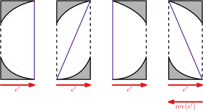
Figure 5: The connected components of $\Delta^{\prime}\mathchar 45\relax\mathrm{FSD}(e^{\prime},T)$ fall into these four cases, based on where the minima and maxima of the bottom and top parabolic arcs lie. In the first three cases, there is a clear matching with optimal coverage (purple). In the fourth case, the matching is only valid when mirroring the free space, achieved by using $\mathrm{rev}(e^{\prime})$ instead of $e^{\prime}$.

Applying the construction to all edges of $S$ and comparing the coverage, we obtain a prefix pathlet with the desired quality. This pathlet is a prefix or suffix pathlet with respect to one of the $\mathcal{O}(|S|\cdot n)$ subsegments obtained by subdividing all edges of $S$ in the above manner. This means that the intervals in the resulting pathlet all have endpoints that come from a set of $\mathcal{O}(n^{4})$ values, a linear factor more than was the case for prefix and suffix pathlets with respect to $S$. We hence obtain:

Theorem 9.4.

Let $C$ be a set of pathlets. In $\mathcal{O}(n^{3}\log^{2}n)$ time and using $\mathcal{O}(n^{2}\log n)$ space, we can construct a $(2,\Delta^{\prime})$-pathlet $(P,\mathcal{I})$ with

$$\lVert\mathrm{Cov}(P,\mathcal{I})\setminus\mathrm{Cov}(C)\rVert\geq\frac{1}{4}\lVert\mathrm{Cov}(P^{\prime},\mathcal{I}^{\prime})\setminus\mathrm{Cov}(C)\rVert$$

for any subedge $(2,\Delta^{\prime})$-pathlet $(P^{\prime},\mathcal{I}^{\prime})$. The intervals in $\mathcal{I}$ all have endpoints that come from a set of $\mathcal{O}(n^{4})$ values.

10 Constructing a pathlet-preserving simplification

10.1 Defining our $2\Delta$-simplification $S$

We consider the vertex-restricted simplification defined by Agarwal et al. [2] and generalize their $2\Delta$-simplification definition, allowing vertices to lie anywhere on $T$ (whilst still appearing in order along $T$). This way, we obtain a simplification with at most as many vertices as the optimal unrestricted $\Delta$-simplification (see Figure 6).

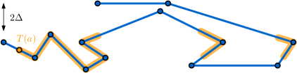
Figure 6: Consider the trajectory $T$ and some point $T(a)$. For some $\Delta$, we can indicate all $T(b)\in T$ with $a\leq b$ where for line $s=\overline{T(a)T(b)}$, $d_{F}(s,T[a,b])\leq 2\Delta$. Note that this set $\mathbb{B}(a)$ is not a connected set of intervals on $[1,n]$.

Definition 10.1.

Let $T$ be a trajectory with $n$ vertices, $\Delta\geq 0$ and $a\in[1,n]$. We define the set $\mathbb{B}(a)=\{b\geq a\mid d_{F}(\overline{T(a)T(b)},T[a,b])\leq 2\Delta\}$.

Definition 10.2.

Let $T$ be a trajectory with $n$ vertices and $\Delta\geq 0$. We define our $2\Delta$-simplified curve $S$ as follows: the first vertex of $S$ is $T(1)$. The second vertex of $S$ may be any point $T(a)$ with $a$ as a rightmost endpoint of an interval in $\mathbb{B}(1)$. The third vertex of $S$ may be any point $T(b)$ with $b$ as a rightmost endpoint of an interval in $\mathbb{B}(a)$, and so forth.

Per definition of the set $\mathbb{B}(a)$, the resulting curve $S$ is a $2\Delta$-simplified curve. We prove that $S$ is a pathlet-preserving simplification:

Lemma 10.3.

The curve $S$ as defined above is a pathlet-preserving simplification.

Proof 10.4.

The curve $S$ is a curve-restricted $2\Delta$-simplification and thus has Property (a). Next we show that for any subcurve $T[a,b]$ and all curves $P$ with $d_{F}(P,T[a,b])\leq\Delta$, the subcurve $S[s,t]$ (with $[s,t]=M^{TZ}([a,b])$) has complexity $|S[s,t]|\leq|P|+2-|\mathbb{N}\cap\{s,t\}|$. For brevity, we write $X=T[a,b]$. Fix any curve $P$ with $d_{F}(P,X)\leq\Delta$. There exists a $\Delta$-matchings $(M^{PX},M^{XP})$. Let $[s,t]=M^{TS}[a,b]$. Per construction, the subcurve $S[s,t]$ has Fréchet distance $d_{F}(S[s,t],X)\leq 2\Delta$ to $X$.

Any vertex of $T$ that is also a vertex of $S[s,t]$ is also a vertex of $T[a,b]$. Let $S[x,y]$ be the maximal vertex-subcurve of $S[s,t]$. This curve naturally has $|S[s,t]|-2+|\mathbb{N}\cap\{s,t\}|$ vertices. We argue that $|P|\geq|S[x,y]|$.

We introduce a slight abuse of notation. For a (sub) edge $e_{1}=S[i,i^{\prime\prime}]$ of $S$, we denote $M^{ST}(e)=M^{ST}([i,i^{\prime\prime}]$. Similarly, for a (sub) edge $e=P[j,j^{\prime\prime}]$ of $P$ we denote $M^{PX}(e)=M^{PX}([j,j^{\prime\prime}]$. Since $S$ is a $2\Delta$-simplification and $S[x,y]$ is a vertex-subcurve, we have for each edge $e_{1}$ of $S$ that $e_{1}=\overline{T(\alpha)T(\beta)}$ and $[\alpha,\beta]=M^{ST}(e_{1})$. Moreover, all intervals $[\alpha,\beta]$ together cover $[a,b]$.

Consider also for each edge $e\in P$ the interval $[c,d]=M^{PX}(e)$. All intervals $[c,d]$ together cover $[a,b]$. Suppose for the sake of contradiction that $|P|<|S[x,y]|$, then via the pigeonhole principle there exists at least one edge $e_{1}=\overline{T(\alpha)T(\beta)}$ of $S[x,y]$ and an edge $e$ of $P$ where $M^{PX}(e)=[c,d]$ with $c\leq\alpha\leq\beta<d$. We claim that for all $\beta^{\prime}\leq d$, $\beta^{\prime}\in\mathbb{B}(\alpha)$.

The proof is illustrated by Figure 7. For any $\beta^{\prime}\leq d$ there exists a sub-edge $e^{\prime}=e[x_{1},x_{2}]$ of $e$ where $M^{PX}(e^{\prime})=[\alpha,\beta^{\prime}]$. Per definition of a $\Delta$-matching we have that $d_{F}(T[\alpha,\beta^{\prime}],e^{\prime})\leq\Delta$. The $\Delta$-matching implies that

$$d(e^{\prime}(0),T(\alpha)),d(e^{\prime}(1),T(\beta^{\prime})))\leq\Delta.$$

We use this fact to apply [2, Lemma 3.1] and note that $d_{F}(e^{\prime},\overline{T(\alpha)T(\beta^{\prime})})\leq\Delta$. Applying the triangle inequality, we conclude that $d_{F}(T[\alpha,\beta^{\prime}],\overline{T(a)T(b^{\prime})})\leq 2\Delta$. It follows that for all $\beta^{\prime}\in[\alpha,d]$, $\beta^{\prime}\in\mathbb{B}(\alpha)$. This implies that $[\alpha,d]$ is contained in the first connected component of $\mathbb{B}(\alpha)$. However, per construction of $S$, $\beta$ is a rightmost endpoint of a connected component in $\mathbb{B}(\beta)$. This contradicts the fact that $\beta\in[\alpha,d)$.

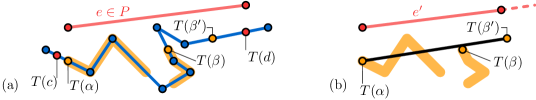
Figure 7: (a) The construction in the proof of Lemma 10.3. We have an edge $e$ with $d_{F}(e,T[c,d])\leq\Delta$. Moreover, for some $\alpha\in[c,d]$ we show $\mathbb{B}(\alpha)$ in orange where $\beta$ is the last value in some connected component of $\mathbb{B}(\alpha)$. (b) For any $\beta^{\prime}\in[\alpha,d]$, there exists a sub-edge $e^{\prime}$ of $e$ with $d_{F}(e^{\prime},T[a,\beta^{\prime}])\leq\Delta$.

10.2 Constructing the simplification

We give an $\mathcal{O}(n\log n)$ time algorithm for constructing our greedy simplification $S$ (Definition 10.2). Given any point $T(a)$ on $T$, we decompose the problem of finding a $b\in\mathbb{B}(a)$ over all edges of $T$. That is, given an $a\in[1,n]$, we consider an individual edge $T[i,i+1]$ of $T$. We show how to report the maximal $b\in[i,i+1]\cap\mathbb{B}(a)$. Our procedure is based off of the work by Guibas et al. [18] on ordered stabbing of disks in $\mathbb{R}^{2}$, and takes $\mathcal{O}(i-a)$ time. We fix a plane $H$ in $\mathbb{R}^{d}$ that contains $T(a)$ and $T[i,i+1]$. On a high-level, we apply the argument by Guibas et al.in $\mathbb{R}^{d}$ by restricting the disks to their intersection with $H$:

Definition 10.5.

Let $H$ be some fixed two-dimensional plane in $\mathbb{R}^{d}$. For any $x\in[1,n]$ denote by $B_{x}$ be the ball in $H$ that is obtained by intersecting a ball of radius $2\Delta$ centered at $T(x)$ with $H$. For $a\leq b$ we say that a directed line segment $e$ in $H$ stabs all balls in $[a,b]$ in order if for all $k\in\{a\}\cup([a,b]\cap\mathbb{N})\cup\{b\}$ there are points $p_{k}\in e\cap B_{k}$ such that $p_{k}$ comes before $p_{k^{\prime}}$ on $e$ whenever $k\leq k^{\prime}$ (see Figure 8 (a)).

Lemma 10.6 ([18, Theorem 14]).

A line segment $e$ is within Fréchet distance $2\Delta$ of a subcurve $T[a,b]$ of $T$ if and only if the following conditions are met:

1. $e$ starts within distance $2\Delta$ of $T(a)$,

2. $e$ ends within distance $2\Delta$ of $T(b)$, and

3. $e$ stabs all balls in $[a,b]$ in order.

Computing the maximal $b\in[i,i+1]\cap\mathbb{B}(a)$.

For any edge $e=\overline{T(a)T(b)}$ of $Z$, the endpoints lie on $T$ and thus $e$ trivially satisfies the first two criteria. It follows that if we fix some $T(a)$ on $S$ and some edge $T[i,i+1]$, then the maximal $b\in[i,i+1]$ (with $b\geq a$) for which $\overline{T(a)T(b)}$ stabs balls $[a,b]$ in order is also the maximal $b\in[i,i+1]\cap\mathbb{B}(a)$. We consider the following (slightly reformulated) lemma by Guibas et al. [18]:

Lemma 10.7 ([18, Lemma 8]).

Let $[a_{j},b_{j}]$ be a sequence of intervals. There exist $p_{j}\in[a_{j},b_{j}]$ with $p_{j}\leq p_{k}$ for all $j\leq k$, if and only if there is no pair $j\leq k$ with $b_{k}<a_{j}$.

The above lemma is applicable to segments in $H$ stabbing balls in $H$. Indeed, consider all integers $j\in[a,i]$. We may view any directed line segment $e$ in $H$ as (part of) the real number line, and view the intersections between $e$ and the disks $D_{j}$ as intervals. Lemma 10.7 then implies that $e$ stabs $[\lceil a\rceil,i]$ in order, if and only if no integers $j,k\in[a,i]$ exist with $j\leq k$ such that $e$ leaves $D_{k}$ before it enters $D_{j}$ (assuming $e$ intersects all disks).

For all integers $j\in[a,i]$, let $W_{j}:=\{p\in H\mid\overline{T(a)p}\textnormal{ intersects }D_{j}\}$. We define the stabbing wedge $\mathit{SW}_{j}:=\{p\in H\mid\overline{T(a)p}\textnormal{ intersects }[a,j]\textnormal{ in order}\}$. We prove the following:

Lemma 10.8.

Either $\mathit{SW}_{j}=\bigcap_{k\in[a,j]\cap\mathbb{N}}W_{k}$, or $\mathit{SW}_{j}=\emptyset$.

Proof 10.9.

The proof is by induction. The base case is that, trivially, $\mathit{SW}_{\lceil a\rceil}=W_{\lceil a\rceil}$. Any line $\overline{T(a)p}$ that intersects $[a,j]$ also intersects $[a,j-1]$, thus whenever $\mathit{SW}_{j-1}$ is empty, then $\mathit{SW}_{j}$ must also be empty. Suppose now that $\mathit{SW}_{j-1}=\bigcap_{k\in[a,j-1]\cap\mathbb{N}}W_{k}$. We show that $\mathit{SW}_{j}$ is either equal to $\mathit{SW}_{j-1}\cap W_{j}$, or it is empty (which, by induction, shows the lemma).

First we show that $\mathit{SW}_{j}\subseteq\mathit{SW}_{j-1}\cap W_{j}$. Suppose $\mathit{SW}_{j}$ is non-empty, and take a point $p\in\mathit{SW}_{j}$. By definition of stabbing wedge $\mathit{SW}_{j}$, the segment $\overline{T(a)p}$ stabs $[a,j]$ in order, and thus $[a,j-1]$ in order. Furthermore, $p$ must lie in $W_{j}$ for $\overline{T(a)p}$ to be able to stab disk $D_{j}$.

Next we show that $\mathit{SW}_{j-1}\cap W_{j}\subseteq\mathit{SW}_{j}$. By Lemma 10.7, $p\in\mathit{SW}_{j}$ if and only if $\overline{T(a)p}$ first enters all disks $D_{\lceil a\rceil},\dots,D_{j-1}$ before exiting disk $D_{j}$. Fix some $p\in\mathit{SW}_{j-1}\cap W_{j}$, for all $k<j$ the line $\overline{T(a)p}$ intersects $D_{k}$. If $p\neq\in\mathit{SW}_{j}$ then there must exist a $k<j$ where $\overline{T(a)p}$ exists $D_{j}$ before it enters $D_{k}$. The area $\mathit{SW}_{j-1}$ must be contained in the cone $C\subset H$ given by $T(a)$ and the two tangents of $D_{k}$ to $T(a)$ (Figure 8 (b)) and thus $\overline{T(a)p}$ is contained in $C$. Since $\overline{T(a)p}$ intersects $D_{k}$ in $C$ after $D_{j}$, it must be that $D_{j}\cap C$ is contained in a triangle $C^{*}$ formed by the boundary of $C$ and another tangent of $D_{k}$. However, this means that any segment $\overline{T(a)q}$ (for $q\in\mathit{SW}_{j-1}\cap W_{j})$ that stabs the disks $[a,j-1]$ in order must intersect $C^{*}$ before it intersects $D_{k}$. Thus, by Lemma 10.7, there is no segment $\overline{T(a)q}$ that stab the disks $[a,j]$ in order and $\mathit{SW}_{j}$ is empty.

Thus, either $\mathit{SW}_{j}$ is empty or $\mathit{SW}_{j}=\bigcap_{\lceil a\rceil\leq k\leq j}W_{k}$.

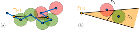
Figure 8: (a) For two points $T(a)$ and $T(b)$ on $T$, we consider all $j\in[a,b]\cap N$ and draw a ball with radius $2\Delta$ around them in green. (b) For all $k\in[a,j-1]\cap\mathbb{N}$, the area $\mathit{SW}_{j-1}$ must be contained in the orange cone.

Lemma 10.10.

Given $a\in[1,n]$ and edge $T[i,i+1]$ of $T$, we can compute the maximum $b\in[i,i+1]\cap\mathbb{B}(a)$, or report that no such $b$ exists, in $\mathcal{O}(1+i-a)$ time.

Proof 10.11.

By Lemma 10.6 (and the fact that $T(a)$ and $T(b)$ always lie on $T$) $b\in[i,i+1]\cap\mathbb{B}(a)$ if and only if $T(b)\in\mathit{SW}_{i}$. For any edge $T[i,i+1]$, we compute the maximal $b\in[i,i+1]\cap\mathbb{B}(a)$ by first assuming that $\mathit{SW}_{i}$ is non-empty. We check afterwards whether this assumption was correct, and if not, we know that no $b\in[i,i+1]$ exists with $d_{F}(T[a,b],\overline{T(a)T(b)})\leq 2\Delta$.

For all $j\in[a,i]\cap N$, we compute the last value $b_{j}\in[i,j]$ such that $T(b_{j})\in W_{j}$. This can be done in $\mathcal{O}(1)$ time per integer $j$, as wedges in the plane are formed by two rays and a circular arc in $H$, which we can intersect in $\mathcal{O}(1)$ time. Then we set $b=\min_{j}b_{j}$.

To check whether $\mathit{SW}_{i}$ is non-empty, we determine if $d_{F}(T[a,b],\overline{T(a)T(b)})\leq 2\Delta$. This takes $\mathcal{O}(1+i-a)$ time with the algorithm of Alt and Godau [5]. The assumption that $\mathit{SW}_{i}$ is non-empty is correct precisely if $d_{F}(T[a,b],\overline{T(a)T(b)})\leq 2\Delta$. If $\mathit{SW}_{i}$ is empty, $[i,i+1]\cap\mathbb{B}(a)$ is empty and no output exists. If $\mathit{SW}_{i}$ is non-empty, then by Lemma 10.8, the $b$ we choose is the maximal $b\in[i,i+1]\cap\mathbb{B}(a)$.

Lemma 10.12.

Given $a\in[1,n]$, we can compute a value $b^{*}$ that is the maximum of some connected component of $\mathbb{B}(a)$ in $\mathcal{O}((1+b^{*}-a)\log n)$ time.

Proof 10.13.

We use Lemma 10.10 in conjunction with exponential and binary search to compute the maximum $b^{*}$ of some connected component of $\mathbb{B}_{2\Delta}(a)$:

We search over the edges $T[i,i+1]$ of $T$. For each considered edge we apply Lemma 10.10 which returns some $b\in[i,j+1]\cap\mathbb{B}(a)$ (if the set is non-empty). We consider three cases:

If $b\in[i,i+1)$, then this value is the maximum of some connected component of $\mathbb{B}(a)$. We stop the search and output $b$.

If the procedure reports the value $b=i+1$ then this value may not necessarily be the maximum of a connected component. However, there is sure to be a maximum of at least $b$. Hence we continue the search among later edges of $T$ and discard all edges before, and including, $T[i,i+1]$.

If the procedure reports no value then $[i,i+1]\cap\mathbb{B}(a)=\emptyset$. Since trivially $a\in\mathbb{B}(a)$, it must be that there is a connected component whose maximum is strictly smaller than $i$. We continue the search among earlier edges of $T$ and discard all edges after, and including, $T[i,i+1]$.

The above algorithm returns the maximum $b^{*}\in[i^{*},i^{*}+1)$ of some connected component of $\mathbb{B}(a)$. By applying exponential search first, the edges $T[i,i+1]$ considered all have $i\leq 2i^{*}-a$. Hence we compute $b^{*}$ in $\mathcal{O}((1+b^{*}-a)\log n)$ time.

We now iteratively apply Lemma 10.12 to construct our curve $S$. We obtain a $2\Delta$-matching $(M^{ST},M^{TS})$ by constructing separate matchings between the edges $\overline{T(a)T(b)}$ of $S$ and the subcurves $T[a,b]$ that they simplify. By Lemma 10.3 this gives a pathlet-preserving simplification $(S,M^{ST},M^{TS})$.

See 5.4

References

- [1] Pankaj K. Agarwal, Kyle Fox, Kamesh Munagala, Abhinandan Nath, Jiangwei Pan, and Erin Taylor. Subtrajectory clustering: Models and algorithms. In proc. 37th ACM SIGMOD-SIGACT-SIGAI Symposium on Principles of Database Systems (PODS), pages 75–87, 2018. doi:10.1145/3196959.3196972.
- [2] Pankaj K. Agarwal, Sariel Har-Peled, Nabil H. Mustafa, and Yusu Wang. Near-linear time approximation algorithms for curve simplification. Algorithmica, 42(3):203–219, 2005. doi:10.1007/s00453-005-1165-y.
- [3] Hugo A. Akitaya, Frederik Brüning, Erin Chambers, and Anne Driemel. Subtrajectory clustering: Finding set covers for set systems of subcurves. Computing in Geometry and Topology, 2(1):1:1–1:48, 2023. doi:10.57717/cgt.v2i1.7.
- [4] Helmut Alt and Michael Godau. Computing the Fréchet distance between two polygonal curves. International Journal of Computational Geometry & Applications, 5:75–91, 1995. doi:10.1142/S0218195995000064.
- [5] Helmut Alt and Michael Godau. Computing the Fréchet distance between two polygonal curves. International Journal of Computational Geometry & Applications, 05(01n02):75–91, 1995. doi:10.1142/S0218195995000064.
- [6] Frederik Brüning, Jacobus Conradi, and Anne Driemel. Faster approximate covering of subcurves under the fréchet distance. In proc. 30th Annual European Symposium on Algorithms (ESA), volume 244 of Leibniz International Proceedings in Informatics (LIPIcs), pages 28:1–28:16, Dagstuhl, Germany, 2022. doi:10.4230/LIPIcs.ESA.2022.28.
- [7] Kevin Buchin, Maike Buchin, David Duran, Brittany Terese Fasy, Roel Jacobs, Vera Sacristan, Rodrigo I. Silveira, Frank Staals, and Carola Wenk. Clustering trajectories for map construction. In proc. 25th ACM SIGSPATIAL International Conference on Advances in Geographic Information Systems, pages 1–10, 2017. doi:10.1145/3139958.3139964.
- [8] Kevin Buchin, Maike Buchin, Joachim Gudmundsson, Jorren Hendriks, Erfan Hosseini Sereshgi, Vera Sacristán, Rodrigo I. Silveira, Jorrick Sleijster, Frank Staals, and Carola Wenk. Improved map construction using subtrajectory clustering. In proc. 4th ACM SIGSPATIAL Workshop on Location-Based Recommendations, Geosocial Networks, and Geoadvertising, pages 1–4, 2020. doi:10.1145/3423334.3431451.
- [9] Kevin Buchin, Maike Buchin, Joachim Gudmundsson, Maarten Löffler, and Jun Luo. Detecting commuting patterns by clustering subtrajectories. International Journal of Computational Geometry & Applications, 21(03):253–282, 2011. doi:10.1142/S0218195911003652.
- [10] Kevin Buchin, Anne Driemel, Joachim Gudmundsson, Michael Horton, Irina Kostitsyna, Maarten Löffler, and Martijn Struijs. Approximating -center clustering for curves. In proc. Thirtieth Annual ACM-SIAM Symposium on Discrete Algorithms (SODA), pages 2922–2938, 2019.
- [11] Maike Buchin and Dennis Rohde. Coresets for -median clustering under the Fréchet distance. In proc. Conference on Algorithms and Discrete Applied Mathematics, pages 167–180, 2022.
- [12] Siu-Wing Cheng and Haoqiang Huang. Curve simplification and clustering under Fréchet distance. In proc. 2023 Annual ACM-SIAM Symposium on Discrete Algorithms (SODA), pages 1414–1432, 2023.
- [13] Vasek Chvátal. A greedy heuristic for the set-covering problem. Mathematics of Operations Research, 4(3):233–235, 1979. doi:10.1287/MOOR.4.3.233.
- [14] Jacobus Conradi and Anne Driemel. Finding complex patterns in trajectory data via geometric set cover. arXiv preprint arXiv:2308.14865, 2023.
- [15] Mark de Berg, Atlas F. Cook, and Joachim Gudmundsson. Fast Fréchet queries. Computational Geometry, 46(6):747–755, 2013. doi:10.1016/j.comgeo.2012.11.006.
- [16] Anne Driemel, Amer Krivošija, and Christian Sohler. Clustering time series under the Fréchet distance. In proc. twenty-seventh annual ACM-SIAM symposium on Discrete algorithms (SODA), pages 766–785, 2016.
- [17] Joachim Gudmundsson and Sampson Wong. Cubic upper and lower bounds for subtrajectory clustering under the continuous Fréchet distance. In proc. 2022 Annual ACM-SIAM Symposium on Discrete Algorithms (SODA), pages 173–189, 2022.
- [18] Leonidas J. Guibas, John Hershberger, Joseph S. B. Mitchell, and Jack Snoeyink. Approximating polygons and subdivisions with minimum link paths. International Journal of Computational Geometry & Applications, 3(4):383–415, 1993. doi:10.1142/S0218195993000257.
- [19] Jacob Holm, Eva Rotenberg, and Mikkel Thorup. Planar reachability in linear space and constant time. In proc. IEEE 56th Annual Symposium on Foundations of Computer Science (FOCS), pages 370–389. IEEE Computer Society, 2015. doi:10.1109/FOCS.2015.30.
- [20] Richard M. Karp. Reducibility among combinatorial problems. In proc. Symposium on the Complexity of Computer Computations, The IBM Research Symposia Series, pages 85–103, 1972. doi:10.1007/978-1-4684-2001-2\_9.
- [21] Mees van de Kerkhof, Irina Kostitsyna, Maarten Löffler, Majid Mirzanezhad, and Carola Wenk. Global curve simplification. European Symposium on Algorithms (ESA), 2019.
- [22] Peter Widmayer. On graphs preserving rectilinear shortest paths in the presence of obstacles. Annals of Operations Research, 33(7):557–575, 1991. doi:10.1007/BF02067242.