An Improved Lower Bound on the Number of Pseudoline Arrangements

Abstract

Arrangements of pseudolines are classic objects in discrete and computational geometry. They have been studied with increasing intensity since their introduction almost 100 years ago. The study of the number $B_{n}$ of non-isomorphic simple arrangements of $n$ pseudolines goes back to Goodman and Pollack, Knuth, and others. It is known that $B_{n}$ is in the order of $2^{\Theta(n^{2})}$ and finding asymptotic bounds on $b_{n}=\frac{\log_{2}(B_{n})}{n^{2}}$ remains a challenging task. In 2011, Felsner and Valtr showed that $0.1887\leq b_{n}\leq 0.6571$ for sufficiently large $n$. The upper bound remains untouched but in 2020 Dumitrescu and Mandal improved the lower bound constant to $0.2083$. Their approach utilizes the known values of $B_{n}$ for up to $n=12$.

We tackle the lower bound with a dynamic programming scheme. Our new bound is $b_{n}\geq 0.2526$ for sufficiently large $n$. The result is based on a delicate interplay of theoretical ideas and computer assistance.

1 Introduction

Levi [19] introduced arrangements of pseudolines as a natural generalization of line arrangements in 1926. Ringel studied them in the 1950’s and Grünbaum [16] popularized them in his 1972 monograph Arrangements and Spreads. In the 1980’s Goodman and Pollack initiated a thorough study and related them to many other objects of interest in discrete geometry. For a more detailed account to the history and the relevant references we refer the interested reader to the handbook article [12].

An arrangement of pseudolines in the Euclidean plane $\mathbb{R}^{2}$ is a finite family of simple curves, called pseudolines, such that each curve approaches infinity in both directions and every pair intersects in exactly one point where the two curves cross. More generally, we call a collection of pseudolines partial arrangement if every pair intersects in at most one crossing-point. Pseudolines which do not intersect are said to be parallel. Note that, while for partial arrangements of proper lines the relation ’parallel’ is transitive, this is no longer true in partial pseudoline arrangements.

In this article, the focus will be on simple arrangements, that is, no three or more pseudolines intersect in a common point (called multicrossing). Moreover, we consider all arrangements to be marked, that is, they have a unique marked unbounded cell, which is called north-cell. Two arrangements are isomorphic if one can be mapped to the other by an orientation preserving homeomorphism of the plane that also preserves the north-cell.

While it is known that the number $B_{n}$ of non-isomorphic arrangements of $n$ pseudolines grows as $2^{\Theta(n^{2})}$, it remains a challenging problem to bound the multiplicative factor of the leading term of $\log_{2}B_{n}=\Theta(n^{2})$. Determining precise values for small values of $n$ is a challenging task as well, see the sequence A006245 in the OEIS [22]. Our focus will be on finding better estimates on the lower bound constant $c^{-}:=\liminf_{n\to\infty}\frac{\log_{2}B_{n}}{n^{2}}$. One can analogously define the upper bound constant $c^{+}:=\limsup_{n\to\infty}\frac{\log_{2}B_{n}}{n^{2}}$. It seems to be open whether $c^{+}$ and $c^{-}$ coincide, i.e., whether the limit exists.

A lot of work has been done on finding good estimates for $c^{-}$ and $c^{+}$. In the 1980’s Goodman and Pollak [15] investigated pseudopoint configurations, which are dual to pseudoline arrangements, and established the lower bound $c^{-}\geq\frac{1}{8}$. An alternative and slightly easier construction for $c^{-}\geq\frac{1}{12}$ was given by Matoušek in his Lectures on Discrete Geometry [20, Chapter 6]. As pointed out in [9] one also obtains $c^{-}\geq\frac{1}{8}$ from Matoušek’s construction via recursion. Concerning the upper bound, Edelsbrunner, O’Rourke and Seidel [10] showed $c^{+}<\infty$ via an algorithm that constructs an arrangement of $n$ pseudolines in $O(n^{2})$ time. It is worth noting that an upper bound can also be obtained via planar graphs: The dual graph of arrangement of $n$ pseudolines is planar quadrangulation on $m=\binom{n}{2}+n+1$ vertices. Since the number of $m$-vertex planar graphs is at most $2^{O(m)}$ [5, 6], it follows that $B_{n}\leq 2^{O(n^{2})}$.

In the 1990’s Knuth [17, Section 9] improved the bounds to $c^{-}\geq\frac{1}{6}$ and $c^{+}<0.7925$, and he conjectured that $c^{+}\leq 0.5$. The upper bound was lowered to $c^{+}<0.6974$ by Felsner [11]. In 2011, Felsner and Valtr [14] further narrowed the gap by showing $c^{-}>0.1887$ and $c^{+}<0.6571$, and, in 2020 Dumitrescu and Mandal [9] proved the currently best lower bound $c^{-}>0.2083$.

In this article, we make a substantial step on the lower bound by proving $c^{-}>0.2526$.

Theorem 1.1.

The number $B_{n}$ of non-isomorphic simple arrangements of $n$ pseudolines satisfies the inequality $B_{n}\geq 2^{cn^{2}-O(n\log n)}$ with $c>0.2526$.

2 Outline

Our approach is in the spirit of several previous bounds. We consider a specific partial arrangement $\cal L$ of $n$ lines consisting of $k$ bundles $\mathcal{L}_{1},\ldots,\mathcal{L}_{k}$ of parallel lines. We then define a class of local perturbations to $\cal L$ and consider the number of arrangements that can be obtained by these perturbations. This number is a lower bound on $B_{n}$, and it can be improved by recursively applying the same construction to each of the parallel classes $\mathcal{L}_{i}$.

The main difference between the approaches lies in the number of bundles $k$ and the choice of locality. Matoušek and also Felsner and Valtr used three bundles but the locality was increased from considering just a triple intersection with its two simple resolutions to the full intersection pattern of three bundles. Dumitrescu and Mandal [9] increased the number $k$ of bundles to up to 12 but still restricted the locality to the possible resolutions of the multicrossings.

Our approach combines higher values of $k$ with an increased locality for the perturbations. While in previous literature perturbations were restricted to local resolutions of multicrossings, we allow reroutings of the arrangement within designated regions, which we call patches. Figure 1 gives an illustration.

When rerouting the arrangement within a patch $P$, the order of the crossings along the pseudolines may change. More specifically, a rerouting may swap two crossings along a pseudoline inside $P$; see e.g. Figure 1. As we discuss in Section 5, the boundary information of $P$ fully determines which pairs of pseudolines cross within $P$, but the order of crossings along the pseudolines is not determined in general. Outside of $P$, the arrangement remains unaffected, which allows us to count the number of reroutings for each patch independently. The total number of perturbations is obtained as the product of the numbers computed for the individual patches. Details on how we computed the number of possibilities within a patch are defered to Section 5.

To eventually use computer assistance, we choose patches of high regularity and reasonably small complexity. In fact, since our construction is highly regular, it is sufficient to determine the rerouting possibilities only for a small number of patch-types. Only a negligible fraction of patches along the boundaries are different. As we only want to find an asymptotic lower bound on $B_{n}$, the small number of irregular patches along the boundary of the regions will not be used in the counting.

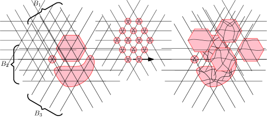
Figure 1: Left: An arrangement of $k=3$ bundles of parallel lines and a collection of interior-disjoint patches (highlighted red) such that each multicrossing point is covered by a patch. Right: A partial pseudoline arrangement with the same parallel bundles obtained by rerouting within the patches.

To eventually prove Theorem 1.1, we perform the following two steps:

• In the first step (Section 3) we specify the parameters of the construction: For $k=4$ and $k=6$, we construct $k$ bundles of ${\left\lfloor\frac{n}{k}\right\rfloor}$ parallel lines and cover the multicrossing points by patches. By resolving the multicrossing points within the patches, and taking the product over all patches we obtain an improved lower bound on the number $F_{k}(n)$ of partial arrangements with $k$ bundles of ${\left\lfloor\frac{n}{k}\right\rfloor}$ parallel pseudolines.

• In the second step (Section 4), we account for crossings in bundles of pseudolines which had been parallel before. The product of the so-computed possibilities yields the improved lower bound on the number $B_{n}$ of simple arrangements on $n$ pseudolines.

3 Step 1: bundles of parallel lines, patches, and perturbations

For the start we fix an integer $k$ and construct an arrangement $\mathcal{L}$ of $k$ bundles of ${\left\lfloor\frac{n}{k}\right\rfloor}$ parallel lines as in [9]. If $n$ is not a multiple of $k$, the remaining lines are discarded, or not used in the counting. We then cover all multicrossing points by a family of disjoint regions, called patches, and reroute the line segments within the patches so that all multicrossing points will eventually be resolved and the arrangement becomes simple. Since we use computers it is convenient to construct patches with a high regularity. Moreover, for simplicity in the computational part (cf. Section 5) we ensure that no crossings of $\mathcal{L}$ are located on the boundary of a patch and no patch has a touching with a line.

• Extremum 1: If we use one tiny patch for each of the multicrossings, the counting will give the same results as in [9], where each multicrossing was rerouted locally in all possible ways for various configurations with $k$ up to 12.

• Extremum 2: If we choose one gigantic patch containing all crossings of $\mathcal{L}$, then all partial arrangements of $n$ pseudolines with the same parallel bundles as in $\mathcal{L}$ will be counted, that is $F_{k}(n)$. For the case of $k=3$ bundles, Felsner and Valtr [14] determined that $F_{3}(n)=2^{cn^{2}+o(n^{2})}$ where $c=\frac{\log_{2}(3)}{2}-\frac{2}{3}\approx 0.1258$.

3.1 Construction with 4 bundles

First we construct a partial arrangement $\mathcal{L}$ of $n$ lines consisting of $4$ bundles of ${\left\lfloor\frac{n}{4}\right\rfloor}$ parallel lines $\mathcal{L}_{1},\ldots,\mathcal{L}_{4}$ following [9]. See Figure 2 for an illustration.

The construction comes with crossings of order 2, 3, and 4. We restrict our attention to regions with multicrossings since regions with 2-crossings do not allow further reroutings. As illustrated on the right-hand side figure, there are two types of regions with multicrossings:

• $R_{3}$ contains multicrossings of degree $3$ and

• $R_{4}$ contains multicrossings of degree $4$.

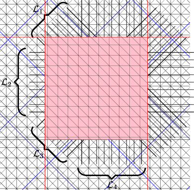
Figure 2: Construction with 4 bundles as in [9].

We use different patches in the regions $R_{3}$ and $R_{4}$ but in both cases rectangular patches can be used to tile the full region apart from a negligible area at its boundary, see Figure 3. Since the computing times depend on the complexity of the patch, we were able to use a geometrically larger patch to tile $R_{3}$. In Section 6 we discuss additional ideas on how to optimize the resulting bound.

(a)

(b)

Figure 3: The two types of patches for our construction on $k=4$ bundles:
3(a) For $R_{4}$ we use a rectangular tiling such that each patch $P_{4}$ contains exactly $8\cdot 4=32$ crossings of order 4.
3(b) For $R_{3}$ we use a rectangular tiling such that each patch $P_{3}$ contains exactly $10\cdot 10=100$ crossings of order 3.

Next we want to determine the number $\mu_{i}$ of patches of type $P_{i}$. Since the number of crossings in our construction is asymptotically quadratic in $n$ and each patch contains only a constant number of crossings, the number $\mu_{i}$ of patches of type $P_{i}$ is also quadratic. It is important to note that the patches along the boundary of $R_{i}$ behave differently. However, since there are only linearly many of these irregular patches, they only affect the lower order error term. Hence we can omit them in the calculations.

To obtain asymptotically tight estimates on the $\mu_{i}$’s, we make use of the numbers $\lambda_{i}(n)$ of $i$-crossing points, which have been determined by Dumitrescu and Mandal [9, page 66]:

• $\lambda_{3}(n)=\frac{1}{32}n^{2}-O(n)$

• $\lambda_{4}(n)=\frac{1}{32}n^{2}-O(n)$

For both, $i=3$ and $i=4$, the number $\lambda_{i}$ fulfills

$$\lambda_{i}=\mu_{i}\cdot\#\{\text{$i$-fold crossings in\leavevmode\nobreak\ $P_{i}$}\}+O(n)$$

because only the patch $P_{i}$ contains $i$-crossings. Consequently, we can determine the $\mu_{i}$’s after counting the numbers of crossings within our patches:

• $\mu_{3}(P_{3},n)=\frac{\lambda_{3}(n)}{\#\{\text{$3$-crossings in $P_{3}$}\}}-O(n)=\frac{n^{2}}{32\cdot 100}-O(n)$

• $\mu_{4}(P_{4},n)=\frac{\lambda_{4}(n)}{\#\{\text{$4$-crossings in $P_{4}$}\}}-O(n)=\frac{n^{2}}{32\cdot 32}-O(n)$.

Alternatively one can compute the $\mu_{i}$’s using the areas of the regions and patches without the indirection of the $\lambda_{i}$:

$$\mu_{i}=\frac{\operatorname{area}(R_{i})}{\operatorname{area}(P_{i})}-O(n),$$

where $\operatorname{area}(R_{i})$ denotes the area of the region $R_{i}$ and $\operatorname{area}(P_{i})$ denotes the area of a patch $P_{i}$.

To compute the numbers $F(P_{3})$ and $F(P_{4})$ of all possible reroutings within the patches of type $P_{3}$ and $P_{4}$, we ran our program and obtained:

• $F(P_{3})=1956055471674766249002559523437101670400$

• $F(P_{4})=10233480626615962155895931163981261674$.

We provide a computer-assisted framework [1] that can fully automatically compute $F(P)$ for a given patch $P$, which is given as an IPE input file [7]; see Section 5 for details. The presented terms were computed within a few CPU hours on cluster nodes of TU Berlin with up to 1TB of RAM. We also provide simpler patches for which the program only needs few CPU seconds and low RAM. Those, however, give slightly worse bounds.

Combining the possibilities from all the patches according to $F_{k}(n)\geq\prod_{i=3}^{k}F(P_{i})^{\mu_{i}(P_{i},n)}$ we obtain

Proposition 3.1.

$F_{4}(n)\geq 2^{cn^{2}-O(n)}$ with $c>0.1608$.

More specifically, by writing $c_{i}:=\lim_{n\to\infty}\frac{\mu_{i}(n)}{n^{2}}\cdot\log_{2}(F(P_{i}))$, we can see the contributions of the patches $P_{3}$ and $P_{4}$ to the leading constant $c=c_{3}+c_{4}$ from Proposition 3.1:

• $c_{3}\approx 0.0408$

• $c_{4}\approx 0.1201$.

3.2 Construction with 6 bundles

In this section we consider a partial arrangement $\mathcal{L}$ of $n$ lines consisting of $6$ bundles of ${\left\lfloor\frac{n}{6}\right\rfloor}$ parallel lines $\mathcal{L}_{1},\ldots,\mathcal{L}_{6}$. See Figure 4 for an illustration.

The construction comes with four types of regions with multicrossings:

• $R_{i}$ for $i\in\{3,4,5\}$ only contains multicrossings of order $i$ and

• $R_{6}$ contains multicrossings of order 3 and 6.

Note that in contrast to the $k=4$ bundle construction from Section 3.1, multicrossings of order 3 now occur in $R_{3}$ and $R_{6}$.

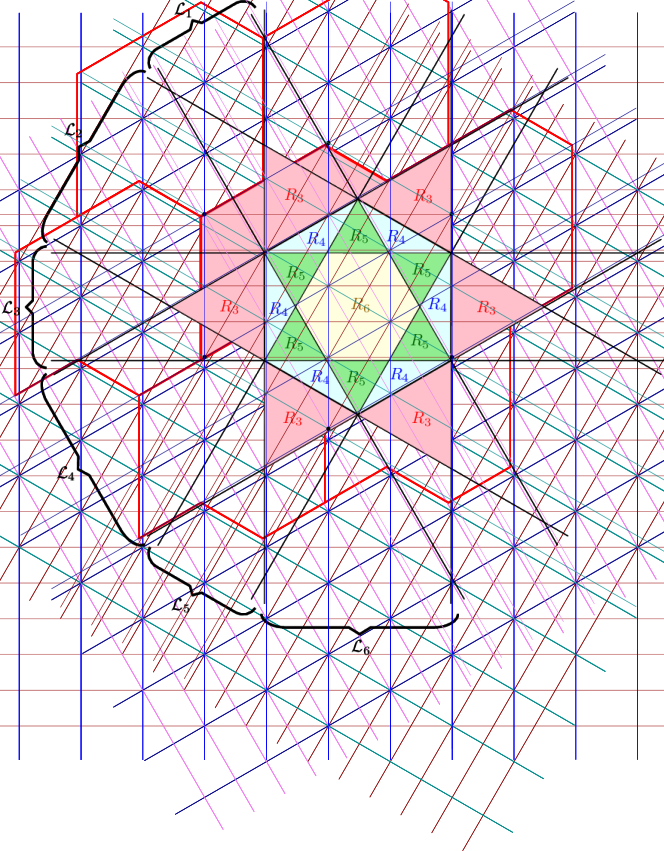
Figure 4: Construction with 6 bundles as in [9].

For each of the four regions $R_{i}$ we will use a different type of patch $P_{i}$ that is based on a regular tiling of the plane to ensure regularity; see Figure 5. Pause to note that $P_{3}$ and $P_{4}$ are affine transformations of the patches used in the 4 slopes setting in Section 3.1. Therefore they allow the same number of reroutings $F(P_{3})$ and $F(P_{4})$.

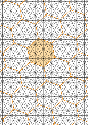
(a)

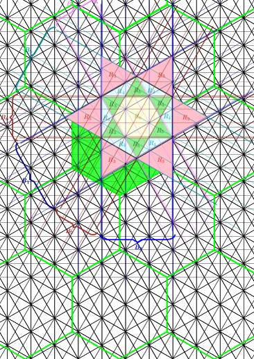
(b)

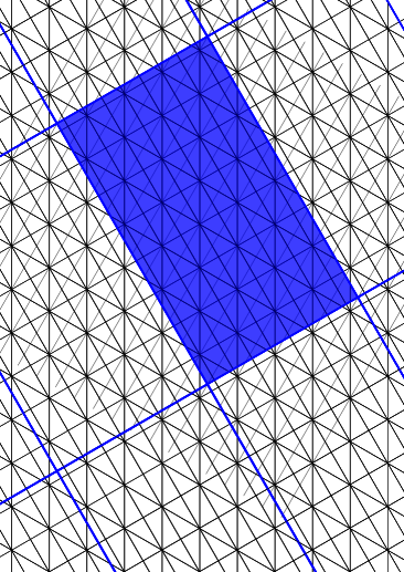
(c)

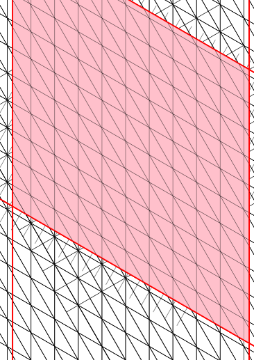
(d)

Figure 5: The four types of patches for our construction on $k=6$ bundles:
5(a) For $R_{6}$ we use a hexagonal tiling such that each patch $P_{6}$ contains exactly 7 crossings of order 6 and 14 crossings of order 3.
5(b) For $R_{5}$ we use a hexagonal tiling such that each patch $P_{5}$ contains exactly 12 crossings of order 5.
5(c) For $R_{4}$ we use a rectangular tiling such that each patch $P_{4}$ contains exactly $8\cdot 4=32$ crossings of order 4.
5(d) For $R_{3}$ we use a rhombic tiling such that each patch $P_{3}$ contains exactly $10\cdot 10=100$ crossings of order 3.

We have to determine the number $\mu_{i}$ of patches of type $i$. Since the number of crossings of each order is asymptotically quadratic in $n$ and each patch contains only a constant number of crossings, the number $\mu_{i}$ of patches of type $i$ is also quadratic. Again, it is important to note that the patches along the boundary of $R_{i}$ behave differently. However, since there are only linearly many of these deformed patches, they only affect lower order error terms. Hence we can omit them in the calculations.

To obtain asymptotically tight estimates on the $\mu_{i}$’s, we again make use of the numbers $\lambda_{i}(n)$ of $i$-crossing points, which have been determined by Dumitrescu and Mandal [9, Table 2]:

• $\lambda_{3}(n)=\frac{5}{144}n^{2}-O(n)$

• $\lambda_{4}(n)=\frac{1}{144}n^{2}-O(n)$

• $\lambda_{5}(n)=\frac{1}{144}n^{2}-O(n)$

• $\lambda_{6}(n)=\frac{1}{144}n^{2}-O(n)$

For $i=4,5,6$, the number $\lambda_{i}$ coincides with $\mu_{i}\cdot\#\{\text{$i$-fold crossings in\leavevmode\nobreak\ $P_{i}$}\}+O(n)$ because only the region $P_{i}$ contains $i$-crossings for $i=4,5,6$. For $i=3$, however, the situation is a bit more complicated because $P_{3}$ and $P_{6}$ both contains 3-crossings. More specifically, $P_{6}$ contains twice as many 3-crossings as 6-crossings. With the multiplicities given in the caption of Figure 5 we obtain:

• $\mu_{3}(P_{3},n)=\frac{\lambda_{3}(n)-2\cdot\lambda_{6}(n)}{\#\{\text{$3$-crossings in $P_{3}$}\}}-O(n)=\frac{3n^{2}}{144\cdot 100}-O(n)$

• $\mu_{4}(P_{4},n)=\frac{\lambda_{4}(n)}{\#\{\text{$4$-crossings in $P_{4}$}\}}-O(n)=\frac{n^{2}}{144\cdot 32}-O(n)$

• $\mu_{5}(P_{5},n)=\frac{\lambda_{5}(n)}{\#\{\text{$5$-crossings in $P_{5}$}\}}-O(n)=\frac{n^{2}}{144\cdot 12}-O(n)$

• $\mu_{6}(P_{6},n)=\frac{\lambda_{6}(n)}{\#\{\text{$6$-crossings in $P_{6}$}\}}-O(n)=\frac{n^{2}}{144\cdot 7}-O(n)$

To compute the numbers $F(P_{i})$ of all possible perturbations within the patch type $P_{i}$ for $i=3,4,5,6$, we ran our program and obtained:

• $F(P_{3})=1956055471674766249002559523437101670400$

• $F(P_{4})=10233480626615962155895931163981261674$

• $F(P_{5})=32207077855497546508132740267$

• $F(P_{6})=8129606100972933137253330355173$

We provide a computer-assisted framework [1] that can fully automatically compute $F(P)$ for a given patch $P$, which is given as an IPE input file [7]; see Section 5 for details. The presented terms were computed within a few CPU hours on cluster nodes of TU Berlin with up to 1TB of RAM. We also provide simpler patches for which the program only needs few CPU seconds and low RAM. Those, however, give slightly worse bounds.

From $F_{k}(n)\geq\prod_{i=3}^{k}F(P_{i})^{\mu_{i}(n)}$, we can now derive:

Proposition 3.2.

$F_{6}(n)\geq 2^{cn^{2}-O(n)}$ with $c>0.2105$.

More specifically, by writing $c_{i}:=\lim_{n\to\infty}\frac{\mu_{i}(n)}{n^{2}}\cdot\log_{2}(F(P_{i}))$, we can see the contributions of the patches $P_{3}$, $P_{4}$, $P_{5}$ and $P_{6}$ to the leading constant $c=c_{3}+c_{4}+c_{5}+c_{6}$ from Proposition 3.2:

• $c_{3}\approx 0.0272$

• $c_{4}\approx 0.0267$

• $c_{5}\approx 0.0548$

• $c_{6}\approx 0.1019$.

4 Step 2: resolving parallel bundles

With the second and final step, we want to obtain a simple arrangement of pairwise intersecting pseudolines from a partial arrangement of $k$ bundles of $m={\left\lfloor\frac{n}{k}\right\rfloor}$ parallel pseudolines. To do so, we use a recursive scheme as in [14, 9] to make each pair of parallel pseudolines cross: For each $i=1,\ldots,k$, we consider a disk $D_{i}$ such that

1. $D_{i}$ intersects all parallel pseudolines of the bundle $\mathcal{L}_{i}$ and no other pseudolines, and

2. no two disks overlap.

Within each disk $D_{i}$ we can place any of the $B_{m}$ arrangements of $m$ pseudolines. This makes all the pseudolines of a bundle cross. Figure 6 gives an illustration for the case $k=3$.

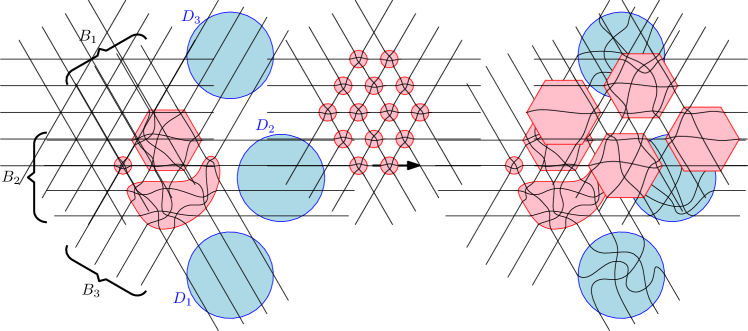
Figure 6: Left: A partial arrangement of $3$ bundles of parallel pseudolines and a collection of interior-disjoint disks (highlighted blue) such that each bundle is covered by one disk.
Right: A proper pseudoline arrangement obtained by rerouting within the disks.

Since all $D_{i}^{\prime}s$ are independent and there are $B_{m}$ possibilities to reroute within each $D_{i}$, we obtain the estimate

$$B_{n}\geq\underbrace{F_{k}(n)}_{\text{Step 1}}\cdot\underbrace{(B_{m})^{k}}_{\text{Step\leavevmode\nobreak\ 2}},$$

where $m={\left\lfloor\frac{n}{k}\right\rfloor}$. With the following lemma we can derive $c^{-}\geq\frac{k}{k-1}c$ where $c$ is the constant obtained in Section 3. While the construction with $k=4$ bundles yields $c^{-}>0.2144$, which is already an improvement to the previous best bound by Dumitrescu and Mandal [9], the construction with $k=6$ bundles allows an even bigger step: It gives the lower bound $c^{-}>0.2526$, and therefore completes the proof of Theorem 1.1.

Lemma 4.1.

If $F_{k}(n)\geq 2^{cn^{2}-O(n)}$ for some $c>0$ then $B_{n}\geq 2^{\frac{k}{k-1}cn^{2}-O(n\log n)}$.

Proof 4.2.

Choose $L>0$ as a sufficiently large constant such that $F_{k}(n)\geq 2^{cn^{2}-Ln}$ holds for all $n\geq 1$. We show by induction that $B_{n}\geq 2^{\tilde{c}n^{2}-G(n)}$ where $G(n):=\tilde{L}n\log_{k}(\tilde{L}n)$, $\tilde{L}:=L+2\tilde{c}$, and $\tilde{c}:=\frac{k}{k-1}\cdot c$. The base case $n\leq k$ is clearly satisfied if $L$ is chosen sufficiently large. For the induction step, we have

$$\log_{2}B_{n} \geq\log_{2}\left(F_{k}(n)\cdot(B_{m})^{k}\right)$$

$$=\log_{2}F_{k}(n)+k\log_{2}B_{m}$$

$$\stackrel{{\scriptstyle I.H.}}{{\geq}}(cn^{2}-Ln)+k\left(\tilde{c}m^{2}-G(m)\right)$$

$$\geq cn^{2}-Ln+\frac{\tilde{c}}{k}(n-k)^{2}-kG(m)$$

$$=\underbrace{(c+\frac{\tilde{c}}{k})}_{=\tilde{c}}n^{2}-\underbrace{(L+2\tilde{c})}_{=\tilde{L}}n-kG(m)+\underbrace{ck}_{\geq 0},$$

where $m={\left\lfloor\frac{n}{k}\right\rfloor}$. Since $kG(m)+\tilde{L}n\leq G(n)$ holds by definition, the statement follows.

5 Counting all possible reroutings in a patch

In this section we discuss how to compute the number $F(P)$ of all possible perturbations within a patch $P$ with boundary curve $C$. Since $C$ has no touching with any line, the intersection of $P$ with any line $L\in\mathcal{L}$ yields proper line segments. And because $C$ passes no crossings all the end points of segments are distinct. We can label the end points on $C$ according to the index of the resulting line segments and since every index occurs twice, we call the cyclic sequence of end points along $C$ a bipermutation. Note that in the case of a non-convex boundary curve $C$, the intersection of a line with $P$ consist of several segments, they have to be distingushed by distinct labels. Figure 7 gives an illustration.

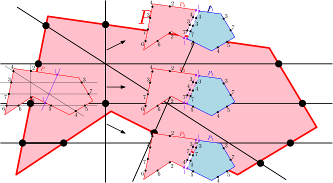
Figure 7: An illustration of how to recurse on a patch $P$. When cutting along segment $1$, highlighted purple, there are intersections with the segments $3$, $4$, and $7$. As the segments $3$ and $7$ do no cross within $P$, there are only three possibilities for placing the three crossings along the segment $1$, namely $4$–$3$–$7$ (right top), $3$–$4$–$7$ (right center) and $3$–$7$–$4$ (right bottom).

The number of possible reroutings within a patch $P$ is computed recursively: Choose a segment $z$, it splits $P$ into two parts. For every segment $a\neq z$ we can determine whether $a$ crosses $z$ by looking at the occurrences of $a$ and $z$ in the bipermutation. If up to cyclic shifts the pattern is $azaz$ they cross in $P$, if the pattern is $aazz$ they are parallel in $P$.

Now for every legal order $\pi$ of the crossing segments on $z$ we combine the two arcs of the bipermutation defined by the two occurrences of $z$ and combine them with $\pi$ to obtain the bipermutations of the two smaller patches $P_{1}$ and $P_{2}$. Figure 7 gives an example.

The legal orderings of crossings on $z$ can be found as follows: Consider a pair of segments $a,b$ that both cross $z$. $a$ and $b$ are either parallel in $P$ (i.e., we see $abzbaz$ in the bipermutation) or they form a crossing in $P$ which we denote by ${{a}\times{b}}$ (i.e., we see $abzabz$). In Figure 7 the segments $3$ and $7$ are parallel, and segments $3$ and $4$ cross, and the crossing point ${{3}\times{4}}$ can lie on either side of the segment $1$. In the case where $a$ and $b$ are parallel, the order of the two crossings ${{a}\times{z}}$ and ${{b}\times{z}}$ along $z$ is uniquely determined. In the case where $a$ and $b$ cross, the crossing point ${{a}\times{b}}$ can lie on either side of $z$, and the choice of the part further determines the order of the two crossings ${{a}\times{z}}$ and ${{b}\times{z}}$ along $z$. Altogether, the bipermutation of $P$ determines a partial order $\prec$ of all crossings on $z$ such that the legal orderings correspond to linear extensions of this partial ordering.

To count all possible reroutings within $P$, we iterate over all linear extensions $\prec^{\star}$ of $\prec$ and continue recursively. Note that linear extensions can be enumerated efficiently via back-tracking: pick a maximal element and recurse on the remaining elements. Each extension $\prec^{\star}$ uniquely determines the order of crossings along $z$ and therefore the two sides $P_{1}(z,\prec^{\star})$ and $P_{1}(z,\prec^{\star})$ can be explicitely given via their bipermutations. By cumulatively summing up the obtained numbers, we get

$$F(P)=\sum_{\text{$\prec^{\star}$ linear extension of $\prec$}}F(P_{1}(z,\prec^{\star}))\cdot F(P_{2}(z,\prec^{\star})).$$

We provide a computer-assisted framework [1] that allows to fully automatically compute $F(P)$ for a given patch $P$. The input is given as IPE-file. The program reads the collection of lines and the polygonal boundary of $P$, computes the bipermutation, and then performs a dynamic program to determine the number of reroutings within $P$. More specifically, we compute for each bipermutation the lexicographic minimal among all relabelings of the elements, and reuse previously computed values whenever possible.

6 Discussion

To obtain the best possible bound we performed quite some experiments to optimize the set of parameters. The resulting bound seems to be close to the best which could be obtained with parameters in the range of what is computable within modest time and space bounds on todays computers. Also it is important to note that as long as one fixes $k$, the counting approach is implicitly limited by $F_{k}(n)$, which is much smaller than $B_{n}$ because of possibilities to resolve the parallel bundles; see Section 4. Since $F_{3}(n)=2^{cn^{2}+o(n^{2})}$ with $c=\frac{\log_{2}(3)}{2}-\frac{2}{3}\approx 0.1258$ is known [14], it would be interesting to determine $\lim_{n\to\infty}\frac{\log_{2}F_{i}(n)}{n^{2}}$ for $i=4,\ldots,12$. In particular, we wonder how far from the truth the constant in Propositions 3.1 and 3.2 is.

To obtain the new lower bound constant $c^{-}>0.2526$ presented in Theorem 1.1, we started with the $k=6$ parallel bundles construction by Dumitrescu and Mandal [9] and covered the multicrossings with a specific selection of patches, which were inspired by regular tilings. While the results by Dumitrescu and Mandal suggest that larger values of $k$ give better bounds, the computations get more and more complex. In fact, as the number $k$ increases, the complexity of the patches increases. Since our program can only deal with patches containing about 30 to 40 segments in reasonable time, depending on the structure of crossings within it, there is a trade-off between the number of crossings within a patch and the number of bundles $k$ in practice. This was also the reason why we use different types of patch for the four regions (see Figure 5). In the future we plan to investigate also the construction with $k=8$ and $k=12$ bundles which as depicted in [9, Figures 9 and 13] come with more types of regions. To obtain a best possible bound, it remains a challenging part to find a good tiling/patches and for each of them.

There is also a lot of freedom for choosing the patches, and we indeed experimented with various shapes. The ones presented along Section 3 led to the best results. As mentioned along Section 5, when recursively computing $F(B)$, the choice of $z$ can have a significant impact on the computing time. Experiments showed that the best practical performance is obtained by choosing a cutting-segment $z$ such that

• the complexity of the larger part $P_{2}$ is as small as possible.

In practice this strategy tends to lead to

• balanced cuts, that is, $P_{1}$ and $P_{2}$ are of similar sizes;

• short cuts, that is, the number of intersections on $z$ is relatively small; and

• relatively small numbers of is legal orders.

In general each of those criteria may lead to a different cutting strategy. However, a properly balanced cut may come with larger parts and hence might be less efficient. Also the shortest cut will often be very unbalanced, resulting in one half that is only slightly smaller than the whole path and thus more recursion steps might be required to deal with the patch.

A good splitting strategy should also take the number of legal orders into account because a large number of legal orders will also negatively affect the computation time. The main advantage of our strategy is that it minimizes the complexity of both $P_{1}$ and $P_{2}$. This allows the algorithm to reach the bottom of recursive search tree as fast as possible. In practice it appeared to be more important to reach a low level in the search than to minimize the number of legal orders because the number of cache-hits (pre-computed values) increases fast as the level decreases. To obtain the best possible run-times on our configurations with $k=4$ and $k=6$ bundles, we performed benchmarks and made statistics for the computing time used in different layers in the recursive search tree. However, in general, it is hard to tell which cutting strategy is the best because we do not have any a priori estimates for the computation time or the number of reroutings for a patch.

Since local rerouting is a well-known and frequently used technique in combinatorial geometry, our technique might also be adapted to various other combinatorial structures to derive improved lower bounds. We see for example great potential for counting higher-dimensional pseudohyperplane arrangements, which are a natural generalization of pseudoline arrangements. More specifically, Ziegler constructed $2^{\Omega(n^{d})}$ arrangements of pseudohyperplanes in $\mathbb{R}^{d}$ [4, Theorem 7.4.2], and up to constant factors in the exponent, $2^{\Theta(n^{d})}$ is indeed best possible [4, Corollary 7.4.3]. With slight modification Ziegler’s construction even applies to the subclass of signotopes which corresponds to monotone colorings of hypergraphs [2, 3].

Here we also see potential for counting arrangements of pseudocircles [13] and simple drawings of the complete graph [21, 18].

References

- [1] Supplemental data. https://github.com/fcorteskuehnast/counting-arrangements.
- [2] Martin Balko. Ramsey numbers and monotone colorings. Journal of Combinatorial Theory, Series A, 163:34–58, 2019. doi:10.1016/j.jcta.2018.11.013.
- [3] Helena Bergold, Stefan Felsner, and Manfred Scheucher. An Extension Theorem for Signotopes. In 39th International Symposium on Computational Geometry (SoCG 2023), volume 258 of LIPIcs, pages 17:1–17:14. Schloss Dagstuhl, 2023. doi:10.4230/LIPIcs.SoCG.2023.17.
- [4] Anders Björner, Michel Las Vergnas, Bernd Sturmfels, Neil White, and Günter M. Ziegler. Oriented Matroids, volume 46 of Encyclopedia of Mathematics and its Applications. Cambridge University Press, 2 edition, 1999. doi:10.1017/CBO9780511586507.
- [5] Nicolas Bonichon, Cyril Gavoille, and Nicolas Hanusse. An information-theoretic upper bound of planar graphs using triangulation. In Annual Symposium on Theoretical Aspects of Computer Science (STACS 2003), pages 499–510. Springer, 2003. doi:10.1007/3-540-36494-3_44.
- [6] Nicolas Bonichon, Cyril Gavoille, and Nicolas Hanusse. An Information-Theoretic Upper Bound on Planar Graphs Using Well-Orderly Maps, pages 17–46. Birkhäuser, 2011. doi:10.1007/978-0-8176-4904-3_2.
- [7] Otfried Cheong. The Ipe extensible drawing editor. http://ipe.otfried.org/.
- [8] Fernando Cortés Kühnast. On the number of arrangements of pseudolines. Bachelor’s thesis, Technische Universität Berlin, Germany, 2023. https://fcorteskuehnast.github.io/files/bachelor_thesis.pdf.
- [9] Adrian Dumitrescu and Ritankar Mandal. New lower bounds for the number of pseudoline arrangements. Journal of Computational Geometry, 11:60–92, 2020. doi:10.20382/jocg.v11i1a3.
- [10] Herbert Edelsbrunner, Joseph O’Rourke, and Raimund Seidel. Constructing arrangements of lines and hyperplanes with applications. SIAM Journal on Computing, 15(2):341–363, 1986. doi:10.1137/0215024.
- [11] Stefan Felsner. On the Number of Arrangements of Pseudolines. Discrete & Computational Geometry, 18(3):257–267, 1997. doi:10.1007/PL00009318.
- [12] Stefan Felsner and Jacob E. Goodman. Pseudoline Arrangements. In C.D. Toth, J. O’Rourke, and J.E. Goodman, editors, Handbook of Discrete and Computational Geometry (3rd ed.). CRC Press, 2018. doi:10.1201/9781315119601.
- [13] Stefan Felsner and Manfred Scheucher. Arrangements of Pseudocircles: On Circularizability. Discrete & Computational Geometry, Ricky Pollack Memorial Issue, 64:776–813, 2020. doi:10.1007/s00454-019-00077-y.
- [14] Stefan Felsner and Pavel Valtr. Coding and Counting Arrangements of Pseudolines. Discrete & Computational Geometry, 46(3), 2011. doi:10.1007/s00454-011-9366-4.
- [15] Jacob E. Goodman and Richard Pollack. Multidimensional Sorting. SIAM Journal on Computing, 12(3):484–507, 1983. doi:10.1137/0212032.
- [16] Branko Grünbaum. Arrangements and Spreads, volume 10 of CBMS Regional Conference Series in Mathematics. AMS, 1972 (reprinted 1980). doi:10/knkd.
- [17] Donald E. Knuth. Axioms and Hulls, volume 606 of LNCS. Springer, 1992. doi:10/bwfnz9.
- [18] Jan Kynčl. Enumeration of simple complete topological graphs. European Journal of Combinatorics, 30(7):1676–1685, 2009. doi:10.1016/j.ejc.2009.03.005.
- [19] Friedrich Levi. Die Teilung der projektiven Ebene durch Gerade oder Pseudogerade. Berichte über die Verhandlungen der Sächsischen Akademie der Wissenschaften zu Leipzig, Mathematisch-Physische Klasse, 78:256–267, 1926.
- [20] Jiří Matoušek. Lectures on Discrete Geometry. Springer, 2002. doi:10.1007/978-1-4613-0039-7.
- [21] János Pach and Géza Tóth. How many ways can one draw a graph? Combinatorica, 26(5):559–576, 2006. doi:10.1007/s00493-006-0032-z.
-
[22]
Neil J. A. Sloane.
The on-line encyclopedia of integer sequences.
http://oeis.org.