Are boron-nitride nanobelts capable to capture greenhouse gases?

Abstract

Why is the question in the title pertinent? Toxic gases, which are detrimental to both human health and the environment, have been released in greater quantities as a result of industrial development. These gases necessitate capture, immobilization, and measurement. Consequently, the present study investigates the interactions between boron-nitride nanobelt and Möbius-type boron-nitride nanobelt and nine greenhouse gases, namely ammonia, carbon dioxide, carbon monoxide, hydrogen sulfide, methane, methanol, nitric dioxide, nitric oxide, and phosgene. The adsorption energies calculated for the structures with optimized geometry are all negative, suggesting that all gases are adsorbed favorably in both nanobelts. Furthermore, we discovered that the recovery time of the sensors ranges from two hours to a few nanoseconds, and that the nanobelts exhibit distinct responses to each gas. According to electronic and topological investigations, covalent bonds were exclusively formed by nitric oxide; the remaining gases formed non-covalent bonds. Molecular dynamics ultimately demonstrate that the interaction between a single gas molecule and the nanobelt remains consistent across the vast majority of gases, whereas the interaction between 500 gas molecules and the nanobelts functions as an attraction, notwithstanding the impact of volumetric effects characteristic of high volume gases on the interaction. For the completion of each calculation, semiempirical tight-binding methods were implemented utilizing the xTB software. The outcomes of our study generated a favorable response to the inquiry posed in the title.

1 Introduction

The escalation of industrialization, the improper disposal of waste and byproducts, and the combustion of fossil fuels have all contributed to an increase in environmental pollution [1; 2; 3]. Humans and the environment can be severely harmed by the emission of toxic gases, including phosgene, hydrogen sulfide, ammonia, nitric oxide, methanol, methane, carbon monoxide, and carbon dioxide [1].

Methanol (CH₃OH) is a hazardous alcohol that is frequently encountered in industrial and domestic byproducts. Prolonged exposure to it can result in severe illness and, in severe cases, fatalities [4]. In contrast, methane (CH₄) has the potential to cause harm due to its combustible nature when inhaled in excess [5]. Carbon monoxide (CO), an odorless, colorless, and tasteless gas, is produced when carbonaceous materials are incompletely burned [6; 7]. Victims frequently lose consciousness prior to becoming aware of the seriousness of their poisoning. Increased concentrations of carbon dioxide (CO₂) have the potential to negatively impact human health by displacing oxygen, resulting in toxicity via asphyxiation and acidosis. This can subsequently give rise to arrhythmias and damage to tissues [8]. Phosgene (COCl₂) exhibits a high degree of reactivity with functional groups present in the epithelium of the respiratory system, resulting in cellular deterioration [9; 10].

Hydrogen sulfide (H₂S) is an odorless, highly combustible gas that induces poisoning via inhalation; exposure to high concentrations results in fatal toxicity [11]. Ammonia (NH₃) is an exothermic gas that induces necrosis in body tissues via an exothermic reaction [12]. It is a highly toxic and irritating gas that causes severe tissue damage. Significant exposure to nitrogen oxide gases (NO and NO₂) can result in symptoms such as coughing, shortness of breath, and potentially even acute respiratory distress syndrome [13]. Additionally, NO₂ is capable of photochemically reacting with other pollutants to generate acid rain or ozone, thereby exacerbating its detrimental environmental impacts [1; 14]].

Due to the harmful effects of these gases, there is a necessity to monitor environmental pollution to ensure levels that do not harm living organisms [15; 16; 17]. Researchers have examined a range of gas detection systems and have determined that two-dimensional (2D) materials with their substantial surface area, adsorption specificity [18; 19], chemical stability [19; 20], and robust electrochemical performance [21; 19] may have substantial application potential. As an illustration, phosphorene has demonstrated efficacy in the detection of gases including NH₃, SO₂, NO, and NO₂ [22; 23]. Wu et al. [24] identified that by appending specific groups to arsenene, it becomes exceedingly efficient at locating molecules of CO, NO, NO₂, SO₂, NH₃, and H₂S. In addition, sensor materials capable of detecting gas molecules such as CO₂, CH₄, and N2 [25; 26] have been investigated in the context of two-dimensional materials, including graphene.

Carbon nanotubes, specifically, demonstrate considerable promise in the realm of novel gas separation apparatus development [27; 19]. For adsorbing gases such as CO₂ [28], CH₄ [29], and H₂ [30; 31; 19], single-walled carbon nanotubes (SWCNTs) have been utilized. Furthermore, investigations into the electronic characteristics of carbon nanotubes subsequent to the adsorption of gas molecules (NO₂, O₂, NH₃, N₂, CO₂, CH₄, H₂O, H₂, and Ar) have demonstrated that the electronic properties of SWCNTs are exceptionally susceptible to the adsorption of gases such as NO₂ and O₂ [19; 32]. Lu et al. additionally investigated the interactions between carbon nanobelt dimers (CNBs) and small gas molecules (N₂, CH₄, CO, CO₂, H₂, H₂O, H₂O₂, and O₂). They discovered that these molecules tend to be adsorbed more strongly inside the ring than outside, mainly because the interaction is much stronger [33].

Ahmed et al. conducted a recent study to assess the H₂S gas detection capability utilizing M¨bius carbon nanobelt strips (MCNBs), which demonstrated exceptional sensitivity towards the gases under investigation. Furthermore, the presence of negative entropy values indicated that each of the complex structures formed exhibited thermodynamic stability. In contrast, a more pronounced interaction with CH₄ gas was observed in the MCNB structure [17]. Such theoretical investigations aid in establishing a correlation between the interaction properties and structure of carbon nanomaterials. In addition, they provide theoretical guidance for practical implementations that aid in the development of sensors for specific gases [17]. Despite this, research on gas adsorption in various carbon structures is still limited. Therefore, computational modeling can serve as a crucial instrument in comprehending the underlying chemical and physical molecular mechanisms by furnishing pertinent data at the atomic level. When considering this, it is possible that properties obtained from diverse topologies could provide an alternative resolution to present-day issues like air pollution resulting from chemical contaminants, which negatively impact both the environment and living organisms [31; 17; 19].

In order to advance the domain of gas detection, it is imperative to establish interdisciplinary collaboration. Collaboration among engineers, physicists, chemists, and material scientists is imperative for the synthesis of novel materials, the characterization of their properties, and their integration into operational devices. Furthermore, by actively involving technology developers and policymakers, the process of translating laboratory discoveries into practical applications that protect the environment and public health can be facilitated.

Using semi-empirical tight-binding theory, the interactions of phosgene, nitric oxide, methanol, methane, carbon monoxide, carbon dioxide, phosgene, hydrogen sulfide, ammonia, and nitrogen dioxide with boron-nitride nanobelts were investigated in this study. Various methods were employed to characterize the systems: identifying the optimal interaction region, geometry optimization, molecular dynamics, electronic property calculations, and topology studies.

2 Materials and Methods

This study employed two distinct nanostructures composed of boron nitride (BN): a nanobelt and a Möbius nanobelt, also known as a twisted nanobelt. Beginning with two unit cells of a (10,0) boron-nitride nanosheet repeated ten times in the z-direction, the software Virtual NanoLab Atomistix Toolkit [34] generated the nanobelt. Subsequently, the nanobelt was wrapped in a 360 degree motion, the periodicity was eliminated, and the border atoms were passivated with hydrogen. In the case of Möbius nanobelt, after the initial repetition of the cells, the nanobelt was twisted 180 degrees and then wrapped. The following nine greenhouse gases were utilized: nitrogen-dioxide (NO₂), hydrogen-sulfide (H₂S), methanol (CH₃OH), methane (CH₄), carbon monoxide (CO), carbon dioxide (CO₂), phosgene (COCl₂), ammonia (NH₃), and nitrogen-oxide (NO). All the structures were neutrally charged and are shown in Figure 1.

The systems are designated with abbreviations BNNB and MBNNB to denote boron-nitride nanobelt and MBNNB, respectively, and BNNB+gas (MBNNB+gas) to denote the complexes formed between BNNB (MBNNB) and greenhouse gases, such as BNNB+NO. The initial structures and flowchart of the employed methodology are depicted in Figure 1.

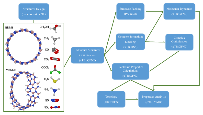
Figure 1: Initial structures and flowchart of the used methodology.

The calculations were conducted utilizing the xTB program’s implementation of the semiempirical tight binding method. The efficacy of the xTB package has been evaluated across multiple databases containing transition metals, organometallics, and lanthanide complexes. In comparison to techniques such as coupled cluster and Density Functional Theory (DFT), the xTB package produced exceptionally accurate outcomes [35; 36; 37; 38].

The calculations were performed in accordance with the sequence of procedures outlined in the methodology flowchart (refer to Figure 1). Initially, the structures of each individual system (consisting of two nanobelts and nine gases) were optimized. Following this, the docking process is completed utilizing automated Interaction Site Screening (aISS) [39]. Following a step that searches for pockets in molecule A (the nanobelts), a three-dimensional (3D) screening is performed to identify $\pi$-$\pi$ stacking interactions in various directions. Subsequently, approaches are made to identify the global orientations of molecule B (the gases) within an angular grid encircling molecule A. In order to rank the generated structures, the interaction energy (xTB-IFF) is utilized [40]. By default, for an additional two-step genetic algorithm optimization, one hundred structures with lower interaction energies are chosen. This ensures that conformations that were not detected in the initial screening are incorporated. In the course of this two-step genetic optimization procedure, each pair of positions of molecule B is randomly crossed around molecule A. Subsequently, 50% of the structures undergo random mutations in both position and angle. After ten iterations of this exhaustive search process, ten complexes with the lowest interaction energy are chosen. The structure with the lowest interaction energy is subsequently chosen as the input for the complex optimization.

The GFN2-xTB method, an exact self-consistent method that incorporates multipole electrostatics and density-dependent dispersion contributions [37], was utilized to optimize the geometry in its entirety. Extreme optimization level was ensured, with a convergence energy of $5\times 10^{-8}$ E_h and gradient norm convergence of $5\times 10^{-5}$ E_h/a₀ (where a₀ is the Bohr radius).

The electronic properties were calculated under the spin polarization scheme and included the system energy, the highest occupied molecular orbital energy (HOMO, $\varepsilon_{H}$), the lowest unoccupied molecular orbital energy (LUMO, $\varepsilon_{L}$), the energy gap between the HOMO and LUMO orbitals ($\Delta\varepsilon=\varepsilon_{H}-\varepsilon_{L}$), and the electron transfer integrals.

The change in the conductivity ($\Delta\sigma$) of a material leads to a change in the electric signal and can be used to measure the sensitivity of a sensor [41; 42]. These changes can be calculated as:

$$\Delta\sigma=(\sigma-\sigma_{0})/\sigma_{0},$$ (1)

where $\sigma_{0}$ and $\sigma$ are the isolated nanobelts and complex conductivities, respectively. As the conductivity of semiconductor material is proportional to the intrinsic carrier concentration (basically electrons) and their mobility, it is found that $\sigma$ is also proportional to the electronic gap as [43, p220]:

$$\sigma\propto Exp(-\Delta\varepsilon/2k_{B}T),$$ (2)

$k_{B}$ and $T$ are the Boltzmann constant and system temperature, respectively. Higher values of $\Delta\sigma$ indicate a higher sensitivity of the nanobelt to the corresponding gas.

To study the electron/hole mobility between the nanobelts and the absorbed gas molecules, we determine the electron transfer integrals, also known as coupling integrals, using the dimer projection (DIPRO) method [44]. Herein $J_{oc}$ represents the hole transport (occupied molecular orbitals), $J_{un}$ the electron transport (unoccupied molecular orbitals), and $J$ corresponds to the total charge transfer including the hole/electron transport between occupied/unoccupied molecular orbitals, respectively. Higher values of $J$ imply higher coupling between the two fragments (i.e., more intense interaction between them is).

From the total system energies, the adsorption energy ($E_{ads}$) of the gas molecules adsorbed on the nanobelts was calculated using the subsequent expression:

$$E_{ads}=E_{NB+gas}-E_{NB}-E_{gas}.$$ (3)

In equation 3, $E_{NB}$ and $E_{gas}$ are the energies for the isolated nanobelts and gas molecule, respectively, and $E_{NB+gas}$ is the energy of the NB+gas complex (BNNB+gas and MNBB+gas systems).

It is noteworthy to mention that very strong interactions are not favorable in gas detection because these imply that desorption of the adsorbate could be difficult and the device may suffer from long recovery times. The recovery time, one of the essential properties of gas-sensing materials, is exponentially related to the adsorption energy and was predicted using the transition theory as follows:

$$\tau=\nu^{-1}_{0}Exp(E_{ads}/k_{B}T)$$ (4)

where $\nu_{0}$ is the exposed used frequency. In this study, we estimated the recovery time using $\nu_{0}$=10¹² Hz (corresponding to ultraviolet radiation) and T=298.15 K.

Using the wave function obtained when calculating the electronic properties, the topological properties and descriptors (such as critical points, electronic density, Laplacian of the electronic density, etc.) were determined using the MULTIWFN [45] software.

As it is well known, geometry optimization involves using an algorithm to obtain a local minimum structure on the potential energy surface (PES), which allows us to determine the lowest energy conformers of a system. However, this method provides no information about the system’s stability over time. Molecular dynamics (MD) simulation, on the other hand, analyzes the movement of atoms and molecules at a specific temperature (here, 298.15 K) and provides a way to explore the PES.

We performed molecular dynamics in two different cases. In the first case, we perform simulations on each complex, starting with the structures obtained from the aISS step as initial conformations. This gave an idea about how one single gas molecule interacts with each nanobelt. In the second case, using the PACKMOL software [46; 47], we created initial complexes, adding 500 gas molecules to each nanobelt in a 20 Å radii spherical distribution as shown in Figure 2. This calculation gave information about how a more complex and realistic system evolved over time. Both molecular dynamics were run for a production time of 100 ps with a time step of 2 fs and an optional dump step of 50 fs, at which the final structure was written to a trajectory file. The molecular dynamics calculations were done using the GFN2-xTB method.

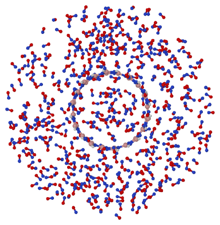
Figure 2: A BNNB packaged with 500 NO molecules in a spherical conformation of 20 Å radii. Image rendered with Jmol software [48] using the CPK color scheme.

To characterize the particle distribution of a heterogeneous system, the radial distribution function (RDF) can be used. The RDF denoted in equations by $g(r)$, is a pair correlation function that describes how, on average, the particles in a system are radially packed around each other [49] and can be calculated using expression 5:

$$g(\bf{r})=\frac{n(\bf{r})}{\rho 4\pi\bf{r}^{2}\Delta\bf{r}},$$ (5)

where $n(\bf{r})$ is the mean number of particles in a shell of width $\Delta\bf{r}$ at distance $\bf{r}$, and $\rho$ is the mean particle density.

The RDF ($g(\bf{r})$) not only describes the spatial correlation between two particles, but it can also be used to describe the potential of mean force [49]. This property indicates how the free energy changes as a function of some inter- or intramolecular coordinate and can be calculated as

$$W(\bf{r})=-k_{B}Tln[g(\bf{r})].$$ (6)

3 Results and discussion

3.1 Gas adsorption at the BN nanobelts

The calculated parameters for the geometry optimized complex are presented in Table 1 for the BNNB complexes and in Table 2 for the MBNNB complexes. In both tables, the data is presented in increasing order of the adsorption energy (lower negative values imply better/stronger adsorption). At first sight, all the gases presented negative adsorption energy, indicating a favorable interaction with both types of nanobelts. The NO, NH₃, CH₃OH, COCl₂, and NO₂ gases are in the top-5 interacting gases in common for both systems, BNNB and MBNNB. Nevertheless, a detailed analysis reveals that the Möbius boron-nitride-type nanobelt always presented lower values of the adsorption energies for all gases, ranging from 13% (NH₃) to 57% (CH₄) higher than the BNNB systems.

Even when the MBNNB has better adsorption energies for all gases than the BNNB, its sensitivity to each gas is different and not aligned with the values of $E_{ads}$. Changes in the material conductivity, $\Delta\sigma$, can be used to measure the material sensitivity when interacting with another molecule. As described by equation 1, the conductivity of a material is directly related to the electronic gap ($\Delta\varepsilon$) of the material. The reference conductivity, $\sigma_{0}$, is for the isolated nanobelts (without interacting with the gases). In tables 1 and 2, both values for $\Delta\varepsilon$ and $\Delta\sigma$ are shown. Positive (negative) $\Delta\sigma$ represents an increase (decrease) in the conductivity. The higher the value of $\Delta\sigma$ is, the more sensible the sensor is. Methane, CH₄, is the only gas that cannot be detected by either nanobelt, as its adsorption didn’t produce any change in the belt’s conductivity, e.g., $\Delta\sigma=0$. On the other hand, dissimilar values of $\Delta\sigma$ are good as they can be used as a parameter to measure the sensor specificity, i.e., given different electric responses for different adsorbed gases. Except for NH₃ and CH₃OH, which showed very similar variation in the conductivity for the BNNB, both nanobelts can be used not only as adsorbents, but also to detect the presence of each of the gases studied here.

As pointed out before, if it is intended to reuse the sensor, very strong interactions are not favorable, as the desorption of the adsorbate could be difficult. The re-usability of the sensor can be related to the time it takes to recover, i.e., remove the adsorbate. The sensor recovery time, $\tau$ is directly dependent on the adsorption energy and can be calculated using equation 4). Lower values of $\tau$ indicate that the gas can be easily detached from the nanobelt. As the BNNB system presents the highest $E_{ads}$, it presents the lowest values for $\tau$ ranging between a few seconds and a few nanoseconds. In the case of the MBNB, lower values of $E_{ads}$ implied the highest value of the recovery time, ranging from a thousand seconds to hundreds of nanoseconds. In all cases, the recovered times are feasible.

Table 1: Adsorption energy ($E_{ads}$), HOMO ($\varepsilon_{H}$), LUMO ($\varepsilon_{L}$), gap ($\Delta\varepsilon$), electrical conductivity variation ($\%\Delta\sigma$) by the adsorption, recovery time ($\tau$), and effective electron transfer integral ($J_{oc}$/$J_{un}$/$J$) for the BNNB systems^†.

System	$E_{ads}$	$\varepsilon_{H}$	$\varepsilon_{L}$	$\Delta\varepsilon$	$\%\Delta\sigma$	$\tau$	$J_{oc}$/$J_{un}$/$J$
BNNB	—	-9.503	-5.530	3.973	—	—	—
BNNB+NO	-0.768	-8.113	-5.759	2.354	292	16.46 s	—
BNNB+NH3	-0.650	-9.496	-5.555	3.941	3	0.15 s	4/6/8
BNNB+CH3OH	-0.481	-9.503	-5.559	3.944	2	187.09 $\mu$s	12/22/170
BNNB+COCl2	-0.476	-9.519	-8.071	1.447	743	156.78 $\mu$s	130/54/239
BNNB+NO2	-0.394	-9.416	-7.662	1.755	551	5.95 $\mu$s	—
BNNB+H2S	-0.284	-9.496	-5.595	3.901	6	76.07 ns	12/2/14
BNNB+CO2	-0.270	-9.520	-5.926	3.594	38	44.38 ns	6/23/21
BNNB+CO	-0.261	-9.519	-6.852	2.667	201	31.43 ns	20/4/48
BNNB+CH4	-0.134	-9.505	-5.532	3.973	0	0.20 ns	11/8/17

^† $E_{b}$ is in units kcal/mol; $\varepsilon_{H}$, $\varepsilon_{L}$, $\Delta\varepsilon$, are in units of $eV$ and $J_{oc}$, $J_{un}$, and $J$ are in units of $meV$.

Table 2: Adsorption energy ($E_{ads}$), HOMO ($\varepsilon_{H}$), LUMO ($\varepsilon_{L}$), gap ($\Delta\varepsilon$), electrical conductivity variation ($\%\Delta\sigma$) by the adsorption, recovery time ($\tau$), and effective electron transfer integral ($J_{oc}$/$J_{un}$/$J$) for the MBNNB systems^†.

System	$E_{ads}$	$\varepsilon_{H}$	$\varepsilon_{L}$	$\Delta\varepsilon$	$\%\Delta\sigma$	$\tau$	$J_{oc}$/$J_{un}$/$J$
MBNNB	—	-9.397	-5.537	3.860	—	—	—
MBNNB+NO	-0.919	-8.271	-5.595	2.676	172	6438.00 s	—
MBNNB+NH3	-0.754	-9.434	-5.522	3.912	-4	9.20 s	10/9/61
MBNNB+COCl2	-0.654	-9.411	-8.068	1.344	737	179.00 ms	2/11/25
MBNNB+CH3OH	-0.633	-9.409	-5.528	3.881	-2	76.23 ms	9/49/19
MBNNB+NO2	-0.547	-9.386	-7.887	1.498	634	2.55 ms	3/68/81
MBNNB+CO2	-0.452	-9.413	-5.929	3.484	37	58.54 $\mu$s	6/74/66
MBNNB+CO	-0.333	-9.435	-7.038	2.397	244	537.45 ns	8/90/120
MBNNB+H2S	-0.337	-9.492	-5.562	3.929	-6	635.86 ns	3/22/20
MBNNB+CH4	-0.310	-9.400	-5.535	3.865	0	214.32 ns	30/19/49

^† $E_{b}$ is in units kcal/mol; $\varepsilon_{H}$, $\varepsilon_{L}$, $\Delta\varepsilon$, are in units of $eV$ and $J_{oc}$, $J_{un}$, and $J$ are in units of $meV$.

Herein, we will refer to the set of first three complexes with lower adsorption energy for each nanobelt types (BNNB and MBNNB) as the best ranked complexes.

3.2 Electronic properties

Figures  3 and 4 show the calculated frontier orbitals HOMO (top row) and LUMO (bottom row) for the pristine nanobelts (without gases) and best ranked complexes.

BNNB	BNNB+NO	BNNB+NH3	BNNB+CH3OH

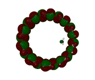
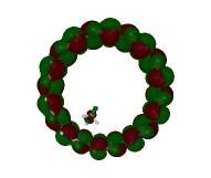
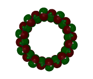
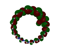
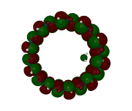
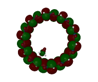
Figure 3: HOMO (top row) and LUMO (bottom row) for the BNNB and the best ranked complexes. Red (green) color represents negative (positive) values. Orbital surfaces were rendered with an isovalue equal to 0.001 and with Jmol software [48] using the CPK color scheme for atoms.

The BNNB, due to its symmetry, presents a homogeneous molecular orbital’s distribution. Depending on the strength of the interaction with the gases, this distribution can be modified. The strongest interaction between NO and BNNB is reflected in the redistribution of the belt wave-functions, concentrated now around the region of interaction with the NO gas. In this case, the DIPRO methodology detected only one fragment, indicating covalent bond formation between BNNB and NO. This is confirmed by the topological results presented in Section 3.3.

The other two gases, NH₃ and CH₃OH, even when bound to the BNNB, induce slight modifications in the orbital surface distribution. In the case of BNNB+NH₃, the calculated values of the effective electron transfer integral are very similar, which is in accordance with the small orbitals’ surface redistribution for both orbitals, HOMO and LUMO. The system BNNB+CH₃OH also shows small surface modifications, but, in accordance with the values of the effective electron transfer integral, the LUMO surfaces experiment with a slightly higher charge redistribution, which is reflected on the BNNB and CH₃OH LUMO surfaces.

MBNNB	MBNNB+NO	MBNNB+NH3	MBNNB+COCl2

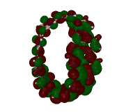
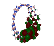
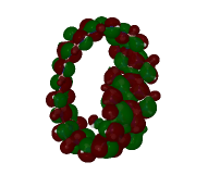
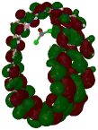
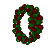
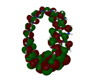
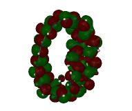
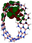
Figure 4: HOMO (top row) and LUMO (bottom row) for the MBNNB and the best ranked complexes. Red (green) color represents negative (positive) values. Orbital surfaces were rendered with an isovalue equal to 0.001 and with Jmol software [48] using the CPK color scheme for atoms.

The Möbius nanobelt, due to the induced twist, broke the frontier orbital distribution. In this case, there is a greater density around the twisted region, and the HOMO is more affected than the LUMO. The high interaction of MBNNB with NO is reflected in the HOMO/LUMO redistribution, localized around the NO adsorption region similar to the BNNB system. In this case, the DIPRO methodology detected the system as having only one fragment, i.e., covalently bonded.

The NH₃ bound to the MBNNB produces a small redistribution of the frontier orbital surfaces, which is in accordance with the similar values for the effective electron transfer integral. On the other hand, even when the interaction of COCl₂ with the MBNNB induced small modifications on the HOMO distribution, the LUMO surface was highly modified, with the surface redistributed around the COCl₂ adsorption region. The latter is reflected in the value of the $J_{un}$ (related to LUMO) that is more than 5 times greater than the value of the $J_{oc}$ (related to HOMO). The types of interactions between MBNNB and COCl₂ are discussed in Section 3.3.

3.3 Topological analysis

The aim of topological analysis is to detect critical points, which are positions where the gradient norm of the electron density value equals zero. The critical points are categorized into four types based on the negative eigenvalues of the Hessian matrix of the real function [50]. The criteria for bond classification and types of critical points are described in detail in ref. [51].

The use of the electron density ($\rho$), Laplacian of the electron density ($\nabla^{2}\rho$), electron localization function (ELF) index, and localized orbital locator (LOL) index, provides insight into the bond type (covalent or non-covalent) in various systems. The localization of electron movement is related to the ELF index, which ranges from 0 to 1 [52; 53]. High values of the ELF index indicate a high degree of electron localization, which suggests the presence of a covalent bond. The LOL index is another function that can be used to identify regions of high localization [54]. The LOL index also ranges from 0 to 1, with smaller (larger) values usually occurring in the boundary (inner) regions.

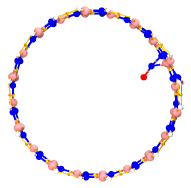
(a) BNNB+NO

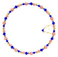
(b) BNNB+NH₃

(c) BNNB+CH₃OH

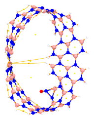
(d) MBNNB+NO

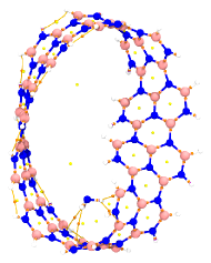
(e) MBNNB+NH₃

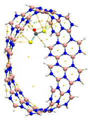
(f) MBNNB+COCl₂

Figure 5: Critical points: BCPs, RCPs and CCPs are represented as orange, yellow, and green dots, respectively. Image rendered with VMD software [55] using the CPK color scheme for atoms.

The calculated critical points for the best ranked complexes are shown in Figure 5. The bond critical points (BCPs) are represented by orange dots, the ring critical points (RCPs) by yellow dots, and the cage critical points (CCPs) by green dots. In the case of BCPs, the calculated descriptor properties are presented in Table 3. Besides the BCPs, RCPs and CCPs are also formed. This implies that the electronic cloud of the belts is modified in a way favorable to the formation of the complexes.

For NO complexes, all the descriptors indicate the formation of two covalent bonds with both types of nanobelts, respectively. In both cases, the nitrogen atom from NO is responsible for interacting with boron, and nitrogen atoms from nanobelts. Higher values for MBNNB+NO’s descriptors imply that the interactions between NO and MBNNB are stronger than with BNNB. This was expected as the adsorption energies are higher for MBNNB+NO than BNNB+NO (see Table 1 and 2). An implication of the interaction between NO and MBNNB is the closing of the Möbius nanobelt and the formation of two new bonds from the atoms in the twisted region with opposite ones (Figure 5(d)). This means that the induced twist created a type of two pockets that gave the Möbius nanobelt more structural flexibility than the non-twisted belt has. This phenomenon was already observed for boron-nitride and carbon-based Möbius nanobelts interacting with metal nanoclusters [56; 57].

The lower values of the descriptors for other complexes (Table 3), suggest that the bonds formed are non-covalent. A close look at figures 5(b), 5(c), 5(e), and 5(f), shows that for the other gases, interactions are mainly with hydrogen and chlorine gas’ atoms. It is well known that hydrogen bond formation is weak and easily breakable compared to covalent bonds [58; 59]. The latter is reflected in the lower recovery times ($\tau$) shown in Tables 1 and 2. A case of interest is the complex MBNNB+COCl₂ where 9 BCPs were found. In one bond, the hydrogen from the nanobelt is involved (BCP no. 301) and in the other five, the chlorine atom from the gas is involved. In this case, even when chlorine has a similar electronegativity to nitrogen (3.16 for Cl and 3.04 for N), the atomic radius of chlorine is higher, causing lower polarization, and, in turn, weaker interactions than nitrogen does.

Table 3: Bond critical points, BCPs, and the atoms involved (nanobelt-gas), $\rho$, $\nabla^{2}\rho$, ELF and LOL descriptors values^†.

System	BCPs (atoms)	$\rho$	$\nabla^{2}\rho$	ELF	LOL
BNNB+NO	310 (N-N)	0.2099	0.0853	0.7300	0.6219
	309 (B-N)	0.1322	0.3923	0.5650	0.5137
BNNB+NH3	286 (N-H)	0.0054	0.0312	0.0074	0.0795
	259 (B-N)	0.0051	0.0260	0.0084	0.0845
BNNB+CH3OH	35 (N-O)	0.0125	0.0607	0.0242	0.1362
	196 (B-H)	0.0033	0.0160	0.0055	0.0697
	214 (N-H)	0.0033	0.0178	0.0048	0.0649
MBNNB+NO	184 (N-N)	0.2371	-0.0092	0.7803	0.6533
	199 (B-N)	0.1337	0.3947	0.5733	0.5176
MBNNB+NH3	191 (N-H)	0.0043	0.0235	0.0065	0.0750
	214 (N-H)	0.0042	0.0243	0.0058	0.0710
	195 (B-H)	0.0040	0.0202	0.0065	0.0748
	175 (N-H)	0.0030	0.0159	0.0043	0.0616
MBNNB+COCl2	284 (N-Cl)	0.0039	0.0287	0.0032	0.0535
	296 (N-Cl)	0.0030	0.0208	0.0026	0.0490
	347 (N-Cl)	0.0030	0.0193	0.0028	0.0508
	337 (N-Cl)	0.0028	0.0205	0.0022	0.0446
	335 (B-Cl)	0.0027	0.0168	0.0025	0.0482
	301 (H-C)	0.0027	0.0145	0.0036	0.0572
	341 (B-O)	0.0020	0.0141	0.0015	0.0369
	323 (N-C)	0.0019	0.0132	0.0014	0.0366
	339 (N-O)	0.0014	0.0105	0.0009	0.0291

^† $\rho$, $\nabla^{2}\rho$, ELF and LOL are in atomic units.

3.4 Molecular dynamics simulation

Molecular dynamics simulations were conducted to elucidate if the interaction between nanobelts and greenhouse gases were stable in time. In case of the BNNB interacting with single molecule gas systems, the complexes BNNB+H₂S, BNNB+CO and BNNB+CH₄ broke apart, with the gas molecule flying away the nanobelt. For CO and CH₄ it is reasonable as they showed low adsorption energies and small recovery times (see Table 1). The adsorption energy of CO₂ is lower than for H₂S but very similar. Therefore, it could be expected that, following the $E_{ads}$ ranking, the CO₂ detached instead H₂S. This behavior could be associated with the difference in mass of those molecules, having H₂S a mass of 34.08 gmol^-1, whereas the mass of CO₂ is higher and equal to 44.01 gmol^-1. For the MBNNB, the complexes MBNNB+H₂S, MBNNB+CO and MBNNB+CH₄ also broke apart following the lowest $E_{ads}$ ranking (see Table 2). The molecular dynamics animations for BNNB interacting with single molecule gas systems can be seen pointing the cell phone camera to the upper QR Code in Figure 6.

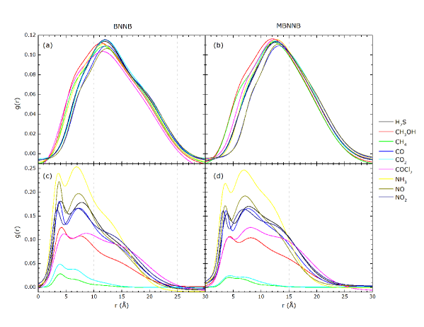
Figure 6: Initial (a,b) and final (c,d) radial distribution functions for all systems calculated with VMD [55] and TRAVIS [60; 61]. Top QR Code: molecular dynamics animations for nanobelts interacting with single gas molecules. Bottom QR Code: molecular dynamics animations for nanobelts interacting with 500 gas molecules.

Figure 6 shows the calculated radial distribution function (RDF) for the packed systems, i.e., nanobelts interacting with 500 gas molecules. Panels 6(a), and 6(b) correspond to the initial complexes as created by PACKMOL software (initial frame). As the molecules are added randomly [46; 47], the RDF shows a Gaussian distribution shape with three visible peaks. Panels 6(c), and 6(d) showed the RDF after 100  ps simulation time. In this case, the three peaks are visible too. All the RDF curves were fitted with three Gaussians, and their peak positions ($r_{1}$, $r_{2}$, and $r_{3}$) are shown in tables 4, and 5 for BNNB and MBNNB, respectively. These peaks represent the shell radii where the particles are found with greater probabilities. In both tables, the top line corresponds to the initial frame ($t=0$ ps) and the bottom line corresponds to the final frame ($t=100$ ps) results.

All the shell radii showed a decrease in value. This means that, at first sight, both nanobelts behave as attractors for all the studied gases. To elucidate this, we determine the number of molecules inside a radius of 10 Å, before ($n_{b}$) and after ($n_{a}$) the simulation, and then the variation, $\Delta n=n_{a}-n_{b}$, is calculated. Positive values of $\Delta n$ indicate that the nanobelts indeed act as attractors for the gas molecules, whereas negative values indicate that the repulsion forces between the gas molecules are greater than the attraction with the nanobelts. Both, CH₄ and CO₂ have shown negative values for $\Delta n$, whereas all other gases have shown positive values. It is worth noting that molecule volume have an important effect here, as molecules like COCl₂ and CH₃OH, well ranked according the adsorption energy (see Tables 1 and 2) present lower positive values $\Delta n$. Finally, the calculation of PMF shows that the free energy change is always favorable, as it is always negative for all the complexes. The molecular dynamics animations for MBNNB interacting with packed molecules gas can be seen by pointing the cell phone camera to the lower QR code in Figure 6.

Table 4: Shells radii, number of molecules inside a shell with 10 Å radius ($n$), percentage of variation on the number of molecules ($\%\Delta n$) in a shell with 10 Å radius after 100 ps MD simulation time, and PMF ($W$) at first shell for BNNB complexes^†.

System	$r_{1}$	$r_{2}$	$r_{3}$	$n$	$\Delta n$	$W(r_{1})$
BNNB+NO	6.938	11.487	18.728	33	—	—
	3.613	6.712	12.163	90	173	-5.679
BNNB+NH3	6.208	10.659	17.457	42	—	—
	3.278	6.253	11.530	115	174	-5.972
BNNB+CH3OH	5.896	10.115	17.073	47	—	—
	3.830	7.004	12.502	50	6	-3.167
BNNB+COCl2	5.795	10.459	16.435	47	—	—
	4.051	7.437	13.862	57	21	-2.758
BNNB+NO2	6.844	11.305	18.670	38	—	—
	3.172	6.298	12.274	77	103	-4.139
BNNB+H2S	6.717	11.225	18.650	38	—	—
	3.698	7.124	12.781	85	124	-4.532
BNNB+CO2	7.041	11.444	18.497	37	—	—
	3.636	6.183	9.688	15	-59	-1.226
BNNB+CO	7.076	11.525	18.853	34	—	—
	3.614	6.697	6.697	76	124	-4.610
BNNB+CH4	5.968	5.968	17.051	42	—	—
	3.752	6.001	9.870	7	-83	-0.723

^† Radii are in units of Å, and $W$ is in units of $eV$.

Table 5: Shells radii, number of molecules inside a shell with 10 Å radius ($n$), percentage of variation on the number of molecules ($\%\Delta n$) in a shell with 10 Å radius after 100 ps MD simulation time, and PMF ($W$) at first shell for MBNNB complexes^†.

System	$r_{1}$	$r_{2}$	$r_{3}$	$n$	$\Delta n$	$W(r_{1})$
MBNNB+NO	8.018	11.855	17.663	25	—	—
	3.372	6.288	10.950	86	244	-4.356
MBNNB+NH3	7.051	11.287	16.866	35	—	—
	3.229	5.972	10.643	114	226	-5.426
MBNNB+COCl2	6.643	11.169	17.243	39	—	—
	3.736	13.173	6.953	60	54	-2.580
MBNNB+CH3OH	5.807	10.399	15.792	45	—	—
	3.913	7.301	12.793	49	9	-2.664
MBNNB+NO2	6.730	11.191	16.940	35	—	—
	3.059	5.957	11.704	76	117	-4.109
MBNNB+CO2	6.748	10.650	15.966	35	—	—
	3.959	6.581	9.333	9	-74	-0.613
MBNNB+CO	8.008	11.800	17.519	26	—	—
	3.575	6.699	11.796	75	188	-4.125
MBNNB+H2S	6.670	10.940	16.406	35	—	—
	3.620	11.970	6.726	78	123	-3.892
MBNNB+CH4	5.612	10.533	15.836	43	—	—
	3.844	6.129	9.906	7	-84	-0.512

^† Radii are in units of Å, and $W$ is in units of $eV$.

4 Conclusions

We can conclude that the answer to the title question is affirmative based on our findings. We provide evidence that boron-nitride nanobelts exhibit varying degrees of sensitivity and specificity in their response to each of the greenhouse gases on the list, in addition to their capability of capturing them.

The adsorption energy of both nanobelts, as determined through optimized geometry calculations, is found to be negative for all gases. However, it is worth noting that the Möbius boron-nitride nanobelt possesses lower adsorption energies for all gaseous substances. The distinct values of the variations in electrical conductivity enable the identification of the interacting gas using the nanobelts. It is feasible to reuse belts that have been adsorbed with gases, given that the recovery time for the highest recovery time is approximately two hours, whereas the recovery times for the remaining systems are in the seconds or even less.

By combining electronic calculations and topological studies, we are able to clarify the manner in which the BNNB and MBNNB belts interact with the enumerated greenhouse gases. Strong covalent bonds can be formed between the nitrogen gas atom and the nitrogen/boron atoms from the belts in the case of NO gas, due to the interaction with both nanobelts. By forming a bond between atoms in opposite positions (from the twisted region), this interaction is able to close the Möbius nanobelt. Topology studies have identified the formation of ring and cage critical points in addition to bond critical points for all of the top-ranked gases, which indicates that the structure of the electronic belts has been altered. BNNB and MBNNB are subject to non-covalent bonding with the remaining gases.

The stability of every complex was subsequently investigated through the utilization of molecular dynamic simulations. There were two types of MD performed. The initial type of investigation focused on the stability of the belts when employing a single gas atom, while the subsequent type examined the behavior of nanobelts when in contact with 500-gas molecules. The complexes BNNB+H₂S, BNNB+CO, BNNB+CH₄, MBNNB+H₂S, MBNNB+CO and MBNNB+CH₄ disintegrated upon initial examination, with the corresponding gases escaping from the belts. These gases are classified as lower interacting gases. The second variant of MD demonstrated a reduction in the radius of the first shell, suggesting a favorable interaction, despite the fact that the quantity of gas molecules within a sphere of 10 Åradius may decrease in certain instances. The free energy change is consistently negative, which signifies a favorable interaction between the nanobelts and each greenhouse gas.

CRediT authorship contribution statement

C. Aguiar: Investigation, Formal analysis, Writing-original draft, Writing-review & editing. N. Dattani: Investigation, Resources, Formal analysis, Writing-original draft, Writing-review & editing. I. Camps: Conceptualization, Methodology, Software, Formal analysis, Resources, Writing-review & editing, Supervision, Project administration.

Declaration of competing interest

The authors declare that they have no known competing financial interests or personal relationships that could have appeared to influence the work reported in this paper.

Data availability

The raw data required to reproduce these findings are available to download from https://doi.org/10.5281/zenodo.10674174.

Funding

The authors declare that no funds, grants, or other support were received during the preparation of this manuscript.

References

- [1] S. W. Lee, W. Lee, Y. Hong, G. Lee, D. S. Yoon, Recent advances in carbon material-based NO2 gas sensors, Sens. Actuators B Chem. 255 (2018) 1788–1804 (2018). doi:10.1016/j.snb.2017.08.203.
- [2] I. Manisalidis, E. Stavropoulou, A. Stavropoulos, E. Bezirtzoglou, Environmental and health impacts of air pollution: A review, Front. Public Health 8 (2020). doi:10.3389/fpubh.2020.00014.
- [3] C. Noöl, C. Vanroelen, S. Gadeyne, Qualitative research about public health risk perceptions on ambient air pollution. a review study, SSM - Population Health 15 (2021) 100879 (2021). doi:10.1016/j.ssmph.2021.100879.
- [4] N. R. Holt, C. P. Nickson, Severe methanol poisoning with neurological sequelae: implications for diagnosis and management, Intern. Med. J. 48 (2018) 335–339 (2018). doi:10.1111/imj.13725.
- [5] J. Y. Jo, Y. S. Kwon, J. W. Lee, J. S. Park, B. H. Rho, W.-I. Choi, Acute respiratory distress due to methane inhalation, Tuberc. Respir. Dis. 74 (2013) 120 (2013). doi:10.4046/trd.2013.74.3.120.
- [6] J. B. Buboltz, M. Robins, Hyperbaric treatment of carbon monoxide toxicity (2023).
- [7] K. Otterness, C. Ahn, Emergency department management of smoke inhalation injury in adults, Emerg. Med. Pract. 20 (2018) 1–24 (2018).
- [8] R. van der Schrier, M. van Velzen, M. Roozekrans, E. Sarton, E. Olofsen, M. Niesters, C. Smulders, A. Dahan, Carbon dioxide tolerability and toxicity in rat and man: A translational study, Front. Toxicol. 4 (2022). doi:10.3389/ftox.2022.1001709.
- [9] R. Rendell, S. Fairhall, S. Graham, S. Rutter, P. Auton, A. Smith, R. Perrott, B. Jugg, Assessment of N-acetylcysteine as a therapy for phosgene-induced acute lung injury, Toxicol. Lett. 290 (2018) 145–152 (2018). doi:10.1016/j.toxlet.2018.03.025.
- [10] J. Pauluhn, Phosgene inhalation toxicity: Update on mechanisms and mechanism-based treatment strategies, Toxicology 450 (2021) 152682 (2021). doi:10.1016/j.tox.2021.152682.
- [11] P. C. Ng, T. B. Hendry-Hofer, A. E. Witeof, M. Brenner, S. B. Mahon, G. R. Boss, P. Haouzi, V. S. Bebarta, Hydrogen sulfide toxicity: Mechanism of action, clinical presentation, and countermeasure development, J. Med. Toxicol. 15 (2019) 287–294 (2019). doi:10.1007/s13181-019-00710-5.
- [12] R. P. Pangeni, B. Timilsina, P. R. Oli, S. Khadka, P. R. Regmi, A multidisciplinary approach to accidental inhalational ammonia injury: A case report, Annals of Medicine & Surgery 82 (2022) 104741 (2022). doi:10.1016/j.amsu.2022.104741.
- [13] A. Amaducci, J. W. Downs, Nitrogen dioxide toxicity (2023).
- [14] G. Verma, A. Gokarna, H. Kadiri, K. Nomenyo, G. Lerondel, A. Gupta, Multiplexed gas sensor: Fabrication strategies, recent progress, and challenges, ACS Sensors 8 (2023) 3320–3337 (2023). doi:10.1021/acssensors.3c01244.
- [15] H. Nazemi, A. Joseph, J. Park, A. Emadi, Advanced micro- and nano-gas sensor technology: A review, Sensors 19 (2019) 1285 (2019). doi:10.3390/s19061285.
- [16] A. Abooali, F. Safari, Adsorption and optical properties of H2S, CH4, NO, and SO2 gas molecules on arsenene: a DFT study, J. Comput. Electron. 19 (2020) 1373–1379 (2020). doi:10.1007/s10825-020-01565-8.
- [17] M. T. Ahmed, S. Islam, F. Ahmed, Density functional theory study of Mobius boron-carbon-nitride as potential CH4 , H2S, NH3, COCl2 and CH3OH gas sensor, R. Soc. Open Sci. 9 (2022) 220778 (2022). doi:10.1098/rsos.220778.
- [18] M. Calvaresi, F. Zerbetto, Atomistic molecular dynamics simulations reveal insights into adsorption, packing, and fluxes of molecules with carbon nanotubes, J. Mater. Chem. A 2 (2014) 12123–12135 (2014). doi:10.1039/c4ta00662c.
- [19] H. M. Cezar, T. D. Lanna, D. A. Damasceno, A. Kirch, C. R. Miranda, Revisiting greenhouse gases adsorption in carbon nanostructures: advances through a combined first-principles and molecular simulation approach, arXiv (2023). doi:10.48550/arXiv.2307.11710.
- [20] C.-C. Chang, I.-K. Hsu, M. Aykol, W.-H. Hung, C.-C. Chen, S. B. Cronin, A new lower limit for the ultimate breaking strain of carbon nanotubes, ACS Nano 4 (2010) 5095–5100 (2010). doi:10.1021/nn100946q.
- [21] J. K. Holt, H. G. Park, Y. Wang, M. Stadermann, A. B. Artyukhin, C. P. Grigoropoulos, A. Noy, O. Bakajin, Fast mass transport through sub-2-nanometer carbon nanotubes, Science 312 (2006) 1034–1037 (2006). doi:10.1126/science.1126298.
- [22] F. Safari, M. Moradinasab, M. Fathipour, H. Kosina, Adsorption of the NH3, NO, NO2, CO2, and CO gas molecules on blue phosphorene: A first-principles study, Appl. Surf. Sci. 464 (2019) 153–161 (2019). doi:10.1016/j.apsusc.2018.09.048.
- [23] X. Tang, M. Debliquy, D. Lahem, Y. Yan, J.-P. Raskin, A review on functionalized graphene sensors for detection of ammonia, Sensors 21 (2021) 1443 (2021). doi:10.3390/s21041443.
- [24] P. Wu, Z. Zhao, Z. Huang, M. Huang, Toxic gas sensing performance of arsenene functionalized by single atoms (Ag, Au): a DFT study, RSC Advances 14 (2024) 1445–1458 (2024). doi:10.1039/d3ra07816g.
- [25] R. B. de Oliveira, D. D. Borges, L. D. Machado, Mechanical and gas adsorption properties of graphene and graphynes under biaxial strain, Sci. Rep. 12 (2022) 22393 (2022). doi:10.1038/s41598-022-27069-y.
- [26] C. Li, Y. Chen, Z. Xu, X. Yang, Quantum mechanical analysis of adsorption for CH4 and CO2 onto graphene oxides, Mater. Chem. Phys. 301 (2023) 127602 (2023). doi:10.1016/j.matchemphys.2023.127602.
- [27] Y. R. Poudel, W. Li, Synthesis, properties, and applications of carbon nanotubes filled with foreign materials: A review, Mater. Today Phys. 7 (2018) 7–34 (2018). doi:10.1016/j.mtphys.2018.10.002.
- [28] A. Alexiadis, S. Kassinos, Molecular dynamic simulations of carbon nanotubes in CO2 atmosphere, Chem. Phys. Lett. 460 (2008) 512–516 (2008). doi:10.1016/j.cplett.2008.06.050.
- [29] G. P. Lithoxoos, A. Labropoulos, L. D. Peristeras, N. Kanellopoulos, J. Samios, I. G. Economou, Adsorption of N2, CH4, CO and CO2 gases in single walled carbon nanotubes: A combined experimental and Monte Carlo molecular simulation study, J. of Supercritical Fluids 55 (2010) 510–523 (2010). doi:10.1016/j.supflu.2010.09.017.
- [30] A. C. Dillon, K. M. Jones, T. A. Bekkedahl, C. H. Kiang, D. S. Bethune, M. J. Heben, Storage of hydrogen in single-walled carbon nanotubes, Nature 386 (1997) 377–379 (1997). doi:10.1038/386377a0.
- [31] J. Lyu, V. Kudiiarov, A. Lider, An overview of the recent progress in modifications of carbon nanotubes for hydrogen adsorption, Nanomaterials 10 (2020) 255 (2020). doi:10.3390/nano10020255.
- [32] M. D. Ganji, M. Asghary, A. A. Najafi, Interaction of methane with single-walled carbon nanotubes: Role of defects, curvature and nanotubes type, Commun. Theor. Phys. 53 (2010) 987–993 (2010). doi:10.1088/0253-6102/53/5/37.
- [33] C. Lu, P. Chen, C. Li, J. Wang, Study of intermolecular interaction between small molecules and carbon nanobelt: Electrostatic, exchange, dispersive and inductive forces, Catalysts 12 (2022) 561 (2022). doi:10.3390/catal12050561.
- [34] Virtual NanoLab - Atomistix ToolKit. QuantumWise. v2017.1 (2017).
- [35] S. Grimme, C. Bannwarth, P. Shushkov, A robust and accurate tight-binding quantum chemical method for structures, vibrational frequencies, and noncovalent interactions of large molecular systems parametrized for all spd-block elements (Z=1–86), J. Chem. Theory Comput. 13 (2017) 1989–2009 (2017). doi:10.1021/acs.jctc.7b00118.
- [36] P. Pracht, E. Caldeweyher, S. Ehlert, S. Grimme, A robust non-self-consistent tight-binding quantum chemistry method for large molecules, ChemRxiv (2019) chemrxiv.8326202.v1 (2019). doi:10.26434/chemrxiv.8326202.v1.
- [37] C. Bannwarth, S. Ehlert, S. Grimme, GFN2–xTB–An accurate and broadly parametrized self-consistent tight-binding quantum chemical method with multipole electrostatics and density-dependent dispersion contributions, J. Chem. Theory Comput. 15 (2019) 1652–1671 (2019). doi:10.1021/acs.jctc.8b01176.
- [38] C. Bannwarth, E. Caldeweyher, S. Ehlert, A. Hansen, P. Pracht, J. Seibert, S. Spicher, S. Grimme, Extended tight-binding quantum chemistry methods, WIREs Comput. Mol. Sci. 11 (2020) e1493 (2020). doi:10.1002/wcms.1493.
- [39] C. Plett, S. Grimme, Automated and efficient generation of general molecular aggregate structures, Angew. Chem. Int. Ed. 62 (2022). doi:10.1002/anie.202214477.
- [40] S. Grimme, C. Bannwarth, E. Caldeweyher, J. Pisarek, A. Hansen, A general intermolecular force field based on tight-binding quantum chemical calculations, J. Chem. Phys. 147 (2017) 161708 (2017). doi:10.1063/1.4991798.
- [41] S. Abdalkareem Jasim, A. H. Shather, T. Alawsi, A. Alexis Ramírez-Coronel, A. B. Mahdi, M. Normatov, M. Jade Catalan Opulencia, F. Kamali, Adsorption properties of B12N12, AlB11N12, and GaB11N12 nanostructure in gas and solvent phase for phenytoin detecting: A DFT study, Inorg. Chem. Commun. 146 (2022) 110158 (2022). doi:10.1016/j.inoche.2022.110158.
- [42] N. Goel, K. Kunal, A. Kushwaha, M. Kumar, Metal oxide semiconductors for gas sensing, Engineering Reports 5 (2023). doi:10.1002/eng2.12604.
- [43] C. Kittel, Introduction to solid state physics, 7th Edition, John Wiley & Sons, Inc., 1996 (1996).
- [44] J. T. Kohn, N. Gildemeister, S. Grimme, D. Fazzi, A. Hansen, Efficient calculation of electronic coupling integrals with the dimer projection method via a density matrix tight-binding potential, J. Chem. Phys. 159 (2023) 144106 (2023). doi:10.1063/5.0167484.
- [45] T. Lu, F. Chen, Multiwfn: A multifunctional wavefunction analyzer, J. Comput. Chem. 33 (2012) 580–592 (2012). doi:10.1002/jcc.22885.
- [46] J. M. Martínez, L. Martínez, Packing optimization for automated generation of complex system's initial configurations for molecular dynamics and docking, J. Comput. Chem. 24 (2003) 819–825 (2003). doi:10.1002/jcc.10216.
- [47] L. Martínez, R. Andrade, E. G. Birgin, J. M. Martínez, PACKMOL: A package for building initial configurations for molecular dynamics simulations, J. Comput. Chem. 30 (2009) 2157–2164 (2009). doi:10.1002/jcc.21224.
- [48] Jmol: An open-source Java viewer for chemical structures in 3D. http://www.jmol.org/.
- [49] J. P. Hansen, I. R. McDonald, Theory of simple liquids, 3rd Edition, Elsevier Science & Technology, London, 2006, description based on publisher supplied metadata and other sources. (2006).
- [50] R. F. W. Bader, Atoms in molecules: a quantum theory, International series of monographs on chemistry, Clarendon Press, Oxford, 1994 (1994).
- [51] I. Camps, Methods used in nanostructure modeling (2023). doi:10.48550/arXiv.2303.01226.
- [52] A. D. Becke, K. E. Edgecombe, A simple measure of electron localization in atomic and molecular systems, J. Chem. Phys. 92 (1990) 5397–5403 (1990). doi:10.1063/1.458517.
- [53] K. Koumpouras, J. A. Larsson, Distinguishing between chemical bonding and physical binding using electron localization function (ELF), J. Phys.: Condens. Matter 32 (2020) 315502 (2020). doi:10.1088/1361-648X/ab7fd8.
- [54] H. L. Schmider, A. D. Becke, Chemical content of the kinetic energy density, J. Mol. Struct.: THEOCHEM 527 (2000) 51–61 (2000). doi:10.1016/S0166-1280(00)00477-2.
- [55] W. Humphrey, A. Dalke, K. Schulten, VMD: Visual molecular dynamics, Journal of Molecular Graphics 14 (1996) 33–38 (1996). doi:10.1016/0263-7855(96)00018-5.
- [56] C. Aguiar, N. Dattani, I. Camps, Möbius boron-nitride nanobelts interacting with heavy metal nanoclusters, Phys. B Condens. Matter 668 (2023) 415178 (2023). doi:10.1016/j.physb.2023.415178.
- [57] C. Aguiar, N. Dattani, I. Camps, Möbius carbon nanobelts interacting with heavy metal nanoclusters, J. Mol. Model. 29 (2023) 277 (2023). doi:10.1007/s00894-023-05669-3.
- [58] G. A. Jeffrey, An introduction to hydrogen bonding, Topics in Physical Chemistry, Oxford University Press, 1997 (1997).
- [59] G. R. Desiraju, T. Steiner, The weak hydrogen bond in structural chemistry and biology, Oxford Science Publications, 1999 (1999).
- [60] M. Brehm, B. Kirchner, TRAVIS - A free analyzer and visualizer for Monte Carlo and molecular dynamics trajectories, J. Chem. Inf. Model. 51 (2011) 2007–2023 (2011). doi:10.1021/ci200217w.
- [61] M. Brehm, M. Thomas, S. Gehrke, B. Kirchner, TRAVIS-A free analyzer for trajectories from molecular simulation, J. Chem. Phys. 152 (2020). doi:10.1063/5.0005078.