How Does Selection Leak Privacy: Revisiting Private Selection and Improved Results for Hyper-parameter Tuning

Abstract.

We study the problem of guaranteeing Differential Privacy (DP) in hyper-parameter tuning, a crucial process in machine learning involving the selection of the best run from several. Unlike many private algorithms, including the prevalent DP-SGD, the privacy implications of tuning remain insufficiently understood. Recent works propose a generic private solution for the tuning process, yet a fundamental question still persists: is the current privacy bound for this solution tight?

This paper contributes both positive and negative answers to this question. Initially, we provide studies affirming the current privacy analysis is indeed tight in a general sense. However, when we specifically study the hyper-parameter tuning problem, such tightness no longer holds. This is first demonstrated by applying privacy audit on the tuning process. Our findings underscore a substantial gap between the current theoretical privacy bound and the empirical bound derived even under the strongest audit setup.

The gap found is not a fluke. Our subsequent study provides an improved privacy result for private hyper-parameter tuning due to its distinct properties. Our privacy results are also more generalizable compared to prior analyses that are only easily applicable in specific setups.

1. Introduction

Differential Privacy (DP) (DBLP:conf/tcc/DworkMNS06, ) stands as the prevailing standard for ensuring privacy in contemporary machine learning. A ubiquitous technique employed to ensure DP across a diverse array of machine learning tasks is differentially private stochastic gradient descent (DP-SGD, a.k.a., noisy-SGD) (bassily2014private, ; song2013stochastic, ; abadi2016deep, ). The ongoing refinement of DP-SGD’s privacy analysis (abadi2016deep, ; balle2018privacy, ; mironov2017renyi, ; rdp_subgaussian_mir, ), referred to as ”privacy accounting” or ”privacy budgeting,” has contributed to a profound comprehension of the mechanism, culminating in the achievement of a tight privacy analysis (nasr2021adversary, ).

In addition to a single (private) training process, machine learning systems always involve a hyper-parameter tuning process that entails running a (private) base algorithm (e.g. DP-SGD) multiple times with different configurations and selecting the best according to some score function. Regrettably, the reasoning for the privacy cost of such tuning operations is inadequately studied and often totally ignored. This is in contrast to extensive studies on the privacy of the base algorithm, as outlined above.

Naively, one can bound the privacy loss for the tuning operation by the composition theorem. If we run the private base algorithm $k$ times with different hyper-parameters, the total privacy cost deteriorates at most linearly with $k$ (or at $\mathcal{O}(\sqrt{k})$ if the base algorithm satisfies approximate DP and we use advanced composition theorem (dwork2014algorithmic, )). However, these bounds are still far from satisfactory as $k$ is usually large in practice. In fact, such bound are generally un-improvable for any fixed $k$ (liu2019private, ; papernot2021hyperparameter, ). Perhaps due to this limitation, it still remains common to exhaustively tune a private algorithm to achieve strong performance but only consider the privacy cost for a single run (de2022unlocking, ; xiao2023theory, ; xiang2023practical, ; shen2023differentially, ).

In essence, private hyper-parameter tuning is closely linked to the private selection problem. Thus, several well-explored mechanisms, such as the sparse vector technique (dwork2009complexity, ) and the exponential mechanism (mcsherry2007mechanism, ), may potentially be utilized. However, these mechanisms presuppose low sensitivity in the score function defining the ”best” to be selected, a condition not always met. Thanks to the contributions of Liu et al. (liu2019private, ) and Steinke et al. (papernot2021hyperparameter, ), hyper-parameter tuning now enjoys significantly better privacy bound than naively applying composition theorem if we do it right. To briefly describe their findings, if we run a private base algorithm a random number of times (possibly with different hyper-parameters) and only output the best single run, the privacy cost only deteriorates by a constant multiplicative factor (liu2019private, ). For example, if the base algorithm is $(\varepsilon,0)$-DP, then the whole tuning process is $(3\varepsilon,0)$-DP if the running number follows a geometric distribution (liu2019private, ). This is much better than the $(k\varepsilon,0)$-DP bound under fixed $k$ times of running. See Section 3.1 for more details.

Steinke et al. (papernot2021hyperparameter, ) improve the analysis within Rényi DP framework by mandating the randomization of the number of running times, presenting additional results for varying degrees of randomness. A noteworthy aspect of both methodologies (liu2019private, ; papernot2021hyperparameter, ) lies in their treatment of the base algorithm as a black box, thus, such a generic approach applies to a broader spectrum of private selection problems, provided the base algorithm is DP on its own.

Motivations. While recent work has facilitated hyper-parameter tuning with a formal privacy guarantee, there remains uncertainty regarding the tightness of the enhanced privacy analysis presented in (papernot2021hyperparameter, ). This concern is due to our ongoing quest for a more precise privacy-utility trade-off. We note that results provided by (liu2019private, ) and (papernot2021hyperparameter, ) show that the privacy cost still increases substantially (e.g., tripling as shown above); however, it also seems plausible that revealing only the best single run should not consume that much privacy budget. This prompts a natural question: Does hyper-parameter tuning truly consume a noticeably larger privacy budget than the base algorithm, as indicated, for instance, by a factor of roughly three in (liu2019private, )?

It is worthwhile to investigate such a problem. A negative answer would imply that a more nuanced privacy-utility trade-off can be achieved through analysis alone, potentially suggesting avenues for improvement. Conversely, a positive answer would indicate limited room for analysis improvement; moreover, it can pinpoint scenarios where privacy is most compromised and provide guidelines for privacy attacks. Importantly, in contrast to the well-established understanding of privacy deterioration due to composition, investigating such a problem contributes to a deeper comprehension of how privacy degrades due to an alternative factor: selection.

Our contributions. In this study, we answer the posed question with both positive and negative answers. In the affirmative, our constructed example demonstrates that the current generic privacy bound provided in (papernot2021hyperparameter, ) for private selection is indeed tight; however, such truth only holds in the worst case. Conversely, in the negative, we uncover a more favorable privacy bound when we consider the hyper-parameter tuning problem, i.e., the base algorithm is the DP-SGD protocol. Our contributions are as follows.

1) Validating tightness of generic privacy bound for private selection. We provide a private selection instance where we observe only a negligible gap between the true privacy cost and the cost predicted by the current privacy bound (papernot2021hyperparameter, ). However, when we open the black box and specifically study the hyper-parameter tuning problem, such tightness no longer holds. This claim is related to our other two contributions.

2) Empirical investigation on the privacy leakage of hyper-parameter tuning. We first take empirical approaches to investigate how much privacy is leaked when adopting the generic approach proposed by Steinke et al. (papernot2021hyperparameter, ) for hyper-parameter tuning. The tool we leverage is the privacy audit technique, which is an interactive protocol used to measure privacy where the adversary makes binary guesses based on the output of a private algorithm. However, different from all previous privacy auditing work, which targets the base algorithm (e.g., DP-SGD), auditing the tuning procedure requires new formulation and insight. Specifically, the score function by which to select the “best” is the new factor that needs to be considered.

We formulate various privacy threat models tailored for hyper-parameter tuning, where the weakest corresponds to the most practical and the strongest corresponds to the worst-case threat. For the weakest, it provides evidence that the tuning process hardly incurs additional privacy costs beyond the base algorithm under the most practical setting. For the strongest, we observe and confirm noticeable additional privacy costs incurred by tuning. However, even the empirical privacy bound derived from the strongest adversary still exhibits a substantial gap from the generic privacy bound proposed by (papernot2021hyperparameter, ), indicating its tightness does not apply to hyper-parameter tuning.

3) Improved privacy results for hyper-parameter tuning. The gap observed in our empirical study is not a fluke. In fact, tuning a DP-SGD protocol does enjoy a better privacy result, as demonstrated by our subsequent study on deriving an improved privacy result for private hyper-parameter tuning.

Our strategy involves first instantiating the strongest hypothetical adversary and then employing divergence-based analytical approaches. Note that the private tuning problem introduces an additional factor: the score function, which serves as the metric for selecting the best-trained model. We prove that considering only a specific family of score functions is sufficient to analyze the privacy cost. We show that our results surpass the previous generic bound under various settings; particularly, under the same settings, the tuning procedure only incurs limited additional privacy costs, much better than what’s predicted by previous work (liu2019private, ; papernot2021hyperparameter, ). We also validate our approach through privacy audit experiments, demonstrating it is nearly tight, i.e., there is only a negligible gap between the empirical privacy bound and our improved bound. In addition, our results are more generalizable, contrasting to previous work where they only easily apply in specific setups. To give a concise summary of our main contributions:

• We confirm the general tightness of the current generic privacy bound for private selection.

• We conduct comprehensive experiments evaluating privacy leakage for the current private hyper-parameter tuning protocol under various privacy threat models.

• For private hyper-parameter tuning, we provide improved privacy results, which are shown to be nearly tight.

2. Background

2.1. Differential Privacy (DP)

Definition 0.

(Differential Privacy (DBLP:conf/tcc/DworkMNS06, )) Given a data universe $\mathcal{X}$, two datasets $X,X^{\prime}\subseteq\mathcal{X}$ are adjacent if they differ by one data example. A randomized algorithm $\mathcal{M}$ is $(\varepsilon,\delta)$-differentially private if for all adjacent datasets $X,\,X^{\prime}$ and for all events $S$ in the output space of $\mathcal{M}$, we have $\operatorname{Pr}(\mathcal{M}(X)\in S)\leq e^{\varepsilon}\operatorname{Pr}(\mathcal{M}(X^{\prime})\in S)+\delta$.

Randomness by Differential Privacy (DP) conceals evidence of participation by weakening the causal effect from the differing data point to the output (DBLP:conf/sp/TschantzSD20, ). DP is resilient to post-processing, and the execution of multiple DP algorithms sequentially, known as composition, also maintains DP. For algorithms having compositions, Rényi Differential Privacy (RDP) often serves as an analytical tool to assess the overall privacy cost while giving tight results.

Definition 0 (Rényi DP (RDP) (DBLP:conf/csfw/Mironov17, )).

The Rényi divergence is defined as $\mathcal{D}_{\alpha}(M||N)=\frac{1}{\alpha-1}\ln\mathbb{E}_{x\sim N}\left[\frac{M(x)}{N(x)}\right]^{\alpha}$ with $\alpha>1$. A randomized mechanism $\mathcal{M}:\mathcal{X}\rightarrow\mathcal{Y}$ is said to be $(\alpha,\gamma)$-RDP, if $\mathcal{D}_{\alpha}(\mathcal{M}(X)||\mathcal{M}(X^{\prime}))\leq\gamma$ holds for any adjacent dataset $X,X^{\prime}$.

Composition by RDP results in linear add-up in $\gamma$ for the same $\alpha$. Usually, one wants to convert an RDP guarantee to the more interpretable $(\varepsilon,\delta)$-DP formulation. And Theorem 20 in (balle2020hypothesis, ) (shown in Appendix A.2) allows to make such conversion tightly.

Differentially private stochastic gradient descent (DP-SGD) (bassily2014private, ; song2013stochastic, ; abadi2016deep, ). A machine learning model denoted as $f_{w}$ represents a neural network with trainable parameters $w$. Specifically tailored for classification tasks in this study, $f_{w}$ may take image data as input and output corresponding labels. Stochastic Gradient Descent (SGD) (lecun1998gradient, ) serves as the iterative training method for updating $w$. Hyper-parameters, such as the updating step size (a.k.a. learning rate), often require to be tuned to gain optimized performance.

As the private version of SGD, DP-SGD obfuscates the computed gradient as follows. 1) DP-SGD computes the per-sample gradient for each sub-sample data, 2) clips each gradient to have bounded $l_{2}$ norm, and 3) adds Gaussian noise (Gaussian mechanism). The resultant private gradient $p_{i}$ is used to update parameter $w$, and $i$-th (from $1$ to $N$) update from can be expressed as:

(1) $$p_{i}=\sum_{(x,y)\in\mathbf{B}}\operatorname{CLP}_{C}\left(\nabla_{w}\ell\left(w_{i-1};x,y\right)\right)+R_{i}$$

$$w_{i}\leftarrow w_{i-1}-\mathbf{lr}\cdot p_{i}$$

where $\mathbf{lr}$ is the learning rate and data batch $\mathbf{B}$ contains the sub-sampled data where the sample ratio is $\tau$. For instance, $x$ may represent an image, and $y$ is its label. The function $\operatorname{CLP}_{C}(u)=\min(1,\frac{C}{\|u\|_{2}})u$ where the clipping threshold $C$ is a hyper-parameter. $R_{i}$ is calibrated isotropic Gaussian noise sampled from $\mathcal{N}(0,C^{2}\sigma^{2}\mathbb{I}^{d})$ where $d$ is the dimension or number of trainable parameters. $\ell(;)$ is the loss function that represents the neural network $f_{w}$ and some loss metric (e.g. cross-entropy loss). With $R_{i}$ and $\operatorname{CLP}_{C}$ operation eliminated, we recover SGD. The basis for analyzing DP-SGD’s privacy is that we only need to inspect the distribution of $p_{i}$, because any further operation taking $p_{i}$ as input is post-processing. To ensure $(\varepsilon,\delta)$-DP, we can set the above $\sigma$ as

(2) $$\sigma=\Theta(\varepsilon^{-1}\tau\sqrt{N\log\delta^{-1}})$$

as shown by Theorem 1 in (abadi2016deep, ).

2.2. Operational Perspective of DP

Hypothesis testing interpretation of DP. For a randomized mechanism $\mathcal{M}$, let $X,X^{\prime}$ be adjacent datasets, let $y$ be the output of $\mathcal{M}(\hat{X})$, we form the null and alternative hypotheses:

$$\mathbf{H_{0}}:\text{$\hat{X}=X$},\text{\quad}\mathbf{H_{1}}:\text{$\hat{X}=X^{\prime}$}.$$

For a decision rule $\mathcal{R}$ in such a hypothesis testing problem, it has two notable types of errors: 1) type I error $FP$, a.k.a. false positive, the action of rejecting $\mathbf{H_{0}}$ while $\mathbf{H_{0}}$ is true; 2) type II error $FN$ a.k.a. false negative, the action of rejecting $\mathbf{H_{1}}$ while $\mathbf{H_{1}}$ is true. Differential privacy then can be characterized by such two error rates as follows.

Theorem 3 (DP as Hypothesis Testing (kairouz2015composition, )).

For any $\varepsilon>0$ and $\delta\in[0,1]$, a mechanism $\mathcal{M}$ is $(\varepsilon,\delta)$-DP if and only if

(3) $$FP+\mathrm{e}^{\varepsilon}FN\geq 1-\delta,\text{\quad}FN+\mathrm{e}^{\varepsilon}FP\geq 1-\delta$$

both hold for any adjacent dataset $X,X^{\prime}$ and any decision rule $\mathcal{R}$ in a hypothesis testing problem as defined in eq. 9.

Theorem 3 has the following implications. With $\delta$ fixed at some value, under the threat model that an adversary can only operate at some $FP$ and $FN$ rate under some decision rule $\mathcal{R}$ for a specific adjacent dataset pair $X,X^{\prime}$, a lower bound

(4) $$\varepsilon_{L}^{(X,X^{\prime},\mathcal{R})}=\max\{\log\frac{1-\delta-FP}{FN},\log\frac{1-\delta-FN}{FP},0\}$$

can be computed, meaning that the algorithm can’t be more private than that, i.e., the true privacy parameter $\varepsilon_{T}\geq\varepsilon_{L}^{(X,X^{\prime},\mathcal{R})}$. This forms the basis for the privacy audit technique, as will be shown below. However, if there exists the strongest adversary that can operate for every adjacent pair $X,X^{\prime}$ at every $FP$ rate and can carry out the most powerful test (achieving lowest $FN$ rate) enabled by Neyman-Pearson lemma (neyman1933ix, ), we then can get the true value for the privacy parameter

(5) $$\varepsilon_{T}=\max_{X,X^{\prime}}\max_{\mathcal{R}}\varepsilon_{L}^{(X,X^{\prime},\mathcal{R})},$$

just as entailed by theorem 3. However, using eq. 5 to find $\varepsilon_{T}$ is clearly intractable generally. In practice, a upper bound $\varepsilon_{U}\geq\varepsilon_{T}$ is obtained as the privacy claim by analytical approaches (e.g., privacy accounting using RDP) (abadi2016deep, ; mironov2017renyi, ; rdp_subgaussian_mir, ). It means that the algorithm is at least as private as $\varepsilon_{U}$ claims for some fixed $\delta$.

Algorithm 1 Game-based Privacy Audit $\mathcal{G}$

1:DP protocol $\mathcal{P}$, adjacent pair $X,X^{\prime}$

2:$b_{truth}\leftarrow\{0,1\}$ $\triangleright$ Trainer flips a fair coin

3:$\hat{X}\leftarrow X$ if $b_{truth}=0$, $\hat{X}\leftarrow X^{\prime}$ otherwise

4:Run $\mathcal{P}(\hat{X})$ $\triangleright$ Trainer runs the private protocol

5:$b_{guess}\leftarrow\{0,1\}$ $\triangleright$ Adversary makes a guess based on $\mathcal{P}(\hat{X})$

6:$(b_{truth},b_{guess})$

Privacy audit. Privacy audit is an empirical approach that finds a lower bound of the privacy cost for a private protocol $\mathcal{P}$. This is done by simulating the interactive game-based protocol described in Algorithm 1. Such a simulation is typically repeated many times, which gives many pairs of $(b_{truth},b_{guess})$. Then, the $FP$ and $FN$ rates for adversary’s guessing are computed by Clopper-Pearson method (clopper1934use, ), which means that lower bound $\varepsilon_{L}^{(X,X^{\prime},\mathcal{R})}$ computed by eq. 4 is with a confidence specification.

A lower bound $\varepsilon_{L}^{(X,X^{\prime},\mathcal{R})}$ found by the above procedure is useful for assessing the privacy of a mechanism. Intuitively, if the adversary can make accurate guesses, it will indicate the algorithm is not very private. Quantitatively, this is demonstrated by that the adversary attains very low $FN,FP$, which leads to a high value of $\varepsilon_{L}^{(X,X^{\prime},\mathcal{R})}$, suggesting $\varepsilon_{T}$’s value is also high. Note that the weakest lower bound $\varepsilon_{L}^{(X,X^{\prime},\mathcal{R})}=0$ is not informative at all, and stronger (with larger value) $\varepsilon_{L}^{(X,X^{\prime},\mathcal{R})}$ is more favored.

Notably, Nasr et al. (nasr2023tight, ) improved over eq. 4 to find stronger $\varepsilon_{L}^{(X,X^{\prime},\mathcal{R})}$ with less number of simulating the distinguishing game (Algorithm 1). Briefly, the method in (nasr2023tight, ) finds the functional relationship between $FP$ and $FN$ rates and can then derive a range of $(FP,FN)$ pairs based on a single $(FP,FN)$ experimental result. Then, the strongest/largest $\varepsilon_{L}^{(X,X^{\prime},\mathcal{R})}$ value can be computed based on the derived range of $(FP,FN)$ results.

2.3. Problem Formulation

We formulate the private hyper-parameter tuning/private selection problem following (liu2019private, ; papernot2021hyperparameter, ). Let $\Omega=\{\mathcal{M}_{1},\mathcal{M}_{2},\cdots,\mathcal{M}_{m}\}$ be a collection of DP-SGD algorithms. These correspond to $m$ possible hyper-parameter configurations. We have $\mathcal{M}_{i}:\mathcal{X}\rightarrow\mathcal{Y}$ for $i\in[m]$, and all of these algorithms satisfy the same privacy parameter, i.e., they are all $(\varepsilon,\delta)$-DP for some $\varepsilon,\delta$. The practitioner can freely determine the size of $\Omega$.

The goal is to return an algorithm element (including its execution) of $\Omega$ such that the output of such algorithm has (approximately) the maximum score as specified by some score function $g:\mathcal{Y}\rightarrow\mathbb{R}$. It is also assumed that there is an arbitrary dataset-independent tie-breaking rule when there are two elements leading to the same score. The score function $g$ usually serves a utility purpose (e.g., $g$ could evaluate the validation loss on a held-out dataset). The selection of that element must be performed in a differentially private manner. The general private selection problem corresponds to the cases where $\Omega$ contains some arbitrary differentially private algorithms processing the same privacy parameter.

2.4. Related Work

Privacy audit. In privacy-preserving machine learning, privacy audit mainly serves a different goal from that of certain earlier studies (wang2020checkdp, ; ding2018detecting, ; bichsel2021dp, ; bichsel2018dp, ) on detecting privacy violation in general query-answering applications. Previous work on privacy audit in machine learning mainly targets auditing the DP-SGD protocol to assess its theoretical versus practical privacy (nasr2021adversary, ; kairouz2015composition, ; jagielski2020auditing, ). Additional studies (steinke2023privacy, ; nasr2023tight, ; lu2022general, ; zanella2023bayesian, ) concentrate on enhancing the strength of audits on DP-SGD (yielding stronger/larger $\varepsilon_{L}^{(X,X^{\prime},\mathcal{R})}$) or improving the efficiency (incurring fewer simulation overheads). Drawing a parallel to the action of guessing whether a data point was included or not, privacy audit may also be linked to a topic called membership inference attack (hayes2017logan, ; nasr2019comprehensive, ; shokri2017membership, ), which sees a notable work by Shokri et al. (shokri2017membership, ). However, privacy audits diverge from membership inference attacks in terms of both their goals and methodologies.

Private selection and private hyper-parameter tuning. Well-established algorithms like the sparse vector technique (dwork2009complexity, ) and exponential mechanism (mcsherry2007mechanism, ) may potentially be leveraged to the privacy hyper-parameter tuning problem; however, they assume a low sensitivity in the metric defining the ”best,” a condition not always applicable. Some earlier work (chaudhuri2013stability, ) also suffers from the same issue. Steinke et al. (papernot2021hyperparameter, ) and Liu (liu2019private, ) have provided generic private selection approaches circumventing such challenges. Mohapatra et al. (mohapatra2022role, ) study privacy issues in adaptive hyper-parameter tuning under DP, which is different from the non-adaptive tuning problem considered in this work. There is related work (koskela2023practical, ) that builds upon (papernot2021hyperparameter, ); therefore, what we understand about the generic approach in this study also applies to (koskela2023practical, ).

This work. In essence, existing works on privacy audit in learning tasks examine the practical versus theoretical privacy under composition. Our first focus is on understanding how privacy deteriorates for a distinct reason: selection. Furthermore, we also study improving privacy results specifically for a white-box application: the hyper-parameter tuning problem, where the base algorithm is DP-SGD.

Algorithm 2 Private Hyper-parameter Tuning $\mathcal{H}$

1:Dataset $X$; algorithms $\Omega$; distribution $\xi$; score function $g$

2:Draw a sample: $k\leftarrow\xi$

3:$Y\leftarrow\text{{Null}}$, $S\leftarrow-\infty$

4:for $i=1,2,\cdots,k$ do

5:     Randomly fetch one element $\mathcal{M}_{i}$ from $\Omega$ in uniform

6:     $y_{i}\leftarrow\mathcal{M}_{i}(X)$ $\triangleright$ Run $\mathcal{M}_{i}$

7:     If $g(y_{i})>S$: $Y\leftarrow y_{i}$, $S\leftarrow g(y_{i})$ $\triangleright$ Selecting the “best”

8:end for

9:$Y$

3. The Private Selection Protocol

3.1. Private Hyper-parameter Tuning

The state-of-the-art private algorithm (liu2019private, ; papernot2021hyperparameter, ) for hyper-parameter tuning is outlined in Algorithm 2. Notably, this generic algorithm is also adaptable to other applications as long as the base algorithm is private on its own. A noteworthy point of Algorithm 2 is that the base algorithm is repeated by a random number of times (according to distribution $\xi$) instead of a fixed number of times.

Current privacy analysis. Specifically, if the base DP algorithm $\mathcal{M}$ is $(\varepsilon,0)$-DP (pure DP) and $\xi$ is a geometric distribution, Algorithm 2 is $(3\varepsilon,0)$-DP (liu2019private, ). An improved bound for the pure DP case is provided in (papernot2021hyperparameter, ) by replacing the distribution $\xi$ with the Truncated Negative Binomial (TNB) distribution at some specific parameter setups, as shown in Appendix A.1. This improvement is achieved through RDP analysis. In addition to the RDP results when $\xi$ is from the TNB family, (papernot2021hyperparameter, ) also provides RDP results when $\xi$ follows a Poisson distribution.

3.2. Current Generic Privacy Bound is Tight

Our discussion in this section shows that the current privacy bound due to (papernot2021hyperparameter, ) is tight in a general sense. It suffices to provide some instances of the tuple $(\Omega,\xi,g)$ observing such tightness.

Example 0 (Pure DP Case).

Suppose $\mathcal{M}$ has a finite output space $\mathcal{Y}=\{\mathrm{A},\mathrm{B},\mathrm{C}\}$, and let $\operatorname{Pr}_{\mathcal{M}},\operatorname{Pr}_{\mathcal{M^{\prime}}}$ denote the probabilities for each event when $\mathcal{M}$ operates on two adjacent dataset $X,X^{\prime}$, which gives

(6) $$\operatorname{Pr}_{\mathcal{M}}:\left\{\begin{array}[]{ll}\operatorname{Pr}_{\mathrm{A}|\mathcal{M}}=1-b\mathrm{e}^{\varepsilon}-db\\ \operatorname{Pr}_{\mathrm{B}|\mathcal{M}}=b\mathrm{e}^{\varepsilon}\\ \operatorname{Pr}_{\mathrm{C}|\mathcal{M}}=db\\ \end{array}\right.\operatorname{Pr}_{\mathcal{M^{\prime}}}:\left\{\begin{array}[]{ll}\operatorname{Pr}_{\mathrm{A}|\mathcal{M}^{\prime}}=1-b-db\mathrm{e}^{\varepsilon}\\ \operatorname{Pr}_{\mathrm{B}|\mathcal{M}^{\prime}}=b\\ \operatorname{Pr}_{\mathrm{C}|\mathcal{M}^{\prime}}=db\mathrm{e}^{\varepsilon}\\ \end{array}\right.$$

where $\operatorname{Pr}_{\mathrm{A}|\mathcal{M}}$ denotes the probability of event $A$ occurs conditioned on $\mathcal{M}$ operates on $X$ (similarly we also have $\operatorname{Pr}_{\mathrm{A}|\mathcal{M}^{\prime}}$). With $b=10^{-3},d=10^{2},\varepsilon=1$, we can see $\mathcal{M}$ is $(1,0)$-DP.

Let each element of $\mathcal{M}_{i}$ fetched from $\Omega$ in line 5 of Algorithm 2 has the same output distribution as eq. 6. Also let a score function $g$ give $g(\mathrm{C})>g(\mathrm{B})>g(\mathrm{A})$. Let $\xi$ be the TNB distribution with parameter $\eta=1,\nu=10^{-3}$ (geometric distribution). The probability for each event that Algorithm 2 outputs is computed by the following theorem.

Theorem 2.

Let $y$ be some event in $\mathcal{Y}$, the probability of $y$ occurs as the output of the tuning process $\mathcal{H}$ (Algorithm 2) is

(7) $$\operatorname{Pr}(y)=\sum_{k\sim\xi}\operatorname{Pr}(k)\left(\operatorname{Pr}(E_{\leq y})^{k}-\operatorname{Pr}(E_{<y})^{k}\right),$$

where $E_{\leq y}=\{x:g(x)\leq g(y)\}$ and $E_{<y}=\{x:g(x)<g(y)\}$.

Let $\operatorname{Pr}_{\mathcal{H}},\operatorname{Pr}_{\mathcal{H^{\prime}}}$ denote the probabilities for each event conditioned on $\mathcal{H}$ operates on $X,X^{\prime}$, respectively. For $\operatorname{Pr}_{\mathcal{H}}$ we have

$$\operatorname{Pr}_{\mathcal{H}}:\left\{\begin{array}[]{ll}\operatorname{Pr}_{\mathrm{A}|\mathcal{H}}=\sum_{k\sim\xi}\operatorname{Pr}(k)\operatorname{Pr}_{\mathrm{A}|\mathcal{M}}^{k}\\ \operatorname{Pr}_{\mathrm{B}|\mathcal{H}}=\sum_{k\sim\xi}\operatorname{Pr}(k)((\operatorname{Pr}_{\mathrm{A}|\mathcal{M}}+\operatorname{Pr}_{\mathrm{B}|\mathcal{M}})^{k}-\operatorname{Pr}_{\mathrm{A}|\mathcal{M}}^{k})\\ \operatorname{Pr}_{\mathrm{C}|\mathcal{H}}=\sum_{k\sim\xi}\operatorname{Pr}(k)(1-(\operatorname{Pr}_{\mathrm{A}|\mathcal{M}}+\operatorname{Pr}_{\mathrm{B}|\mathcal{M}})^{k})\\ \end{array}\right.$$

$\operatorname{Pr}_{\mathcal{H^{\prime}}}$ can be computed similarly. Numerically, this gives the probabilities shown below

(8) $$\operatorname{Pr}_{\mathcal{H}}:\left\{\begin{array}[]{ll}\operatorname{Pr}_{\mathrm{A}|\mathcal{H}}=8.66\times 10^{-3}\\ \operatorname{Pr}_{\mathrm{B}|\mathcal{H}}=2.60\times 10^{-4}\\ \operatorname{Pr}_{\mathrm{C}|\mathcal{H}}=9.91\times 10^{-1}\\ \end{array}\right.\operatorname{Pr}_{\mathcal{H^{\prime}}}:\left\{\begin{array}[]{ll}\operatorname{Pr}_{\mathrm{A}|\mathcal{H}^{\prime}}=2.66\times 10^{-3}\\ \operatorname{Pr}_{\mathrm{B}|\mathcal{H}^{\prime}}=1.34\times 10^{-5}\\ \operatorname{Pr}_{\mathrm{C}|\mathcal{H}^{\prime}}=9.97\times 10^{-1}\\ \end{array}\right.$$

and it can be checked to satisfy $(2.96,0)$-DP. The theoretical bound claims Algorithm 2 is $(3,0)$-DP, i.e., it is tight up to a negligible gap.

In the same manner, tightness can also be verified under various $(\eta,\nu)$ setups of TNB. For the approximate DP case ($\delta>0$), a tight example can be obtained with a trick trivially and is provided in Appendix A.1. Now we confirm the privacy bound (liu2019private, ; papernot2021hyperparameter, ) for private selection problems is indeed tight. However, the example we provided stands for the worst case. Does this tightness still hold for private hyper-parameter tuning where the selection is among several executions of DP-SGD protocol? This leads to our following investigations.

Notation	Meaning
$\mathcal{G}$	The distinguishing game, Algorithm 1
$\mathcal{P}$	A general protocol to be audited in $\mathcal{G}$
$\mathcal{H}$	The private tuning protocol, Algorithm 2
$\mathcal{M}$	The base algorithm (a DP-SGD instance) of $\mathcal{H}$
$\mathbb{F},\mathbb{M},\mathbb{C},\mathbb{S}$	Datasets used, shown in Table 2
$N$	Number of iterations inside $\mathcal{M}$
$\xi$	Running number distribution inside $\mathcal{H}$
$g$	Score function evaluating $\mathcal{M}$’s output
$\mathbf{z}$	Differing data point, constructed by adversary
$p_{i}^{\mathbf{z}}$	$\mathbf{z}$’s gradient at $i$-th iteration in eq. 1
$\mathbf{Z}_{D}$	Malicious instance of $\mathbf{z}$ leading to Dirac gradient
$p_{i}$	Private gradient in eq. 1
$\lambda_{a},\lambda_{b}$	Two proxies constructed by the adversary for assertion
$\sigma$	Noise s.t.d. for $R_{i}$ in eq. 1
$\varepsilon_{B}$	Base algorithm $\mathcal{M}$’s privacy budget for a single run
$\varepsilon_{L}$	Lower bound for $\mathcal{H}$ by audit
$\varepsilon_{U}$	Generic theoretical upper bound for $\mathcal{H}$, computed by (papernot2021hyperparameter, )

Table 1. Notations used in our empirical study.

4. Empirical Investigation

In this section, we aim to leverage privacy audit techniques to assess the extent of privacy compromise resulting from the tuning procedure $\mathcal{H}$. The high-level procedure is to simulate the distinguishing game $\mathcal{G}$ (Algorithm 1) and then conclude the lower bound. Notations used are summarised in Table 1.

4.1. Deriving the Lower Bound: Procedure

This part is essentially on how we instantiate $\mathcal{G}$ and derive the lower bound $\varepsilon_{L}^{(X,X^{\prime},\mathcal{R})}$. We clarify the terminology and describe the designs/setups for our audit in the following.

Interaction. The trainer plays the role of executing the protocol $\mathcal{P}$ honestly and does not reveal any sensitive information to the adversary other than what the DP protocol allows. The adversary instantiates two input arguments to $\mathcal{G}$: $\mathcal{P}$ and adjacent dataset pair $X,X^{\prime}$. Then, the trainer flips a fair coin and chooses one dataset as $\mathcal{P}$’s input. Finally, the adversary makes assertions/guesses based on $\mathcal{P}$’s output.

$\mathcal{P}$ is the tuning protocol. Note that each execution of $\mathcal{P}$ in $\mathcal{G}$ is a running of our tuning protocol $\mathcal{H}(\mathbf{x},\mathcal{M},\xi,g)$ where $\mathbf{x}$ can be $X$ or $X^{\prime}$, the base algorithm $\mathcal{M}$ is a DP-SGD instance, $\xi$ is the TNB distribution (papernot2021hyperparameter, ) shown in Appendix A.1 with parameter $(\eta=0,\nu=10^{-2})$ and the score function $g$ is the metric defining the best execution. $w$ and $\ell(;)$ are defined as shown in eq. 1.

Forming adjacent dataset pair $X,X^{\prime}$. W.o.l.g., we assume $X^{\prime}=X\cup\mathbf{z}$. Different adjacent pair setup corresponds to different adversary’s power. By design, the adversary needs to make guesses as accurate as possible. This is done by forging appropriate $\mathbf{z}$, then inserting $\mathbf{z}$, and finally trying to recover the trace of $\mathbf{z}$. $\mathbf{z}$ is known in the literature as “canaries”. Since this setup is of no significant difference from previous privacy audit tasks, we consider two different types of adversary following previous work (nasr2023tight, ).

1) input space canary, the adversary can select $\mathbf{z}$ to be any real-world data, and to have higher distinguishing performance, $\mathbf{z}$ is set to be sampled from a distribution different from those in $X$; 2) gradient canary, the adversary can directly control the gradient of $\mathbf{z}$. Specifically, it is assumed that adversary generates $\mathbf{z}=\mathbf{Z}_{D}$ such that its gradient is a Dirac vector $\nabla_{w}\ell(w;\mathbf{Z}_{D})=[C,0,0,\cdots,0]^{T}$ (nasr2023tight, ), i.e., only the first coordinate equals to the clipping threshold $C$ and the rest are all zeros. Note that the first type corresponds to the practical case, whereas the second is for worst-case privacy investigation. Our analysis in Section 5.1 will explain why the Dirac vector suffices to be worse-case.

Observation. The adversary makes assertions based on the observation, which is the output in line 4 of Algorithm 1 or the output of $\mathcal{H}$. Under the assumption of DP-SGD protocol, the whole trajectory of the training is released. This means that $\{p_{1},p_{2},\cdots\,p_{N}\}$ is released. Equivalently, all the checkpoints $\{w_{1},\cdots,w_{N}\}$ of the neural network are also released as each checkpoint is just post-processing of the private gradient. Hence, we can denote the observation as $y=\{p_{1},p_{2},\cdots\,p_{N},w_{1},\cdots,w_{N}\}$.

Score function $g$. W.o.l.g., the best model is selected if it has the highest score. This new factor distinguishes auditing hyper-parameter tuning from all previous auditing tasks. We formalize two types of adversaries that are only possible.

1) The adversary is not able to manipulate $g$, e.g., $g$ is a normal routine to evaluate the model’s accuracy/loss on an untampered validation dataset; 2) the adversary can arbitrarily control $g$, e.g., $g$ can be a routine to evaluate the model’s performance on some malicious dataset. The first type corresponds to more practical and normal cases. The second probably does not exist in real-world applications and is included purely for worst-case privacy investigation. Because manipulating the score function is allowed by the private selection protocol, we can give the adversary such power so that the worst-case condition is explored. Additionally, the adversary also knows the score as it can be trivially computed from the observation by the score function $g$.

Identifier	Adjacent $X,X^{\prime}=X\cup\mathbf{z}$	Score Function $g$		Observation $y$	Audit Results
NTNV	1: $X\leftarrow\mathbb{F},\text{\quad}\mathbf{z}\leftarrow\mathbb{M}[I]$ 2: $X\leftarrow\mathbb{C},\text{\quad}\mathbf{z}\leftarrow\mathbb{S}[I]$ 3: $X\leftarrow\mathbb{S},\text{\quad}\mathbf{z}\leftarrow\mathbb{C}[I]$ 4: $X\leftarrow\mathbb{F},\text{\quad}\mathbf{z}\leftarrow\mathbf{Z}_{D}$ 5: $X\leftarrow\mathbb{C},\text{\quad}\mathbf{z}\leftarrow\mathbf{Z}_{D}$ 6: $X\leftarrow\mathbb{S},\text{\quad}\mathbf{z}\leftarrow\mathbf{Z}_{D}$	1: $g(y)=-\sum_{i}\ell(y[w_{N}];\mathbb{F}_{v}[i])$ 2: $g(y)=-\sum_{i}\ell(y[w_{N}];\mathbb{C}_{v}[i])$ 3: $g(y)=-\sum_{i}\ell(y[w_{N}];\mathbb{S}_{v}[i])$	4: $g(y)=-\sum_{i}\ell(y[w_{N}];\mathbb{F}_{v}[i])$ 5: $g(y)=-\sum_{i}\ell(y[w_{N}];\mathbb{C}_{v}[i])$ 6: $g(y)=-\sum_{i}\ell(y[w_{N}];\mathbb{S}_{v}[i])$	$\{p_{i}\}_{i=1}^{N}\&\{w_{i}\}_{i=1}^{N}$	1: fig. 1(a)  4: fig. 1(d) 2: fig. 1(b)  5: fig. 1(e) 3: fig. 1(c)  6: fig. 1(f)
NTCV		1: $g(y)=-\ell(y[w_{N}];\mathbf{z})$ 2: $g(y)=-\ell(y[w_{N}];\mathbf{z})$ 3: $g(y)=-\ell(y[w_{N}];\mathbf{z})$	4: $g(y)=(y[w_{0}]-y[w_{N}])[0]$ 5: $g(y)=(y[w_{0}]-y[w_{N}])[0]$ 6: $g(y)=(y[w_{0}]-y[w_{N}])[0]$		1: fig. 2(a)  4: fig. 2(d) 2: fig. 2(b)  5: fig. 2(e) 3: fig. 2(c)  6: fig. 2(f)
ETCV	1: $X\leftarrow\emptyset,\text{\quad}\mathbf{z}\leftarrow\mathbb{M}[I]$ 2: $X\leftarrow\emptyset,\text{\quad}\mathbf{z}\leftarrow\mathbb{S}[I]$ 3: $X\leftarrow\emptyset,\text{\quad}\mathbf{z}\leftarrow\mathbb{C}[I]$ 4: $X\leftarrow\emptyset,\text{\quad}\mathbf{z}\leftarrow\mathbf{Z}_{D}$	1: $g(y)=-\ell(y[w_{N}];\mathbf{z})$ 2: $g(y)=-\ell(y[w_{N}];\mathbf{z})$ 3: $g(y)=-\ell(y[w_{N}];\mathbf{z})$	4: $g(y)=(y[w_{0}]-y[w_{N}])[0]$		1: fig. 3(a) 4: fig. 4 2: fig. 3(b) 3: fig. 3(c)

Table 2. Experiment setups of our audit experiments. $\mathbb{F}$ stands for the FASHION dataset, $\mathbb{M}$ for MNIST dataset, $\mathbb{C}$ for CIFAR10 dataset and $\mathbb{S}$ stands for the SVHN dataset. Details for all datasets used are presented in Appendix A.3. We use $\mathbb{F}_{v}$ to stand for the validation dataset counterpart and the same for others. We also use $\mathbb{F}[I]$ to denote fetching the $I$-th data sample from dataset $\mathbb{F}$ and similarly, $v[0]$ means fetching the first coordinate of $v$ if $v$ is a vector. We also abuse the notation and use $y[w_{N}]$ to denote fetching the parameter $w_{N}$ from output/observation $y$.

(a)

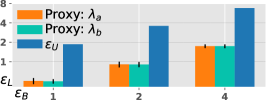
(b)

(c)

(d)

(e)

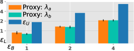
(f)

Figure 1. NTNV setup. Each row corresponds to a different type of differing data $\mathbf{z}$. The vertical axis shows the audited $\varepsilon_{L}$ values based on different proxies. For convenience, the theoretical upper bound $\varepsilon_{U}$ also shares the vertical axis. The horizontal axis is the base algorithm’s (a single run of DP-SGD) privacy budget $\varepsilon_{B}$.

Adversary’s assertion and the lower bound. Adversary’s assertion is exactly the action shown in line 5 in Algorithm 1. Our null and alternative hypothesis are

(9) $$\mathbf{H_{0}}:\text{$X$ was used},\text{\quad}\mathbf{H_{1}}:\text{$X^{\prime}$ was used}.$$

Making assertions means that the adversary needs to transform observations into binary guesses. This is done by forming a real-number proxy and comparing it to some threshold, just like the likelihood ratio test. A base proxy $\lambda_{a}$ will be formed following previous work (nasr2021adversary, ; nasr2023tight, ). Notably, the adversary has access to the score function. Hence, it is reasonable to leverage such additional information. To this end, we will also form a new proxy $\lambda_{b}$ based on the score function. Each of our following sub-experiments will explain $\lambda_{a}$ and $\lambda_{b}$ in detail.

After the adversary makes many assertions, the $FP$ and $FN$ rates are then computed by the Clopper-Pearson method (clopper1934use, ) with a $95\%$ confidence. we then leverage methods proposed in (nasr2023tight, ) to compute the empirical privacy lower bound $\varepsilon_{L}^{(X,X^{\prime},\mathcal{R})}$. We provide detailed procedure for deriving $\varepsilon_{L}^{(X,X^{\prime},\mathcal{R})}$ in Appendix A.3. When the adjacent dataset pair $X,X^{\prime}$ and decision rule $\mathcal{R}$ are clear from the context, we write $\varepsilon_{L}$ instead of $\varepsilon_{L}^{(X,X^{\prime},\mathcal{R})}$.

4.2. Deriving the Lower Bound: Experiments

After formulating the distinguishing game in Section 4.1, we can now conduct experiments to audit the current private hyper-parameter tuning protocol $\mathcal{H}$ (Algorithm 2) under various threat models. Details for the training are provided in Appendix A.3. The audit experiments setup details are summarised in Table 2.

How to assess the privacy of $\mathcal{H}$. We mainly compare various privacy results in this section, and to make the comparison more informative and simpler, we compare $\varepsilon_{L}$ to $\varepsilon_{B}$ and $\varepsilon_{U}$ based on a fixed $\sigma$ value in each setup. Specifically, after we set $\sigma$ for $\mathcal{M}$ at some $\sigma\in\mathbb{R}_{>0}$, we 1) compute $\varepsilon_{B}$ by previous privacy analysis for DP-SGD such as TensorFlow privacy (tfp, ); 2) compute $\varepsilon_{U}$ for $\mathcal{H}$ by current theoretical analysis for hyper-parameter tuning (papernot2021hyperparameter, ); 3) apply privacy audit to $\mathcal{H}$, obtaining $\varepsilon_{L}$ as shown in Section 4.1.

(a)

(b)

(c)

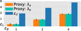
(d)

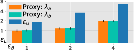
(e)

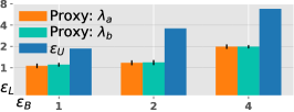
(f)

Figure 2. NTCV setup. Each row corresponds to a different type of differing data $\mathbf{z}$. Axis arrangement is identical to fig. 1.

Normal training and normal validation (NTNV). By the name, this setting is the most practical and normal. The adversary does not control the validation dataset or the score function $g$. Detailed setups are presented in Table 2, row identified by NTNV. Specifically, we have $6$ different settings in this scenario: 1) $X$ is the FASHION dataset, and $\mathbf{z}$ is sampled from MNIST; 2) $X$ is the CIFAR10 dataset, and $\mathbf{z}$ sampled from SVHN; 3) $X$ is the SVHN dataset, and $\mathbf{z}$ is sampled from CIFAR10. $\mathbf{z}$ is chosen from a dataset other than the original training dataset, so the adversary may expect higher distinguishing performance. In the rest settings, $\mathbf{z}=\mathbf{Z}_{D}$ and only $X$ differs.

Note that the score function $g$ is not manipulated in this setup, and the selection behaves normally, i.e., best model is selected if it has the highest score (lowest loss) on the original validation dataset. Hence, we set the proxy as follows. Compute $\mathbf{z}$’s gradient at each iteration before model update: $\{p_{1}^{\mathbf{z}},p_{1}^{\mathbf{z}},\cdots,p_{N}^{\mathbf{z}}\}$, then compute:

(10) $$\lambda_{a}=\frac{1}{N}\sum_{i=1}^{N}\frac{1}{C^{2}}\langle p_{i}^{\mathbf{z}},p_{i}\rangle,{\text{\quad}}\lambda_{b}=\lambda_{a}-g(y),$$

where $\langle a,b\rangle$ is the inner product of two vectors. This follows (nasr2023tight, ) and is based on the design that $p_{i}^{\mathbf{z}}$ is possibly orthogonal to other independent data’s gradient. $\lambda_{b}$ is our newly formed proxy and can be seen as the enhanced version of $\lambda_{a}$ in auditing hyper-parameter tuning because it includes additional information from the score function $g$. By design, higher value of $\lambda_{a}$ or $\lambda_{b}$ incentivizes the adversary to accept $\mathbf{H_{1}}$. The rationale behind these setups is to expect the abnormally differing data (if $X^{\prime}$ is used, or $\mathbf{z}$ was included in the training) to have a detrimental impact on the training so that the model has a higher loss (lower value of $g(y)$), making it more distinguishable if $X^{\prime}$ is used ($\mathbf{z}$ was included in the training).

Results. Experimental results are presented in fig. 1, where we present audited $\varepsilon_{L}$ results corresponding to proxy $\lambda_{a}$ or $\lambda_{b}$. We also present the theoretical upper bound $\varepsilon_{U}$ for comparison. An obvious phenomenon is that the audited $\varepsilon_{L}<\varepsilon_{B}<\varepsilon_{U}$ across all setups shown in the first row of fig. 1. Observing $\varepsilon_{L}<\varepsilon_{U}$ is not so surprising; the interesting phenomenon is that $\varepsilon_{L}<\varepsilon_{B}$ and the gaps between them are obvious. In plain words, this means that the adversary cannot even extract more sensitive information than what the base algorithm’s (a single run) privacy budget allows. This shows the adversary’s power is heavily limited under the most practical setting.

In contrast, in fig. 1(e) and fig. 1(f), when the base algorithm’s privacy budget $\varepsilon_{B}=1$, we see that 1) $\varepsilon_{L}$ is greater than the counterpart in the first row of fig. 1, and 2) $\varepsilon_{L}$ is much closer to $\varepsilon_{B}$. This confirms that the differing data $\mathbf{z}$ that has Dirac gradient gains the adversary more distinguishing power than some natural data. We can also observe that $\lambda_{b}$ has almost no advantage over $\lambda_{a}$, indicating additional information from the score provides limited help, at least when the score function $g$ is not manipulated. Another phenomenon is that the audited $\varepsilon_{L}$ under $\varepsilon_{B}=1$ in fig. 1(d) is weaker than that in fig. 1(e) and fig. 1(f), this suggests that auditing performance depends on $X$.

Normal training and controlled validation (NTCV). In this setting, the adjacent dataset setup is identical to that of NTNV. In contrast, the adversary is relatively stronger: by “controlled validation dataset”, we mean the score function $g$ is manipulated, different from NTNV. We set up two ways of manipulation as follows. 1) The best model is selected based on its loss on some contrived dataset, and we set such dataset to be the differing data $\mathbf{z}$ itself. This corresponds to the first $3$ score function setups in NTCV. 2) There is no action of validation on the model’s prediction; instead, we inspect the first coordinate of the difference vector between the initial model $w_{0}$ and the final model $w_{N}$. This corresponds to the last $3$ score function setups in NTCV. Detailed setups are presented in Table 2, row identified by NTCV.

By design, the rationale behind the first manipulation is to expect the training to memorize the different data $\mathbf{z}$, and the best model is selected based on this metric. The second manipulation builds on the fact that for $\mathbf{Z}_{D}$, it suffices only to investigate the first coordinate of the model to recover any trace of $\mathbf{z}=\mathbf{Z}_{D}$. The proxy $\lambda_{a}$ is identical to that in eq. 10, however, $\lambda_{b}=\lambda_{a}+g(y)$ is set in NTCV, which is different from that in NTNV. This is because $g$ is manipulated. Under the same design considerations, a higher value of $\lambda_{a}$ or $\lambda_{b}$ incentivizes the adversary to accept $\mathbf{H_{1}}$.

Results. Experimental results are presented in fig. 2, and it is organized in a similar manner to fig. 1. We observe a phenomenon similar to NTNV that $\varepsilon_{L}$ sees a big gap to $\varepsilon_{B}$ shown in the first row of fig. 2. In contrast, for the results seen in the second row of fig. 2(e) and fig. 2(f), when base algorithm’s privacy budget $\varepsilon_{B}=1$, we have $\varepsilon_{L}\approx\varepsilon_{B}$. Again, this confirms the Dirac gradient canary is more powerful.

As $g$ is manipulated in this case, it is interesting to compare the performance due to $\lambda_{a}$ and $\lambda_{b}$. We can see that $\lambda_{a}$ and $\lambda_{b}$ have almost the same performance, similar to NTNV where $g$ is not manipulated. It gives more evidence that the score itself provides limited additional help.

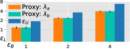
(a)

(b)

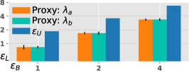
(c)

Figure 3. ETCV setup. Each sub-figure corresponds to a different dataset $X$. Axis arrangement is identical to fig. 1.

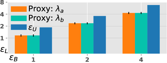
(a)

Figure 4. ETCV setup when $\mathbf{z}\leftarrow\mathbf{Z}_{D}$.

Empty training and controlled dataset (ETCV). Different from both previous settings, we let the training dataset be empty. This means that there is only at most one data sample in the batch $\mathbf{B}$ shown in eq. 1. This setup corresponds to the worst-case dataset mentioned in (nasr2021adversary, ). The adversary can also manipulate the score function in this setting, similar to NTCV. Detailed setups are presented in Table 2, row identified by ETCV.

By design, the rationale behind the empty dataset setup is to eliminate the uncertainties due to normal training data’s gradient so that audit performance is maximized, as the adversary only cares about the causal effect from $\mathbf{z}$ to the output (DBLP:conf/sp/TschantzSD20, ). $\lambda_{a},\lambda_{b}$ are set identically to NTCV. Again, higher value of $\lambda_{a}$ or $\lambda_{b}$ incentivize the adversary to accept $\mathbf{H_{1}}$.

Results. Experimental results are presented in fig. 3 and fig. 4. In fig. 3(a), we can see that $\varepsilon_{L}\approx\varepsilon_{B}$ under all setups; we also notice that $\varepsilon_{L}$ still sees a small gap to $\varepsilon_{B}$ under some setups; however, $\varepsilon_{L}$ gets much closer to $\varepsilon_{B}$ compared with that in NTNV and NTCV. The increased audit performance is due to $X=\emptyset$, which eliminates unwanted disturbances for the adversary.

In fig. 4, when $\mathbf{z}=\mathbf{z}_{D}$ is the Dirac gradient canary instead of some natural data, we observe $\varepsilon_{L}\geq\varepsilon_{B}$ under all setups. This suggests that, operationally, hyper-parameter tuning does leak additional privacy beyond what’s allowed to be disclosed by the base algorithm. This also means that tuning hyper-parameters while only accounting the privacy cost for a single run (i.e., naively taking $\varepsilon_{U}=\varepsilon_{B}$ ) is problematic. On the other hand, like the results in the previous two setups, we also observe that 1) $\lambda_{a}$ and $\lambda_{b}$ have almost the same performance, and 2) there is a big gap between $\varepsilon_{L}$ and $\varepsilon_{U}$.

4.3. Conclusions and Discussions

The weakest audit setup, representative of practical scenarios, reveals that the tuning procedure hardly leaks more privacy even beyond the base algorithm. This suggests a potential safety in tuning hyper-parameters while only accounting for the privacy loss for a single run, aligning with conventional (although not rigorous) practices predating the advent of the generic private selection approach (liu2019private, ; papernot2021hyperparameter, ). While our strongest audit reveals noticeable privacy leakage beyond the base algorithm, it is crucial to note that these findings are confined to worst-case scenarios. Beyond these findings, several noteworthy phenomena emerge, prompting further discussion aimed at achieving a stronger privacy audit on private hyper-parameter tuning.

1) How to instantiate the adjacent dataset pair? Comparing results from NTNV/NTCV with results from ETCV, to reach stronger audit result (higher $\varepsilon_{L}$ value), the adverary clearly favors the worst-case setting, i.e., $X=\emptyset,X^{\prime}=\mathbf{z}$ and $\mathbf{z}$ is adversary-chosen. Note that making assertions in our hypothesis testing problem is equivalent to making assertions on whether $\mathbf{z}$ was included or not included in the training. Hence, only the causal effect from differing data $\mathbf{z}$ to the output is informative to the adversary (DBLP:conf/sp/TschantzSD20, ), and any other independent factors affecting the output will only confuse the adversary to more likely fail the game. Let’s re-investigate eq. 1. Specifically, the clipped gradients of data examples other than $\mathbf{z}$ itself introduce additional unwanted uncertainties to the adversary, making it harder for the adversary to win the distinguishing game, leading to a weaker/smaller lower bound.

2) How to instantiate the differing data $\mathbf{z}$? Compare cases where $\mathbf{z}$ is some real-world data (e.g., $\mathbf{z}=\mathbb{M}[0]$) with cases where $\mathbf{z}=\mathbf{Z}_{D}$, again, the adversary favors the contrived setting. This is because, by restricting the observation to only one dimension, the adversary avoids the uncertainties that are harder to capture under the high-dimension setting, gaining the adversary more distinguishing power. In fact, $\mathbf{z}=\mathbf{Z}_{D}$ suffices to be worst-case, as will be shown in a later section.

Proxy	$\varepsilon_{B}$	$\varepsilon_{U}$	$\varepsilon_{L}$
			NTNV $@$ $X=$			NTCV $@$ $X=$			ETCV $@$ $X=$
			$\mathbb{F}$	$\mathbb{C}$	$\mathbb{S}$	$\mathbb{F}$	$\mathbb{C}$	$\mathbb{S}$	$\emptyset$
$\lambda_{a}$ $\lambda_{b}$	1	1.86	$0.54$ $0.54$	$0.84$ $0.77$	$0.88$ $0.81$	$0.52$ $0.52$	$0.99$ $1.03$	$1.06$ $1.11$	$1.17$ $1.19$
$\lambda_{a}$ $\lambda_{b}$	2	3.59	$0.99$ $1.00$	$1.41$ $1.37$	$1.35$ $1.32$	$0.91$ $0.91$	$1.17$ $1.19$	$1.17$ $1.19$	$2.36$ $2.09$
$\lambda_{a}$ $\lambda_{b}$	4	6.79	$1.91$ $1.91$	$2.13$ $2.13$	$2.13$ $2.13$	$1.74$ $1.74$	$1.99$ $1.98$	$1.99$ $1.98$	$4.28$ $4.68$

Table 3. Results summary for the lower bound $\varepsilon_{L}$ (averaged) obtained due to two different proxies under $\mathbf{z}=\mathbf{z}_{D}$ setup.

3) How does the score function affect audit? This question is of more interest than the previous two because such a question occurs only in auditing $\mathcal{H}$ instead of in previous auditing tasks (auditing the DP-SGD protocol) (nasr2021adversary, ; jagielski2020auditing, ; nasr2023tight, ). We summarise some representative results of our audit experiments in Table 3. First, we observe that $\lambda_{a}$ and $\lambda_{b}$ have similar performance across all setups. Second, by comparing NTNV and NVCT, we see that manipulating the score function does not bring noticeable distinguishing advantages to the adversary.

This phenomenon may seem counter-intuitive and contrasts to the “magic” the adversary may expect: the adversary expects the (distribution of) score of the output when $\mathbf{z}$ is included in the training to be much different from that when $\mathbf{z}$ is not included; hence, manipulating the metric to select the best candidate, should make it much easier for the adversary to succeed the distinguishing game. However, our experimental results diverge from this expectation. The explanation lies in the following observations. $\lambda_{a}$ is computed based on the output resulting from selection by the score function, i.e., the action of selection has already included the score information so that $\lambda_{a}$ has almost the same performance as that of $\lambda_{b}$. Most importantly, the score function itself is differentially private as it is just post-processing. With or without $\mathbf{z}$, the induced score distribution is close to each other, just as what DP guarantees. The “magic” will not happen. This holds for any score function, given it is independent of the sensitive data. Notably, as will be shown in a later section, there is a special type of score function that tends to leak more sensitive information, regardless of whether manipulated or not.

To substantiate this robustness, additional experimental results are presented in Appendix A.5 for reference. A salient observation is that the distribution of scores for the ”best” output remains nearly invariant, regardless of the inclusion or exclusion of $\mathbf{z}$ in the training data, aligning seamlessly with the guarantees provided by differential privacy.

Big gap between $\varepsilon_{L}$ and $\varepsilon_{U}$. In our empirical study, a big gap still exists between $\varepsilon_{U}$ derived by (papernot2021hyperparameter, ) and $\varepsilon_{L}$ obtained even under the strongest adversary. Is it because the adversary is not strong enough? Our following investigation answers this question negatively; instead, $\varepsilon_{U}$ computed by (papernot2021hyperparameter, ) is not tight for private hyper-parameter tuning, and better privacy results can be derived due to the distinct property of the base algorithm (DP-SGD).

5. Improved Privacy Results

Method overview. We are going to find an improved upper bound for protocol $\mathcal{H}$ via eq. 5. Our strategy is as follows. We will first determine the necessary condition for adjacent pair $X,X^{\prime}$. Then, we derive an upper bound for the inner max problem in eq. 5. Instead of finding exact $FP$ and $FN$ rates to derive the privacy parameter, we turn to use divergence-based methods. Specifically, we will leverage the RDP analytical framework.

Worst-case adjacent pair $X,X^{\prime}$. The adjacent pair $X,X^{\prime}$ should be set to be the worst case: $X=\emptyset,X^{\prime}=\mathbf{z}$, as mentioned in Section 4.3. In parallel, such a setup is essentially equivalent to the privacy threat model mentioned in previous works on differential privacy: DP assumes the adversary knows all but one data point, a.k.a. the strong adversary assumption (cuff2016differential, ; li2013membership, ). Knowing all but one data point $\mathbf{z}$ means the adversary can always undo the impact of the data points other than $\mathbf{z}$, which is equivalent to the above worst case. This setup is also implicitly used in previous work that uses analytical approaches to derive the upper bound for the DP-SGD protocol (abadi2016deep, ; rdp_subgaussian_mir, ).

5.1. Reducing the Base Algorithm

To find the upper bound for the tuning protocol $\mathcal{H}$, we clearly need first to understand the privacy of the base algorithm $\mathcal{M}$ as it is the sub-routine of $\mathcal{H}$. Regardless of the differing data $\mathbf{z}$ the adversary may set, we are going to make reductions for the distinguishing game for the base algorithm without impairing the adversary’s power. This is because all reduction is invertible/lossless with respect to information about $\mathbf{z}$ and purely based on the adversary’s knowledge. We first formalize these reductions when the data sampling ratio $\tau=1$, i.e., full-batch gradient decent, no sub-sampling behavior.

First reduction (from eq. 11 to eq. 13). Let $\sigma$ be the coordinate-wise s.t.d. for Gaussian noise shown in eq. 2 to ensure some $(\varepsilon,\delta)$-DP for the base algorithm. And the neural network has $d$ parameters. Based on our above reasoning that $X=\emptyset,X^{\prime}=\mathbf{z}$, then, at each iteration, for the adversary, the private gradient $p_{i}$ is as follows.

(11) $$p_{i}|X=R_{i}\sim\mathcal{N}(0,C^{2}\sigma^{2}\mathbb{I}^{d}),\text{\quad}p_{i}|{X^{\prime}}=(\nabla_{\mathbf{z}}+R_{i})\sim\mathcal{N}(\nabla_{\mathbf{z}},C^{2}\sigma^{2}\mathbb{I}^{d}),$$

where $p_{i}|X$ denotes the random variable conditioned on $X$ was chosen. We also have $\nabla_{\mathbf{z}}=\nabla_{w}\ell(w_{i-1},z)$ and $\|\nabla_{\mathbf{z}}\|_{2}=C$, the gradient of $z$ computed based on last model $w_{i-1}$. The adversary should set the $l_{2}$ norm to be the largest allowable, i.e., $C$. Intuitively, this is because the adversary needs to make the largest impact possible (we will also explain this later). The adversary can always construct a rotational matrix $U_{\mathbf{z}}\in\mathbb{R}^{d\times d}$ such that $p_{i}$ can be reduced as follows.

(12) $$U_{\mathbf{z}}p_{i}|X\sim\mathcal{N}(0,C^{2}\sigma^{2}\mathbb{I}^{d}),\text{\quad}U_{\mathbf{z}}p_{i}|X^{\prime}\sim\mathcal{N}(U_{\mathbf{z}}\nabla_{\mathbf{z}},C^{2}\sigma^{2}\mathbb{I}^{d})$$

where $U_{\mathbf{z}}\nabla_{\mathbf{z}}=[C,0,0,\cdots]^{T}$. This is because Gaussian noise with $\sigma^{2}\mathbb{I}^{d}$ covariance is rotational invariant, i.e.,

$$\|U_{\mathbf{z}}R_{i}\|_{2}=\|R_{i}\|_{2}$$

$$\mathbf{Cov}(U_{\mathbf{z}}R_{i})=U_{\mathbf{z}}\mathbf{Cov}(R_{i})U_{\mathbf{z}}^{T}=C^{2}\sigma^{2}\mathbb{I}^{d}=\mathbf{Cov}(R_{i})$$

where $\mathbf{Cov}(R_{i})$ is the covariance matrix of Gaussian random vector $R_{i}$. After the rotation, for the adversary, only the first coordinate carries useful information about $\mathbf{z}$.

This is because a noise sample $R_{i}\sim\mathcal{N}(0,C^{2}\sigma^{2}\mathbb{I}^{d})$ is coordinate-wise independent, and its rotated version $U_{\mathbf{z}}R_{i}\sim\mathcal{N}(0,C^{2}\sigma^{2}\mathbb{I}^{d})$ possessing $\sigma^{2}\mathbb{I}^{d}$ covariance matrix is also coordinate-wise independent, because uncorrelation implies independence for joint Gaussian. This means that only the first coordinate’s distribution is subject to change based on $X$ or $X^{\prime}$ used; discarding the other coordinates does not impair the adversary’s distinguishing power as they contain no information about $\mathbf{z}$.

In a very intuitive sense, analogously, the first coordinate is the “first-hand” information about $\mathbf{z}$, and it suffices to only consider such information as any further operation on the first coordinate is post-processing. Hence, to serve the distinguishing purpose: $\mathbf{z}$ was/was not used, it suffices to characterize the private gradient $p_{i}$ by $\bar{p}_{i}$ as a univariate random variable as follows.

(13) $$\bar{p}_{i}|X\sim\mathcal{N}(0,C^{2}\sigma^{2}),\text{\quad}\bar{p}_{i}|X^{\prime}\sim\mathcal{N}(C,C^{2}\sigma^{2}).$$

To see why the adversary should enforce the largest $l_{2}$ norm for $\mathbf{z}$’s gradient, we can consider the following: if the $l_{2}$ norm $\|\nabla_{\mathbf{z}}\|_{2}=C^{\prime}<C$, we will arrive at $\bar{p}_{i}|X\sim\mathcal{N}(0,C^{2}\sigma^{2})\text{ and }\bar{p}_{i}|X^{\prime}\sim\mathcal{N}(C^{\prime},C^{2}\sigma^{2})$, This is harder for the adversary to distinguish $\bar{p}_{i}|X$ from $\bar{p}_{i}|X^{\prime}$ as $C^{\prime}<C$ (if $C^{\prime}=0<C$, it is totally indistinguishable).

Second reduction (from eq. 13 to eq. 15). By the first reduction and from the adversary’s view, the DP-SGD’s output $\bar{y}=\{\bar{p}_{1},\bar{p}_{2},\cdots,\bar{p}_{N}\}$ is essentially an observation of $N$ i.i.d. samples from $\mathcal{N}(a,C^{2}\sigma^{2})$ where $a$ is either $0$ or $C$. Recall the adversary’s goal is to distinguish $X$ or $X^{\prime}$ was used; this is equivalent to distinguishing $a=0$ or $a=C$. We can take the average of such $N$ i.i.d. samples as $\bar{y}=\frac{1}{N}\sum_{i=1}^{N}\bar{p}_{i}$ and use it as the final proxy to make the assertion. This operation does not lose any information because the average of such $N$ i.i.d. is sufficient statistics for estimating $a$ (fisher1922mathematical, ; DBLP:books/daglib/0016881, ). Finally, we can reduce the privacy of the base algorithm to an equivalent game for the adversary as

(14) $$\bar{y}|X\sim\mathcal{N}(0,C^{2}\sigma^{2}/N),\text{\quad}\bar{y}|X^{\prime}\sim\mathcal{N}(C,C^{2}\sigma^{2}/N).$$

For mathematical convenience, we apply a simple invertible/lossless re-scaling and arrive at an equivalent characterization:

(15) $$\bar{y}|X\sim\mathcal{N}(0,1),\text{\quad}\bar{y}|X^{\prime}\sim\mathcal{N}(\sqrt{N}/\sigma,1).$$

We let $\mu=\sqrt{N}/\sigma$ for convenience.

When data sampling ratio $\tau<1$. There is only a slight difference in the reduction when $\tau<1$. Instead of arriving at eq. 13, we actually arrive at

(16) $$\bar{p}_{i}|X\sim\mathcal{N}(0,\sigma^{2}),\text{\quad}\bar{p}_{i}|X^{\prime}\sim\mathcal{N}(Cb_{i},\sigma^{2}),$$

where $b_{i},\forall i\in\{1,2,\cdots,N\}$ is independent Bernoulli random variables with probability $\tau$. By doing the same transformation as from eq. 13 to eq. 15, we arrive at

(17) $$\bar{y}|X\sim\mathcal{N}(0,1),\text{\quad}\bar{y}|X^{\prime}\sim\mathcal{N}(\frac{\sum_{i=1}^{N}b_{i}}{N}\sqrt{N}/\sigma,1).$$

We can make good approximations here as $N$ is typically very large in a DP-SGD protocol (e.g., $N>10^{3}$ in (abadi2016deep, )), i.e., $\frac{\sum_{i=1}^{N}b_{i}}{N}\sqrt{N}/\sigma\approx\tau\sqrt{N}/\sigma$ due to law of large numbers. Finally, we arrive at

(18) $$\bar{y}|X\sim\mathcal{N}(0,1),\text{\quad}\bar{y}|X^{\prime}\sim\mathcal{N}(\tau\sqrt{N}/\sigma,1)$$

which also covers eq. 15 when $\tau=1$. A crucial fact is that

(19) $$\mu=\tau\sqrt{N}/\sigma=\Theta(\varepsilon/\sqrt{\log\delta^{-1}})$$

because of eq. 2, i.e., the parameter $\mu$ is independent of any hyper-parameters.

Discussion and summary. We provide discussions for our above reduction in the following.

1) All adversary-chosen $\mathbf{z}$ are equivalent. Our analysis explains the rationale behind the sufficiency of the Dirac gradient canary in our prior empirical investigations as the worst-case scenario. Specifically, it asserts that all adversary-chosen $\mathbf{z}$ instances are equivalent due to the rotational invariance of Gaussian noise and the lossless nature of rotation concerning information pertaining to $\mathbf{z}$.

2) Single parameter characterization. Intuitively, eq. 15 says that distinguishing $X$ or $X^{\prime}$ was used by observing the output of the base algorithm (DP-SGD) is equivalent to distinguishing $\mathcal{N}(0,1)$ from its shifted (by $\mu$) counterpart based on a single draw. The single parameter $\mu$ captures how easily the adversary distinguishes whether $X$ or $X^{\prime}$ was used based on the output of DP-SGD, thereby quantifying the privacy of the DP-SGD protocol.

3) Privacy only depends on the budget. Note that $\mu$ only depends on the privacy budget parameters $\varepsilon,\delta$. This is reasonable because the privacy budget parameter is determined at the very beginning, followed by computing the Gaussian noise s.t.d., which is then determined accordingly to eq. 2. By observing the noisy output of DP-SGD, independent factors, including the hyper-parameters, should never make the adversary easier or harder to win the distinguishing game.

4) Unique property of DP-SGD protocol. The unique property of the DP-SGD protocol is that it typically contains many compositions of Gaussian mechanism ($N$ being very large), which allows us to arrive at the “single parameter characterization”. DP-SGD’s adopting the Gaussian mechanism allows us to make the first reduction, and $N$ being very large allows us to further move from eq. 17 to eq. 18.

5) Relating to Gaussian differential privacy (GDP). Our single parameter characterization for the privacy of the DP-SGD can be linked to Gaussian differential privacy (GDP) (dong2019gaussian, ) by Dong et al., where they also characterize the privacy of some algorithms as the game of distinguishing two univariate Gaussians. GDP is provided in Appendix A.4 for reference. In fact, the claim in (dong2019gaussian, ) is much stronger: as long as some arbitrary algorithm $\mathcal{M}$ has many compositions (not necessarily of Gaussian mechanism) and satisfies some properties (which are met by DP-SGD (dong2019gaussian, )), the privacy of $\mathcal{M}$ can be characterized by GDP, i.e., a single parameter characterization. The reason behind such a fact is the central limit behavior due to many compositions (dong2019gaussian, ), which is also explained in Appendix A.4. In (dong2019gaussian, ), they provide another approach to computing the $\mu$ parameter, essentially similar to what we have done in eq. 19.

Our improved results in later sections will require $\mu$ as input. In addition to our method for deriving $\mu$, we will also leverage GDP’s method to compute $\mu$.

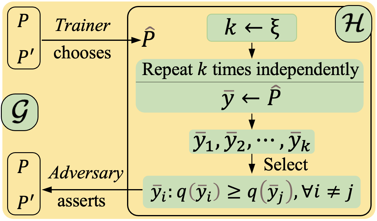
Figure 5. The reduced distinguishing game $\mathcal{G}$ for private hyper-parameter tuning. Two univariate Gaussian distributions $P$ and $P^{\prime}$ correspond to adjacent dataset pair $X,X^{\prime}$. At each execution of $\mathcal{G}$, The trainer chooses one distribution and feeds it to the private hyper-parameter tuning routine $\mathcal{H}$; then an integer $k>0$ is sampled from $\xi$ followed by independently sampling $k$ times from $\hat{P}$. After getting such $k$ samples $\{\bar{y}_{1},\bar{y}_{2},\cdots,\bar{y}_{k}\}$, a best sample $\bar{y}_{i}$ is selected based on a score evaluator $q:\mathbb{R}\rightarrow\mathbb{R}$ and returned to the adversary. Finally, the adversary asserts which distribution was chosen.

5.2. Reducing the Tuning Protocol

In this section, we are going to reduce the distinguishing game for $\mathcal{H}$ based on our previous reduction for the base algorithm. We formalize the reduced version of the distinguishing game $\mathcal{G}$ for private hyper-parameter tuning $\mathcal{H}$ in fig. 5. We abstract a single run of a DP-SGD protocol, which outputs a sample $y$, as sampling $\bar{y}$ from a univariate Gaussian. This treatment comes with no information loss with respect to $\mathbf{z}$, as shown by our reduction on the base algorithm. To analyze the privacy problem for the reduced result, there remains only one missing part: the score evaluator $q$.

Constructing the worst-case score evaluator $q$. $q:\mathbb{R}\rightarrow\mathbb{R}$ is the counterpart of the score function $g$ mentioned before. It now suffices to investigate the distribution of the best sample $\bar{y}_{i}|P$ and $\bar{y}_{i}|P^{\prime}$ induced by $q$ shown in fig. 5. We denote the $\bar{y}_{i}|P$ as the distribution conditioned on $P$ was chosen. A naive attempt is first to find the exact relationship between the original score function $g$ and $q$, which can be very complex and then bound the RDP $\mathcal{D}_{\alpha}(\bar{y}_{i}|P||\bar{y}_{i}|P^{\prime})$. Fortunately, we do not need to know such a relationship. Our goal is to find an RDP upper bound; hence, we only need to find the worst-case $q$ in the reduced problem. First, we introduce the following theorem to show the necessary conditions for the worst-case score evaluators.

Theorem 1 (One-to-one Mapping Makes It Most Distinguishable).

Let distribution $P$ be over some finite alphabets $\Gamma$, and define a distribution $F_{k,q}$ as follows. First, make $k>0$ independent samples from $P$: $\{x_{1},x_{2},\cdots,x_{k}\}$, then output $x_{i}$ such that the score $r=q(x_{i})$ computed by a score evaluator $q:\Gamma\rightarrow\mathbb{R}$ is the maximum over these samples. Similarly, we define another distribution $P^{\prime}$ over the same alphabet, and we obtain distribution $F^{\prime}_{k,q}$ as the counterpart of $F_{k,q}$. For any score evaluator $\hat{q}$, which is not a one-to-one mapping, i.e., it needs a tie-breaking, and we enforce random (can be arbitrarily weighted) selection among alphabets sharing identical score if any of them is sampled. Consequently, there always exists a one-to-one mapping $q^{*}$ satisfying the following.

(20) $$\mathcal{D}_{\alpha}(F_{k,\hat{q}}||F^{\prime}_{k,\hat{q}})\leq\mathcal{D}_{\alpha}(F_{k,q^{*}}||F^{\prime}_{k,q^{*}}).$$

The proof is provided in Appendix B.2. This simple form of equation essentially tells us crucial facts: a non-one-to-one mapping $q$ by which to select and return the maximum tends to make the output more private in RDP sense, i.e., with smaller RDP value. In plain words, a score evaluator/function that induces a strict total order for elements in $\Gamma$ tends to leak more information. This is not hard to understand. For instance, if the score evaluator can only output a constant, then the selection is purely random, which gains the adversary no additional advantage. In principle, computing a score is post-processing, and a one-to-one mapping does not lose any information, hence better serving the adversary’s distinguishing goal. Moreover, when $k$ follows a general distribution, we also have the same results shown in the following.

Corollary 0.

Denote $F_{\xi,\hat{q}},F^{\prime}_{\xi,\hat{q}},F_{\xi,q^{*}},F^{\prime}_{\xi,q^{*}}$ as the counterpart distributions to those in Theorem 1 when $k$ follows a general distribution $\xi$ instead of being a fixed number, the result in Theorem 1 still holds, i.e.,

$$\mathcal{D}_{\alpha}(F_{\xi,\hat{q}}||F^{\prime}_{\xi,\hat{q}})\leq\mathcal{D}_{\alpha}(F_{\xi,q^{*}}||F^{\prime}_{\xi,q^{*}}).$$

The proof follows Theorem 1 and is provided in Appendix B.3. In fact, we can extend the above results to the case where distribution $P,P^{\prime}$ is over some domain $\Gamma$ which is infinite (e.g., $\Gamma=\mathbb{R}$) because Rényi divergence can be approximated arbitrarily well by finite partition as shown by Theorem 10 in (van2014renyi, ).

Continuous score evaluator $q$. Now we can restrict to all one-to-one mappings score evaluators $q:\mathbb{R}\rightarrow\mathbb{R}$. Note that infinitely many one-to-one mappings exist, but the above result does not tell us which to consider. Fortunately, we can just focus on continuous ones. This corresponds to $q$’s counterpart, the original score function $g$, being continuous. This is due to both practical and analytical considerations. For instance, $g$ in real applications is often continuous, e.g., the loss on a validation dataset, the Perplexity score (jelinek1977perplexity, ) for language models, etc. The accuracy of a validation dataset is not continuous, which makes analysis difficult; however, the loss is just a differentiable proxy for the accuracy, sidestepping such difficulty. In principle, we essentially require that the original score function $g$ is “stable”, i.e., a small perturbation in its input does not incur a drastic change in the output. We believe such property is also what a natural/useful score function should have in practice.

In our discussion, being continuous for one-to-one mapping $q$ means that $q:\mathbb{R}\rightarrow\mathbb{R}$ is either strictly increasing or decreasing because continuous one-to-one mapping implies monotone. As the following shows, we know we can just focus on the simplest one $q(x)=x$.

Proposition 0.

$q_{1},q_{2}:\mathbb{R}\rightarrow\mathbb{R}$ are two strictly increasing score functions. Denote $\mathcal{N}_{\xi,q_{1}},\mathcal{N}^{\prime}_{\xi,q_{1}},\mathcal{N}_{\xi,q_{2}},\mathcal{N}^{\prime}_{\xi,q_{2}}$ as the counterpart distributions to those in corollary 2 such that $P=\mathcal{N}(0,1),P^{\prime}=\mathcal{N}(\mu,1)$ for some $\mu$ shown in eq. 19. We have

$$\mathcal{D}_{\alpha}(\mathcal{N}_{\xi,q_{1}}||\mathcal{N}^{\prime}_{\xi,q_{1}})=\mathcal{D}_{\alpha}(\mathcal{N}_{\xi,q_{2}}||\mathcal{N}^{\prime}_{\xi,q_{2}}).$$

The same is also true if $q_{1},q_{2}$ are strictly decreasing.

The proof is provided in Appendix B.4. This says that all strictly increasing functions are equivalent to the adversary. The truth of proposition 3 is almost self-evident. Because both the output $\bar{y}_{i}$ under $q_{1}$ and output $\bar{y}_{i}$ under $q_{2}$ contain the same information exactly: the final output observed by the adversary is the largest among all sampled ones. Due to symmetry, we only need to consider strictly increasing ones, i.e., $q(x)=x$ will suffice, and we will omit the notation for $q$ in the following.

5.3. Compute Improved Privacy Results

Now, we are able to compute the privacy RDP upper bound $\mathcal{D}_{\alpha}(\bar{y}_{i}|P||\bar{y}_{i}|P^{\prime})$ for the reduced game shown in fig. 5. Deriving a general closed-form solution analytically seems infeasible because the distribution considered is a mixture, and the random variable $k$’s distribution can be arbitrary. This makes us resort to numerical approaches. Our strategy is presented as Algorithm 3.

As shown in Algorithm 3, our method requires the input of the single privacy parameter $\mu$, which is computed by our reduction shown in eq. 19 or GDP (papernot2021hyperparameter, ) shown in corollary 7. When $\xi$ is a point mass on $k$, the distribution of $\mathcal{N}_{\xi}$ is well studied in order statistics, i.e., it is the distribution of the maximum over $k$ independent samples drawn from $\mathcal{N}(0,1)$. This explains the term $kF(x)^{k-1}f(x)$. When $k$ itself is random, we obtain a mixture as shown in line 3 and 4 in Algorithm 3. In plain words, the overall distinguishing game for the adversary based on the $\mathcal{H}$’s output is distinguishing $\mathcal{N}_{\xi}$ from $\mathcal{N}^{\prime}_{\xi}$. The last step in Algorithm 3 is due to the symmetry of adjacency. To convert to the $(\varepsilon,\delta)$-DP form, we apply Theorem 20 in (balle2020hypothesis, ) (shown in Appendix A.2).

Algorithm 3 Compute RDP For the Reduced Game in fig. 5

1:Distribution $\xi$; the single privacy parameter $\mu$

2:$F(x)\leftarrow\text{ c.d.f. of }\mathcal{N}(0,1)$, $f(x)\leftarrow\text{ p.d.f. of }\mathcal{N}(0,1)$

3:$\mathcal{N}_{\xi}(x)\leftarrow\mathbb{E}_{k\sim\xi}[kF(x)^{k-1}f(x)]$$\triangleright$ Due to $\mathcal{N}(0,1)$

4:$\mathcal{N}^{\prime}_{\xi}(x)\leftarrow\mathbb{E}_{k\sim\xi}[kF(x-\mu)^{k-1}f(x-\mu)]$$\triangleright$ Due to $\mathcal{N}(\mu,1)$

5:$\gamma=\max\{\mathcal{D}_{\alpha}(\mathcal{N}_{\xi}||\mathcal{N}^{\prime}_{\xi}),\mathcal{D}_{\alpha}(\mathcal{N}^{\prime}_{\xi}||\mathcal{N}_{\xi})\}$

6:$\gamma$

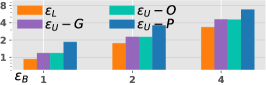
(a)

(b)

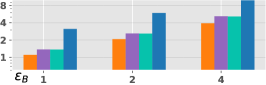
(c)

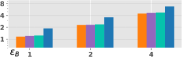
(d)

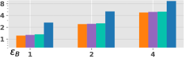
(e)

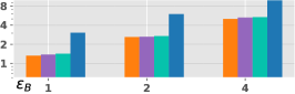
(f)

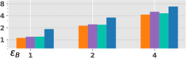
(g)

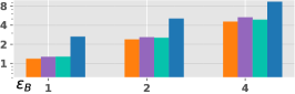
(h)

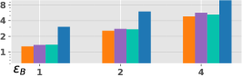
(i)

Figure 6. Comparison of various privacy results for $\mathcal{H}$ (Algorithm 2). Our method for deriving the privacy upper bound is labeled as $\varepsilon_{U}-G$ and $\varepsilon_{U}-O$. $\varepsilon_{L}$ is the result of the privacy audit. Previous generic upper bound (papernot2021hyperparameter, ) is labeled as $\varepsilon_{U}-P$. The horizontal axis is the base algorithm’s privacy budget ($\varepsilon_{B}$). Each row corresponds to different sample ratios $\tau$, and each column corresponds to different $\xi_{\eta,\nu}$, the TNB distribution shown in section A.1. The base algorithm (the DP-SGD protocol) has $N=500$ iterations, and all privacy results are based on $\delta=10^{-5}$.

5.4. Privacy Results Evaluation

In this part, 1) we present our privacy results. Compared with the generic privacy bound for private hyper-parameter tuning in (papernot2021hyperparameter, ), we show our result is better under various settings. 2) We apply privacy audit to find the lower bound, showing that our privacy results are nearly tight. Results are presented at fig. 6.

In fig. 6, Previous privacy theoretical upper bound is labeled as $\varepsilon_{U}-P$. The privacy upper bound derived by our method includes two variants, and they are labeled as $\varepsilon_{U}-G$ and $\varepsilon_{U}-O$. The former corresponds to using GDP (dong2019gaussian, ) to compute the single private parameter $\mu$ input to Algorithm 3. The latter corresponds to using Our reduction shown in Section 5.1 to compute $\mu$, i.e., eq. 19. $\varepsilon_{L}$ is the result of the privacy audit, presented to assess the tightness of our method. The setup of this auditing experiment is summarised as follows.

Lower bound by efficient privacy audit. Auditing private learning is expensive because the training is computationally intensive; however, since the above problem has been reduced to be simple (as shown in fig. 5), audit becomes cheap: in analogous, a sampling from a Gaussian $\hat{P}$ is like a run of $\mathcal{M}_{i}$ (Algorithm 2) in our previous empirical study. This means that we can even carry out the simulation for fig. 5 millions of times. In this audit experiment, the setup is quite simple: 1) the adversary takes the output sample $\bar{y}_{i}$ as the proxy to make assertions/guesses $b_{guess}$; 2) we simulate fig. 5 $10^{6}$ times; 3) and next processes of concluding $\varepsilon_{L}$ just follows the general procedures shown in Appendix A.3.

In fig. 6, we can see that for all $\tau$ values, the privacy results derived by our method have a significant advantage (much tighter) over the generic bound $\varepsilon_{U}-P$. Under $\tau=1$, the lower bound found by privacy audit still sees a noticeable disparity from our privacy results; however, when $\tau$ is smaller, the gap almost vanishes, indicating our privacy results are almost tight.

Generalizability. The privacy results in previous work can only easily apply when $\xi$ is some specific distribution: Liu et al. (liu2019private, ) assume $\xi$ is the geometric distribution, and Steinke et al. (papernot2021hyperparameter, ) give results for $\xi$ to be the TNB distribution and Poisson distributions. When $\xi$ is some other distribution, it seems like substantial analytical work is further needed to adopt previous results. In contrast, our result is more versatile and is applicable to arbitrary distribution, as we made no assumptions for $\xi$. To this end, we provide an application in Appendix A.5 to show that our results easily apply to a very simple distribution $\xi$, which seems to require additional analytical work to adopt the approaches in (liu2019private, ; papernot2021hyperparameter, ).

6. Discussion

Why does hyper-parameter tuning enjoy a better privacy bound? This question pertains to a fundamental aspect of privacy quantification. In (papernot2021hyperparameter, ) that proposes the current state-of-the-art privacy bound for the private selection problem, the privacy analysis is within the RDP framework, and the privacy bound for the tuning problem $\mathcal{H}$ can be derived as long as each base algorithm $\mathcal{M}_{i}$ is some $(\alpha,\gamma)$-RDP. However, the intrinsic limitation of RDP lies in the possibility that distinct private mechanisms might share the same $(\alpha,\gamma)$-RDP bound. For example, a Randomized Response (RR) mechanism and the Gaussian mechanism (GM) may satisfy the same RDP under some setup (zhu2022optimal, ), despite their inherent dissimilarity. This underscores that RDP, while widely utilized, is not perfectly informative for privacy quantification.

In contrast, $f$-DP (dong2019gaussian, ), a more sophisticated hypothesis-testing-based privacy quantification provided in Appendix A.4, offers a finer resolution in capturing discrepancies between mechanisms. It has been shown in (zhu2022optimal, ) that $f$-DP captures the discrepancies between RR and GM, although they satisfy the same RDP.

We mentioned that the unique property of DP-SGD, i.e., it has many compositions of GM, makes the hyper-parameter tuning enjoy a better privacy analysis. This stems from the fact that DP-SGD’s privacy is characterized by GDP, which corresponds to a unique $f$-DP characterization (see Appendix A.4), and a base algorithm satisfying GDP enjoys a better bound in the private selection problem, just as we demonstrated previously. The reduction we made in Section 5.1 can be seen as a dual perspective to GDP.

The worst-case example provided in Example 1 may satisfy some RDP bound identical to some DP-SGD instance; however, it does not possess the same $f$-DP as that of DP-SGD, hence not enjoying a better bound in the private selection problem. When treating the base algorithm as a black box, the generic privacy bound in (papernot2021hyperparameter, ) for private selection is demonstrated to be tight, as illustrated in Example 1. However, more favorable privacy results can be attained when the base algorithm is scrutinized in a white-box manner.

7. Conclusion

We investigate the current state-of-the-art privacy bound for private selection problems. Initially, we give examples showing that the current generic bound is indeed tight in general. However, such tightness does not apply to hyper-parameter tuning problems due to the distinct properties of the base algorithm (DP-SGD). Substantiating this assertion, we first conduct empirical studies for the private tuning problem under various privacy audit setups. Our findings reveal that, in certain practical scenarios, a weak adversary can only acquire restricted sensitive information. For the strongest adversary, the derived empirical privacy bound still sees a significant gap from the current generic bound. We then take further steps to analyze the privacy issues in hyper-parameter tuning and derive better privacy results. Compared with the current generic bound, our result is better under various settings. By conducting further audit experiments, we show that our result is nearly tight. In addition, our analysis does not depend on $\xi$, contrasting to previous work where their results are only easily applicable to specific $\xi$ distributions.

Appendix A Content for reference

A.1. Privacy Results by Steinke et al.

Truncated negative binomial (TNB) distribution. For $\nu\in(0,1)$ and $\eta\in(-1,\infty)$, the distribution $\xi_{\eta,\nu}$ on $\{1,2,3,\cdots\}$ is as follows. When $\eta\neq 0$, then

$$\forall k\in\mathbb{N},\quad\operatorname{Pr}[K=k]=\frac{(1-\nu)^{k}}{\nu^{-\eta}-1}\cdot\prod_{\ell=0}^{k-1}\left(\frac{\ell+\eta}{\ell+1}\right),$$

when $\eta=0$, then

$$\forall k\in\mathbb{N},\quad\operatorname{Pr}[K=k]=\frac{(1-\nu)^{k}}{k\cdot\log(1/\nu)}$$

This particular distribution is obtained by differentiating the probability generating function of some desired form [40]. The main relevant privacy results in [40] are provided in the following. Note that they are all in RDP form.

Theorem 1 (TNB distribution [40]).

Let $k$ in Algorithm 1 follows TNB distribution $\xi_{\eta,\nu}$. If the base algorithm satisfies $(\alpha,\gamma)$-RDP and $(\alpha^{\prime},\gamma^{\prime})$-RDP, Algorithm 1 satisfies $(\alpha,\hat{\gamma})$-RDP where

$$\hat{\gamma}=\gamma+(1+\eta)\cdot\left(1-\frac{1}{\alpha^{\prime}}\right)\gamma^{\prime}+\frac{(1+\eta)\cdot\log(1/\nu)}{\alpha^{\prime}}+\frac{\log\mathbb{E}_{\xi_{\eta,\nu}}}{\alpha-1}$$

Theorem 2 (Poisson distribution [40]).

Let $k$ in Algorithm 1 follow Poisson distribution with mean $\mu$. If the base algorithm satisfies $(\alpha,\gamma)$-RDP and $(\varepsilon^{\prime},\delta^{\prime})$-DP; and if $e^{\varepsilon^{\prime}}\leq 1+\frac{1}{\alpha-1}$, Algorithm 1 satisfies $(\alpha,\hat{\gamma})$-RDP where

$$\hat{\gamma}=\gamma+\mu\cdot\delta^{\prime}+\frac{\log\mu}{\alpha-1}$$

Note that $(\varepsilon,0)$-DP is equivalent to $(\infty,\varepsilon)$-RDP; Therefore, $\eta=1$ in [40] recovers the case in [28] and $\eta<1$ leads to improved results compared with [28].

Tight example for approximate DP The tight example for approximate DP case can be obtained with a trick trivially based on our pure DP example shown in example 1. If an algorithm is $(\varepsilon,0)$-DP, it is also $(\varepsilon,\delta)$-DP. Hence, the above tight example covers the $(\varepsilon,\delta)$-DP case. Specifically, it can be checked that the example shown in eq. 6 is $(1,10^{-5})-DP$ and eq. 8 is $(2.92,10^{-5})$-DP. Compared to the result predicted by [40], which is $(3.11,10^{-5})$-DP, we also see that it is tight up to a negligible gap.

A.2. Conversion From RDP to DP

Theorem 3 ([4]).

For $\alpha>1$ and $\delta>0$, and for a mechanism $\mathcal{M}$ which is $(\alpha,\gamma)$-RDP, then it satisfies $(\varepsilon,\delta)$-differential privacy where

$$\varepsilon=\gamma+\log\frac{\alpha-1}{\alpha}-\frac{\log\delta+\log\alpha}{\alpha-1}.$$

This conversion is adopted by TensorFlow privacy [1].

A.3. Used Datasets and Experimental Details

Our implementation is provided at an anonymous link. We use four image datasets in our experiments. FASHION [49], MNIST [26], CIFAR10 [25] and SVHN [38]. We simply let $I=0$ throughout our experiments, shown in Table 2. All of our experiments are conducted under privacy parameter $\delta=10^{-5}$ and we vary $\varepsilon$ to be $\{1,2,4\}$. The number of repeating/simulation times in an audit experiment is $2,000$. The error bar is the result of taking the maximum, minimum, and average for three trials. To efficiently audit the hyper-parameter tuning and reduce the simulation burden, we only fetch 5,000 data examples from the original training datasets, and we set the sampling rate to be 1, i.e., full gradient decent. Our audit experiment consumes $>4000$ GPU-hours and is conducted over 20 GPUs in parallel.

Detailed procedure of concluding the lower bound $\varepsilon_{L}$. The following procedure is adopted to conclude a lower bound $\varepsilon_{L}$.

1) Forming $(b_{truth},b_{guess})$. Each pair corresponds to an execution of $\mathcal{G}$ (Algorithm 1). The adversary needs to make an assertion, i.e., output a $b_{truth}\in\{0,1\}$, this is done by comparing some proxy $\lambda$, e.g., like $\lambda_{a},\lambda_{b}$ we formed in our experiments, to a threshold $th$. The adversary outputs $b_{truth}=1$ if $\lambda>th$, $b_{truth}=0$ otherwise.

2) Compute $\varepsilon_{L}$. After getting many pairs of $(b_{truth},b_{guess})$, the $FP,FN$ rates can be summarised by Clopper-Pearson with a confidence $c$. Specifically, the $FP$ rate and $FN$ rate are modeled as the unknown success probabilities of two binomial distributions. Then $\varepsilon_{L}$ can be computed by eq. 4 or by the methods used in [35].

3) Optimization. In practice, practitioners often use various thresholds to find the optimal, e.g., by observing the largest proxy $\lambda_{max}$ and the smallest $\lambda_{min}$, $th$ candidates can be set to be numbers that uniformly dividing interval $[\lambda_{min},\lambda_{max}]$. Repeating procedures 1) and 2) with different $th$ values, we may select the one leading the largest $\varepsilon_{L}$ value.

A.4. Gaussian Differential Privacy (GDP)

Definition 0 (Trade-off function [14]).

For any two distribution $P,Q$, define the trade-off function as:

$$T(P,Q)(FP)=\inf_{\mathcal{R}}\{FN_{\mathcal{R}}:FP_{\mathcal{R}}\leq FP\}$$

where the infimum is taken over all rejection rule $\mathcal{R}$.

The trade-off function clearly characterizes the boundary of achievable and unachievable type I error ($FP$) and type II error ($FN$). We say $f\geq g$ if $f(x)\geq g(x),\forall x\in[0,1]$.

Definition 0 ($f$-differential privacy ($f$-DP)[14]).

Let $f:[0,1]\rightarrow[0,1]$ be a trade-off function. A mechanism $\mathcal{M}$ satisfies f-DP if

$$T(\mathcal{M}(X),\mathcal{M}(X^{\prime}))\geq f$$

for all adjacent dateset pair $X,X^{\prime}$

This means that the distinguishing game corresponding to $\mathcal{M}$ is harder than the one underlying $f$. $f$-DP captures the privacy of some private algorithms by the functional relationship between $FP$ and $FN$, which is shown to be more expressive than RDP [52].

Definition 0 ($\mu$-Gaussian differential privacy ($\mu$-GDP) [14]).

A privacy mechanism $\mathcal{M}$ is $\mu$-GDP if

$$T(\mathcal{M}(X),\mathcal{M}(X^{\prime}))(FP)\geq\Phi(\Phi^{-1}(1-FP)-\mu)$$

holds for all adjacent dataset pair $X,X^{\prime}$. $\Phi$ is the c.d.f. of standard normal distribution.

The nice property of GDP is that it exactly characterizes the privacy of the Gaussian mechanism. Moreover, the GDP also characterizes the privacy of a mechanism that contains many compositions due to the central limit theorem. For the DP-SGD protocol shown in eq. 1, if the sampling ratio for each data inside $\mathbf{B}$ is $\tau$ and the total iteration number is $T$, we have the following.

Corollary 0 (GDP approximation for DP-SGD [14]).

If $\tau\sqrt{T}\rightarrow c$ for some constant $c$, then DP-SGD is asymptotically $\mu$-GDP with

$$\mu=\sqrt{2}c\cdot\sqrt{\mathrm{e}^{\sigma^{-2}}\cdot\Phi\left(1.5\sigma^{-1}\right)+3\Phi\left(-0.5\sigma^{-1}\right)-2}.$$

where $\sigma=\sigma^{\prime}/C$ and $\sigma^{\prime}$ is s.t.d. of the Gaussian noise, $C$ is the clipping threshold.

As shown in [14], this approximation is very accurate (with respect to $f$-DP characterization) given $T$ large enough and $\tau$ small enough.

Central limit behavior leading to GDP. Instead of elaborating on the rather technical reasoning shown in the original paper [14], we provide a different but more intuitive explanation for the central limit behavior possessed by an algorithm that has many compositions.

We can characterize the privacy of a single composition by the Privacy Loss Random Variable (PRV) [18] whose distribution is called Privacy Loss Distribution (PLD). For any DP mechanism, a PRV can be derived for that algorithm. The nice property of PRV is that under adaptive composition, the overall privacy is captured by just adding up all the PRVs. For DP-SGD protocol shown in eq. 1, all PRVs are i.i.d.. Hence, when the number of compositions is large enough, the PRV for the whole mechanism (the sum of many i.i.d. random variables) exhibits central limit behavior. This means that, as long as the number of compositions is large enough, all DP-SGD instance converges to a case which is uniquely formalized by GDP in [14].

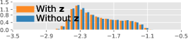
(a)

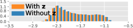
(b)

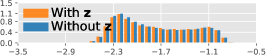
(c)

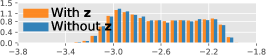
(d)

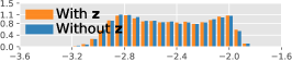
(e)

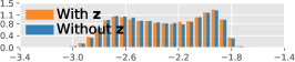
(f)

Figure 7. The output’s score histogram under NTNV setup. The first and second rows correspond to the Fashion and CIFAR10 training datasets, respectively. Each column corresponds to a different base algorithm’s privacy budget $\varepsilon_{B}$. The scores are validation loss over the original normal validation dataset, i.e., not manipulated.

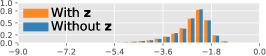
(a)

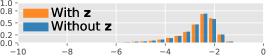
(b)

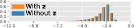
(c)

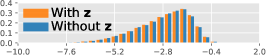
(d)

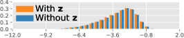
(e)

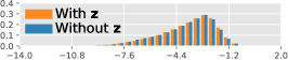
(f)

Figure 8. The output’s score histogram under NTCV setup. Each row corresponds to a different training dataset, and each column corresponds to a different base algorithm’s privacy budget $\varepsilon_{B}$. The score function is the validation loss over $\mathbf{z}$, i.e., manipulated.

(a)

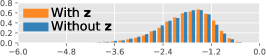
(b)

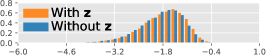
(c)

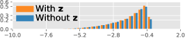
(d)

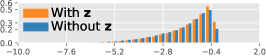
(e)

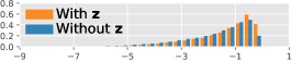
(f)

Figure 9. The output’s score histogram under ETCV setup. Each row corresponds to a different training dataset, and each column corresponds to a different base algorithm’s privacy budget $\varepsilon_{B}$. The score function is the validation loss over $\mathbf{z}$, i.e., manipulated.

$\varepsilon_{B}$	$\tau$	$L=10$ $s=10^{-1}$	$L=10$ $s=10^{-2}$	$L=100$ $s=10^{-2}$	$L=100$ $s=10^{-3}$	$L=1000$ $s=10^{-3}$
1	1	$1.13$ $1.12$	$1.29$ $1.28$	$2.58$ $2.57$	$3.34$ $3.33$	$5.42$ $5.40$
	0.5	$1.13$ $1.12$	$1.30$ $1.28$	$2.59$ $2.57$	$3.36$ $3.33$	$5.43$ $5.40$
	0.1	$1.13$ $1.08$	$1.30$ $1.24$	$2.59$ $2.49$	$3.36$ $3.23$	$5.44$ $5.25$
2	1	$2.23$ $2.21$	$2.39$ $2.38$	$4.28$ $4.25$	$5.56$ $5.53$	$8.27$ $8.23$
	0.5	$2.25$ $2.21$	$2.41$ $2.38$	$4.30$ $4.25$	$5.59$ $5.53$	$8.31$ $8.23$
	0.1	$2.40$ $2.19$	$2.56$ $2.36$	$4.48$ $4.23$	$5.83$ $5.50$	$8.57$ $8.20$
4	1	$4.51$ $4.43$	$4.52$ $4.44$	$5.93$ $5.90$	$7.85$ $7.80$	$10.22$ $10.20$
	0.5	$4.51$ $4.35$	$4.52$ $4.37$	$5.93$ $5.88$	$7.85$ $7.76$	$10.22$ $10.18$
	0.1	$4.96$ $4.15$	$4.98$ $4.16$	$6.15$ $5.79$	$8.05$ $7.63$	$10.27$ $10.12$

Table 4. Our improved privacy results under different setups for the simple distribution $\xi$ shown in eq. 21. For data in each cell, the first row is $\varepsilon_{U}-G$, and the second row is $\varepsilon_{U}-O$. For all results, we set $\delta=10^{-5}$ and $N=500$.

A.5. More Experimental Results

Measuring the score distribution. To confirm the robustness mentioned above. A straightforward way is to inspect the scores of the output of $\mathcal{H}$ (Algorithm 2). What we expect should happen is that whether $\mathbf{z}$ is included in the training or not (corresponding to $X,X^{\prime}$), the score distribution should not change much because of DP’s guarantee. We make the measurement for two different training datasets, and results are presented in In fig. 7. We process the scores by shifting so that all scores are $<0$. Our result clearly shows no significant difference between the score distributions when $\mathbf{z}$ is included ($X^{\prime}$ is used) and when it is not included ($X$ is used) in the training. In fig. 8 and fig. 9, we again obverse the “indistinguishability” between cases where $\mathbf{z}$ is included and cases where $\mathbf{z}$ is not. Such robustness holds no matter whether the score function is manipulated or not.

Applications of our results. We can apply our results to more general applications based on such facts. For example, to avoid possible complexities in sampling from $\xi$ when $\xi$ itself is complicated, we can now let $\xi$ to be a very simple and intuitive binary distribution:

(21) $$\xi:\left\{\begin{array}[]{ll}\operatorname{Pr}[K=1]=s\\ \\ \operatorname{Pr}[K=L]=1-s\\ \end{array}\right.$$

where $L$ can be set as some large integer and $s<1$ can be set as some small value. This setup ensures we have a high probability of running the base algorithm enough times to find good hyper-parameter configurations (i.e., for utility reasons).

Somewhat surprisingly, even when $L$ is large and $s$ is small, the privacy still deteriorates modestly. This is still possibly due to the unique property of DP-SGD, i.e., it contains many compositions of Gaussian mechanisms. We present our privacy results under various settings in Table 4.

Appendix B Proofs

B.1. Proof of Theorem 2

Proof.

when $k>0$ is some fixed number, we know that the scores of all $k$ runs are all less than or equal to $g(y)$, which has the probability $\operatorname{Pr}(E_{\leq y})^{k}$. As $y$ occurs, we must rule out the probability of $y$ occurring zero times, which is $\operatorname{Pr}(E_{<y})^{k}$. Hence, we have probability $\operatorname{Pr}(E_{\leq y})^{k}-\operatorname{Pr}(E_{<y})^{k}$ seeing $y$ as the output of Algorithm 2. When $k$ follows distribution $\xi$, all of the above probability becomes a mixture of distributions, leading to Theorem 2. ∎

B.2. Proof of Theorem 1

Proof.

W.o.l.g., we define the alphabets of distribution $P$ and $P^{\prime}$ as $\{a,b,c,d,e,f\}$, with some abuse of notation, we denote

$$P(a)=p_{a},P(b)=p_{b},\cdots,P(f)=p_{f}$$

$$P^{\prime}(a)=p^{\prime}_{a},P^{\prime}(b)=p^{\prime}_{b},\cdots,P^{\prime}(f)=p^{\prime}_{f}$$

as their probabilities. Suppose we have a non-one-to-one mapping score evaluator $\hat{q}$ such that:

$$\hat{q}(a)=\hat{q}(c)=\hat{q}(e)<\hat{q}(b)=\hat{q}(d)<\hat{q}(f).$$

For ease of discussion and simplicity, we now assume a uniformly random selection among Alphabets that share the same score. This means that they share the same probability of being outputted.

In fact, for alphabets sharing the same score, the selection is not necessarily uniformly random, e.g., they can be selected in a fashion weighted by their own probability mass. This does not make any difference to the utility, as the output’s score stays the same. Additionally, our final conclusion still holds no matter whether it is uniform or weighted because our key step does not assume whether it is uniform or weighted. For clearer presentation, we denote $\Lambda_{S}^{k}=(\sum_{i\in S}p_{i})^{k}$ and $\bar{\Lambda}_{S}^{k}=(\sum_{i\in S}p^{\prime}_{i})^{k}$.

Then, the distribution of $F_{k,\hat{q}}$ will be

$$F_{k,\hat{q}}(a)=F_{k,\hat{q}}(c)=F_{k,\hat{q}}(e)=\frac{1}{3}\Lambda_{\{a,c,e\}}^{k}$$

$$F_{k,\hat{q}}(b)=F_{k,\hat{q}}(d)=\frac{1}{2}(\Lambda_{\{a,c,e,b,d\}}^{k}-\Lambda_{\{a,c,e\}}^{k})$$

$$F_{k,\hat{q}}(f)=1-\Lambda_{\{a,c,e,b,d\}}^{k}$$

This is because

$$F_{k,\hat{q}}(i\in\{a,c,e\})=\Lambda_{\{a,c,e\}}^{k}$$

$$F_{k,\hat{q}}(i\in\{b,d\})=\Lambda_{\{a,c,e,b,d\}}^{k}-\Lambda_{\{a,c,e\}}^{k}$$

and a uniformly random selection among $\{a,c,e\}$ means that the probability mass $F_{k,\hat{q}}(i\in\{a,c,e\})$ is distributed uniformly to each. Similarly, the distribution of $F^{\prime}_{k,\hat{q}}$ corresponding to $P^{\prime}$ has the same form (just replace $\Lambda_{S}^{k}$ by $\bar{\Lambda}_{S}^{k}$). We now construct a one-to-one mapping score function $q^{*}$ as follows.

$$q^{*}(a)<q^{*}(c)<q^{*}(e)<q^{*}(b)<q^{*}(d)<q^{*}(f)$$

The key point here is to enforce a strict total order for alphabets that have the same score. Then, the distribution of $F_{k,q^{*}}$ is

$$F_{k,q^{*}}(a)=\Lambda_{\{a\}}^{k}$$

$$F_{k,q^{*}}(c)=\Lambda_{\{a,c\}}^{k}-\Lambda_{\{a\}}^{k}$$

$$F_{k,q^{*}}(e)=\Lambda_{\{a,c,e\}}^{k}-\Lambda_{\{a,c\}}^{k}$$

$$F_{k,q^{*}}(b)=\Lambda_{\{a,c,e,b\}}^{k}-\Lambda_{\{a,c,e\}}^{k}$$

$$F_{k,q^{*}}(d)=\Lambda_{\{a,c,e,b,d\}}^{k}-\Lambda_{\{a,c,e,b\}}^{k}$$

$$F_{k,q^{*}}(f)=1-\Lambda_{\{a,c,e,b,d\}}^{k}$$

Similarly, the distribution of $F^{\prime}_{k,q^{*}}$ corresponding to $P^{\prime}$ has the same form (just replace $\Lambda_{S}^{k}$ by $\bar{\Lambda}_{S}^{k}$). We now compute the RDP quantity $\mathcal{D}_{\alpha}(F_{k,\hat{q}}||F^{\prime}_{k,\hat{q}})$ and $\mathcal{D}_{\alpha}(F_{k,q^{*}}||F^{\prime}_{k,q^{*}})$. Our goal is to show that the RDP value under non-one-to-one mapping $\hat{q}$ is smaller compared to the case under its one-to-one mapping counterpart. We group the sub-terms of RDP calculation. Let

$$\hat{T}_{\{a,c,e\}}=\sum_{i\in\{a,c,e\}}\left(\frac{F_{k,\hat{q}}(i)}{F^{\prime}_{k,\hat{q}}(i)}\right)^{\alpha}F^{\prime}_{k,\hat{q}}(i)$$

$$\hat{T}_{\{b,d\}}=\sum_{i\in\{b,d\}}\left(\frac{F_{k,\hat{q}}(i)}{F^{\prime}_{k,\hat{q}}(i)}\right)^{\alpha}F^{\prime}_{k,\hat{q}}(i)$$

$$\hat{T}_{\{f\}}=\left(\frac{F_{k,\hat{q}}(f)}{F^{\prime}_{k,\hat{q}}(f)}\right)^{\alpha}F^{\prime}_{k,\hat{q}}(f)$$

We compute the $\hat{T}^{*}_{\{a,c,e\}},T^{*}_{\{b,d\}},T^{*}_{\{f\}}$ counterparts in the same fashion. And we will compare $T_{\{a,c,e\}}$ and $T^{\prime}_{\{a,c,e\}}$. By letting

$$x=\Lambda_{\{a\}}^{k}\text{ \quad\quad\quad\quad\quad\quad\quad} x^{\prime}=\bar{\Lambda}_{\{a\}}^{k}$$

$$y=\Lambda_{\{a,c\}}^{k}-\Lambda_{\{a\}}^{k}\text{ \quad\quad\quad} y^{\prime}=\bar{\Lambda}_{\{a,c\}}^{k}-\bar{\Lambda}_{\{a\}}^{k}$$

$$z=\Lambda_{\{a,c,e\}}^{k}-\Lambda_{\{a,c\}}^{k}\text{ \quad\quad} z^{\prime}=\bar{\Lambda}_{\{a,c,e\}}^{k}-\bar{\Lambda}_{\{a,c\}}^{k}$$

then, it is easy to see that

(22) $$\hat{T}_{\{a,c,e\}}= (\frac{\Lambda_{\{a,c,e\}}^{k}}{\bar{\Lambda}_{\{a,c,e\}}^{k}})^{\alpha}\bar{\Lambda}_{\{a,c,e\}}^{k}$$

$$= (\frac{x+y+z}{x^{\prime}+y^{\prime}+z^{\prime}})^{\alpha}(x^{\prime}+y^{\prime}+z^{\prime})$$

$$\leq (\frac{x}{x^{\prime}})^{\alpha}x^{\prime}+(\frac{y}{y^{\prime}})^{\alpha}y^{\prime}+(\frac{z}{z^{\prime}})^{\alpha}z^{\prime}$$

$$= T^{*}_{a,c,e}$$

holds by Jensen’s inequality and the fact that function $h(x)=x^{\alpha}$ is convex for $\alpha>1$, i.e.,

$$(\frac{x+y+z}{x^{\prime}+y^{\prime}+z^{\prime}})^{\alpha}\leq\frac{(\frac{x}{x^{\prime}})^{\alpha}x^{\prime}+(\frac{y}{y^{\prime}})^{\alpha}y^{\prime}+(\frac{z}{z^{\prime}})^{\alpha}z^{\prime}}{x^{\prime}+y^{\prime}+z^{\prime}}$$

For the same reason, it can also be easily checked that $\hat{T}_{\{b,d\}}\leq T^{*}_{\{b,d\}}$ and $\hat{T}_{\{f\}}\leq T^{*}_{\{f\}}$ also hold. Because

$$\mathcal{D}_{\alpha}(F_{k,\hat{q}}||F^{\prime}_{k,\hat{q}})=\hat{T}_{\{a,c,e\}}+\hat{T}_{\{b,d\}}+\hat{T}_{\{f\}}$$

$$\mathcal{D}_{\alpha}(F_{k,q^{*}}||F^{\prime}_{k,q^{*}})=T^{*}_{\{a,c,e\}}+T^{*}_{\{b,d\}}+T^{*}_{\{f\}},$$

we have

$$\mathcal{D}_{\alpha}(F_{k,\hat{q}}||F^{\prime}_{k,\hat{q}})\leq\mathcal{D}_{\alpha}(F_{k,q^{*}}||F^{\prime}_{k,q^{*}}).$$

Note the first equality of eq. 22 always holds no matter whether selection among alphabets sharing the same score is uniform or weighted. The alphabet and the order we choose can be arbitrary. Thus, the result holds in general.

∎

B.3. Proof of Corollary 2

Proof.

It is straightforward to prove this fact based on proof of theorem 1. Following the same reasoning, as $k$ is now a random variable instead of a fixed number, modifying each probability term to be the probability of the mixture counterpart will complete the proof. Specifically, for each probability $p=f(k)$ shows up, modify it to be $p=\sum_{i=1}^{\infty}\operatorname{Pr}(i)f(i)$ where $\operatorname{Pr}(i),i=\{1,2,\cdots,\infty\}$ is the p.m.f. of distribution $\xi$. ∎

B.4. Proof of Proposition 3

Proof.

We only need to investigate the p.d.f. of the distributions, note that $\mathcal{N}_{\xi,q_{1}}(x)=\mathcal{N}_{\xi,q_{2}}(x)$ and $\mathcal{N}^{\prime}_{\xi,q_{1}}(x)=\mathcal{N}^{\prime}_{\xi,q_{2}}(x)$. This is because either output $x$ under $q_{1}$ or output under $q_{2}$ tells us the information in exact: $x$ is the largest among several samples. ∎

References

- [1] TensorFlow Privacy. https://github.com/tensorflow/privacy.
- [2] Martin Abadi, Andy Chu, Ian Goodfellow, H Brendan McMahan, Ilya Mironov, Kunal Talwar, and Li Zhang. Deep learning with differential privacy. In Proceedings of the 2016 ACM SIGSAC conference on computer and communications security, pages 308–318, 2016.
- [3] Borja Balle, Gilles Barthe, and Marco Gaboardi. Privacy amplification by subsampling: Tight analyses via couplings and divergences. Advances in neural information processing systems, 31, 2018.
- [4] Borja Balle, Gilles Barthe, Marco Gaboardi, Justin Hsu, and Tetsuya Sato. Hypothesis testing interpretations and renyi differential privacy. In International Conference on Artificial Intelligence and Statistics, pages 2496–2506. PMLR, 2020.
- [5] Raef Bassily, Adam Smith, and Abhradeep Thakurta. Private empirical risk minimization: Efficient algorithms and tight error bounds. In 2014 IEEE 55th annual symposium on foundations of computer science, pages 464–473. IEEE, 2014.
- [6] Benjamin Bichsel, Timon Gehr, Dana Drachsler-Cohen, Petar Tsankov, and Martin Vechev. Dp-finder: Finding differential privacy violations by sampling and optimization. In Proceedings of the 2018 ACM SIGSAC Conference on Computer and Communications Security, pages 508–524, 2018.
- [7] Benjamin Bichsel, Samuel Steffen, Ilija Bogunovic, and Martin Vechev. Dp-sniper: Black-box discovery of differential privacy violations using classifiers. In 2021 IEEE Symposium on Security and Privacy (SP), pages 391–409. IEEE, 2021.
- [8] Kamalika Chaudhuri and Staal A Vinterbo. A stability-based validation procedure for differentially private machine learning. Advances in Neural Information Processing Systems, 26, 2013.
- [9] Charles J Clopper and Egon S Pearson. The use of confidence or fiducial limits illustrated in the case of the binomial. Biometrika, 26(4):404–413, 1934.
- [10] Thomas M. Cover and Joy A. Thomas. Elements of information theory (2. ed.). Wiley, 2006.
- [11] Paul Cuff and Lanqing Yu. Differential privacy as a mutual information constraint. In Proceedings of the 2016 ACM SIGSAC Conference on Computer and Communications Security, pages 43–54, 2016.
- [12] Soham De, Leonard Berrada, Jamie Hayes, Samuel L Smith, and Borja Balle. Unlocking high-accuracy differentially private image classification through scale. arXiv preprint arXiv:2204.13650, 2022.
- [13] Zeyu Ding, Yuxin Wang, Guanhong Wang, Danfeng Zhang, and Daniel Kifer. Detecting violations of differential privacy. In Proceedings of the 2018 ACM SIGSAC Conference on Computer and Communications Security, pages 475–489, 2018.
- [14] Jinshuo Dong, Aaron Roth, and Weijie Su. Gaussian differential privacy. Journal of the Royal Statistical Society, 2021.
- [15] Cynthia Dwork, Frank McSherry, Kobbi Nissim, and Adam Smith. Calibrating noise to sensitivity in private data analysis. In Theory of Cryptography: Third Theory of Cryptography Conference, TCC 2006, New York, NY, USA, March 4-7, 2006. Proceedings 3, pages 265–284. Springer, 2006.
- [16] Cynthia Dwork, Moni Naor, Omer Reingold, Guy N Rothblum, and Salil Vadhan. On the complexity of differentially private data release: efficient algorithms and hardness results. In Proceedings of the forty-first annual ACM symposium on Theory of computing, pages 381–390, 2009.
- [17] Cynthia Dwork, Aaron Roth, et al. The algorithmic foundations of differential privacy. Foundations and Trends® in Theoretical Computer Science, 9(3–4):211–407, 2014.
- [18] Cynthia Dwork and Guy N Rothblum. Concentrated differential privacy. arXiv preprint arXiv:1603.01887, 2016.
- [19] Ronald A Fisher. On the mathematical foundations of theoretical statistics. Philosophical transactions of the Royal Society of London. Series A, containing papers of a mathematical or physical character, 222(594-604):309–368, 1922.
- [20] Jamie Hayes, Luca Melis, George Danezis, and Emiliano De Cristofaro. Logan: Membership inference attacks against generative models. arXiv preprint arXiv:1705.07663, 2017.
- [21] Matthew Jagielski, Jonathan Ullman, and Alina Oprea. Auditing differentially private machine learning: How private is private sgd? Advances in Neural Information Processing Systems, 33:22205–22216, 2020.
- [22] Fred Jelinek, Robert L Mercer, Lalit R Bahl, and James K Baker. Perplexity—a measure of the difficulty of speech recognition tasks. The Journal of the Acoustical Society of America, 62(S1):S63–S63, 1977.
- [23] Peter Kairouz, Sewoong Oh, and Pramod Viswanath. The composition theorem for differential privacy. In International conference on machine learning, pages 1376–1385. PMLR, 2015.
- [24] Antti Koskela and Tejas Kulkarni. Practical differentially private hyperparameter tuning with subsampling. arXiv preprint arXiv:2301.11989, 2023.
- [25] Alex Krizhevsky, Geoffrey Hinton, et al. Learning multiple layers of features from tiny images. 2009.
- [26] Yann LeCun, Léon Bottou, Yoshua Bengio, and Patrick Haffner. Gradient-based learning applied to document recognition. Proceedings of the IEEE, 86(11):2278–2324, 1998.
- [27] Ninghui Li, Wahbeh Qardaji, Dong Su, Yi Wu, and Weining Yang. Membership privacy: A unifying framework for privacy definitions. In Proceedings of the 2013 ACM SIGSAC conference on Computer & communications security, pages 889–900, 2013.
- [28] Jingcheng Liu and Kunal Talwar. Private selection from private candidates. In Proceedings of the 51st Annual ACM SIGACT Symposium on Theory of Computing, pages 298–309, 2019.
- [29] Fred Lu, Joseph Munoz, Maya Fuchs, Tyler LeBlond, Elliott Zaresky-Williams, Edward Raff, Francis Ferraro, and Brian Testa. A general framework for auditing differentially private machine learning. Advances in Neural Information Processing Systems, 35:4165–4176, 2022.
- [30] Frank McSherry and Kunal Talwar. Mechanism design via differential privacy. In 48th Annual IEEE Symposium on Foundations of Computer Science (FOCS’07), pages 94–103. IEEE, 2007.
- [31] Ilya Mironov. Rényi differential privacy. In 2017 IEEE 30th computer security foundations symposium (CSF), pages 263–275. IEEE, 2017.
- [32] Ilya Mironov. Rényi differential privacy. In 30th IEEE Computer Security Foundations Symposium, CSF 2017, Santa Barbara, CA, USA, August 21-25, 2017, pages 263–275. IEEE Computer Society, 2017.
- [33] Ilya Mironov, Kunal Talwar, and Li Zhang. Rényi differential privacy of the sampled gaussian mechanism. CoRR, abs/1908.10530, 2019.
- [34] Shubhankar Mohapatra, Sajin Sasy, Xi He, Gautam Kamath, and Om Thakkar. The role of adaptive optimizers for honest private hyperparameter selection. In Proceedings of the aaai conference on artificial intelligence, volume 36, pages 7806–7813, 2022.
- [35] Milad Nasr, Jamie Hayes, Thomas Steinke, Borja Balle, Florian Tramèr, Matthew Jagielski, Nicholas Carlini, and Andreas Terzis. Tight auditing of differentially private machine learning. In Joseph A. Calandrino and Carmela Troncoso, editors, 32nd USENIX Security Symposium, USENIX Security 2023, Anaheim, CA, USA, August 9-11, 2023, pages 1631–1648. USENIX Association, 2023.
- [36] Milad Nasr, Reza Shokri, and Amir Houmansadr. Comprehensive privacy analysis of deep learning: Passive and active white-box inference attacks against centralized and federated learning. In 2019 IEEE symposium on security and privacy (SP), pages 739–753. IEEE, 2019.
- [37] Milad Nasr, Shuang Songi, Abhradeep Thakurta, Nicolas Papernot, and Nicholas Carlin. Adversary instantiation: Lower bounds for differentially private machine learning. In 2021 IEEE Symposium on security and privacy (SP), pages 866–882. IEEE, 2021.
- [38] Yuval Netzer, Tao Wang, Adam Coates, Alessandro Bissacco, Bo Wu, and Andrew Y Ng. Reading digits in natural images with unsupervised feature learning. 2011.
- [39] Jerzy Neyman and Egon Sharpe Pearson. Ix. on the problem of the most efficient tests of statistical hypotheses. Philosophical Transactions of the Royal Society of London. Series A, Containing Papers of a Mathematical or Physical Character, 231(694-706):289–337, 1933.
- [40] Nicolas Papernot and Thomas Steinke. Hyperparameter tuning with renyi differential privacy. In The Tenth International Conference on Learning Representations, ICLR 2022, Virtual Event, April 25-29, 2022. OpenReview.net, 2022.
- [41] Hanpu Shen, Cheng-Long Wang, Zihang Xiang, Yiming Ying, and Di Wang. Differentially private non-convex learning for multi-layer neural networks. arXiv preprint arXiv:2310.08425, 2023.
- [42] Reza Shokri, Marco Stronati, Congzheng Song, and Vitaly Shmatikov. Membership inference attacks against machine learning models. In 2017 IEEE symposium on security and privacy (SP), pages 3–18. IEEE, 2017.
- [43] Shuang Song, Kamalika Chaudhuri, and Anand D Sarwate. Stochastic gradient descent with differentially private updates. In 2013 IEEE global conference on signal and information processing, pages 245–248. IEEE, 2013.
- [44] Thomas Steinke, Milad Nasr, and Matthew Jagielski. Privacy auditing with one (1) training run. arXiv preprint arXiv:2305.08846, 2023.
- [45] Michael Carl Tschantz, Shayak Sen, and Anupam Datta. Sok: Differential privacy as a causal property. In 2020 IEEE Symposium on Security and Privacy, SP 2020, San Francisco, CA, USA, May 18-21, 2020, pages 354–371. IEEE, 2020.
- [46] Tim Van Erven and Peter Harremos. Rényi divergence and kullback-leibler divergence. IEEE Transactions on Information Theory, 60(7):3797–3820, 2014.
- [47] Yuxin Wang, Zeyu Ding, Daniel Kifer, and Danfeng Zhang. Checkdp: An automated and integrated approach for proving differential privacy or finding precise counterexamples. In Proceedings of the 2020 ACM SIGSAC Conference on Computer and Communications Security, pages 919–938, 2020.
- [48] Zihang Xiang, Tianhao Wang, Wanyu Lin, and Di Wang. Practical differentially private and byzantine-resilient federated learning. Proceedings of the ACM on Management of Data, 1(2):1–26, 2023.
- [49] Han Xiao, Kashif Rasul, and Roland Vollgraf. Fashion-mnist: a novel image dataset for benchmarking machine learning algorithms. CoRR, abs/1708.07747, 2017.
- [50] Hanshen Xiao, Zihang Xiang, Di Wang, and Srinivas Devadas. A theory to instruct differentially-private learning via clipping bias reduction. In 2023 IEEE Symposium on Security and Privacy (SP), pages 2170–2189. IEEE Computer Society, 2023.
- [51] Santiago Zanella-Béguelin, Lukas Wutschitz, Shruti Tople, Ahmed Salem, Victor Rühle, Andrew Paverd, Mohammad Naseri, Boris Köpf, and Daniel Jones. Bayesian estimation of differential privacy. In International Conference on Machine Learning, pages 40624–40636. PMLR, 2023.
- [52] Yuqing Zhu, Jinshuo Dong, and Yu-Xiang Wang. Optimal accounting of differential privacy via characteristic function. In International Conference on Artificial Intelligence and Statistics, pages 4782–4817. PMLR, 2022.