A thermodynamic approach to quantifying incompatible instruments

Abstract

We consider a thermodynamic framework to quantify instrument incompatibility through a resource theory subject to thermodynamic constraints. In this resource theory, we use the minimal thermalisation time needed to erase incompatibility’s signature to measure how incompatible an instrument is. We show that this measure has a clear operational meaning in some work extraction tasks, thereby uncovering the thermodynamic advantages of incompatible instruments. We further analyse the possibility and impossibility of extending the time for incompatible signature to survive under general evolution. Finally, we discuss the physical implications of our findings to measurement incompatibility and steering distillation.

INTRODUCTION

Uncertainty principle is one of the most profound aspects of quantum theory [1]. It results from the fact that quantum observables, in general, are not commuting, and measuring one physical property can unavoidably forbid us from knowing anything about the other. In other words, there are quantum properties that cannot be jointly measured via a single quantum device, as termed incompatible [2]. Crucially, quantum theory’s incompatible nature is for more than just measurement devices. For instance, two state ensembles can be mutually exclusive and complementary [3], giving rise to the phenomenon called quantum steering [4, 5]; that is, we can view steering as the incompatibility of state ensembles [3]. Furthermore, two devices executing quantum dynamics can also be incompatible, as we cannot jointly implement two identity channels with the same input system due to the no-cloning theorem [6, 7, 8]. It turns out that different types of incompatible quantum devices are potential resources in various operational tasks, such as, but not limited to, one-sided device-independent quantum information tasks (see, e.g., Refs. [4, 5]), state/channel discrimination [9, 10, 11, 12, 7, 13, 14], state/channel exclusion [3, 15], quantum programmability [16, 17], and encryption [3]. For a better global view, it is necessary to have a mathematical language unifying different types of incompatibility. This thus initiates the study of quantum instruments and their incompatibility (see, e.g., Refs. [18, 19, 20, 21, 22, 17, 23, 24, 25]).

Up to now, most discussions have mainly focused on incompatible instruments from the quantum-information perspective. A physically relevant question is how to quantify this quantum feature from a thermodynamic point of view. For example, the thermodynamic approaches to understanding and quantifying information transmission [26, 27, 28], conditional entropy [29], and quantum correlation [30, 31] have provided novel insights and advanced our understanding of the relation between thermodynamics and quantum information. Nevertheless, despite its great value, such a thermodynamic understanding is still missing in the literature.

This work fills this gap by considering a natural framework for quantifying and characterising incompatible instruments via thermalisation. Our analysis further uncovers thermodynamic advantages in work extraction provided by quantum incompatibility for the first time.

RESULTS

Framework

An (quantum) instrument, $\{\mathcal{E}_{a}\}_{a}$, is a set of filters $\mathcal{E}_{a}$ (i.e., completely-positive trace-non-increasing linear maps) such that $\sum_{a}\mathcal{E}_{a}$ is a channel (i.e., completely-positive trace-preserving). $\sum_{a}\mathcal{E}_{a}$ is called the average channel of $\{\mathcal{E}_{a}\}_{a}$. It is a mathematical notion that can model general measurement devices. Now, we say a collection of instruments $\mathbfcal{E}=\{\mathcal{E}_{a|x}\}_{a,x}$ is compatible if one can write [22, 17, 23, 24, 25]

$$\mathcal{E}_{a|x}=\sum_{\lambda}P(a|x,\lambda)\mathcal{G}_{\lambda}\quad\forall\;a,x$$ (1)

for some conditional probability distributions $\{P(a|x,\lambda)\}$ and a single instrument $\{\mathcal{G}_{\lambda}\}_{\lambda}$. Physically, this means that a single device (i.e., $\{\mathcal{G}_{\lambda}\}_{\lambda}$) plus some classical post-measurement processing can reproduce all outcomes of $\mathbfcal{E}$. Namely, instruments in $\mathbfcal{E}$ are jointly implementable . When Eq. (1) cannot hold, we say $\mathbfcal{E}$ is incompatible.

Note that if different average channels are assigned to different $x$ values, these instruments are trivially incompatible. To avoid trivial cases, we only consider $\mathbfcal{E}$ satisfying

$$\sum_{a}\mathcal{E}_{a|x}=\mathcal{E}\;\forall\;x\;\;\text{(classical-to-quantum no-signalling)}.$$ (2)

Namely, there is no chance for the classical input ($x$) to signal the quantum output (the average channel) [17].

We aim to investigate the non-equilibrium effect driven by individual post-measurement states rather than the average channel. Hence, we focus on $\mathbfcal{E}$ whose average channel $\mathcal{E}$ cannot drive the system out of thermal equilibrium — otherwise, one can ‘cheat’ by using a single channel to create non-equilibrium without invoking any measurement. Formally, when a quantum system is in thermal equilibrium (and obeys Boltzmann distribution), it is described by a thermal state with Hamiltonian $H$ and background temperature $T$: $\gamma=e^{-\frac{H}{k_{B}T}}/{\rm tr}\left(e^{-\frac{H}{k_{B}T}}\right),$ where $k_{B}$ is the Boltzmann constant. With this notion, we say $\mathcal{E}$ does not have the ability to drive a system out-of thermal equilibrium (also known as Gibbs-preserving [33]) if

$$\mathcal{E}(\gamma)=\gamma\;\;\text{(average Gibb-preserving condition)}.$$ (3)

This condition ensures that the non-equilibrium can only be driven by post-measurement outcomes.

To detail our framework, we start with a finite-dimensional quantum system in thermal equilibrium. When one applies instruments $\mathbfcal{E}$ on this system, the output (sub-normalised) states are $\{\mathcal{E}_{a|x}(\gamma)\}_{a,x}$ (this set is known as a state assemblage; formally, a state assemblage ${\bm{\sigma}}=\{\sigma_{a|x}\}_{a,x}$ is a collection of sub-normalised states satisfying $\sum_{a}\sigma_{a|x}=\sum_{a}\sigma_{a|y}$ $\forall\,x,y$). In general, each $\mathcal{E}_{a|x}(\gamma)$ is out of thermal equilibrium. The idea is to thermalise them and check the longest time that incompatibility signature can survive. To this end, consider the following model for a thermalisation process:

$$\mathcal{D}_{t}^{(h)}(\cdot)\coloneqq h(t)\mathcal{I}(\cdot)+\left[1-h(t)\right]\gamma{\rm tr}(\cdot),$$ (4)

where $\mathcal{I}(\cdot)$ is the identity channel and $h(t):[0,\infty)\to[0,1]$ is a non-increasing continuous function satisfying $h(0)=1$ and $\lim_{t\to\infty}h(t)=0$. Physically, $\mathcal{D}_{t}^{(h)}$ models how a system smoothly reaches thermal equilibrium when $t\to\infty$.

With the above setting, a natural figure-of-merit is the minimal time needed to erase $\mathbfcal{E}$’s incompatibility signature. Now, the state assemblage $\{\mathcal{E}_{a|x}(\gamma)\}_{a,x}$ is the only object that we can use to certify $\mathbfcal{E}$’s incompatibility. It is thus essential to characterise all possible state assemblages that compatible instruments can produce. Crucially, we observe that when $\mathbfcal{E}$ is compatible, we must have $\mathcal{E}_{a|x}(\eta)=\sum_{\lambda}P_{\lambda}P(a|x,\lambda)\rho_{\lambda},$ where $P_{\lambda}={\rm tr}[\mathcal{G}_{\lambda}(\rho)]$ and $\rho_{\lambda}=\mathcal{G}_{\lambda}(\eta)/{\rm tr}[\mathcal{G}_{\lambda}(\eta)]$. This is precisely in the form of the so-called local-hidden-state (LHS) model, which has been used to define quantum steering (see, e.g., Refs. [4, 5]). In short, a state assemblage $\{\sigma_{a|x}\}_{a,x}$ is unsteerable if some LHS models can describe it; i.e., $\sigma_{a|x}=\sum_{\lambda}P_{\lambda}P(a|x,\lambda)\rho_{\lambda}$ for some (conditional) probability distributions $\{P_{\lambda}\}_{\lambda},\{P(a|x,\lambda)\}_{a,x,\lambda}$ and states $\rho_{\lambda}$. Otherwise, it is steerable. Consequently, a key observation in that $\{\mathcal{E}_{a|x}(\gamma)\}_{a,x}$ is unsteerable if $\mathbfcal{E}$ is compatible. That is, $\mathbfcal{E}$’s incompatibility signature is certified if we detect steering from $\{\mathcal{E}_{a|x}(\gamma)\}_{a,x}$. We thus consider the following figure-of-merit:

$$t_{\rm min}^{(h)}(\mathbfcal{E})\coloneqq\min\left\{t\geq 0\,\middle|\,\left\{\mathcal{D}_{t}^{(h)}\left[\mathcal{E}_{a|x}(\gamma)\right]\right\}_{a,x}\in{\bf LHS}\right\},$$ (5)

where ${\bf LHS}$ is the set of all unsteerable state assemblages. This is the longest time for the output state assemblage to be steerable; i.e., during $0<t<t_{\rm min}^{(h)}(\mathbfcal{E})$, the set of instruments $\left\{\mathcal{D}_{t}^{(h)}\circ\mathcal{E}_{a|x}=h(t)\mathcal{E}_{a|x}+\left[1-h(t)\right]\gamma{\rm tr}\circ\mathcal{E}_{a|x}\right\}_{a,x}$ is guaranteed to be incompatible. Hence, $t_{\rm min}^{(h)}(\mathbfcal{E})>0$ implies $\mathbfcal{E}$’s incompatibility. Moreover, a larger $t_{\rm min}^{(h)}(\mathbfcal{E})$ implies that $\mathbfcal{E}$’s incompatibility signature can survive longer during the thermalisation process. We illustrate our framework in Fig. 1.

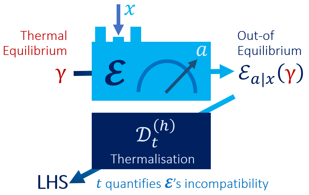
Figure 1: Schematic interpretation of the framework. We aim to quantify the incompatibility of instruments in a thermodynamic setting. The idea is to analyse the instrument’s ability to drive the system out of thermal equilibrium (and thus potentially generate quantum signature via incompatibility), and then check how long it takes to use thermalisation to remove the quantum signature.

Incompatibility signature can survive thermalisation

After introducing the figure-of-merit, the first thing to check is that it is non-trivial; namely, it can indeed detect instrument incompatibility. Physically, this amounts to answering the question: can incompatibility sigunature survive thermalisation? It turns out that $t_{\rm min}^{(h)}$ can be related to a steering measure that we call (logarithmic) thermalisation steering robustness subject to $\gamma$, denoted by ${\rm SR}_{\gamma}$. Formally, for a state assemblage ${\bm{\sigma}}=\{\sigma_{a|x}\}_{a,x}$, we define $2^{{\rm SR}_{\gamma}({\bm{\sigma}})}$ to be

$$\min\left\{\lambda\geq 1\,\middle|\,\left\{\frac{\sigma_{a|x}+(\lambda-1){\rm tr}(\sigma_{a|x})\gamma}{\lambda}\right\}_{a,x}\in{\bf LHS}\right\}.$$ (6)

It is a direct computation to verify that it can quantify steering, as ${\rm SR}_{\gamma}({\bm{\sigma}})=0$ if and only if ${\bm{\sigma}}\in{\bf LHS}$, and it is non-increasing under certain allowed operations of steering [34]. Moreover, by writing $\mathbfcal{E}(\gamma)\coloneqq\{\mathcal{E}_{a,x}(\gamma)\}_{a,x}$, we have

$$t_{\rm min}^{(h)}(\mathbfcal{E})=h^{-1}\left(2^{-{\rm SR}_{\gamma}[\mathbfcal{E}(\gamma)]}\right).$$ (7)

We then conclude that

Observation 1.

As long as $\mathbfcal{E}(\gamma)\notin{\bf LHS}$, the signature of instrument incompatibility can be seen within a non-vanishing time window $0\leq t<t_{\rm min}^{(h)}(\mathbfcal{E})$.

Hence, our figure-of-merit is indeed non-trivial, as it can indeed certify the signature of instrument incompatibility. In fact, one can further use $t_{\rm min}^{(h)}$ to quantify incompatible instruments, as we detail later.

As an example, consider $h(t)=h_{\rm pt}(t)\coloneqq e^{-t/t_{0}},$ where $t_{0}$ is the thermalisation time scale. This is called partial thermalistaion, achievable by collision models [35] and Davies dynamical semigroup [36], which is a simple yet practical model for thermalisation processes (see, e.g., Refs. [37, 27, 38] for its applications). Using this, Eq. (7) becomes

$$t_{\rm min}^{\left(h_{\rm pt}\right)}(\mathbfcal{E})/t_{0}\ln 2={\rm SR}_{\gamma}[\mathbfcal{E}(\gamma)].$$ (8)

Hence, under the partial thermalisation model, ${\rm SR}_{\gamma}$ is the thermalisation time in the unit $t_{0}\ln 2$.

Finally, we remark that Eq. (6) is in fact a semi-definite programming (SDP) [39, 40]. Hence, it is a numerically feasible measure that can be efficiently computed. We refer the reader to Supplemental Material I for its dual problem [see Eq. (17)], and we focus on physical interpretation in the main text.

Deterministic allowed operations and quantifying instrument incompatibility by thermalisation

Clearly, due to the thermodynamic constraints of our framework, not every operation is allowed. In fact, in our setting, any deterministic allowed operation takes the following form: it is a mapping $\mathbfcal{E}\mapsto\mathbb{F}(\mathbfcal{E})$ such that $\mathbb{F}(\mathbfcal{E})_{a|x}\coloneqq\sum_{b,y}P^{\prime}(a|xyb)P(y|x)\mathcal{D}\circ\mathcal{E}_{b|y}\circ\mathcal{P},$ where both $\mathcal{D},\mathcal{P}$ are Gibbs-preserving channels [i.e., $\mathcal{D}(\gamma)=\gamma=\mathcal{P}(\gamma)$]. Physically, we allow operations that keep thermal equilibrium untouched, including classical pre- and post-processing, and quantum pre- and post-measurement channels that are Gibbs-preserving .

The deterministic allowed operations clearly cannot generate instrument incompatibility from a compatible one — when $\mathbfcal{E}$ is compatible, one can check that $\mathbb{F}(\mathbfcal{E})$ must also be compatible. Using the resource-theoretic approach, we prove the following result:

Result 2.

$t_{\rm min}^{(h)}$ is an instrument incompatibility monotone; that is, for every instrument $\mathbfcal{E}$ in the current framework, $t_{\rm min}^{(h)}(\mathbfcal{E})=0$ if $\mathbfcal{E}$ is compatible. Also, $t_{\rm min}^{(h)}[\mathbb{F}(\mathbfcal{E})]\leq t_{\rm min}^{(h)}(\mathbfcal{E})$ for every deterministic allowed operations $\mathbb{F}$.

We detail the proof in Supplemental Material II. Hence, with the notion of deterministic allowed operations, we can quantify incompatible instruments thermodynamically.

Stochastic allowed operations and their physical implications

So far, we solely discuss deterministic allowed operations, while it is also important to study the case when the operations are probabilistic, or, say, stochastic [42, 43, 44, 45, 46, 47]. This is particularly important in the recent studies of stochastic distillation of steering and incompatibility [45, 46, 47]. Following the recent study, in this work, we focus on a special type of stochastic operations that is termed ${\rm LF_{1}}$, which are filters consisting of a single Kraus operator. Despite its simple form, it can already achieve optimal performance in, e.g., stochastic steering distillation [45, 46, 47]. This thus motivates us to focus on this type of filters for its physical relevance. Hence, the stochastic allowed operation that we consider here are ${\rm LF_{1}}$ operations $K(\cdot)K^{\dagger}$ satisfying

$$K\gamma K^{\dagger}/p_{\gamma}=\gamma,$$ (9)

where $p_{\gamma}={\rm tr}(K\gamma K^{\dagger})$ is the success probability of this filter operation. This can be understood as ${\rm LF_{1}}$ filters with an additional thermodynamic condition — they cannot drive thermal equilibrium out of equilibrium. With this notion in hand, we have the following no-go result:

Result 3.

In our current framework, no stochastic allowed operation can increase $t_{\rm min}^{(h)}$.

See Supplemental Material III for the proof. Hence, the ability to drive the system out of thermal equilibrium is necessary to increase $t_{\rm min}^{(h)}$ even stochastically. This also means that $t_{\rm min}^{(h)}$ is monotonic under stochastic allowed operations. Interestingly, as $t_{\rm min}^{(h)}$ can also be viewed as a steering measure, this no-go result also suggests that we cannot stochastically distil steering in the current thermodynamic framework.

Incompatibility signature always vanishes at finite time when system thermalises

We have discussed thermalisaion achieved by Markovian evolutions. Here comes a general question addressing the fundamental structure of general evolution, no matter whether Markovian or not: If an evolution thermalises a quantum system, can incompatibility signature survive at every finite time instant? More precisely, an evolution is defined to be a one-parameter family of channels $\mathfrak{E}\coloneqq\{\mathcal{N}_{t}\}_{t=0}^{\infty}$, where the parameter $t$ indicates the time instant. Physically, it means that when the initial state at $t=0$ is $\rho$, then at time instant $t$ the state evolves to $\mathcal{N}_{t}(\rho)$. We then say the evolution $\mathfrak{E}$ thermalises the given system to the thermal state $\gamma$ if $\lim_{t\to\infty}\left\|\mathcal{N}_{t}(\cdot)-\gamma{\rm tr}(\cdot)\right\|_{\diamond}=0.$ Note that we choose the diamond norm purely for convenience. Other distance measures should also work without changing the physics. Note that this definition implies that $\lim_{t\to\infty}\left\|\mathcal{N}_{t}(\rho)-\gamma\right\|_{\diamond}=0$ for every initial state $\rho$. One can directly see that the thermalisation models that we consider in Eq. (4) form a strict subset of such evolutions. In fact, here we only demand the minimal assumptions about thermalisation, and there exist lots of non-Markovian evolutions that can also thermalise a system. Notably, this definition also works if we simply consider $\mathcal{N}_{t}$’s as positive linear maps — that is, they can also be non-physical. A natural question is whether one can make use of these additional resources to somehow protect the quantum signature of incompatiblity and steering. This is, surprisingly, impossible, as we can prove the following no-go result:

Result 4.

Let ${\bm{\sigma}}$ be a state assemblage with reduced state $\gamma$. Suppose that $\gamma$ is full-rank, and $p_{a|x}\coloneqq{\rm tr}(\sigma_{a|x})>0$ for every $a,x$. Then $\{p_{a|x}\gamma\}_{a,x}$ is in the relative interior of ${\bf LHS}$. Moreover, for an evolution $\mathfrak{E}$ thermalising the system to $\gamma$, there must exists a finite $t_{*}$ such that $\mathcal{N}_{t}({\bm{\sigma}})\in{\bf LHS}$ $\forall\;t>t_{*}.$ Namely, signatures of incompatibility and steering must vanish at finite time.

We detail the proof in Supplemental Material IV. Hence, even with non-Markovianity or non-physical linear maps, it is impossible to keep the signature of steering and incompatibility forever. In fact, our finding even suggests that thermalisation not only removes the quantum signature but also wipes out the effects of non-physical maps.

Instrument incompatibility and steering provide advantages in work extraction tasks

After knowing how to use thermalisation processes to quantify incompatibility, a natural question is whether any other thermodynamic task can also be used in quantification. Here, we further investigate the operational interpretation of ${\rm SR}_{\gamma}$ in a work extraction tasks formulated as follows (see Ref. [48] for detail). Consider a finite-dimensional quantum system with Hamiltonian $H$ and background temperature $T$. When this system is in a state $\rho$, one can extract the following optimal amount of work from it (see, e.g., Ref. [49]): $W_{{\rm ext}}(\rho,H)=(k_{B}T\ln 2)D\left(\rho\,\|\,\gamma\right),$ where $D(\rho\,\|\,\sigma)\coloneqq{\rm tr}\left[\rho\left(\log_{2}\rho-\log_{2}\sigma\right)\right]$ is the quantum relative entropy, and $\gamma$ is again the thermal state associated with $H$ and $T$. A special case is when there is no energy gap; i.e., $H=0$. This gives the following work value describing the optimal work that can be extracted from the information content of $\rho$: $W_{{\rm inf}}(\rho)\coloneqq W_{{\rm ext}}(\rho,H=0)=(k_{B}T\ln 2)D\left(\rho\,\|\,\mathbb{I}/d\right).$ Following Ref. [48], we then consider the following deficit-type figure-of-merit that is inspired by Ref. [30] (see also the first arXiv version of Ref. [28]):

$$\Delta(\rho,H)\coloneqq W_{{\rm ext}}(\rho,H)-W_{{\rm inf}}(\rho),$$ (10)

which characterises the difference between $\rho$’s performances in two types of work extraction scenarios; namely, one is subject to the given Hamiltonian $H$, and one is solely addressing the information content of $\rho$. $\Delta$ is thus the ‘score’ of the given state $\rho$ in this game-type setting — a Hamiltonian $H$ defines a specific ‘game’, a state $\rho$ is player’s strategy, and $\Delta$ is the score, quantifying the performance. See Ref. [48] for details.

Now, we apply a similar idea to state assemblages. For a state assemblage ${\bm{\sigma}}$ describing states $\hat{\sigma}_{a|x}\coloneqq\sigma_{a|x}/p_{a|x}$ prepared with probabilities $p_{a|x}={\rm tr}(\sigma_{a|x})$, we consider the following figure-of-merit with Hamiltonians ${\bf H}=\{H_{a|x}\}_{a,x}$:

$$\overline{\Delta}_{\gamma}({\bm{\sigma}},{\bf H})\coloneqq\sum_{a,x}p_{a|x}\left[\Delta(\hat{\sigma}_{a|x},H_{a|x})-\Delta(\gamma,H_{a|x})\right]$$ (11)

In Supplemental Material V, we show that this is the figure-of-merit relevant to the quantification:

Result 5.

Let ${\bm{\sigma}}$ be a state assemblage with reduced state $\rho_{\bm{\sigma}}=\gamma$ and $\mathcal{H}_{+}({\bm{\sigma}})\coloneqq\left\{{\bf H}\;\middle|\;\overline{\Delta}_{\gamma}({\bm{\sigma}},{\bf H})\geq 1\right\}.$ Then we have

$$2^{{\rm SR}_{\gamma}({\bm{\sigma}})}=\max_{{\bf H}\in\mathbfcal{H}_{+}({\bm{\sigma}})}\frac{\overline{\Delta}_{\gamma}({\bm{\sigma}},{\bf H})}{\max_{{\bm{\tau}}\in{\bf LHS}}\overline{\Delta}_{\gamma}({\bm{\tau}},{\bf H})}.$$ (12)

This result provides an alternative thermodynamic interpretation of ${\rm SR}_{\gamma}$ — it has an operational meaning in work extraction tasks quantified by the figure-of-merit $\overline{\Delta}_{\gamma}$. This finding also builds the link between the thermalisation process [quantified by $t_{\rm min}^{(h)}$ as defined in Eq. (5)] and the work extraction task (quantified by $\Delta_{\gamma}$). Finally, it is worth mentioning that, by using the dual SDP of Eq. (6) [see Eq. (17)], one can prove a similar thermodynamic interpretation as follows (see Supplemental Material V):

Corollary 6.

Let ${\bm{\sigma}}$ be a state assemblage with reduced state $\rho_{\bm{\sigma}}=\gamma$. Then ${\rm SR}_{\gamma}({\bm{\sigma}})>0$ if and only if there is ${\bf H}$ such that $\overline{\Delta}_{\gamma}({\bm{\sigma}},{\bf H})>\max_{{\bm{\tau}}\in{\bf LHS}}\overline{\Delta}_{\gamma}({\bm{\tau}},{\bf H}).$ Moreover, running SDP can explicitly find this ${\bf H}$.

Informational non-equilibrium and measurement incompatibility

In the special case $\gamma=\mathbb{I}/d$, which is when we turn off the energy gaps in Hamiltonian, we enter the regime of the so-called informational non-equilibrium [50]. With this setting, the average Gibbs-preserving condition Eq. (3) becomes $\sum_{a}\mathcal{E}_{a|x}(\mathbb{I})=\mathbb{I}$; namely, the average channel is unital. This means that $\mathbfcal{E}(\mathbb{I}/d)$ can be equivalently viewed as measurement assemblage by simply considering $\mathbfcal{E}(\mathbb{I})$. That is, for each $x$, the set $\{\mathcal{E}_{a|x}(\mathbb{I})\}_{a}$ is a positive operator-valued measure (POVM) [51], meaning that $\sum_{a}\mathcal{E}_{a|x}(\mathbb{I})=\mathbb{I}$ for every $x$ and $\mathcal{E}_{a|x}(\mathbb{I})\geq 0$ for every $a,x$. Then we have $t_{\rm min}^{(h)}(\mathbfcal{E})=\min\left\{t\geq 0\,\middle|\,\left\{\mathcal{D}_{t}^{(h)}\left[\mathcal{E}_{a|x}(\mathbb{I})\right]\right\}_{a,x}\in{\bf JM}\right\},$ where ${\bf JM}$ stands for jointly measurable measurement assemblages, which are those satisfying $M_{a|x}=\sum_{\lambda}P(a|x,\lambda)G_{\lambda}$ for some conditional probability distribution $\{P(a|x,\lambda)\}_{a,x,\lambda}$ and a single POVM $\{G_{\lambda}\}_{\lambda}$. Measurement assemblages that are not jointly measurable are said to be incompatible. Hence, in the regime of informational non-equilibrium, our result naturally provides a thermodynamic approach to quantify measurement incompatibility.

Bridging steering distillation and thermalisation time of instrument incompatibility

To better interpret the physics in the regime of $\gamma=\mathbb{I}/d$, let us now consider the partial thermalisation model; i.e., $h(t)=h_{\rm pt}(t)\coloneqq e^{-t/t_{0}}$. For convenience, let us denote the (dimensionless) normalised time scale as $T_{\rm min}^{\rm(pt)}(\mathbfcal{E})\coloneqq t_{\rm min}^{\left(h_{\rm pt}\right)}(\mathbfcal{E})/t_{0}\ln 2.$ Now, suppose ${\bm{\sigma}}$ is a state assemblage with a full-rank reduced state $\rho_{\bm{\sigma}}$. Then its steering equivalent observable (SEO) is a measurement assemblage ${\bf B}^{({\bm{\sigma}})}$ defined by [52, 53] $B_{a|x}^{({\bm{\sigma}})}\coloneqq\sqrt{\rho_{\bm{\sigma}}}\sigma_{a|x}\sqrt{\rho_{\bm{\sigma}}}\,\forall\;a,x.$ SEO is a key tool in the study of steering and measurement incompatibility [52, 53, 45, 46, 47]. In fact, by using the notion of SEO, we can uncover a trade-off relation between thermalisation time and distillable steering. To measure the amount of distillable steering in a general sense, let us now consider the generalised (logarithmic) steering robustness [54, 55] as defined by ${\rm SR}({\bm{\sigma}})\coloneqq\log_{2}\min\left\{\lambda\geq 1\;\middle|\;\sigma_{a|x}\leq\lambda\tau_{a|x},{\bm{\tau}}\in{\bf LHS}\right\}.$ Then we have the following result:

Result 7.

Let ${\bm{\sigma}}$ be a state assemblage with a full-rank reduced state. Then, in the case of $\gamma=\mathbb{I}/d$, we have $\min\left\{T_{\rm min}^{\rm(pt)}(\mathbfcal{E})\;\middle|\;\mathbfcal{E}(\mathbb{I})={\bf B}^{({\bm{\sigma}})}\right\}\geq\max\left\{{\rm SR}({\bm{\tau}})\;\middle|\;{\bm{\sigma}}\xrightarrow{\rm LF_{1}}{\bm{\tau}}\right\}.$

We give the proof in Supplemental Material VI. In the above inequality, the minimisation is taken over all $\mathbfcal{E}$ that can reproduce ${\bm{\sigma}}$’s SEO by inputting $\mathbb{I}$; namely, $\sqrt{\rho_{\bm{\sigma}}}\mathcal{E}_{a|x}(\mathbb{I})\sqrt{\rho_{\bm{\sigma}}}=\sigma_{a|x}$ for every $a,x$, where $\rho_{\bm{\sigma}}$ is the reduced state of ${\bm{\sigma}}$. On the other hand, the maximisation is taken over all state assemblages that can be reached by ${\bm{\sigma}}$ via any ${\rm LF_{1}}$ filter operation.

Hence, interestingly, the thermalisation time scale $T_{\rm min}^{\rm(pt)}$ acts as a fundamental limitation of the general stochastic steering distillation through ${\rm LF_{1}}$ filters. Note that ${\rm LF_{1}}$ filters has been shown to be sufficiently general, since no general filter can outperform them in steering distillation; see Refs. [46, 47] for details. Result 7 thus implies that the shortest possible time to erase the incompatible signature in the current thermalisation setup upper bounds the highest general distillable steerability.

One can also interpret Result 7 in a different way. Suppose we know that certain amount of steerability can be stochastically distilled from the state assemblage $\mathbfcal{E}(\mathbb{I}/d)$, say, $\max\left\{{\rm SR}({\bm{\tau}})\;\middle|\;\mathbfcal{E}(\mathbb{I}/d)\xrightarrow{\rm LF_{1}}{\bm{\tau}}\right\}\geq\delta$. Then we can directly conclude that $\mathbfcal{E}$’s incompatible signature can survive partial thermalisation (toward $\mathbb{I}/d$) for at least $t=\delta\times t_{0}\ln 2$.

To sum, in a thermodynamic way, Result 7 poses a fundamental limitation on the optimal distillable steerability under ${\rm LF_{1}}$ filters. It also uncovers the quantitative link between the thermalisation time scale needed to remove signatures of instrument incompatibility and the optimal stochastic distillation of quantum steering.

Discussions

In this work, we introduce a thermodynamic framework to quantify incompatible instruments. The quantification is achieved by a special type of steering robustness measure, which has clear thermodynamic meanings in thermalisation and work extraction tasks. We further analyse operations that cannot increase this steering measure, uncovering a series of no-go results and fundamental limitations related to stochastic steering distillation.

Many questions remain open. First, it is worth mentioning that we consider filter operations subject to a specific physical constraint. A more general question is how to consider stochastic allowed operations in a general resource theoretic setting. We leave this to our follow-up projects, as this is beyond the scope of this work. Second, we introduce the first thermodynamic way to quantify instrument incompatibility. It is then interesting to know how to make the thermodynamic tasks more feasible experimentally in practical setups so that such a theoretical quantification can really be done in labs. Third, a natural question is whether other types of steering measures, such as steerable weight, can give us similar thermodynamic meanings in work extraction tasks once we impose suitable thermodynamic constraints. Finally, as we focus on the so-called traditional incompatibility of instruments (see, e.g., Ref. [17]), it will be valuable to study other types of incompatibility [18, 19, 20, 21, 22, 17, 23, 24, 25, 7, 8, 14] in a similar thermodynamic context. We leave this for future investigation.

I SUPPLEMENTAL MATERIAL

I.1 Supplemental Material I: ${\rm SR}_{\gamma}$ as an SDP

First of all, for an arbitrarily given ${\bm{\tau}}\in{\bf LHS}$, we can write, for every $a,x$, $\tau_{a|x}=\sum_{i=1}^{|{\bf i}|}q_{i}D(a|x,i)\rho_{i},$ which sums over all possible deterministic probability distributions $D(a|x,i)$, where each of them assigns exactly one output value $a$ for each input $x$ [4, 5]. In other words, each $D(a|x,i)$ is a deterministic mapping from $x=0,1,...,|{\bf x}|-1$ to $a=0,1,...,|{\bf a}|-1$, and there are $|{\bf i}|\coloneqq|{\bf a}|^{|{\bf x}|}$ many of them. By defining $\eta_{i}=q_{i}\rho_{i}$, we obtain a simple useful fact [4, 5]:

Fact 8.

Every ${\bm{\tau}}\in{\bf LHS}$ can be expressed by $\tau_{a|x}=\sum_{i=1}^{|{\bf i}|}D(a|x,i)\eta_{i}$ with $\eta_{i}\geq 0$ and $\sum_{i=1}^{|{\bf i}|}{\rm tr}(\eta_{i})=1$.

Using the above fact and Eq. (6), we can write $2^{-{\rm SR}_{\gamma}({\bm{\sigma}})}$ into the following form [recall that $p_{a|x}={\rm tr}(\sigma_{a|x})$; also, from now on, $\sum_{i}$ is the abbreviation of $\sum_{i=1}^{|{\bf i}|}$]:

$$\begin{split}\max_{\{\eta_{i}\}_{i},q}\quad&q\\ {\rm s.t.}\quad&0\leq q\leq 1;\;\;\eta_{i}\geq 0\;\forall\,i;\\ &\sum_{i}D(a|x,i)\eta_{i}+q(\gamma p_{a|x}-\sigma_{a|x})=\gamma p_{a|x}\;\forall\,a,x.\end{split}$$ (13)

Note that the constraint $\sum_{i}{\rm tr}(\eta_{i})=1$ is already guaranteed by taking trace and summing over $a$ of the constraint $\sum_{i}D(a|x,i)\eta_{i}+q(\gamma p_{a|x}-\sigma_{a|x})=\gamma p_{a|x}$. Now, define ${\bf V}\coloneqq\left(\bigoplus_{i}\eta_{i}\right)\oplus q,$ ${\bf B}\coloneqq\bigoplus_{a,x}\left(\gamma p_{a|x}\right),$ and $\Phi({\bf V})\coloneqq\bigoplus_{a,x}\left[\sum_{i}D(a|x,i)\eta_{i}+q(\gamma p_{a|x}-\sigma_{a|x})\right],$ where $\Phi$ is a hermitian-preserving linear map. Then we have

$$\begin{split}2^{-{\rm SR}_{\gamma}({\bm{\sigma}})}=\max_{{\bf V}}\quad&q\\ {\rm s.t.}\quad&\Phi({\bf V})={\bf B};\;\;q\leq 1;\;\;{\bf V}\geq 0.\end{split}$$ (14)

This is in the standard form of the primal problem of SDP, whose dual problem is given by [39, 40]

$$\begin{split}\min_{{\bf H},\omega}\quad&\sum_{a,x}{\rm tr}\left(H_{a|x}\gamma\right)p_{a|x}+\omega\\ {\rm s.t.}\quad&H_{a|x}=H_{a|x}^{\dagger}\;\forall\,a,x;\;\;\omega\geq 0;\\ &\Phi^{\dagger}(H)+\left(\bigoplus_{i}0\right)\oplus\omega\geq\left(\bigoplus_{i}0\right)\oplus 1,\end{split}$$ (15)

where ${\bf H}=\bigoplus_{a,x}H_{a|x}$. Now, we have

$$\sum_{a,x}{\rm tr}\left(H_{a|x},\Phi({\bf V})_{a|x}\right)=\sum_{i}{\rm tr}\left[\sum_{a,x}H_{a|x}D(a|x,i)\eta_{i}\right]$$

$$\quad\quad\quad+{\rm tr}\left[\sum_{a,x}H_{a|x}(\gamma p_{a|x}-\sigma_{a|x})\right]\times q.$$ (16)

Hence, using the definition of inner product, we conclude that $\Phi^{\dagger}({\bf H})=\left[\bigoplus_{i}\left(\sum_{a,x}H_{a|x}D(a|x,i)\right)\right]\oplus{\rm tr}\left[\sum_{a,x}H_{a|x}(\gamma p_{a|x}-\sigma_{a|x})\right],$ and we obtain the dual form of $2^{-{\rm SR}_{\gamma}({\bm{\sigma}})}$ as follows:

$$\begin{split}\min_{{\bf H},\omega}\quad&\sum_{a,x}{\rm tr}(H_{a|x}\gamma)p_{a|x}+\omega\\ {\rm s.t.}\quad&H_{a|x}=H_{a|x}^{\dagger}\;\forall\,a,x;\;\;\omega\geq 0;\\ &\sum_{a,x}D(a|x,i)H_{a|x}\geq 0\;\forall\,i;\\ &\sum_{a,x}{\rm tr}(H_{a|x}\gamma)p_{a|x}+\omega\geq\sum_{a,x}{\rm tr}(H_{a|x}\sigma_{a|x})+1.\end{split}$$ (17)

Note that this is equal to $2^{-{\rm SR}_{\gamma}({\bm{\sigma}})}$ since the strong duality holds [39] — this can be checked by noting that the primal problem is finite and feasible (e.g., by simply considering $q=0$), and the dual problem is strictly feasible; namely, by choosing $\omega>1$ and $H_{a|x}=\mathbb{I}$ for every $a,x$, one can achieve $\sum_{a,x}D(a|x,i)H_{a|x}>0\;\forall\,i$ and $\sum_{a,x}{\rm tr}(H_{a|x}\gamma)p_{a|x}+\omega>\sum_{a,x}{\rm tr}(H_{a|x}\sigma_{a|x})+1$ (see, e.g., Theorem 1.18 in Ref. [39]).

I.2 Supplemental Material II: Proof of Result 2

Proof.

First, if $\mathbfcal{E}$ is compatible, one can directly conclude that $t_{\rm min}^{(h)}(\mathbfcal{E})=0$ by Eq. (7). Hence, it suffices to show the non-increasing property under deterministic allowed operations. Note that the decomposition given in the definition of ${\rm SR}_{\gamma}[\mathbb{F}(\mathbfcal{E})(\gamma)]$ [i.e., Eq. (6)] can be re-written as (in what follows, we define $q=1/\lambda$)

$$q\mathbb{F}(\mathbfcal{E})_{a|x}(\gamma)+(1-q){\rm tr}[\mathbb{F}(\mathbfcal{E})_{a|x}(\gamma)]\gamma$$

$$=q\sum_{b,y}P^{\prime}(a|xyb)P(y|x)\mathcal{D}\circ\mathcal{E}_{b|y}\circ\mathcal{P}(\gamma)$$

$$\quad+(1-q)\sum_{b,y}P^{\prime}(a|xyb)P(y|x){\rm tr}\left[\mathcal{D}\circ\mathcal{E}_{b|y}\circ\mathcal{P}(\gamma)\right]\gamma$$

$$=\sum_{b,y}P^{\prime}(a|xyb)P(y|x)\mathcal{D}\biggl{(}q\mathcal{E}_{b|y}(\gamma)+(1-q){\rm tr}\left[\mathcal{E}_{b|y}(\gamma)\right]\gamma\biggr{)},$$ (18)

where we have used the trace-preserving as well as Gibbs-preserving properties of $\mathcal{D},\mathcal{P}$. Consequently, $2^{-{\rm SR}_{\gamma}[\mathbb{F}(\mathbfcal{E})(\gamma)]}$ can be expressed as

$$\begin{split}\max_{{\bf V}}\quad&q\\ {\rm s.t.}\quad&0\leq q\leq 1;\;\;{\bm{\omega}}\in{\bf LHS};\;\;\forall a,x:\\ &\omega_{a|x}=\sum_{b,y}P^{\prime}(a|xyb)P(y|x)\\ &\quad\quad\;\times\mathcal{D}\biggl{(}q\mathcal{E}_{b|y}(\gamma)+(1-q){\rm tr}\left[\mathcal{E}_{b|y}(\gamma)\right]\gamma\biggr{)}.\end{split}$$ (19)

Note that $\left\{\sum_{b,y}P^{\prime}(a|xyb)P(y|x)\mathcal{D}(\tau_{b|y})\right\}_{a,x}\in{\bf LHS}$ if ${\bm{\tau}}\in{\bf LHS}$, since it is a free operation of steering [34]. Hence, $2^{-{\rm SR}_{\gamma}[\mathbb{F}(\mathbfcal{E})(\gamma)]}$ is lower bounded by

$$\begin{split}\max_{{\bf V}}\quad&q\\ {\rm s.t.}\quad&0\leq q\leq 1;\;\;{\bm{\tau}}\in{\bf LHS};\\ &\tau_{a|x}=q\mathcal{E}_{a|x}(\gamma)+(1-q){\rm tr}\left[\mathcal{E}_{a|x}(\gamma)\right]\gamma\,\forall a,x,\end{split}$$ (20)

which is exactly $2^{-{\rm SR}_{\gamma}[\mathbfcal{E}(\gamma)]}$. Finally, by using Eq. (7) and the fact that the function $h^{-1}(y):[0,1]\to\mathbb{R}$ is again non-increasing, we conclude that

$$t_{\rm min}^{(h)}[\mathbb{F}(\mathbfcal{E})] =h^{-1}\left(2^{-{\rm SR}_{\gamma}[\mathbb{F}(\mathbfcal{E})(\gamma)]}\right)$$

$$\leq h^{-1}\left(2^{-{\rm SR}_{\gamma}[\mathbfcal{E}(\gamma)]}\right)=t_{\rm min}^{(h)}(\mathbfcal{E}).$$ (21)

The proof is thus completed. ∎

I.3 Supplemental Material III: Proof of Result 3

Proof.

Suppose that there exists an allowed stochastic operation, which is an ${\rm LF_{1}}$ filter $K$, achieving $\sigma_{a|x}\mapsto\omega_{a|x}=K\sigma_{a|x}K^{\dagger}/p_{\gamma},$ where, again, $p_{\gamma}={\rm tr}\left(K\gamma K^{\dagger}\right)$. Using the recent results [45, 47], this implies that there exists a unitary operator $U$ and a state $\eta$ with ${\rm supp}(\eta)\subseteq{\rm supp}(\gamma)$ achieving $\omega_{a|x}=\sqrt{\eta}U\sqrt{\gamma}^{\;-1}\sigma_{a|x}\sqrt{\gamma}^{\;-1}U^{\dagger}\sqrt{\eta}\;\forall\;a,x.$ One can directly check that the reduced state of ${\bm{\omega}}$ is $\eta=U\gamma U^{\dagger}.$ Now, since this ${\rm LF_{1}}$ filter is a stochastic allowed operation, Eq. (9) implies that the reduced state of ${\bm{\omega}}$ must also be the given thermal state $\gamma$. Namely, we must have $\eta=U\gamma U^{\dagger}=\gamma.$ In other words, the unitary must conserve the energy due to $\gamma U=U\gamma$, and the whole filter operation takes the form

$$\omega_{a|x}=\sqrt{\gamma}U\sqrt{\gamma}^{\;-1}\sigma_{a|x}\sqrt{\gamma}^{\;-1}U^{\dagger}\sqrt{\gamma}=U\sigma_{a|x}U^{\dagger}\;\forall\;a,x.$$ (22)

This means that, after the given ${\rm LF_{1}}$ filter operation,

$$2^{-{\rm SR}_{\gamma}({\bm{\omega}})}=\max\left\{0\leq q\leq 1\,\middle|\,q\omega_{a|x}+(1-q){\rm tr}(\omega_{a|x})\gamma\in{\bf LHS}\right\}$$

$$=\max\left\{0\leq q\leq 1\,\middle|\,U\left[q\sigma_{a|x}+(1-q){\rm tr}(\omega_{a|x})\gamma\right]U^{\dagger}\in{\bf LHS}\right\}$$

$$=\max\left\{0\leq q\leq 1\,\middle|\,q\sigma_{a|x}+(1-q){\rm tr}(\sigma_{a|x})\gamma\in{\bf LHS}\right\}$$

$$=2^{-{\rm SR}_{\gamma}({\bm{\sigma}})},$$ (23)

where we have used the commutation relation $\gamma U=U\gamma$, ${\rm tr}(U\sigma_{a|x}U^{\dagger})={\rm tr}(\sigma_{a|x})$, and the fact that $U{\bm{\tau}}U^{\dagger}\in{\bf LHS}$ if and only if ${\bm{\tau}}\in{\bf LHS}$. Hence, from here we conclude that:

No stochastic allowed operation can change ${\rm SR}_{\gamma}$.

Consequently, it is impossible to increase $t_{\rm min}^{(h)}$. ∎

I.4 Supplemental Material IV: Lemmas and Proofs related to Result 4

I.4.1 Relative interior of ${\bf LHS}$

The relative interior of ${\bf LHS}$ can be written by [56]

$${\rm relint}({\bf LHS})\coloneqq$$

$$\left\{{\bm{\tau}}\in{\bf LHS}\;\middle|\;\exists\;\epsilon>0\;\text{s.t.}\;\mathcal{B}({\bm{\tau}};\epsilon)\cap{\rm aff}({\bf LHS})\subseteq{\bf LHS}\right\},$$ (24)

where $\mathcal{B}({\bm{\tau}};\epsilon)\coloneqq\left\{\{A_{a|x}\}_{a,x}\;\middle|\;\sum_{a,x}\left\|A_{a|x}-\tau_{a|x}\right\|_{1}<\epsilon\right\}$ is an open ball centring at ${\bm{\tau}}$ with radius $\epsilon$ (here, $A_{a|x}$ are some hermitian operators, and we use the metric $d({\bf A},{\bf B})\coloneqq\sum_{a,x}\left\|A_{a|x}-B_{a|x}\right\|_{1}$ defined in Ref. [28], which induces a metric topology), and

$${\rm aff}({\bf LHS})\coloneqq$$

$$\left\{\sum_{k=1}^{K}a_{k}{\bm{\tau}}_{k}\;\middle|\;K\in\mathbb{N},a_{k}\in\mathbb{R},{\bm{\tau}}_{k}\in{\bf LHS},\sum_{k=1}^{K}a_{k}=1\right\}$$ (25)

is the affine hull of the set ${\bf LHS}$. Then we have the following lemma:

Lemma 9.

Let ${\bm{\sigma}}$ be a state assemblage with reduced state $\gamma$. Suppose that $\gamma$ is full-rank, and $p_{a|x}\coloneqq{\rm tr}(\sigma_{a|x})>0$ for every $a,x$. Then $\{p_{a|x}\gamma\}_{a,x}\in{\rm relint}({\bf LHS}).$

Proof.

By Fact 8, every ${\bm{\kappa}}\in{\bf LHS}$ can be expressed by $\kappa_{a|x}=\sum_{i=1}^{|{\bf i}|}D(a|x,i)\eta_{i}\;\forall\,a,x$ with some $\eta_{i}\geq 0$ satisfying $\sum_{i}{\rm tr}(\eta_{i})=1$, and there are $|{\bf i}|\coloneqq|{\bf a}|^{|{\bf x}|}$ many of deterministic probability distributions $D(a|x,i)$’s. Now, we write

$$p_{a|x}=(1-\epsilon)\widetilde{p}_{a|x}+\epsilon/|{\bf a}|,$$ (26)

where $\widetilde{p}_{a|x}\coloneq(p_{a|x}-\epsilon/|{\bf a}|)/(1-\epsilon)$ is a valid probability distribution with a small enough $\epsilon>0$ since we have $p_{a|x}>0$ $\forall\;a,x$. Now, for $0<s<1$, we have

$$p_{a|x}\gamma-s\kappa_{a|x}=(1-\epsilon)\widetilde{p}_{a|x}\gamma+\epsilon\gamma/|{\bf a}|-s\sum_{i=1}^{|{\bf i}|}D(a|x,i)\eta_{i}$$

$$=(1-\epsilon)\widetilde{p}_{a|x}\gamma+\sum_{i=1}^{|{\bf i}|}D(a|x,i)\left(\epsilon\gamma/|{\bf i}|-s\eta_{i}\right),$$ (27)

where, in the second line, we use the relation $\sum_{i=1}^{|{\bf i}|}D(a|x,i)=|{\bf a}|^{|{\bf x}|-1}=|{\bf i}|/|{\bf a}|$ for every $a,x$ (i.e., for the given input $x$, the deterministic outcome $a$ has been assigned; for each other input, we have $|{\bf a}|$ many possible outcomes). Since $\gamma$ is full-rank, we have $\gamma\geq\mu_{\rm min}(\gamma)\mathbb{I}$, where $\mu_{\rm min}(\gamma)>0$ is the smallest eigenvalue of $\gamma$. Then we choose

$$0<s<\min\left\{\epsilon;\frac{\epsilon\mu_{\rm min}(\gamma)}{|{\bf i}|\max_{j}\left\|\eta_{j}\right\|_{\infty}}\right\}.$$ (28)

Note that $\epsilon\mu_{\rm min}(\gamma)/|{\bf i}|\max_{j}\left\|\eta_{j}\right\|_{\infty}>0$ and this interval is non-vanishing. For these value $s$ and every $i$, we obtain

$$s\eta_{i}\leq s\max_{j}\left\|\eta_{j}\right\|_{\infty}\mathbb{I}\leq\epsilon\mu_{\rm min}(\gamma)\mathbb{I}/|{\bf i}|\leq\epsilon\gamma/|{\bf i}|.$$ (29)

This means that $W_{i}\coloneqq(\epsilon\gamma/|{\bf i}|-s\eta_{i})/(\epsilon-s)\geq 0$ for every $i$ (note that in the interval that we set, we have $\epsilon-s>0$) and $\sum_{i=1}^{|{\bf i}|}{\rm tr}(W_{i})=1$. By Fact 8, we conclude that the state assemblage $\omega_{a|x}\coloneqq\sum_{i=1}^{|{\bf i}|}D(a|x,i)W_{i}$ is in ${\bf LHS}$. Substituting everything back to Eq. (I.4.1), we obtain

$$\frac{p_{a|x}\gamma-s\kappa_{a|x}}{1-s}=\left(\frac{1-\epsilon}{1-s}\right)\widetilde{p}_{a|x}\gamma+\left(\frac{\epsilon-s}{1-s}\right)\omega_{a|x},$$ (30)

which is a convex mixture of two unsteerable state assemblages, meaning that $(p_{a|x}\gamma-s\kappa_{a|x})/(1-s)\in{\bf LHS}$ due to the convexity of ${\bf LHS}$. Finally, since ${\bf LHS}$ is convex, its relative interior can be written by [56]

$${\rm relint}({\bf LHS})=\{{\bm{\tau}}\;|\; \forall\,{\bm{\kappa}}\in{\bf LHS},\exists\,0<s<1$$

$$\;\text{s.t.}\;({\bm{\tau}}-s{\bm{\kappa}})/(1-s)\in{\bf LHS}\}.$$ (31)

The proof is thus concluded since our argument works for every ${\bm{\kappa}}\in{\bf LHS}$. ∎

I.4.2 Proof of Result 4

First, we point out the following observation:

Fact 10.

For every state assemblage ${\bm{\sigma}}$, there exist two state assemblages ${\bm{\tau}},{\bm{\omega}}$ in ${\bf LHS}$ and $0<p<1$ such that

$${\bm{\sigma}}=\frac{{\bm{\tau}}+(p-1){\bm{\omega}}}{p}.$$ (32)

In other words, every state assemblage is in ${\rm aff}({\bf LHS})$.

Proof.

First, for every ${\bm{\sigma}}$, there exists some bipartite state $\rho_{AB}$ and measurement assemblage ${\bf E}$ achieving $\sigma_{a|x}={\rm tr}_{A}\left[\rho_{AB}(E_{a|x}\otimes\mathbb{I}_{B})\right].$ Since there exists some $0<p<1$ such that $p\rho_{AB}+(1-p)\mathbb{I}_{AB}/d^{2}$ is a separable state [57], we obtain $p{\bm{\sigma}}+(1-p){\bm{\omega}}\in{\bf LHS},$ where $\omega_{a|x}\coloneqq{\rm tr}(E_{a|x})\mathbb{I}_{B}/d$ is again in ${\bf LHS}$. The result follows by using Eq. (I.4.1). ∎

With the above observation, we are now ready to prove the following result, which completes the proof of Result 4:

Lemma 11.

Let ${\bm{\sigma}}$ be a state assemblage with reduced state $\gamma$. Suppose that $\gamma$ is full-rank, and $p_{a|x}\coloneqq{\rm tr}(\sigma_{a|x})>0$ for every $a,x$. Let $\mathfrak{E}=\{\mathcal{N}_{t}\}_{t=0}^{\infty}$ be an evolution consisting of positive trace-preserving linear maps. If $\mathfrak{E}$ thermalises the system to $\gamma$, there must exists a finite $t_{*}$ such that

$$\mathcal{N}_{t}({\bm{\sigma}})\in{\bf LHS}\quad\forall\;t>t_{*}.$$ (33)

Namely, signatures of incompatibility and steering must vanish eventually.

Proof.

By Lemma 9 and Eq. (I.4.1), there is $\epsilon_{*}>0$ such that

$$\mathcal{B}\left(\{p_{a|x}\gamma\}_{a,x};\epsilon_{*}\right)\cap{\rm aff}({\bf LHS})\subseteq{\bf LHS}.$$ (34)

On the other hand, we have $\lim_{t\to\infty}\left\|\mathcal{N}_{t}(\cdot)-\gamma{\rm tr}(\cdot)\right\|_{\diamond}=0.$ This means that $\lim_{t\to\infty}\left\|\mathcal{N}_{t}(\sigma_{a|x})-p_{a|x}\gamma\right\|_{1}=0\;\forall\;a,x.$ Hence, there exists a time point $t_{*}<\infty$ such that $\sum_{a,x}\left\|\mathcal{N}_{t}(\sigma_{a|x})-p_{a|x}\gamma\right\|_{1}<\epsilon_{*}\;\forall\;t>t_{*}$. In other words,

$$\mathcal{N}_{t}({\bm{\sigma}})\in\mathcal{B}\left(\{p_{a|x}\gamma\}_{a,x};\epsilon_{*}\right)\;\forall\;t>t_{*}.$$ (35)

Since each $\mathcal{N}_{t}$ is positive trace-preserving linear map, $\{\mathcal{N}_{t}(\sigma_{a|x})\}_{a,x}$ is a valid state assemblage and hence is in ${\rm aff}({\bf LHS})$ by Fact 10. Finally, using Eqs. (34) and (34), we conclude that, for every $t>t_{*}$,

$$\mathcal{N}_{t}({\bm{\sigma}})\in\mathcal{B}\left(\{p_{a|x}\gamma\}_{a,x};\epsilon_{*}\right)\cap{\rm aff}({\bf LHS})\subseteq{\bf LHS}.$$ (36)

Namely, $\mathcal{N}_{t}({\bm{\sigma}})\in{\bf LHS}\;\forall\,t>t_{*}$, as desired. ∎

I.5 Supplemental Material V: Conic Programming and Proof of Result 5

I.5.1 Conic Programming

Our proof relies on a specific form of the so-called conic programming. We refer the readers to, e.g., Refs. [11, 58, 10, 28] for further details, and here we only recap the necessary ingredients. Since now, we use the notation ${\bf A}\coloneqq\bigoplus_{n=0}^{N-1}A_{n}$ for a set of hermitian operators $\{A_{n}\}_{n=0}^{N-1}$. In the form relevant to this work, we call the following optimisation the primal problem:

$$\begin{split}\min_{{\bf X}}\quad&\sum_{n=0}^{N-1}{\rm tr}(A_{n}X_{n})\\ {\rm s.t.}\quad&{\bf X}\in\mathcal{C};\;\mathfrak{L}({\bf X})={\bf B}.\end{split}$$ (37)

Here, $\sum_{n=0}^{N-1}{\rm tr}(A_{n}X_{n})$ is an inner product between hermitian ${\bf A},{\bf X}$, $\mathfrak{L}$ is a linear map, and ${\bf B}=\bigoplus_{n=0}^{N-1}B_{n}$ is a constant hermitian operator. Furthermore, $\mathcal{C}$ is a proper cone, that is, it is a nonempty, convex and closed set such that (i) if ${\bf X}\in\mathcal{C}$, then $\alpha{\bf X}\in\mathcal{C}$ $\forall\;\alpha\geq 0$; (ii) ${\bf X}\in\mathcal{C}$ and $-{\bf X}\in\mathcal{C}$ imply that $X_{n}=0\;\forall\;n$. The dual problem of Eq. (37) is given by [10]

$$\begin{split}\max_{{\bf Y}}\quad&\sum_{n=0}^{N-1}{\rm tr}(B_{n}Y_{n})\\ {\rm s.t.}\quad&Y_{n}=Y_{n}^{\dagger}\;\forall\;n;\\ &\sum_{n=0}^{N-1}{\rm tr}\left[Y_{n}\mathfrak{L}({\bf X})_{n}\right]\leq\sum_{n=0}^{N-1}{\rm tr}(A_{n}X_{n})\;\forall\;{\bf X}\in\mathcal{C},\end{split}$$ (38)

where $\mathfrak{L}({\bf X})_{n}$ is the $n$-th element of $\mathfrak{L}({\bf X})$. Equation (38) always lower bounds Eq. (37). When they coincide, it is called the strong duality [59]. This happens if there exists some ${\bf X}\in{\rm relint}\left(\mathcal{C}\right)$ (the relative interior of $\mathcal{C}$) such that $\mathfrak{L}({\bf X})={\bf B}$ — the so-called Slater’s conditions [59] (see also Ref. [10]).

I.5.2 Proof of Result 5

Proof.

(Computing the dual problem) Since the constraint in Eq. (6) forces every feasible ${\bm{\tau}}$ to satisfy (i) $\sum_{a}\tau_{a|x}=\gamma=\sum_{a}\sigma_{a|x}$ and (ii) ${\rm tr}(\tau_{a|x})=p_{a|x}$ $\forall\;a,x$, $2^{{\rm SR}_{\gamma}({\bm{\sigma}})}$ can be rewritten as

$$\begin{split}\min_{\lambda,{\bm{\tau}}}\quad&\lambda\\ {\rm s.t.}\quad&\lambda\geq 0;\;{\bm{\tau}}\in{\bf LHS};\\ &\sigma_{a|x}-\gamma p_{a|x}=\lambda\left[\tau_{a|x}-\gamma{\rm tr}(\tau_{a|x})\right]\;\forall\;a,x.\end{split}$$ (39)

Now we define the variable ${\bf V}\coloneqq\bigoplus_{a,x}V_{a|x}$ with $V_{a|x}\coloneqq\lambda\tau_{a|x}$ for every $a,x$. We also define the cone

$$\mathcal{C}_{\rm LHS}\coloneqq\left\{{\bf V}=\bigoplus_{a,x}\lambda\tau_{a|x}\;\middle|\;\lambda\geq 0,{\bm{\tau}}\in{\bf LHS}\right\},$$ (40)

which can be checked to be a proper cone (i.e., it is a non-empty, convex, closed set such that if ${\bf V}\in\mathcal{C}_{\rm LHS}$, then $\alpha{\bf V}\in\mathcal{C}_{\rm LHS}$ for every $\alpha\geq 0$). By observing that $\lambda=\frac{1}{|{\bf x}|}\sum_{a,x}{\rm tr}(V_{a|x})$ for ${\bf V}\in\mathcal{C}_{\rm LHS}$, we can write $2^{{\rm SR}_{\gamma}({\bm{\sigma}})}$ into the following minimisation:

$$\begin{split}\min_{{\bf V}}\quad&\frac{1}{|{\bf x}|}\sum_{a,x}{\rm tr}(V_{a|x})\\ {\rm s.t.}\quad&{\bf V}\in\mathcal{C}_{\rm LHS};\\ &\bigoplus_{a,x}\left(\sigma_{a|x}-\gamma p_{a|x}\right)=\bigoplus_{a,x}\left[V_{a|x}-\gamma{\rm tr}(V_{a|x})\right],\end{split}$$ (41)

which is in the standard form of conic programming as given in Eq. (37) by substituting

$${\bf X}\coloneqq{\bf V};\;\;\mathcal{C}\coloneqq\mathcal{C}_{\rm LHS};$$

$${\bf A}\coloneqq\bigoplus_{a,x}\left(\frac{\mathbb{I}}{|{\bf x}|}\right);\;\;{\bf B}\coloneqq\bigoplus_{a,x}\left(\sigma_{a|x}-\gamma p_{a|x}\right);$$

$$\mathfrak{L}({\bf V})\coloneqq\bigoplus_{a,x}\left[V_{a|x}-\gamma{\rm tr}(V_{a|x})\right].$$ (42)

Using Eq. (38), its dual problem is thus given by

$$\begin{split}\max_{{\bf H}}\quad&\sum_{a,x}{\rm tr}\left[H_{a|x}\left(\sigma_{a|x}-\gamma p_{a|x}\right)\right]\\ {\rm s.t.}\quad&H_{a|x}=H_{a|x}^{\dagger}\;\forall\;a,x;\\ &\max_{{\bm{\tau}}\in{\bf LHS}}\sum_{a,x}{\rm tr}\left[H_{a|x}\left(\tau_{a|x}-\gamma{\rm tr}(\tau_{a|x})\right)\right]\leq 1,\end{split}$$ (43)

where we can drop $\lambda$ since the constraint associated with $\lambda=0$ always holds. Finally, using the relation

$$\overline{\Delta}_{\gamma}(\rho,H) ={\rm tr}\left[H(\rho-\gamma)\right];$$ (44)

$$\overline{\Delta}_{\gamma}({\bm{\sigma}},{\bf H}) =\sum_{a,x}p_{a|x}\overline{\Delta}_{\gamma}(\hat{\sigma}_{a|x},H_{a|x})$$

$$=\sum_{a,x}{\rm tr}\left[H_{a|x}\left(\sigma_{a|x}-p_{a|x}\gamma\right)\right],$$ (45)

we can write the dual problem as

$$\begin{split}\max_{{\bf H}}\quad&\overline{\Delta}_{\gamma}({\bm{\sigma}},{\bf H})\\ {\rm s.t.}\quad&H_{a|x}=H_{a|x}^{\dagger}\;\forall\;a,x;\;\;\max_{{\bm{\tau}}\in{\bf LHS}}\overline{\Delta}_{\gamma}({\bm{\tau}},{\bf H})\leq 1.\end{split}$$ (46)

(Checking Slater’s condition) When the strong duality holds, the above optimisation is equal to $2^{{\rm SR}_{\gamma}({\bm{\sigma}})}$. Hence, let us check the Slater’s condition now. First, define ${\bm{\sigma}}^{(\lambda)}\coloneqq\left\{\sigma_{a|x}^{(\lambda)}\right\}_{a,x}$ with

$$\sigma_{a|x}^{(\lambda)}\coloneqq\frac{1}{\lambda}\sigma_{a|x}+\left(1-\frac{1}{\lambda}\right)p_{a|x}\gamma,$$ (47)

which is a valid state assemblage satisfying

$$\sum_{a,x}\left\|\sigma_{a|x}^{(\lambda)}-p_{a|x}\gamma\right\|_{1}=\frac{1}{\lambda}\sum_{a,x}\left\|\sigma_{a|x}-p_{a|x}\gamma\right\|_{1}.$$ (48)

This can be as small as we want by considering a large enough (while still finite) $\lambda$. Using Eq. (34), there exists $\epsilon_{*}>0$ such that $\mathcal{B}\left(\{p_{a|x}\gamma\}_{a,x};\epsilon_{*}\right)\cap{\rm aff}({\bf LHS})\subseteq{\bf LHS}.$ By choosing a finite and sufficiently large $\lambda_{*}>0$ and use Eq. (48), we are able to make sure ${\bm{\sigma}}^{(\lambda_{*})}\in\mathcal{B}\left(\{p_{a|x}\gamma\}_{a,x};\epsilon_{*}\right).$ This means that we can choose an even smaller $\delta_{*}>0$ achieving $\mathcal{B}\left({\bm{\sigma}}^{(\lambda_{*})};\delta_{*}\right)\subseteq\mathcal{B}\left(\{p_{a|x}\gamma\}_{a,x};\epsilon_{*}\right).$ This implies that $\mathcal{B}\left({\bm{\sigma}}^{(\lambda_{*})};\delta_{*}\right)\cap{\rm aff}({\bf LHS})\subseteq{\bf LHS};$ that is, ${\bm{\sigma}}^{(\lambda_{*})}\in{\rm relint}({\bf LHS})$, as defined in Eq. (I.4.1). Using Lemma A.3 in Ref. [14] and Eq. (47), one can then check that ${\bf V}_{*}\coloneqq\lambda_{*}{\bm{\sigma}}^{(\lambda_{*})}\in{\rm relint}(\mathcal{C}_{\rm LHS})$ and $\mathfrak{L}({\bf V}_{*})={\bf B}.$ Hence, Slater’s conditions are satisfied, and the strong duality holds, and Eq. (46) is the same as $2^{{\rm SR}_{\gamma}({\bm{\sigma}})}$.

(Proving the upper bound) Note that Eq. (46) can be rewritten as

$$\begin{split}2^{{\rm SR}_{\gamma}({\bm{\sigma}})}=\max_{{\bf H}}\quad&\overline{\Delta}_{\gamma}({\bm{\sigma}},{\bf H})\\ {\rm s.t.}\quad&H_{a|x}=H_{a|x}^{\dagger}\;\forall\;a,x;\\ &\max_{{\bm{\tau}}\in{\bf LHS}}\overline{\Delta}_{\gamma}({\bm{\tau}},{\bf H})\leq 1\leq\overline{\Delta}_{\gamma}({\bm{\sigma}},{\bf H}).\end{split}$$ (49)

This is because by definition we always have $2^{{\rm SR}_{\gamma}({\bm{\sigma}})}\geq 1$; consequently, putting the condition $\overline{\Delta}_{\gamma}({\bm{\sigma}},{\bf H})\geq 1$ should output the same optimal value. Using the constraint $\max_{{\bm{\tau}}\in{\bf LHS}}\overline{\Delta}_{\gamma}({\bm{\tau}},{\bf H})\leq 1$, we obtain the desired bound

$$2^{{\rm SR}_{\gamma}({\bm{\sigma}})}\leq\max_{{\bf H}\in\mathcal{H}_{+}({\bm{\sigma}})}\frac{\overline{\Delta}_{\gamma}({\bm{\sigma}},{\bf H})}{\max_{{\bm{\tau}}\in{\bf LHS}}\overline{\Delta}_{\gamma}({\bm{\tau}},{\bf H})}.$$ (50)

(Achieving the upper bound) Finally, we show that the upper bound in Eq. (50) can be achieved. First of all, note that two operators $P,Q$ are the same, i.e., $P=Q$, if and only if ${\rm tr}(PH)={\rm tr}(QH)$ for every Hermitian operator $H$. Hence, for any ${\bm{\sigma}}$ with the reduced state $\rho_{\bm{\sigma}}=\gamma$, we can rewrite $2^{{\rm SR}_{\gamma}({\bm{\sigma}})}$ as (note that $p_{a|x}>0$ for every $a,x$)

$$\begin{split}\min\quad&\lambda\\ {\rm s.t.}\quad&\lambda\geq 1;\;\;{\bm{\tau}}\in{\bf LHS};\\ &\overline{\Delta}_{\gamma}(\hat{\sigma}_{a|x},H_{a|x})=\lambda\overline{\Delta}_{\gamma}(\hat{\tau}_{a|x},H_{a|x})\\ &\forall\,a,x,H_{a|x}=H_{a|x}^{\dagger},\end{split}$$ (51)

where Eq. (44) has been used. This means that, for every set of Hamiltonian ${\bf H}=\{H_{a|x}\}_{a,x}$, we have that

$$2^{{\rm SR}_{\gamma}({\bm{\sigma}})}\geq$$

$$\min\left\{\lambda\geq 1\,\middle|\,\exists\;{\bm{\tau}}\in{\bf LHS}\,\text{s.t.}\,\overline{\Delta}_{\gamma}({\bm{\sigma}},{\bf H})=\lambda\overline{\Delta}_{\gamma}({\bm{\tau}},{\bf H})\right\}.$$ (52)

For every ${\bf H}\in\mathbfcal{H}_{+}({\bm{\sigma}})$, any pair of feasible solutions $(\lambda,{\bm{\tau}})$ to the minimisation in Eq. (I.5.2) must satisfy

$$1\leq\overline{\Delta}_{\gamma}({\bm{\sigma}},{\bf H})=\lambda\overline{\Delta}_{\gamma}({\bm{\tau}},{\bf H})\leq\lambda\max_{{\bm{\tau}}\in{\bf LHS}}\overline{\Delta}_{\gamma}({\bm{\tau}},{\bf H}).$$ (53)

This means that, for every feasible $\lambda$, one can divide $\max_{{\bm{\tau}}\in{\bf LHS}}\overline{\Delta}_{\gamma}({\bm{\tau}},{\bf H})$ (which is strictly positive) and obtain

$$\lambda\geq\frac{\overline{\Delta}_{\gamma}({\bm{\sigma}},{\bf H})}{\max_{{\bm{\tau}}\in{\bf LHS}}\overline{\Delta}_{\gamma}({\bm{\tau}},{\bf H})}.$$ (54)

Finally, using Eq. (I.5.2) and maximising over ${\bf H}\in\mathbfcal{H}_{+}({\bm{\sigma}})$, we obtain

$$2^{{\rm SR}_{\gamma}({\bm{\sigma}})}\geq$$

$$\max_{{\bf H}\in\mathbfcal{H}_{+}({\bm{\sigma}})}\min\left\{\lambda\geq 1\,\middle|\,\exists\;{\bm{\tau}}\in{\bf LHS}\;\text{s.t.}\;\overline{\Delta}_{\gamma}({\bm{\sigma}},{\bf H})=\lambda\overline{\Delta}_{\gamma}({\bm{\tau}},{\bf H})\right\}$$

$$\geq\max_{{\bf H}\in\mathbfcal{H}_{+}({\bm{\sigma}})}\frac{\overline{\Delta}_{\gamma}({\bm{\sigma}},{\bf H})}{\max_{{\bm{\tau}}\in{\bf LHS}}\overline{\Delta}_{\gamma}({\bm{\tau}},{\bf H})},$$ (55)

where we have used Eq. (54). This means that the upper bound in Eq. (50) can be achieved. ∎

I.5.3 Proof of Corollary 6

Proof.

First, since ${\rm SR}_{\gamma}({\bm{\sigma}})>0$ if and only if ${\bm{\sigma}}\notin{\bf LHS}$, it suffices to show that ${\rm SR}_{\gamma}({\bm{\sigma}})>0$ implies the existence of some ${\bf H}$ that can achieve the desired strict inequality. When we have ${\rm SR}_{\gamma}({\bm{\sigma}})>0$ (i.e., $2^{-{\rm SR}_{\gamma}({\bm{\sigma}})}<1$), the dual SDP of Eq. (6), that is, Eq. (17), implies that there exists some $\widetilde{H}_{a|x}=\widetilde{H}_{a|x}^{\dagger}$ and $\widetilde{\omega}\geq 0$ achieving

$$\sum_{a,x}{\rm tr}\left(\widetilde{H}_{a|x}\gamma\right)p_{a|x}+\widetilde{\omega}<1;$$ (56)

$$\sum_{a,x}D(a|x,i)\widetilde{H}_{a|x}\geq 0\;\forall\,i;$$ (57)

$$\sum_{a,x}{\rm tr}\left(\widetilde{H}_{a|x}\gamma\right)p_{a|x}+\widetilde{\omega}\geq\sum_{a,x}{\rm tr}\left(\widetilde{H}_{a|x}\sigma_{a|x}\right)+1.$$ (58)

Now, by multiplying the second constraint Eq. (57) by any $\eta_{i}\geq 0$ with the condition $\sum_{i}{\rm tr}(\eta_{i})=1$, summing over $i$, taking trace, and using Fact 8, we obtain

$$\min_{{\bm{\tau}}\in{\bf LHS}}\sum_{a,x}{\rm tr}\left(\widetilde{H}_{a|x}\tau_{a|x}\right)\geq 0.$$ (59)

Let $H_{a|x}\coloneqq-\widetilde{H}_{a|x}$. Then we have

$$\overline{\Delta}_{\gamma}\left({\bm{\sigma}},{\bf H}\right) =\sum_{a,x}{\rm tr}\left[\widetilde{H}_{a|x}\left(p_{a|x}\gamma-\sigma_{a|x}\right)\right]$$

$$\geq 1-\widetilde{\omega}>\sum_{a,x}{\rm tr}\left(\widetilde{H}_{a|x}\gamma\right)p_{a|x}$$

$$\geq\sum_{a,x}{\rm tr}\left(\widetilde{H}_{a|x}\gamma\right)p_{a|x}-\min_{{\bm{\tau}}\in{\bf LHS}}\sum_{a,x}{\rm tr}\left(\widetilde{H}_{a|x}\tau_{a|x}\right)$$

$$=\max_{{\bm{\tau}}\in{\bf LHS}}\sum_{a,x}{\rm tr}\left[\widetilde{H}_{a|x}\left(p_{a|x}\gamma-\tau_{a|x}\right)\right]$$

$$=\max_{{\bm{\tau}}\in{\bf LHS}}\overline{\Delta}_{\gamma}\left({\bm{\tau}},{\bf H}\right).$$ (60)

We used Eq. (44) in the first and the last equalities. The first inequality is due to the third constraint Eq. (58), the second (strict) inequality follows from the first constraint Eq. (56), and the third inequality can be obtained by using Eq. (59). ∎

I.6 Supplemental Material VI: Proof of Result 7

Proof.

For every $\mathbfcal{E}$ satisfying $\mathbfcal{E}(\mathbb{I})={\bf B}^{({\bm{\sigma}})}$, since $\gamma=\mathbb{I}/d$, Eq. (8) implies that $T_{\rm min}^{\rm(pt)}(\mathbfcal{E})={\rm SR}_{\gamma}[\mathbfcal{E}(\gamma)]\geq{\rm IR}[\mathbfcal{E}(\mathbb{I})],$ where ${\rm IR}$ is the generalised (logarithmic) incompatibility robustness [52, 60, 16] defined by ${\rm IR}({\bf E})\coloneqq\log_{2}\min\left\{\lambda\geq 1\;\middle|\;E_{a|x}\leq\lambda M_{a|x},{\bf M}\in{\bf JM}\right\}.$ Using ${\rm IR}\left({\bf B}^{({\bm{\sigma}})}\right)=\max\left\{{\rm SR}({\bm{\tau}})\;\middle|\;{\bm{\sigma}}\xrightarrow{\rm LF_{1}}{\bm{\tau}}\right\}$, which is recently proved in Refs. [47], we conclude the proof. ∎

References

• Busch et al. [2014] P. Busch, P. Lahti, and R. F. Werner, Colloquium: Quantum root-mean-square error and measurement uncertainty relations, Rev. Mod. Phys. 86, 1261 (2014).
• Gühne et al. [2023] O. Gühne, E. Haapasalo, T. Kraft, J.-P. Pellonpää, and R. Uola, Colloquium: Incompatible measurements in quantum information science, Rev. Mod. Phys. 95, 011003 (2023).
• [3] C.-Y. Hsieh, R. Uola, and P. Skrzypczyk, Quantum complementarity: A novel resource for unambiguous exclusion and encryption, arXiv:2309.11968 .
• Uola et al. [2020a] R. Uola, A. C. S. Costa, H. C. Nguyen, and O. Gühne, Quantum steering, Rev. Mod. Phys. 92, 015001 (2020a).
• Cavalcanti and Skrzypczyk [2016a] D. Cavalcanti and P. Skrzypczyk, Quantum steering: a review with focus on semidefinite programming, Rep. Prog. Phys. 80, 024001 (2016a).
• Scarani et al. [2005] V. Scarani, S. Iblisdir, N. Gisin, and A. Acín, Quantum cloning, Rev. Mod. Phys. 77, 1225 (2005).
• Hsieh et al. [2022a] C.-Y. Hsieh, M. Lostaglio, and A. Acín, Quantum channel marginal problem, Phys. Rev. Res. 4, 013249 (2022a).
• Haapasalo et al. [2021] E. Haapasalo, T. Kraft, N. Miklin, and R. Uola, Quantum marginal problem and incompatibility, Quantum 5, 476 (2021).
• Skrzypczyk et al. [2019] P. Skrzypczyk, I. Šupić, and D. Cavalcanti, All sets of incompatible measurements give an advantage in quantum state discrimination, Phys. Rev. Lett. 122, 130403 (2019).
• Takagi and Regula [2019] R. Takagi and B. Regula, General resource theories in quantum mechanics and beyond: Operational characterization via discrimination tasks, Phys. Rev. X 9, 031053 (2019).
• Uola et al. [2019] R. Uola, T. Kraft, J. Shang, X.-D. Yu, and O. Gühne, Quantifying quantum resources with conic programming, Phys. Rev. Lett. 122, 130404 (2019).
• Carmeli et al. [2019] C. Carmeli, T. Heinosaari, and A. Toigo, Quantum incompatibility witnesses, Phys. Rev. Lett. 122, 130402 (2019).
• Designolle et al. [2019] S. Designolle, M. Farkas, and J. Kaniewski, Incompatibility robustness of quantum measurements: a unified framework, New J. Phys. 21, 113053 (2019).
• Hsieh et al. [2022b] C.-Y. Hsieh, G. N. M. Tabia, Y.-C. Yin, and Y.-C. Liang, Resoruce marginal problems (2022b), arXiv:2202.03523v1 .
• Ducuara and Skrzypczyk [2020] A. F. Ducuara and P. Skrzypczyk, Operational interpretation of weight-based resource quantifiers in convex quantum resource theories, Phys. Rev. Lett. 125, 110401 (2020).
• Buscemi et al. [2020] F. Buscemi, E. Chitambar, and W. Zhou, Complete resource theory of quantum incompatibility as quantum programmability, Phys. Rev. Lett. 124, 120401 (2020).
• Buscemi et al. [2023] F. Buscemi, K. Kobayashi, S. Minagawa, P. Perinotti, and A. Tosini, Unifying different notions of quantum incompatibility into a strict hierarchy of resource theories of communication, Quantum 7, 1035 (2023).
• Ku et al. [2018] H.-Y. Ku, S.-L. Chen, C. Budroni, A. Miranowicz, Y.-N. Chen, and F. Nori, Einstein-podolsky-rosen steering: Its geometric quantification and witness, Phys. Rev. A 97, 022338 (2018).
• Ku et al. [2021] H.-Y. Ku, H.-C. Weng, Y.-A. Shih, P.-C. Kuo, N. Lambert, F. Nori, C.-S. Chuu, and Y.-N. Chen, Hidden nonmacrorealism: Reviving the leggett-garg inequality with stochastic operations, Phys. Rev. Res. 3, 043083 (2021).
• Ku et al. [2022a] H.-Y. Ku, J. Kadlec, A. Černoch, M. T. Quintino, W. Zhou, K. Lemr, N. Lambert, A. Miranowicz, S.-L. Chen, F. Nori, and Y.-N. Chen, Quantifying quantumness of channels without entanglement, PRX Quantum 3, 020338 (2022a).
• Mitra and Farkas [2022] A. Mitra and M. Farkas, Compatibility of quantum instruments, Phys. Rev. A 105, 052202 (2022).
• Mitra and Farkas [2023] A. Mitra and M. Farkas, Characterizing and quantifying the incompatibility of quantum instruments, Phys. Rev. A 107, 032217 (2023).
• Heinosaari et al. [2016] T. Heinosaari, T. Miyadera, and M. Ziman, An invitation to quantum incompatibility, J. Phys. A: Math. Theor. 49, 123001 (2016).
• Heinosaari et al. [2014] T. Heinosaari, T. Miyadera, and D. Reitzner, Strongly incompatible quantum devices, Found. Phys. 44, 34 (2014).
• [25] K. Ji and E. Chitambar, Incompatibility as a resource for programmable quantum instruments, arXiv:2112.03717 .
• Landauer [1961] R. Landauer, Irreversibility and heat generation in the computing process, IBM J. Res. Dev. 5, 183 (1961).
• Hsieh [2021] C.-Y. Hsieh, Communication, dynamical resource theory, and thermodynamics, PRX Quantum 2, 020318 (2021).
• [28] C.-Y. Hsieh, Quantifying classical information transmission by thermodynamics, arXiv:2201.12110 .
• del Rio et al. [2011] L. del Rio, A. b. J, R. Renner, O. Dahlsten, and V. Vedral, The thermodynamic meaning of negative entropy, Nature 474, 61 (2011).
• Oppenheim et al. [2002] J. Oppenheim, M. Horodecki, P. Horodecki, and R. Horodecki, Thermodynamical approach to quantifying quantum correlations, Phys. Rev. Lett. 89, 180402 (2002).
• Perarnau-Llobet et al. [2015] M. Perarnau-Llobet, K. V. Hovhannisyan, M. Huber, P. Skrzypczyk, N. Brunner, and A. Acín, Extractable work from correlations, Phys. Rev. X 5, 041011 (2015).
• Note [1] Note that this is equivalent to the so-called progammable instrument, where the classical part cannot signal the quantum part (see Ref. [17] for details).
• Lostaglio [2019] M. Lostaglio, An introductory review of the resource theory approach to thermodynamics, Reports on Progress in Physics 82, 114001 (2019).
• Gallego and Aolita [2015] R. Gallego and L. Aolita, Resource theory of steering, Phys. Rev. X 5, 041008 (2015).
• Scarani et al. [2002] V. Scarani, M. Ziman, P. Štelmachovič, N. Gisin, and V. Bužek, Thermalizing quantum machines: Dissipation and entanglement, Phys. Rev. Lett. 88, 097905 (2002).
• Roga et al. [2010] W. Roga, M. Fannes, and K. Życzkowski, Davies maps for qubits and qutrits, Reports on Mathematical Physics 66, 311 (2010).
• Hsieh et al. [2020] C.-Y. Hsieh, M. Lostaglio, and A. Acín, Entanglement preserving local thermalization, Phys. Rev. Res. 2, 013379 (2020).
• Hsieh [2020] C.-Y. Hsieh, Resource preservability, Quantum 4, 244 (2020).
• Watrous [2018] J. Watrous, The Theory of Quantum Information (Cambridge University Press, 2018).
• Skrzypczyk and Cavalcanti [2023] P. Skrzypczyk and D. Cavalcanti, Semidefinite Programming in Quantum Information Science, 2053-2563 (IOP Publishing, 2023).
• Note [2] Note that these operations are included in a recently proposed resource theory unifying different types of instrument incompatibility [17]; here, we focus on the so-called classical incompatibility defined in Ref. [17].
• Regula [2022a] B. Regula, Tight constraints on probabilistic convertibility of quantum states, Quantum 6, 817 (2022a).
• Regula [2022b] B. Regula, Probabilistic transformations of quantum resources, Phys. Rev. Lett. 128, 110505 (2022b).
• Regula and Lami [2024] B. Regula and L. Lami, Reversibility of quantum resources through probabilistic protocols (2024), arXiv:2309.07206 .
• Ku et al. [2022b] H.-Y. Ku, C.-Y. Hsieh, S.-L. Chen, Y.-N. Chen, and C. Budroni, Complete classification of steerability under local filters and its relation with measurement incompatibility, Nat. Commun. 13, 4973 (2022b).
• [46] H.-Y. Ku, C.-Y. Hsieh, and C. Budroni, Measurement incompatibility cannot be stochastically distilled, arXiv:2308.02252 .
• Hsieh et al. [2023] C.-Y. Hsieh, H.-Y. Ku, and C. Budroni, Characterisation and fundamental limitations of irreversible stochastic steering distillation (2023), arXiv:2309.06191 .
• [48] C.-Y. Hsieh and M. Gessner, General quantum resources provide advantages in work extraction tasks, in preparation .
• Skrzypczyk et al. [2014] P. Skrzypczyk, A. J. Short, and S. Popescu, Work extraction and thermodynamics for individual quantum systems, Nat. Commun. 5, 4185 (2014).
• Gour et al. [2015] G. Gour, M. P. Müller, V. Narasimhachar, R. W. Spekkens, and N. Yunger Halpern, The resource theory of informational nonequilibrium in thermodynamics, Phys. Rep. 583, 1 (2015).
• Nielsen and Chuang [2010] M. A. Nielsen and I. L. Chuang, Quantum Computation and Quantum Information, 10th ed. (Cambridge University Press, 2010).
• Uola et al. [2015] R. Uola, C. Budroni, O. Gühne, and J.-P. Pellonpää, One-to-one mapping between steering and joint measurability problems, Phys. Rev. Lett. 115, 230402 (2015).
• Kiukas et al. [2017] J. Kiukas, C. Budroni, R. Uola, and J.-P. Pellonpää, Continuous-variable steering and incompatibility via state-channel duality, Phys. Rev. A 96, 042331 (2017).
• Piani and Watrous [2015] M. Piani and J. Watrous, Necessary and sufficient quantum information characterization of Einstein-Podolsky-Rosen steering, Phys. Rev. Lett. 114, 060404 (2015).
• Cavalcanti and Skrzypczyk [2016b] D. Cavalcanti and P. Skrzypczyk, Quantitative relations between measurement incompatibility, quantum steering, and nonlocality, Phys. Rev. A 93, 052112 (2016b).
• Bertsekas [2009] D. P. Bertsekas, Convex Optimization Theory (Athena Scientific Belmont, 2009).
• Gurvits and Barnum [2002] L. Gurvits and H. Barnum, Largest separable balls around the maximally mixed bipartite quantum state, Phys. Rev. A 66, 062311 (2002).
• Uola et al. [2020b] R. Uola, T. Bullock, T. Kraft, J.-P. Pellonpää, and N. Brunner, All quantum resources provide an advantage in exclusion tasks, Phys. Rev. Lett. 125, 110402 (2020b).
• Boyd and Vandenberghe [2004] S. Boyd and L. Vandenberghe, Convex Optimization (Cambridge University Press, 2004).
• Haapasalo [2015] E. Haapasalo, Robustness of incompatibility for quantum devices, J. Phys. A: Math. Theor. 48, 255303 (2015).