Josephson Signatures of the Superconducting Higgs/Amplitude Mode

Abstract

The Higgs/amplitude collective mode in superconductors corresponds to oscillations of the amplitude of the order parameter. While its detection typically relies on optical techniques with an external electromagnetic field resonant with the Higgs mode, we present a purely transport-based setup wherein it is excited in a voltage biased Josephson junction. Demonstrating the importance of the order parameter dynamics, we find that in highly transparent junctions featuring single-band s-wave superconductors, the interplay of the Higgs resonance and the Josephson physics enhances the second harmonic Josephson current oscillating at twice the Josephson frequency. If the leads have unequal equilibrium superconducting gaps, this second harmonic component may even eclipse its usual first harmonic counterpart, thus furnishing a unique hallmark of the Higgs oscillations.

The non-equilibrium dynamics of superconductors, arising from the delicate interplay of collective modes and single-quasiparticle physics, have been explored for a long time [1, 2, 3]. Recent experimental developments [4, 5, 6, 7, 8, 9, 10] have ushered in several insights, in particular, excitations of the Higgs mode in superconductors [11, 12, 13, 14, 7, 8, 10, 16, 9, 15]. Due to the spontaneous $U(1)$ symmetry breaking, superconductors are characterised by a complex order parameter (OP) $\Delta(t)=|\Delta(t)|\exp(i\theta(t))$, which admits two collective modes: the Higgs mode, corresponding to oscillations of the amplitude of the OP $|\Delta(t)|$, and the Goldstone mode, corresponding to oscillations of its phase $\theta(t)$. While the Goldstone mode is pushed up to the plasma frequency [17], the Higgs mode has energy $\omega_{H}=2\Delta_{0}$ [12, 13], where $\Delta_{0}$ is the equilibrium gap amplitude. Being a scalar mode with no charge [13, 18], it has no linear coupling to the electromagnetic field. As such, experimental detection primarily hinged upon strong lasers to exploit the non-linear electromagnetic coupling, which was only possible following the advent of modern THz technology [7, 8, 10, 15, 16, 9, 19, 20, 21], or coupling with coexisting electronic orders such as charge-density waves [22, 23, 24, 25]. Departing from this paradigm of optical techniques, there are limited proposals for combining external driving with transport-based approaches [26, 27, 28, 29, 30, 31, 32, 33].

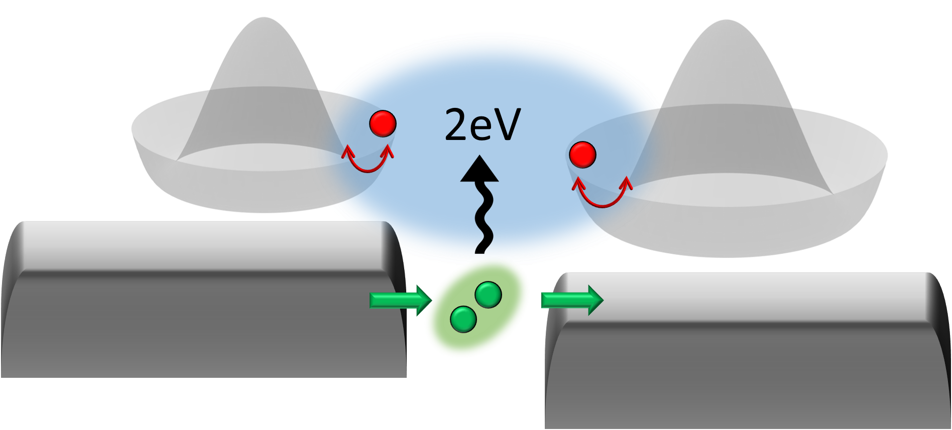
Figure 1: An illustration of the Higgs mode excited by the energy emitted by tunneling Cooper pairs (green balls) in a voltage-biased Josephson junction. The mexican hat potentials depict the free-energy of the order parameter (red balls). The minima/troughs correspond to the equilibrium gaps.

In this letter, we investigate the OP dynamics in highly transparent voltage-biased Josephson junctions, revealing signatures of the Higgs mode in the absence of any external irradiation. The Josephson effect [34, 35, 36, 37, 38, 39] is a quintessential example of coherent phase mode dynamics, which arises as the condensates of two superconductors are coupled by their interference in the barrier region, where the potential drops. For a constant voltage bias $V$, an oscillating supercurrent $\sim\sin(\omega_{J}t)$ is obtained, where $\omega_{J}=2eV$ is the Josephson frequency. We find that unlike an isolated superconductor, this Josephson coupling induces OP oscillations as it directly links the OP to the photons emitted by the tunneling Cooper pairs [40] via the Josephson phase difference [13, 41], obviating the need for external irradiation. Microscopically, these Higgs oscillations occur when Cooper pairs alternate between coherently breaking into constituent Bogoliubov quasiparticles over the superconducting energy gap and subsequently recombining, which requires energy $\geq 2\Delta_{0}$. Consequently, a resonance condition emerges, $\omega_{J}=\omega_{H}$, beyond which the voltage excites OP oscillations. This results in a Josephson current oscillating at $2\omega_{J}$, which supersedes its $2\omega_{J}$ counterpart from higher-order Josephson effects for large Josephson couplings. Furthermore, it may even dominate the usual $\omega_{J}$ component when the equilibrium gaps of the leads are sufficiently unequal. These findings offer a clear indication of Higgs oscillations in time-reversal symmetric Josephson junctions featuring single-band s-wave superconductors [42, 43, 44, 45, 46, 47, 48, 49, 50, 51, 52, 53, 54].

Phenomenology.– We elucidate the key concepts using a time-dependent Ginzburg Landau (TDGL) model [12, 13], with the free energy $F=F_{L}+F_{R}+F_{J}$, where,

$$\begin{split}F_{L/R}=&(\partial_{t}\Delta_{L/R})^{2}-\Big{(}a_{L/R}\Delta_{L/R}^{2}+\frac{b}{2}\Delta_{L/R}^{4}\Big{)},\\ F_{J}=&-J\Delta_{L}\Delta_{R}\cos(\omega_{J}t).\end{split}$$ (1)

Here $\Delta_{L/R}\in\Re$ are the uniform OPs in the left/right leads, $a_{L/R}=(T-T_{C,L/R})/T_{C,L/R}$ with $T_{C,L/R}$ being the critical temperature, and the Josephson coupling $J\sim\mathcal{T}^{2}$ where $\mathcal{T}$ parametrises the coupling across the junction. The equilibrium OPs, in the absence of the Josephson coupling, are obtained as $\Delta_{0,L/R}=\sqrt{-a_{L/R}/b}$. Microscopic calculations yield the Higgs mass $\omega_{H,L/R}=2\Delta_{0,L/R}$ [12, 13]. On expanding about the equilibrium OP values, $\Delta_{L/R}=\Delta_{0,L/R}+\delta\Delta_{L/R}$, we obtain,

$$\int_{-\infty}^{t}d\tau\begin{bmatrix}\chi_{L}^{-1}&s^{\prime}_{\phi,L}\\ s^{\prime}_{\phi,R}&\chi_{R}^{-1}\end{bmatrix}_{(t,\tau)}\begin{bmatrix}\delta\Delta_{L}\\ \delta\Delta_{R}\end{bmatrix}_{(\tau)}=\begin{bmatrix}s_{\phi,L}\\ s_{\phi,R}\end{bmatrix}_{(\tau)}$$ (2)

with $\chi^{-1}_{L/R}=(\partial_{t}^{2}+\omega_{H,L/R}^{2})\delta(t-\tau)$, $s^{\prime}_{\phi,L/R}=J\cos(\omega_{J}t)\delta(t-\tau)$, and $s_{\phi,L/R}=-J\Delta_{0,R/L}\cos(\omega_{J}t)\delta(t-\tau)$. This system of equations resembles driven coupled oscillators. The source term $s_{\phi}$ oscillates at the Josephson frequency $\omega_{J}$ for a constant voltage $V$. It captures the excitations provided by the radiating pairs traversing the junction. The cross terms $\sim s_{\phi}^{\prime}$ describe the coupling between the oscillating components of the two OPs, which are also driven by the junction field with $s^{\prime}_{\phi}$ oscillating at $\omega_{J}$. At leading order in $J$, when the cross-coupling may be neglected, we find $\delta\Delta_{L/R}^{(J)}(t)=\int_{-\infty}^{t}d\tau\chi_{L/R}(t,\tau)s_{\phi,L/R}(\tau)$. Since the susceptibility $\chi_{L/R}(\omega)=1/(-\omega^{2}+\omega_{H,L/R}^{2})$ is peaked at the Higgs frequency, $\delta\Delta_{L/R}$ oscillates at $\omega_{J}$, and exhibits a resonant enhancement for $\omega_{J}=\omega_{H,L/R}$, corresponding to the excitation of the Higgs mode. This is evident from the leading order solution $\delta\Delta_{L/R}^{(J)}=\frac{J\Delta_{0,R/L}}{\omega_{J}^{2}-\omega_{H,L/R}^{2}}\cos(\omega_{J}t)$. For larger values of $J$, the cross terms $\sim s_{\phi}^{\prime}$ become significant, generating a $\mathcal{O}(J^{2})$ correction, $\delta\Delta_{L/R}^{(J^{2})}=\iint_{-\infty}^{t}d\tau d\tau^{\prime}\chi_{L/R}(t,\tau)s_{\phi,L/R}^{\prime}(\tau,\tau^{\prime})\delta\Delta_{R/L}(\tau^{\prime})$. Due to the consequent interplay of the Higgs-enhanced OPs from each lead, the OPs within the two leads may oscillate at different frequencies in an asymmetric junction with $\Delta_{0,L}\neq\Delta_{0,R}$. Considering without loss of generality $\Delta_{0,L}<\Delta_{0,R}$, as the voltage is increased and $\omega_{J}$ approaches $\omega_{H,L}$, $\delta\Delta_{L}$ is Higgs-enhanced and becomes much larger than the non-resonant $\delta\Delta_{R}$ ($\omega_{H,R}>\omega_{H,L}$). The correction $\delta\Delta_{R}^{(J^{2})}\sim\chi_{R}s_{\phi,R}^{\prime}\delta\Delta_{L}$, which is otherwise suppressed by an extra factor of $J$ in $s_{\phi,R}^{\prime}$, becomes significant as the resonantly enhanced $\delta\Delta_{L}$ can compensate for the extra $J$. The combination of the $\omega_{J}$ oscillations in both $\delta\Delta_{L}$ and $s_{\phi^{\prime},R}$ results in a $2\omega_{J}$ component in $\delta\Delta_{R}$. However, $\delta\Delta_{L}^{(J^{2})}\sim\chi_{L}s_{\phi,L}^{\prime}\delta\Delta_{R}$ remains relatively suppressed due to the smallness of the off-resonant $\delta\Delta_{R}$. Thus, $\delta\Delta_{L}$ remains unchanged and still oscillates at $\omega_{J}$. This is readily observed in the solution to Eq. (2) presented in the Supplemental Material (SM) [55], which not only elaborates on the $\mathcal{O}(J^{2})$ perturbative solution, but also provides a numerical complement. Notably, in this asymmetric regime, the interplay of the Higgs enhancement and coupled Josephson dynamics strikingly manifest in a Josephson current with a much stronger $2\omega_{J}$ component, which may even dominate the the usual $\omega_{J}$ component. Within this TDGL analysis, the behaviour of the current may be readily obtained from the simple approximation $I\sim\Delta_{L}(t)\Delta_{R}(t)\sin(\omega_{J}t)$. Using the OPs described above, we find a $2\omega_{J}$ component in the current bearing the amplitude $I_{0}f_{H}$, where $I_{0}=\Delta_{0,L}\Delta_{0,R}$ is the amplitude of the usual $\omega_{J}$ component, and $f_{H}=-(J/2)(\Delta_{0,R}/\Delta_{0,L})/(-\omega_{J}^{2}+\omega_{H,L}^{2})$ is the Higgs enhancement factor [55]. This term arises from the product of the components dominating the OPs of each lead, namely, the constant $\Delta_{0,R}$ in the right lead, and the component oscillating at $\omega_{J}$ in the left lead. For the Higgs-resonance conditions mentioned earlier, this $2\omega_{J}$ component is sufficiently amplified to result in a predominant $2\omega_{J}$ Josephson current. Furthermore, even for equal equilibrium gaps $\Delta_{0,L}=\Delta_{0,R}=\Delta_{0}$, the same analysis shows that the $2\omega_{J}$ component in the current is Higgs-enhanced by the factor $J/(-\omega_{J}^{2}+\omega_{H}^{2})$, where $\omega_{H}=2\Delta_{0}$. However, in this case, even the usual $\omega_{J}$ component is enhanced by the factor $1+(J^{2}/4)/(-\omega_{J}^{2}+\omega_{H}^{2})^{2}$. This precludes a dominant $2\omega_{J}$ current. These calculations are detailed in the SM [55] for brevity.

Finally, we note that while it is intuitive to employ the TDGL formalism with the rather simple form of the Josephson energy [13], $F_{J}\sim\Delta_{L}(t)\Delta_{R}(t)\cos(\phi)$, where $\phi=\theta_{L}(t)-\theta_{R}(t)=2eVt$ is the Josephson phase-difference, it is nevertheless an approximation which holds for tunnel junctions with a small Josephson coupling, and $\phi$ varying much slower than the intrinsic microscopic dynamical variables [59]. In the present scenario, where the time-dependent OP oscillates at the same time scale as $\phi$, it is imperative to account for the proper retarded dynamics [58, 59, 60, 61]. This is the approach taken in the remainder of the article.

Model.– We consider the s-wave BCS superconducting Hamiltonian with attractive Gorkov point-contact interaction [62, 63], valid for energies much smaller than the Debye frequency. We analyse a single-channel Josephson junction, with two s-wave superconducting leads having $N_{1}$ sites each. Performing a mean-field decomposition, the action is written as, $S=S_{L}+S_{R}+S_{T}$, with

$$\begin{split}S_{L/R}=\int_{t}&\sum_{j\in L/R,\sigma}\frac{-\zeta}{2}\big{(}c_{j+1\sigma}^{\dagger}c_{j\sigma}+c_{j\sigma}^{\dagger}c_{j+1\sigma}\big{)}\\ +&\big{(}\Delta_{j}(t)c^{\dagger}_{j\sigma}c^{\dagger}_{j\sigma^{\prime}}+\Delta_{j}^{*}(t)c_{j\sigma^{\prime}}c_{j\sigma}\big{)}+\frac{\Delta_{j}(t)^{2}}{g},\end{split}$$ (3)

and

$$S_{T}=\int_{t}\sum_{\sigma}-\mathcal{T}\big{(}e^{i\phi(t)/2}c_{LN_{1}\sigma}^{\dagger}c_{R1\sigma}+e^{-i\phi(t)/2}c_{R1\sigma}^{\dagger}c_{LN_{1}\sigma}\big{)}.$$ (4)

Here, $\zeta$ is the hopping amplitude, $g>0$ quantifies the BCS attractive interaction, and $\phi(t)=(2e/\hbar)\int_{-\infty}^{t}d\tau V(\tau)$. We gauge out the applied bias potential, which is then shifted into the junction couplings [64]. Writing the action on the Keldysh contour, the saddle-point condition [65, 66] yields the non-equilibrium gap equation,

$$\Delta_{j}(t)=igF^{<}_{j,j}(t,t),$$ (5)

where $F^{<}$ is the anomalous component of the Nambu lesser Green’s function $G^{<}$.

We assume that prior to the gauge transformation, the phase of the OP is completely determined by the corresponding electro-chemical potentials. This leads to purely real values of $\Delta(t)$ following the gauge transformation. This assumption, which is tantamount to the validity of the second Josephson relation ($d\phi/dt=2eV/\hbar$), holds for bulk superconductors where electric fields are typically restricted to surfaces and normal/insulating components of the system [67, 68, 69, 70]. In this scheme, oscillations of the OP thus stem from amplitude oscillations, as opposed to those arising from an increasing phase.

The Keldysh Green’s functions are obtained numerically using [71, 72, 66],

$$\begin{split}G^{r}(t,t^{\prime})=&-i\Theta(t-t^{\prime})\mathbb{T}e^{-i\int_{t^{\prime}}^{t}d\tau H(\tau)}e^{-\frac{\Gamma}{2}|t-t^{\prime}|}\\ G^{<}(t,t^{\prime})=&\iint_{-\infty}^{t,t^{\prime}}d\tau d\tau^{\prime}G^{r}(t,\tau)\Sigma^{<}(\tau,\tau^{\prime})G^{a}(\tau^{\prime},t^{\prime}),\\ \Sigma^{<}(\tau,\tau^{\prime})=&\frac{-\Gamma}{2\pi}\frac{1}{\tau-\tau^{\prime}+i0^{+}},\end{split}$$ (6)

where $\mathbb{T}$ is the time-ordering operator, and $\Gamma$ accounts for the level-broadening, arising from, e.g., the relaxation to the high-energy quasiparticle continuum, external environments, electron-phonon interactions, or dissipation [61]. We numerically obtain a self-consistent solution for the OP $\Delta(t,x)$ from Eq. (5). We emphasise that this technique permits us to probe the full non-perturbative self-consistent dynamics, while making no assumptions regarding the smallness of any parameter, including $\mathcal{T}$. Finally, the current is obtained as [61, 64],

$$I=\sum_{\sigma}\frac{e(-\mathcal{T})}{\hbar}\Re\ \mathbf{Tr}e^{-i\frac{\phi(t)\tau_{Nz}}{2}}G_{R1,LN_{1},\sigma}^{<}(t,t),$$ (7)

where $\tau_{N\nu}$ is the $\nu^{\text{th}}$ Pauli matrix in Nambu space, and the subscripts $R1$ and $LN_{1}$ denote the first site of the right lead and the last site of the left lead, respectively.

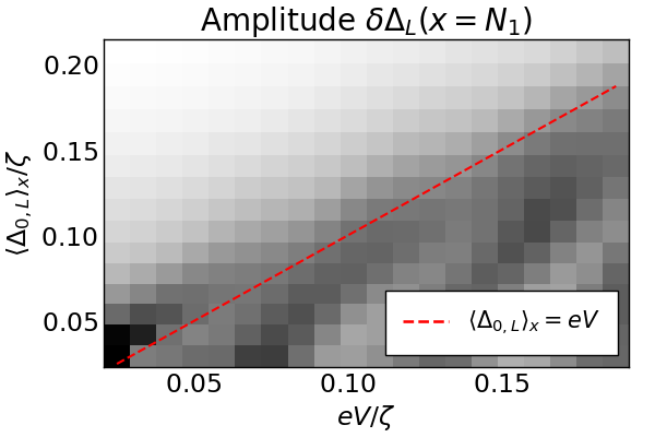
Figure 2: The amplitude of the OP oscillations, $\delta\Delta$ (arbitrary units), for a range of voltages, and mean OP in the left lead. We consider $N_{1}=26$ sites in each lead, $\mu=0$, $\Gamma=0.05\zeta$, $\mathcal{T}=0.075\zeta$, and $\Delta_{0,R}=0.248\zeta$ in the right lead (corresponding to $g=1.625\zeta$). The leading resonant behaviour is obtained when $2eV\approx 2\Delta_{0,L}$ (red dashed line), around which the amplitude rises (smoothened due to finite $\Gamma$).

Results.– We perform a perturbative analysis to motivate the dynamical behaviour of the OP. Starting with the equilibrium gap $\Delta_{0}$ ($V,\mathcal{T}=0$), we write $\Delta(t,x)=\Delta_{0}(x)+\delta\Delta(t,x)$. The corresponding self-energy is obtained as $\Sigma_{\delta\Delta}(t,x)=\delta\Delta(t,x)\tau_{Nx}$. The self energy related to the coupling $\mathcal{T}$ is given by $\Sigma_{T,LR}(t)=\Sigma_{T,RL}^{*}(t)=(-\mathcal{T})\tau_{Nz}\exp(-i\phi(t)\tau_{Nz}/2)$. Using the Dyson equation, we have up to $\mathcal{O}(\mathcal{T}^{2})$, $G_{L/R}^{<}=g_{L/R}^{<}+\sum_{j=1,2,3}\delta(G_{L/R}^{<})^{(j)}$. Here, $\delta(G_{L/R}^{<})^{(1)}$ has one instance of $\Sigma_{\delta\Delta}$, and accounts for the intrinsic dynamics of the pairs. It leads to the Higgs susceptibility. Instead, $\delta(G_{L/R}^{<})^{(2)}$ has two instances of $\Sigma_{T}$. It describes the effect of the radiating pairs tunneling across the junction. Finally, $\delta(G_{L/R}^{<})^{(3)}$ has one instance of $\Sigma_{\delta\Delta}$ and two instances of $\Sigma_{T}$. It captures the cross-coupling between the OP oscillations of the two leads mediated by the tunneling Cooper pairs. We specify them in the SM [55] for brevity. These considerations, along with Eq. (5), once again yield Eq. (2), albeit with modified forms of susceptibility, source, and cross terms, $\chi_{L}^{-1}(t-\tau)=\delta(t-\tau)-g\Im K_{1,L}(t-\tau)$, $K_{1,L}(t-\tau)=\frac{\partial\delta(G_{L}^{<})_{12}^{(1)}}{\partial\delta\Delta_{L}(\tau)}$, $s_{\phi,L}=(G_{L}^{<})^{(2)}$, and $s^{\prime}_{\phi,L}=\frac{\partial(G_{L}^{<})^{(3)}}{\partial\delta\Delta_{R}(\tau)}$.

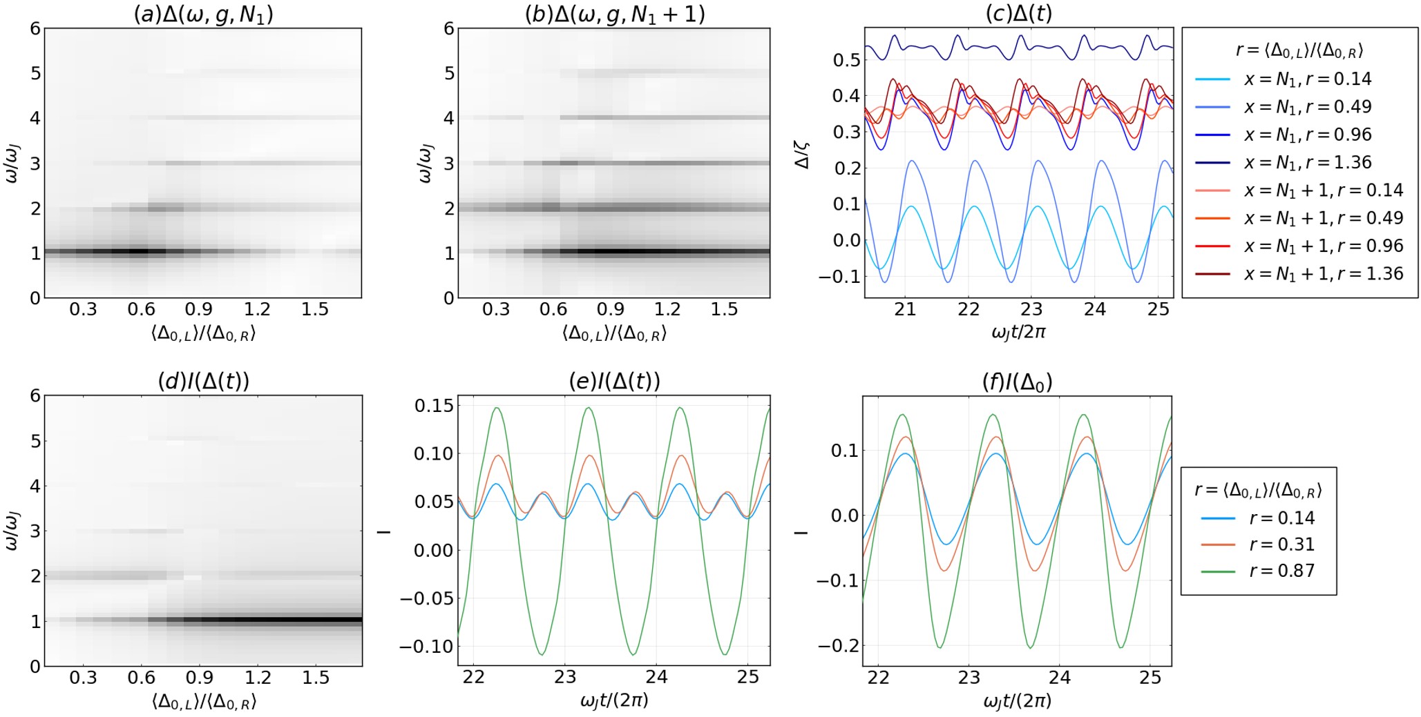
Figure 3: Numerically obtained results for varying $\langle\Delta_{0,L}\rangle$, while keeping $\langle\Delta_{0,R}\rangle$ constant. We consider $N_{1}=45$ sites in each lead, $\mu=0$, $\mathcal{T}=0.375\zeta$, $\Gamma=0.05\zeta$, and $eV=0.125\zeta$. (a-b) The spectral components of the OP (arbitrary units), at the sites immediately neighbouring the junction on the (a) left, and (b) right leads. (c) OP in time-domain. (d) Current (arbitrary units) calculated using the self-consistent OP (arbitrary units). For small values of $\langle\Delta_{0,L}\rangle/\langle\Delta_{0,R}\rangle$ we see a strong second-harmonic $2\omega_{J}=4eV$ response, which gives way to the usual dominant $\omega_{J}$ response as $\langle\Delta_{0,L}\rangle/\langle\Delta_{0,R}\rangle$ increases. (e,f) Current (arbitrary units) in time domain, using (e) self-consistent OP, and (f) equilibrium gaps (panels (e) and (f) share the same legend). In (e), for small $\langle\Delta_{0,L}\rangle/\langle\Delta_{0,R}\rangle$ we clearly see a dominant second harmonic response ($2\omega_{J}$).

Microscopically, $\chi$, and thus $K_{1}$, describe the inertia to changes in the OP, quantifying how the OP $\delta\Delta(t,x)$ is affected by disturbances in the past at other locations, $\delta\Delta(\tau\leq t,x^{\prime})$, due to the propagation of the corresponding changes in the quasiparticle distribution. While the exact form of $K_{1}$ is rather complicated, we see that it has oscillatory components with frequencies predominantly equal to and greater than $2\Delta_{0}$, corresponding to the spectral gap, while frequencies below $2\Delta_{0}$ are suppressed [55]. This spectral cut-off equalling $2\Delta_{0}$, albeit a smooth one due to finite $\Gamma$, represents the availability of quasiparticle states for the periodic breaking and forming of Cooper pairs above $2\Delta_{0}$, constituting the OP Higgs oscillations. We present the corresponding numerically obtained behaviour of $K_{1}$ in the SM [55]. Furthermore, $K_{1}$ has also contributions from the quasiparticle spectral weights extending all the way to the bandwidth [55], which result in decoherence due to the large range of frequencies corresponding to the time-evolution of the propagating quasiparticles. The crucial point is that, due to the spectral composition of $K_{1}$, the response $\delta\Delta(t)$ is largely dominated by frequencies greater than or equal to $2\Delta_{0}$. These fine details, arising from the microscopic retarded dynamics, are missed by the simple TDGL analysis introduced earlier. Both source and cross-coupling terms have two factors of $\exp(\pm i\phi/2)$, arising from the two instances of the junction coupling self-energy $\Sigma_{T}$. Thus they oscillate at the Josephson frequency $2eV$ [55]. Recall that the TDGL analysis yields the same feature. Thus, for small $\mathcal{T}$, we see that $\delta\Delta_{L/R}=\int^{t}d\tau\chi_{L/R}(t-\tau)s_{\phi}(\tau)$, which too oscillates at $2eV$. Additionally, noting that $\chi_{L/R}(t-\tau)\approx\delta(t-\tau)-g\Im K_{1,L}(t-\tau)$, we obtain a primary resonance condition when the oscillations of $s_{\phi}$ at the Josephson frequency matches the oscillations in $K_{1}$, i.e., $2eV=2\Delta_{0}$. As such, the $2eV$ energy emitted by a tunneling Cooper pair can excite the largest OP amplitude response.

The numerical solution of Eq. (5), which comprehensively captures the rich physics emerging from the inherent non-linearities of the problem, and is a necessity for accessing the non-perturbative regime with large $\mathcal{T}$, is presented in Fig. 3. As expected, in a junction with a large $\mathcal{T}$, the OP amplitude oscillations manifest as a disproportionately (relative to the case with constant OP, exhibiting higher-order Josephson effect) larger second harmonic component in the Josephson current oscillating at $2\omega_{J}$. Furthermore, the strength of the $2\omega_{J}$ component is commensurate with the value of $\mathcal{T}$, as well as asymmetry between $\Delta_{0,L}$ and $\Delta_{0,R}$, i.e., $|1-\Delta_{0,L}/\Delta_{0,R}|$. For sufficiently large values of these parameters, we obtain a transition when the $2\omega_{J}$ componennt starts dominating the $\omega_{J}$ component, as shown in the SM [55]. In this regime, as shown in Fig. 3, the OP in the lead with the smaller equilibrium gap oscillates at $\omega_{J}$ and its mean value collapses to zero, while the OP in the other lead oscillates at $2\omega_{J}$.

Discussion.– We have proposed a transport-based model exploiting dynamical Josephson physics for exciting and probing the amplitude mode in superconductors. This approach does not require any external irradiation. A prerequisite for this phenomenon is a large coupling between the two superconductors, equivalent to a normal-state transmission [64] close to one. In asymmetric junctions [73, 74, 75, 76, 77, 78] having sufficiently different equilibrium gaps, which may even be tuned experimentally [79, 78], the second Josephson harmonic oscillating at the twice the Josephson frequency dominates the current. As such, it may be readily observed, for instance, in the Josephson radiation [80, 81]. Remarkably, we find that these effects are robust to the presence of large broadening, for which we have used values as large as $\Gamma/\Delta_{0}\sim 0.2-0.3$ in our numerics, while typical experimentally relevant values are $\Gamma/\Delta_{0}\sim 10^{-3}-10^{-1}$ [82, 83]. Several experiments [84, 85, 86, 87] have already reported a disproportionately large second harmonic Josephson current, while pointing at the potential non-equilibrium dynamics.

Supplemental Material: Josephson Signatures of the Superconducting Higgs/Amplitude Mode

In this Supplemental Material, we present additional data and figures to supplement the claims in the main text. In Section S1, we provide details related to the time-dependent Ginzburg Landau analysis in the main text. In Section S2, we provide the perturbative expansion for the lesser Green’s function. We also present the numerically obtained behaviour of $K_{1}$ and $s_{\phi}$, which determine the driving term and the susceptibility of the OP oscillations, introduced in the perturbative analysis in the main text. In Section S3, we present additional data obtained using our numerically exact method. To highlight the conditions needed to clearly observe the Higgs signatures in the Josephson current, we show results for (A) varying junction coupling $\mathcal{T}$ for both unequal and equal equilibrium gaps, and (B) equilibrium gap ratio $\Delta_{0,L}/\Delta_{0,R}$ while keeping $\mathcal{T}$ fixed.

S1 TDGL analysis

Note that the equilibrium gap is given by $\Delta_{0,L/R}=\sqrt{-a_{L/R}/b}$. Since the Higgs mass is $2\Delta_{0,L/R}$, one must identify $-2a_{L/R}$ (Higgs mass obtained in the TDGL model) with $\omega_{H,L/R}^{2}=(2\Delta_{0,L/R})^{2}$ [1, 2].

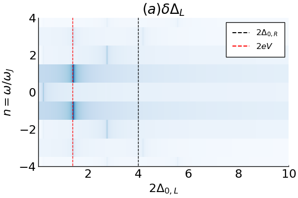
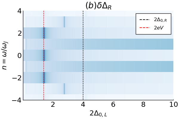
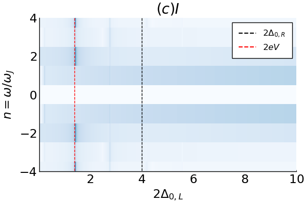
Figure S1: (color online) (a-b) $\delta\Delta_{L/R}(\omega=n\omega_{J})$ (we actually show $|\delta\Delta|^{0.25}$ for ease of viewing), as a function of the equilibrium gap $\Delta_{0,L}$ of the left lead, while $\Delta_{0,R}=2$ is kept fixed. We consider a bias $eV=0.7$, junction coupling $\mathcal{T}=0.75$, with the Josephson coupling $J=\mathcal{T}^{2}$. We observe two key features: (1) For small $\Delta_{0,L}$, $\delta\Delta_{L}(\omega)$ is peaked at $\pm 1\omega_{J}$, whereas $\delta\Delta_{R}(\omega)$ is peaked at $\pm 2\omega_{J}$. As $\Delta_{0,L}$ increases, both are peaked at $\pm\omega_{J}$. (2) The response is peaked at $2\Delta_{0,L}=2eV$, which is the expected (Higgs) resonant behaviour of the TDGL model. (c) The corresponding current (we actually show $|I|^{0.25}$ for ease of viewing), clearly showing a dominant $2\omega_{J}$ response for $\Delta_{0,L}\ll\Delta_{0,R}$ at the Higgs resonance condition $\omega_{J}=2eV=\omega_{H}=2\Delta_{0,L}$. For larger values of $\Delta_{0,L}$, we recover the usual $\omega_{J}$ current.

First, we present a perturbative solution to Eq. (2) in the main text. Since the equation contains drive terms with frequency $\omega_{J}$, the solution must have the same period. As such, we can expand $\delta\Delta_{L/R}(\omega)=\sum_{n}\delta\bar{\Delta}_{L/R,n}\delta(\omega-n\omega_{J})$, which transforms Eq. (2) to,

$$(-n^{2}\omega_{J}^{2}+\omega_{H,L}^{2})\delta\bar{\Delta}_{L,n}+\frac{J}{2}(\delta\bar{\Delta}_{R,n+1}+\delta\bar{\Delta}_{R,n-1})= -J\Delta_{0,R}(\delta_{n,1}+\delta_{n,-1}),$$ (S1)

$$(-n^{2}\omega_{J}^{2}+\omega_{H,R}^{2})\delta\bar{\Delta}_{R,n}+\frac{J}{2}(\delta\bar{\Delta}_{L,n+1}+\delta\bar{\Delta}_{L,n-1})= -J\Delta_{0,L}(\delta_{n,1}+\delta_{n,-1}).$$ (S2)

Following the corresponding discussion in the main text, we assume without loss of generality $\Delta_{0,L}\ll\Delta_{0,R}$. As $\omega_{J}$ approaches $\omega_{H,L}$, which implies $\delta\bar{\Delta}_{L,1}\gg\delta\bar{\Delta}_{R,1}$, at the leading order in $J$ we obtain,

$$\delta\bar{\Delta}_{L,\pm 1}= \frac{-J\Delta_{0,R}}{(-\omega_{J}^{2}+\omega_{H,L}^{2})},$$ (S3a)

$$\delta\bar{\Delta}_{R,\pm 1}= \frac{-J\Delta_{0,L}}{(-\omega_{J}^{2}+\omega_{H,R}^{2})},\quad(\delta\bar{\Delta}_{R,\pm 1}\ll\delta\bar{\Delta}_{L,\pm 1}\text{ for }\omega_{J}\to\omega_{H,L}),$$ (S3b)

$$\delta\bar{\Delta}_{R,\pm 2}= \frac{-\frac{J^{2}}{2}\Delta_{0,R}}{(-\omega_{J}^{2}+\omega_{H,L}^{2})(-4\omega_{J}^{2}+\omega_{H,R}^{2})},\quad(\delta\bar{\Delta}_{R,\pm 2}\gg\delta\bar{\Delta}_{R,\pm 1}\text{ for }\omega_{J}\to\omega_{H,L}).$$ (S3c)

The Higgs enhancement of $\delta\bar{\Delta}_{L,\pm 1}$ at $\omega_{J}=\omega_{H,L}$ compensates for the extra factor of $J$ and generates at $2\omega_{J}$ component in $\delta\Delta_{R}$, which can exceed its $\omega_{J}$ counterpart.

For equal equilibrium gaps, $\Delta_{0,L}=\Delta_{0,R}$, with equal Higgs frequency $\omega_{H}=2\Delta_{0}$, $\delta\Delta_{L}=\delta\Delta_{R}$. At the leading order in $J$, we obtain,

$$\delta\bar{\Delta}_{\pm 1}= \frac{-J\Delta_{0}}{(-\omega_{J}^{2}+\omega_{H}^{2})}.$$ (S4)

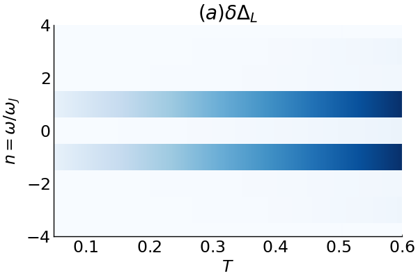
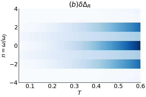
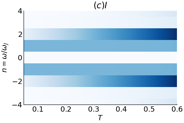
Figure S2: (color online) (a-b) $\delta\Delta_{L/R}(\omega=n\omega_{J})$ (we actually show $|\delta\Delta|^{0.5}$ for ease of viewing), as a function of the junction coupling $\mathcal{T}$, with $\Delta_{0,L}=0.5$, $\Delta_{0,R}=2$, $eV=0.4$, Josephson coupling $J=\mathcal{T}^{2}$. $\delta\Delta_{L}$ shows $\omega_{J}$ oscillations, whereas $\delta\Delta_{R}$ makes a transition to $2\omega_{J}$ oscillations with increasing $\mathcal{T}$(equivalently $J$). (c) Accordingly, with increasing $J$, the $2\omega_{J}$ component in the current (we actually show $|I|^{0.5}$ for ease of viewing) starts dominating.

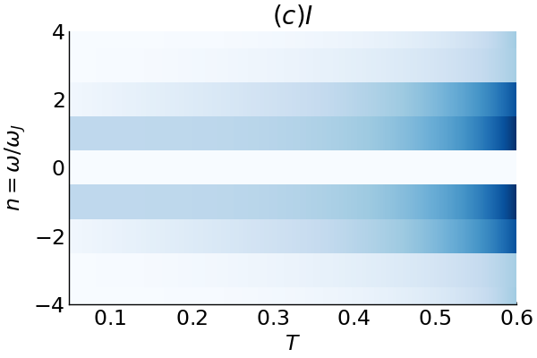
Figure S3: (color online) (a-b) Same as Fig. S2, but this time with $\Delta_{0,L}=\Delta_{0,R}=0.5$. Both $\delta\Delta_{L}$ and $\delta\Delta_{R}$ are dominated by $\omega_{J}$ oscillations throughout. (c) Even though the $2\omega_{J}$ component in the current strengthens significantly, it is nevertheless dominated by the $\omega_{J}$ component.

Now, (S3) may be applied to obtain the behaviour of the current using the simple expression $I\sim\Delta_{L}(t)\Delta_{R}(t)\sin(\omega_{J}t)$.

$$I= \big{(}\Delta_{L,0}+\delta\bar{\Delta}_{L,1}\cos(\omega_{J}t)\big{)}\big{(}\Delta_{R,0}+\delta\bar{\Delta}_{R,2}\cos(2\omega_{J}t)\big{)}\sin(\omega_{J}t)$$

$$\approx \Big{(}\Delta_{L,0}\Delta_{R,0}-\frac{1}{2}\Delta_{L,0}\delta\bar{\Delta}_{R,2}\Big{)}\sin(\omega_{J}t)+\frac{1}{2}\Delta_{R,0}\delta\bar{\Delta}_{L,1}\sin(2\omega_{J}t)+\frac{1}{2}\Delta_{L,0}\delta\bar{\Delta}_{R,2}\sin(3\omega_{J}t)+\ldots$$

$$\approx \Delta_{L,0}\Delta_{R,0}\sin(\omega_{J}t)+\frac{1}{2}\Delta_{R,0}\delta\bar{\Delta}_{L,1}\sin(2\omega_{J}t).$$ (S5)

The $2\omega_{J}$ component in the current is propotional to $\Delta_{0,R}\delta\bar{\Delta}_{L,1}=-\Delta_{0,R}^{2}\frac{J}{(-\omega_{J}^{2}+\omega_{H,L}^{2})}$. For a sufficiently large $J$, and $\omega_{J}$ close to $\omega_{H,L}$ (corresponding to the Higgs resonance of the left lead), this $2\omega_{J}$ component can be resonantly enhanced and large enough to result in a predominant $2\omega_{J}$ Josephson current.

Furthermore, even for equal equilibrium gaps $\Delta_{0,L}=\Delta_{0,R}=\Delta_{0}$, the same analysis shows that the $2\omega_{J}$ component in the current has the amplitude $\sim\Delta_{0}\delta\bar{\Delta}_{1}=-\Delta_{0}^{2}J/(-\omega_{J}^{2}+\omega_{H}^{2})$. However, in this case both the leads have equally large oscillatory Higgs-resonant components $\delta\bar{\Delta}_{1}$, as they have equal gaps and hence the same Higgs frequency. This ends up enhancing the usual $\omega_{J}$ component of the current too, which arises from the product of the oscillatory components of the two leads. As a result, an outright domination of the $2\omega_{J}$ component is precluded.

$$I= \big{(}\Delta_{0}+\delta\bar{\Delta}_{1}\cos(\omega_{J}t)\big{)}^{2}\sin(\omega_{J}t)$$

$$\approx \Big{(}\Delta_{0}^{2}+\frac{1}{4}\delta\bar{\Delta}_{1}^{2}\Big{)}\sin(\omega_{J}t)+\Delta_{0}\delta\bar{\Delta}_{1}\sin(2\omega_{J}t)+\frac{1}{4}\delta\bar{\Delta}_{1}^{2}\sin(3\omega_{J}t).$$ (S6)

These results/trends are confirmed by the numerical solution to Eq. (2) in the frequency domain, as presented in Figs. S1, S2, and S3.

S2 Perturbative analysis

S2.1 Dyson expansion of $G^{<}$

$$\begin{split}&(G_{L}^{<})^{(1)}=\big{(}g_{L}^{r}\cdot\Sigma_{\delta\Delta_{L}}\cdot g_{L}^{<}+g_{L}^{<}\cdot\Sigma_{\delta\Delta_{L}}\cdot g_{L}^{a}\big{)},\\ &(G_{L}^{<})^{(2)}=\sum_{\begin{subarray}{c}l_{1..3}=\{<aa,\\ \ r<a,\ rr<\}\end{subarray}}g_{L}^{l_{1}}\cdot\Sigma_{T,LR}\cdot g_{R}^{l_{2}}\cdot\Sigma_{T,RL}\cdot g_{L}^{l_{3}},\\ &(G_{L}^{<})^{(3)}=\sum_{\begin{subarray}{c}m_{1..4}=\\ \{<aaa,\ r<aa,\\ rr<a,\ rrr<\}\end{subarray}}\begin{split}\huge g_{L}^{m_{1}}\cdot\Sigma_{T,LR}\cdot g_{R}^{m_{2}}\cdot\Sigma_{\delta\Delta_{R}}\cdot g_{R}^{m_{3}}\\ \cdot\Sigma_{T,RL}\cdot g_{L}^{m_{3}}\end{split},\end{split}$$ (S7)

where the lowercase letter denote the bare Green’s functions, and the products are convolutions in space and time.

S2.2 $K_{1}$

In this section we present numerically obtained values for the quantity $K_{1}$ defined in the main text. In order to obtain $K_{1}$, we find $\delta G^{<}_{\delta\Delta,12}(t,t;x,x)=(g_{L}^{r}*\Sigma_{\Delta}*g_{L}^{<}+g_{L}^{<}*\Sigma_{\Delta}*g_{L}^{a})|_{12}=\int_{-\infty}^{t}d\tau\int dx^{\prime}K_{1}(t-\tau;x,x^{\prime})\delta\Delta(x^{\prime},\tau)$ with $\mathcal{T}=0$, and obtain $K_{1}(t-\tau;x,x^{\prime})=\partial\delta G^{<}_{\delta\Delta,12}(t,t;x,x)/\partial\delta\Delta(\tau,x^{\prime})$. The subscript $12$ denotes the components of the $2\times 2$ matrix in the Nambu space. We find $\delta G^{<}_{\delta\Delta}(t,t;x,x)$ from $G^{<}$ calculated using Eq. (6), with $\mathcal{T}=0$ and $\Delta(x,t)=\Delta_{0}(x)+\delta\Delta(x,t)$, where $\delta\Delta(x,t)\ll\Delta_{0}$.

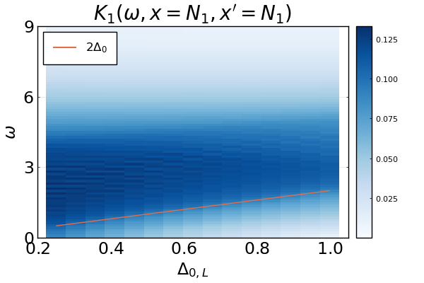
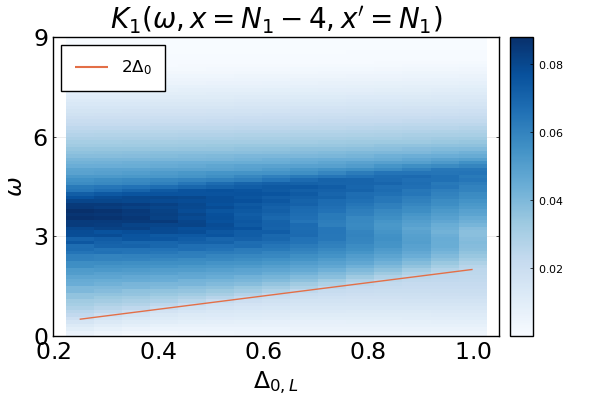
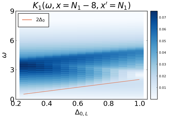
Figure S4: (color online) $K_{1}(t-\tau;x,x^{\prime})$, presented in Fourier domain as $K_{1}(\omega;x,x^{\prime})$ to show the spectral composition. We consider $N_{1}=60$ sites in each lead, $\zeta=4$, $\mu=0$, $\Gamma=0.1$, and a uniform equilibrium gap $\Delta_{0,R}=0.5$, while we vary $\Delta_{0,L}$ (uniform in each lead, not self-consistently determined). We show the result for $\delta\Delta_{0}=0.1$, located at the edge of a lead at the site indexed as $N_{1}$. The spectral gap in the Hamiltonian suppresses frequencies smaller than $2\Delta_{0}$ in $K_{1}(\omega;x,x^{\prime})$. There are, still, non-zero weights for frequencies below $2\Delta_{0}$ due to the contributions coming from the quasiparticle bands extending all the way to the bandwidth (see Eq. (S10) and the associated text).

Using $g^{r}(t)=\Theta(t)(g^{>}(t)-g^{<}(t))$ and $g^{a}(-t)=-\Theta(t)(g^{>}(t)-g^{<}(t))$, we see that

$$K_{1}(t-\tau;x,x^{\prime})= \Theta(t-\tau)\big{[}g_{11}^{>}(t-\tau;x-x^{\prime})g_{22}^{<}(\tau-t;x^{\prime}-x)-g_{11}^{<}(t-\tau;x-x^{\prime})g_{22}^{>}(\tau-t;x^{\prime}-x)$$

$$\hskip 28.45274pt+g_{12}^{>}(t-\tau;x-x^{\prime})g_{12}^{<}(\tau-t;x^{\prime}-x)-g_{12}^{<}(t-\tau;x-x^{\prime})g_{12}^{>}(\tau-t;x^{\prime}-x)\big{]},$$ (S8)

$$= \Theta(t-\tau)\int\frac{d\omega}{2\pi}e^{-i\omega(t-\tau)}\Bigg{[}\int\frac{d\Omega}{2\pi}\bigg{\{}A_{x,x^{\prime}}\bigg{(}\Omega+\frac{\omega}{2}\bigg{)}A_{x,x^{\prime}}\bigg{(}\Omega-\frac{\omega}{2}\bigg{)}+B_{x,x^{\prime}}\bigg{(}\Omega+\frac{\omega}{2}\bigg{)}B_{x,x^{\prime}}\bigg{(}\Omega-\frac{\omega}{2}\bigg{)}\bigg{\}}$$

$$\hskip 126.04572pt\times\bigg{\{}f\bigg{(}\Omega+\frac{\omega}{2}\bigg{)}-f\bigg{(}\Omega-\frac{\omega}{2}\bigg{)}\bigg{\}}\Bigg{]}$$ (S9)

where $g^{r}_{11}(\omega;x-x^{\prime})-g^{a}_{11}(\omega;x-x^{\prime})=iA_{x,x^{\prime}}(\omega)$ and $g^{r}_{12}(\omega;x-x^{\prime})-g^{a}_{12}(\omega;x-x^{\prime})=iB_{x,x^{\prime}}(\omega)$. The subcripts $11,12\ldots$ denote the components of the $2\times 2$ matrix in Nambu space. In the second line we have used the spectral decomposition: $g_{ab}^{<}(\omega)=(g_{ab}^{r}(\omega)-g_{ab}^{a}(\omega))(-f(\omega))$ and $g_{ab}^{>}(\omega)=(g_{ab}^{r}(\omega)-g_{ab}^{a}(\omega))(1-f(\omega))$. The factor $g_{ab}^{r}(\omega)-g_{ab}^{a}(\omega)=iA_{ab}(\omega)$ defines the spectral function. For $a=b$, i.e., equal spatial indices, it is the usual spectral density of states. In any case, for s-wave superconductors $A_{ab}(\omega)$ has a gap for $|\omega|<\Delta_{0}$, along with a singular edge at $|\omega|=\Delta_{0}$. The spectral gap in the spectral functions in this expression results in a spectral gap below $2\Delta_{0}$ in $K_{1}(\omega;x,x^{\prime})$. The gap-edges are smoothened for a finite $\Gamma$ For a wide-band BCS s-wave superconductor, it is possible to obtain a closed-form expression for $K_{1}$ when $x^{\prime}=x$. On using the results in Refs. [3, 4],

$$K_{1}(t-\tau;x,x^{\prime}=x)= i\Theta(t-\tau)\bigg{[}\frac{\hbar}{eR_{N}}\frac{d\delta(t-\tau)}{dt}-\frac{\pi\Delta_{0}^{2}}{2e\hbar R_{N}}\bigg{(}J_{1}\Big{(}\frac{\Delta_{0}t}{\hbar}\Big{)}Y_{1}\Big{(}\frac{\Delta_{0}t}{\hbar}\Big{)}+Y_{1}\Big{(}\frac{\Delta_{0}t}{\hbar}\Big{)}J_{1}\Big{(}\frac{\Delta_{0}t}{\hbar}\Big{)}\bigg{)}$$

$$\hskip 43.53271pt-\frac{\pi\Delta_{0}^{2}}{2e\hbar R_{N}}\bigg{(}J_{0}\Big{(}\frac{\Delta_{0}t}{\hbar}\Big{)}Y_{0}\Big{(}\frac{\Delta_{0}t}{\hbar}\Big{)}+Y_{0}\Big{(}\frac{\Delta_{0}t}{\hbar}\Big{)}J_{0}\Big{(}\frac{\Delta_{0}t}{\hbar}\Big{)}\bigg{)}\bigg{]},$$ (S10)

where $R_{N}$ is the normal state resistance. It oscillates at frequencies $2\Delta_{0}$. Note that since $K_{1}$ arises from the leading term in the perturbation expansion with $\delta\Delta\neq 0$ but $\mathcal{T}=0$, for $x$ in a given lead, $K_{1}$ is non-zero only for $x^{\prime}$ belonging to the same lead. Also, its oscillation frequency is determined by the equilibrium gap $\Delta_{0}$ of the same lead. The overlap of the quasiparticle bandtails in $A$, extending all the way to the bandwidth, creates a broad spectrum of frequencies in $K_{1}(\omega;x,x^{\prime})$, extending approximately to a height $\zeta$ over $2\Delta_{0}$, as seen in Fig. S4.

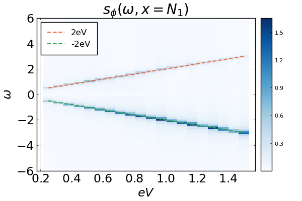
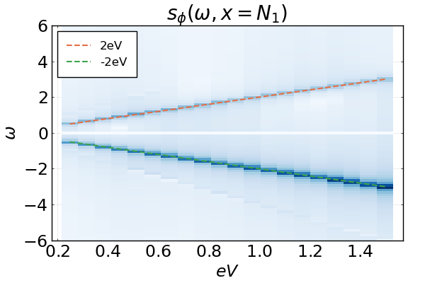
(a) (b)

Figure S5: (color online) $s_{\phi}(t,X=N_{1})$, presented in Fourier domain. We have considered $N_{1}=30$ sites in each lead, $\zeta=4$, $\mu=0$, $\Gamma=0.125$, and (a) a uniform $\Delta_{0}=0.5$ (equal in both leads), and (b), $\Delta_{0,L}=0.5$, $\Delta_{0,R}=0.5$ (uniform in each lead). In both cases, the gaps are not self-consistently determined. The dashed lines denote the Josephson frequency $2eV$.

S2.3 $s_{\phi}$

In this section we present numerically obtained values for the quantity $s_{\phi}$ defined in the main text, using Eq. (S7). In order to obtain $s_{\phi}$, we find $\delta G^{<}_{\mathcal{T}}(t,t;x,x)$ with $\delta\Delta=0$, with a small value of $\mathcal{T}$, and finally take the $12$ component in the Nambu space, i.e., $\delta G^{<}_{\mathcal{T},12}(t,t;x,x)$.

S3 Numerical analysis

S3.1 Varying junction coupling $\mathcal{T}$

S3.1.1 Unequal equilibrium gaps

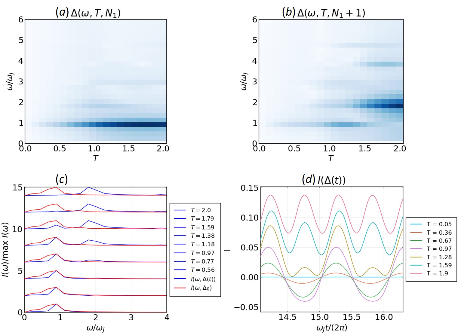
Figure S6: (color online) Numerically obtained results for varying $\mathcal{T}$. We consider $N_{1}=45$ sites in each lead, $\zeta=4$, $\mu=0$, $\Gamma=0.2$, and BCS attarctive couplings $g=5$ and $g=9$ in the left and right leads, repectively. (a-b) Spectral components of the OP (arbitrary units), at the sites immediately neighbouring the junction in the (a) left, and (b) right leads. (c) The normalised Fourier spectrum $I(\omega)/\text{max}I(\omega)$ for the current using (not using) self-consistently determined time-dependent OP in blue(red). The curves are shifted upwards by an amount proportional to the corresponding $\mathcal{T}$ for ease of viewing. With increasing $\mathcal{T}$, the $2\omega_{J}$ component dominates the spectrum. (d) The current in time domain (arbitrary units), for a range of $\mathcal{T}$.

S3.1.2 Equal equilibrium gaps

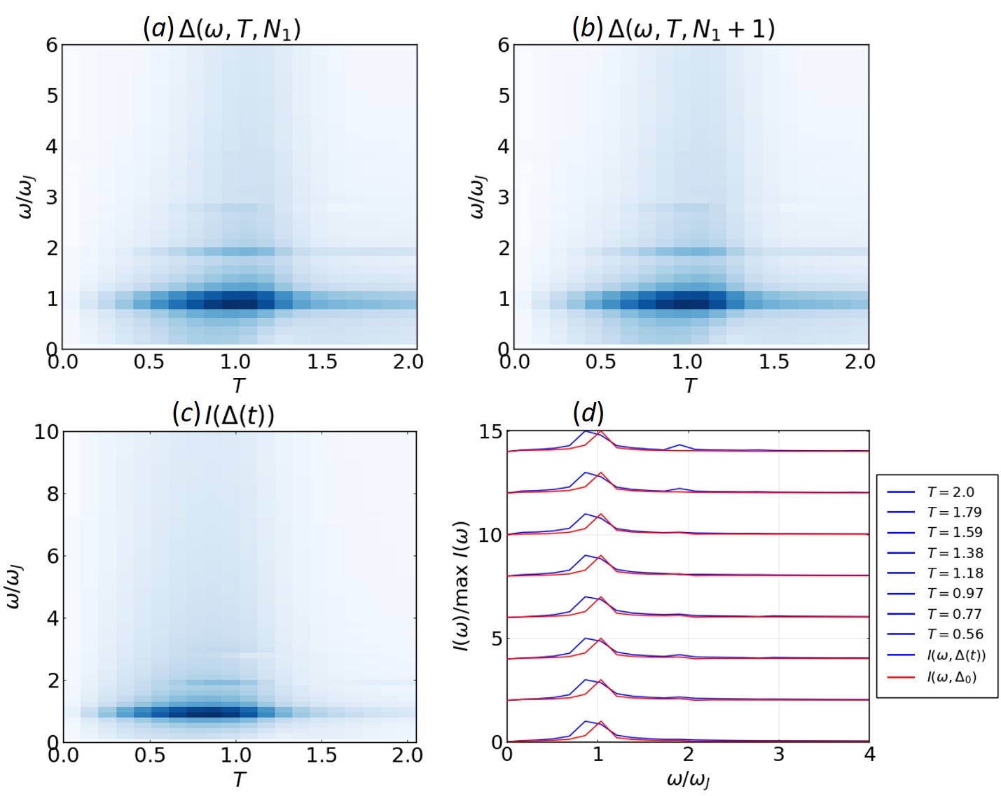
Figure S7: (color online) Numerically obtained results for varying $\mathcal{T}$. We consider $N_{1}=45$ sites in each lead, $\zeta=4$, $\mu=0$, $\Gamma=0.2$, and BCS attarctive couplings $g=5$ in both leads. (a-b) Spectral components of the OP (arbitrary units), at the sites immediately neighbouring the junction in the (a) left, and (b) right leads. (c) Current (arbitrary units) using the self-consistent OP (arbitrary units). The standard $\omega_{J}=2eV$ response dominates throughout, however, the $2\omega_{J}$ response becomes stronger than what is expected for the time independent OP with increasing $\mathcal{T}$ (higher order Josephson effect). This is seen clearly in (d), where we show the normalised Fourier spectrum of the current for specific values of $\mathcal{T}$. The curves are shifted up for ease of viewing, with the shifts being proportional to the corresponding $\mathcal{T}$.

S3.2 Varying equilibrium gap ratio $\Delta_{0,L}/\Delta_{0,R}$

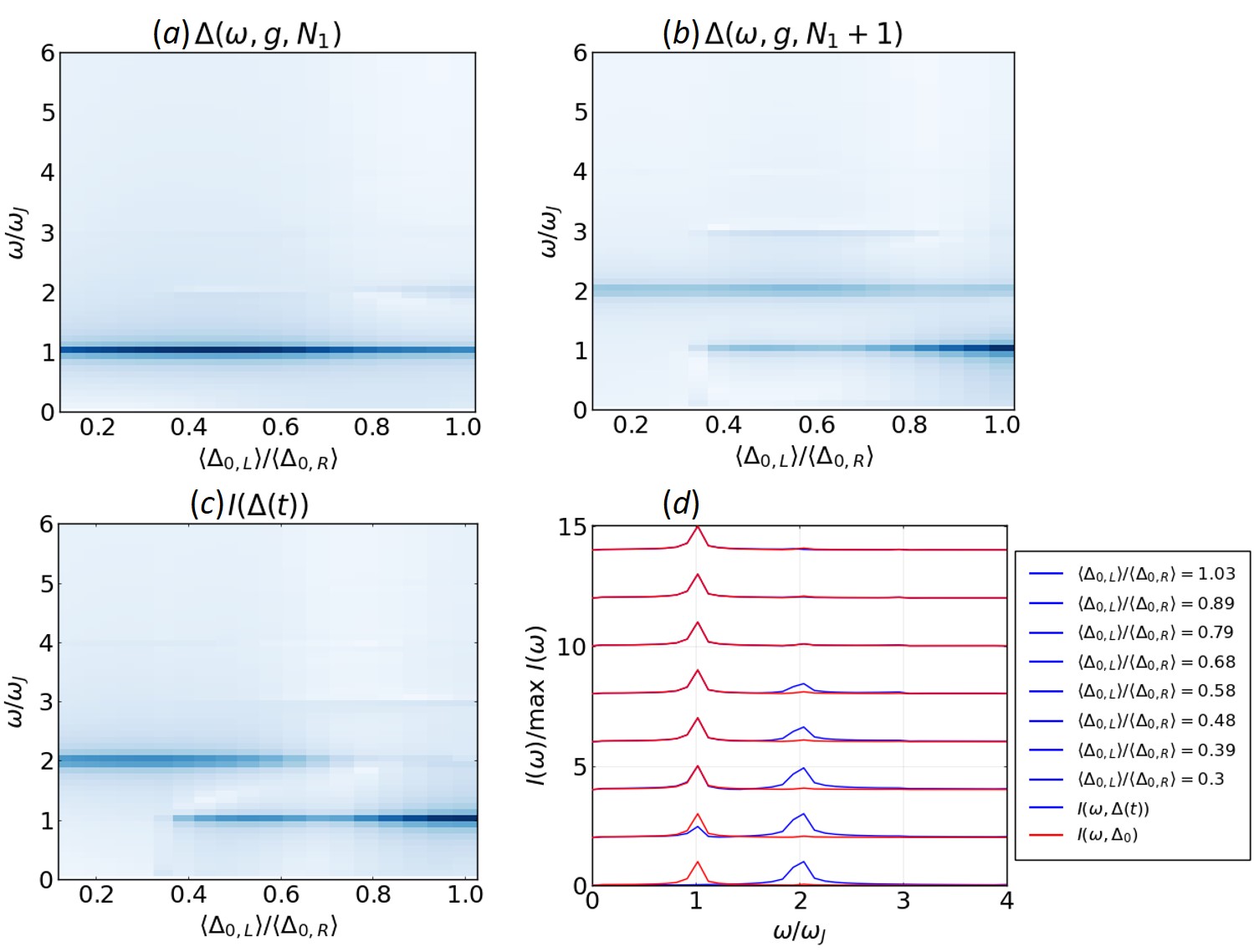
Figure S8: (color online) Numerically obtained results for varying $\Delta_{0,L}$. We consider $N_{1}=30$ sites in each lead, $\zeta=4$, $\mu=0$, $\mathcal{T}=1.5$, $\Gamma=0.2$, and BCS attractive coupling $g=6$ in the right lead. (a-b) Spectral components of the OP (arbitrary units), at the sites immediately neighbouring the junction in the (a) left, and (b) right leads. (c) Current (arbitrary units) using the self-consistent OP (arbitrary units). For small values of $\Delta_{0,L}/\Delta_{0,R}$ we see a dominant $2\omega_{J}$ response, which transitions into the usual $\omega_{J}$ response with increasing $\Delta_{0,L}/\Delta_{0,R}$. (d) The normalised Fourier spectrum $I(\omega)/\text{max}I(\omega)$ for the current using (not using) self-consistently determined time-dependent OP in blue(red). We consider various values of $\Delta_{0,L}/\Delta_{0,R}$. The curves are shifted up for ease of viewing, with the shifts being proportional to the corresponding $\Delta_{0,L}/\Delta_{0,R}$. For small values of $\Delta_{0,L}/\Delta_{0,R}$, corresponding to the lower curves, we note the much stronger $2\omega_{J}$ response.

References

[1] J.-J. Chang, and D.Scalapino, Nonequilibrium superconductivity. J. Low Temp. Phys. 31, 1–32 (1978).
[2] N. Kopnin, Theory of Nonequilibrium Superconductivity (Oxford University Press, New York, 2001).
[3] M. Tinkham, Non-Equilibrium Superconductivity in Festkörperprobleme (Advances in Solid State Physics, Vol. XIX), J. Treusch, ed. (Vieweg Braunschweig, 1979), p. 363.
[4] D. Fausti, R. I. Tobey, N. Dean, S. Kaiser, A. Dienst, M. C.
Hoffmann, S. Pyon, T. Takayama, H. Takagi, and A. Cavalleri, Science 331, 189 (2011).
[5] M. Mitrano, A. Cantaluppi, D. Nicoletti, S. Kaiser, A. Perucchi,
S. Lupi, P. Di Pietro, D. Pontiroli, M. Ricc‘o, S. R. Clark, D. Jaksch, and A. Cavalleri, Nature 530, 461 (2016).
[6] F. Giorgianni, T. Cea, C. Vicario, C. P. Hauri, W. K. Withanage, X. Xi, and L. Benfatto, Nat. Phys. 15, 341–346 (2019).
[7] R. Matsunaga and R. Shimano, Phys. Rev. Lett. 109, 187002 (2012).
[8] R. Matsunaga, Y. I. Hamada, K. Makise, Y. Uzawa, H. Terai, Z. Wang, and R. Shimano, Phys. Rev. Lett. 111, 057002 (2013).
[9] M. Beck, I. Rousseau, M. Klammer, P. Leiderer, M. Mittendorff, S. Winnerl, M. Helm, G. N. Gol’tsman, and J. Demsar, Phys. Rev. Lett. 110, 267003 (2013)
[10] R. Matsunaga, N. Tsuji, H. Fujita, A. Sugioka, K. Makise, Y. Uzawa, H. Terai, Z. Wang, H. Aoki, and R. Shimano, Science 345, 1145 (2014).
[11] P. W. Higgs, Phys. Rev. Lett. 13, 508 (1964).
[12] C. Varma, J. Low. Temp. Phys. 126, 901 (2002).
[13] D. Pekker and C. Varma, Annu. Rev. Condens. Matter Phys 6, 269 (2015).
[14] R. Shimano and N. Tsuji, Ann. Rev. Condens. Matter Phys. 11, 103 (2020).
[15] R. Matsunaga, N. Tsuji, K. Makise, H. Terai, H. Aoki, and R. Shimano, Phys. Rev. B 96, 020505 (2017).
[16] K. Katsumi, N. Tsuji, Y. I. Hamada, R. Matsunaga, J. Schneeloch, R. D. Zhong, G. D. Gu, H. Aoki, Y. Gallais, and R. Shimano, Phys. Rev. Lett. 120, 117001 (2018).
[17] P. W. Anderson, Phys. Rev. 110, 827 (1958).
[18] L. Schwarz, PhD thesis, Freie Universität Berlin (2020).
[19] D. Sherman, U. S. Pracht, B. Gorshunov, S. Poran, J. Jesudasan, M. Chand, P. Raychaudhuri, M. Swanson, N. Trivedi, A. Auerbach, et al., Nat. Phys. 11, 188 (2015).
[20] H. Chu, M.-J. Kim, K. Katsumi, S. Kovalev, R. D. Dawson, L. Schwarz, N. Yoshikawa, G. Kim, D. Putzky, Z. Z.
Li, et al., Nat. Commun. 11, 1793 (2020).
[21] C. Vaswani, J. Kang, M. Mootz, L. Luo, X. Yang, C. Sundahl, D. Cheng, C. Huang, R. H. Kim, Z. Liu, et al., Nat. Commun. 12, 258 (2021).
[22] R. Sooryakumar, and M. Klein, Phys. Rev. Lett. 45, 660 (1980).
[23] M.-A. Méasson, Y. Gallais, M. Cazayous, B. Clair, P. Rodiére, L. Cario, and A. Sacuto, Phys. Rev. B 89, 060503 (2014).
[24] T. Cea and L. Benfatto, Phys. Rev. B 90, 224515 (2014).
[25] R. Grasset, T. Cea, Y. Gallais, M. Cazayous, A. Sacuto, L. Cario, L. Benfatto, and M.-A. Méasson, Phys. Rev. B 97, 094502 (2018).
[26] M. A. Silaev, R. Ojajärvi, and T. T. Heikkilä, Phys. Rev. Res. 2, 033416 (2020).
[27] G. Tang, W. Belzig, U. Zülicke, and C. Bruder, Phys. Rev. Research 2, 022068 (2020).
[28] P. Vallet and J. Cayssol, Phys. Rev. B 108, 094515 (2023).
[29] V. Plastovets, A. S. Mel’nikov, and A. I. Buzdin, Phys. Rev. B 108 104507 (2023).
[30] M. Heckschen and B. Sothmann, Phys. Rev. B 105 045420 (2022).
[31] P. Derendorf, A. F. Volkov, and I. M. Eremin, Phys. Rev. B 109, 024510 (2024)
[32] Y. Li, M. Dzero, arXiv preprint arXiv:2311.09310 (2023).
[33] T. Kuhn, B. Sothmann, J. Cayao, arXiv preprint arXiv:2312.13785 (2023).
[34] B. D. Josephson, Phys. Lett. 1,
7, 251–253 (1962).
[35] B. D. Josephson, Rev. Mod. Phys. 36,
1, 216–220 (1964).
[36] B. D. Josephson, Adv. Phys. 14,
56, 419–451 (1965).
[37] P. W. Anderson and J.M. Rowell, Phys. Rev. Lett. 10,
6, 230–232 (1963).
[38] J. M. Rowell, Phys. Rev. Lett. 11,
5, 200–202 (1963).
[39] I. K. Yanson, V. M. Svistunov and I. M. Dmitrenko, Zh.
E´ksp. Teor. Fiz. 48, 976 (1965) [Sov. Phys. JETP 21, 650 (1965)].
[40] M. Hofheinz, F. Portier, Q. Baudouin, P. Joyez, D. Vion, P. Bertet, P. Roche, and D. Esteve Phys. Rev. Lett. 106, 217005 (2011).
[41] T. Klapwijk, G. Blonder and M. Tinkham, Physica B + C 109, 1657–1664 (1982).
[42] In time-reversal symmetric single-band s-wave superconductors, there remains no other mechanism for enhancing the component, or suppressing the component. However, as detailed in Refs. [43, 44, 45, 46, 47, 48, 49, 50, 51, 52, 53, 54].
this may be possible in cases with ferromagnetic components, spin-orbit interaction in the presence of a magnetic field, d- and p- wave superconductors, and multiband superconductors
[43] H. Sellier, C. Baraduc, F. Lefloch and R. Calemczuk, Phys. Rev. Lett. 92, 257005 (2004).
[44] H. Sickinger, A. Lipman, M. Weides, R. G. Mints, H. Kohlstedt, D. Koelle, R. Kleiner and E. Goldobin, Phys. Rev. Lett. 109, 107002 (2012).
[45] E. Goldobin, D. Koelle, R. Kleiner and A. Buzdin, Phys. Rev. B 76, 224523 (2007).
[46] S. M. Frolov, D. J. Van Harlingen, V. V. Bolginov, V. A. Oboznov, and V. V. Ryazanov, Phys. Rev. B 74, 020503(R) (2006).
[47] F. Li, L. Wu, L. Chen, S. Zhang, W. Peng, and Z. Wang, Phys. Rev. B 99, 100506(R) (2019).
[48] T. Yokoyama, M. Eto, and Y. V. Nazarov, Phys. Rev. B 89, 195407 (2014).
[49] Y. Tanaka and S. Kashiwaya, Phys. Rev. B 56, 892 (1997).
[50] T. K. Ng, and N. Nagaosa, EPL 87, 17003 (2009).
[51] Y. Asano, Y. Tanaka, M. Sigrist, and S. Kashiwaya, Physical Review B 67, 184505 (2003).
[52] C. J. Trimble, M. T. Wei, N. F. Q. Yuan, S. S. Kalantre, P. Liu, H.-J. Han, M.-G. Han, Y. Zhu, J. J. Cha, L. Fu, and J. R. Williams, npj Quantum Materials 6, 61 (2021).
[53] O. Can, T. Tummuru, R. P. Day, I. Elfimov, A. Damascelli, and M. Franz, Nature Physics 17, 519 (2021).
[54] T. Tummuru, S. Plugge, and M. Franz, Phys. Rev. B 105, 064501 (2022).
[55] See Supplemental Material, which includes Refs. [46-47], for additional details regarding the TDGL and perturbative analysis in the main text, and numerical results showing the behaviour of the OPs and the current with varying junction coupling and asymmetry between the equilibrium gaps.
[56] R. E. Harris, Phys. Rev. B. 13, 9, 3818-3829 (1975).
[57] D. V. Averin, Phys. Rev. Research. 3, 4, 043218 (2021).
[58] A. I. Larkin and Y. N. Ovchinnikov, Zh. Eksp. Teor. Fiz. 51, 1535 [Sov. Phys. JETP 24, 1035 (1967)].
[59] V Ambegaokar, U Eckern, and G Schön, Phys. Rev. Lett. 48, 1745 (1982).
[60] N. R. Werthamer, Phys. Rev. 147, 255 (1966).
[61] A. Lahiri, S.-J. Choi, and B. Trauzettel, Phys. Rev. Lett. 131, 126301 (2023).
[62] A. A. Abrikosov, L. P. Gorkov, and I. E. Dzyaloshinski, Methods of Quantum Field Theory in Statistical Physics (Dover, New York, 1975).
[63] G. Stefanucci, E. Perfetto and M. Cini, J. Phys.: Conf. Ser. 220 012012 (2010).
[64] J. C. Cuevas, A. Martín-Rodero, and A. Levy Yeyati, Phys. Rev. B 54, 7366 (1996).
[65] A. Kamenev, Field Theory of Non-Equilibrium Systems (Cambridge University Press, Cambridge, England, 2011).
[66] H. P. Ojeda Collado, G. Usaj, J. Lorenzana, and C. A. Balseiro, Phys. Rev. B 99, 174509 (2019).
[67] S. Artemenko and A. Kobelkov, Phys. Rev. Lett. 78, 3551 (1997).
[68] T.Y. Hsiang and J. Clarke, Phys. Rev. B 21, 945 (1980).
[69] T. J. Rieger, D. J. Scalapino, and J. E. Mercereau, Phys. Rev. Lett. 27, 1787 (1971).
[70] K. V. Kulikov, M. Nashaat and Yu. M. Shukrinov, EPL 127 67004 (2019).
[71] A.-P. Jauho, N. S. Wingreen, and Y. Meir Phys. Rev. B 50, 5528 (1994).
[72] Tianrui Xu, Takahiro Morimoto, Alessandra Lanzara and Joel E. Moore, Phys. Rev. B 99, 035117 (2019).
[73] J. S. Tsai, Y. Kubo, and J. Tabuchi, Phys. Rev. Lett. 58, 1979 (1987).
[74] Z. Z. Li, Y. Xuan, H. J. Tao, Z. A. Ren, G. C. Che, B. R. Zhao, and Z. X. Zhao, Supercond. Sci. Technol. 14, 944 (2001).
[75] X. Zhang, Y. S. Oh, Y. Liu, L. Yan, K. H. Kim, R. L. Greene, and I. Takeuchi, Phys. Rev. Lett. 102, 147002 (2009)
[76] M. Ternes, W.-D. Schneider, J.-C. Cuevas, C. P. Lutz, C. F. Hirjibehedin, and A. J. Heinrich, Phys. Rev. B 74, 132501 (2006).
[77] G. Germanese, F. Paolucci, G. Marchegiani, A. Braggio and F. Giazotto, Nat. Nanotechnol. 17, 1084–1090 (2022).
[78] G. Marchegiani, L. Amico, and G. Catelani, PRX Quantum 3, 040338 (2022).
[79] Y. Ivry, C.-S. Kim, A. E. Dane, D. De Fazio, A. N. McCaughan, K. A. Sunter, Q. Zhao, and K. K. Berggren, Phys. Rev. B 90, 214515 (2014).
[80] R. S. Deacon, J Wiedenmann, E. Bocquillon, F. Domínguez, T.M. Klapwijk, P. Leubner, C. Brüne, E.M.
Hankiewicz, S. Tarucha, K. Ishibashi, H. Buhmann, and L.W. Molenkamp. Phys. Rev. X 7, 021011 (2017)
[81] D. Laroche, D. Bouman, D. J. van Woerkom, A. Proutski, C. Murthy, D. I. Pikulin, C. Nayak, R. J. J. van Gulik, J. Nygård, P. Krogstrup, L. P. Kouwenhoven, and A. Geresdi, Nat. Commun. 10, 245 (2019).
[82] R. C. Dynes, V. Narayanamurti, and J. P Garno, Direct measurement of a quasiparticle-lifetime broadening
in a strong-coupled superconductor, Phys. Rev. Lett. 41, 1509 (1978).
[83] R. C. Dynes, J. P. Garno, G. B. Hertel, and T. P. Orlando, Tunneling study of superconductivity near the
metal-insulator transition, Phys. Rev. Lett. 53, 2437 (1984).
[84] K. W. Lehnert, N. Argaman, H.-R. Blank, K. C. Wong, S. J. Allen, E. L. Hu, and H. Kroemer, Phys. Rev. Lett. 82, 1265–1268 (1999).
[85] R. C. Dinsmore III, M.-H. Bae, and A. Bezryadin, Appl. Phys. Lett. 93, 192505 (2008).
[86] P. Zhang, A. Zarassi, L. Jarjat, V. V. de Sande, M. Pendharkar, J. S. Lee, C. P. Dempsey, A. P. McFadden, S. D.
Harrington, J. T. Dong, H. Wu, A. H. Chen, M. Hocevar, C. J. Palmstrøm, and S. M. Frolov, arXiv preprint
arXiv:2211.07119 (2022).
[87] A. Iorio, A. Crippa, B. Turini, S. Salimian, M. Carrega, L. Chirolli, V. Zannier, L. Sorba, E. Strambini, F. Giazotto, and S. Heun, Phys. Rev. Res. 5, 033015 (2023).

References

[1] C. Varma, J. Low. Temp. Phys. 126, 901 (2002).
[2] D. Pekker and C. Varma, Annu. Rev. Condens. Matter Phys 6, 269 (2015).
[3] R. E. Harris, Phys. Rev. B. 13, 9, 3818-3829 (1975).
[4] D. V. Averin, Phys. Rev. Research. 3, 4, 043218 (2021).
(b)
(b)