Non-interferometric rotational test of the Continuous Spontaneous Localisation model: enhancement of the collapse noise through shape optimisation

Abstract

The Continuous Spontaneous Localisation model is the most studied among collapse models, which describes the breakdown of the superposition principle for macroscopic systems. Here, we derive an upper bound on the parameters of the model by applying it to the rotational noise measured in a recent short-distance gravity experiment [Lee et al., Phys. Rev. Lett. 124, 101101 (2020)]. Specifically, considering the noise affecting the rotational motion, we found that despite being a table-top experiment the bound is only one order of magnitude weaker than that from LIGO for the relevant values of the collapse parameter. Further, we analyse possible ways to optimise the shape of the test mass to enhance the collapse noise by several orders of magnitude and eventually derive stronger bounds that can address the unexplored region of the CSL parameters space.

I Introduction

The quantum-to-classical transition is still an open issue in quantum physics; on top of the theoretical and conceptual problems, assessing if and where the transition occurs is an important experimental challenge. Spontaneous wavefunction collapse models Bassi and Ghirardi (2003); Bassi et al. (2013); Carlesso et al. (2022) offer a possible answer to it. They introduce a consistent and minimally invasive modification to the Schrödinger equation in order to account for the loss of macroscopic quantum superpositions, by adding non-linear and stochastic terms. Their effect is negligible on microscopic systems, thus preserving their quantum properties, while it becomes stronger for macroscopic systems, causing a progressive breakdown of the quantum superposition principle. The most studied model is the Continuous Spontaneous Localisation (CSL) model Ghirardi et al. (1990). This is characterised by two phenomenological constants: the collapse rate $\lambda$, and the spatial resolution of the collapse $r_{\text{\tiny C}}$. There are two main theoretical predictions for these constants, the first one $r_{\text{\tiny C}}=10^{-7}\,\mathrm{m}$ and $\lambda=10^{-16}\,\mathrm{s^{-1}}$ proposed by Ghirardi, Rimini and Weber Ghirardi et al. (1986) and the second one $\lambda\sim 10^{-8\pm 2}\;\mathrm{s^{-1}}$ for $r_{\text{\tiny C}}=10^{-7}$ m and $\lambda=10^{-6\pm 2}\;\mathrm{s^{-1}}$ for $r_{\text{\tiny C}}=10^{-6}$ m proposed by Adler Adler (2007). Since this is a phenomenological model, the values of these constants need to be validated through experiments Carlesso et al. (2022). The stronger bounds on the CSL parameters come from non-interferometric class of experiments Bahrami et al. (2014); Nimmrichter et al. (2014); Diósi (2015); Carlesso et al. (2022): which tests aim at detecting the Brownian-like motion induced by the collapse on all systems Donadi et al. (2023).

In this work, inspired by the experiment in Ref. Lee et al. (2020), we study the CSL effects on the rotational dynamics of a macroscopic optomechanical system. This setup contains some features that are known to improve the CSL effect: it consists of a macroscopic system, therefore it exhibits the amplification mechanism built in collapse models Carlesso et al. (2016), and it has a periodic mass distribution, which magnifies the collapse in specific regions of the parameter space Carlesso et al. (2018a).

We find that the experiment in Ref. Lee et al. (2020) provides a bound on CSL parameters ($\lambda\simeq 10^{-9}\,\mathrm{s^{-1}}$ at $r_{\text{\tiny C}}=10^{-4}\,\mathrm{m}$) which is just about one order of magnitude weaker than that derived from the more sophisticated experiment LIGO Carlesso et al. (2016). Moreover, by suitably modifying the parameters of the experiment, one could be able to push the bounds down to $\lambda\simeq 3\times 10^{-14}\,\mathrm{s^{-1}}$ at $r_{\text{\tiny C}}\simeq 10^{-7}\,\mathrm{m}$. This is a bound comparable to that obtained from the collapse-induced radiation emission compared against the data measured in the Majorana Demonstrator experiment on double $\beta$ decay Arnquist et al. (2022) and it becomes the strongest bound at $r_{\text{\tiny C}}=10^{-7}\,$m in the case of the (more realistic) non-Markovian (colored) version of the CSL model Adler and Bassi (2007).

II Collapse dynamics and rotations

The dynamics of the CSL model is given by a master equation Bassi and Ghirardi (2003) for the statistical operator of the Lindblad type: $\operatorname{d}\!\hat{\varrho}(t)/\operatorname{d}\!t=-\frac{i}{\hbar}[\hat{H},\hat{\varrho}(t)]+\mathcal{L}[\hat{\varrho}(t)]$, where $\hat{H}$ describes the standard evolution of the system and

$$\mathcal{L}[\hat{\varrho}(t)]=-\frac{\lambda}{2r_{\text{\tiny C}}^{3}\pi^{3/2}m_{0}^{2}}\int\operatorname{d}\!\mathbf{z}[\hat{M}(\mathbf{z}),[\hat{M}(\mathbf{z}),\hat{\varrho}(t)]],$$ (1)

accounts for the CSL effects. Here, $m_{0}$ is a reference mass chosen equal to the mass of a nucleon, $\hat{M}(\mathbf{z})=\sum_{n}m_{n}\exp\left(-\frac{\left(\mathbf{z}-\hat{\mathbf{q}}_{n}\right)^{2}}{2r_{\text{\tiny C}}^{2}}\right)$ is a Gaussianly smeared mass density operator, the sum running over the particles of mass $m_{n}$ of the system. Since the mass of the electron is much smaller than that of nucleons, we can safely consider only the latter, thus setting $m_{n}=m_{0}$.

We consider a system whose motion is purely rotational. In the approximation of small rotations of the system under the action of the CSL noise, $\mathcal{L}[\hat{\varrho}(t)]$ can be expanded around the equilibrium angle Schrinski et al. (2017). In this case, Eq. (1) reduces to:

$$\mathcal{L}[\hat{\varrho}(t)]=-\frac{\eta}{2}\left[\hat{\theta},\left[\hat{\theta},\hat{\varrho}(t)\right]\right],$$ (2)

where $\hat{\theta}$ is the angular operator describing rotation around a fixed axis and $\eta$ is a function of the mass density of the system.

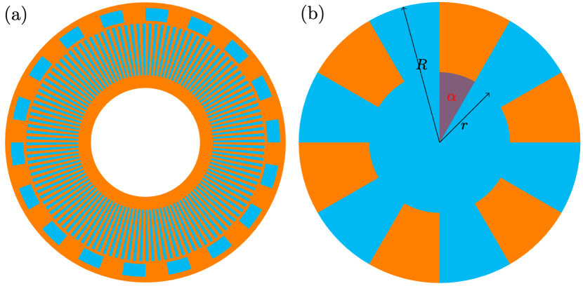
Following the idea developed in Ref. Carlesso et al. (2018b), we explore how to enhance the CSL effect in this purely rotational case by optimizing the shape and the mass density distribution of an hypothetical test mass. The choice of the shape is inspired by the disk used as a torsion balance reported in the experiment in Ref. Lee et al. (2020), which is depicted in Fig. 1(a). The equations of motion of the pendulum we are investigating Carlesso et al. (2016):

$$\dfrac{\operatorname{d}\!\hat{\theta}}{\operatorname{d}\!t}=\frac{\hat{L}}{I}, \dfrac{\operatorname{d}\!\hat{L}}{\operatorname{d}\!t}=-I\omega_{0}^{2}\hat{\theta}-\gamma\hat{L}+\hat{\tau}_{\text{th}}+\hat{\tau}_{\text{\tiny CSL}},$$ (3)

where $\omega_{0}$, $\gamma$, and $I$ are, respectively, the resonance frequency of the torsion balance, the damping of the resonator, and the moment of inertia of the system; $\tau_{\text{th}}$ and $\tau_{\text{\tiny CSL}}$ are the thermal and the CSL stochastic torques. A complete treatment of the problem should consider extra noise terms due to the measurement. However, we take a conservative approach, and assume that all non-thermal noises are caused by CSL. Accounting for other noises can only improve the bounds on the CSL parameters.

Once the correlation functions of the two torques are evaluated, one can derive the thermal and CSL contribution to the Density Noise Spectrum (DNS), whose form is $S_{\tau}(\omega)=\int_{-\infty}^{\infty}\operatorname{d}\!s\,e^{-i\omega s}\mathbb{E}[\langle\hat{\tau}(t)\hat{\tau}(t+s)\rangle]$, where $\mathbb{E}\left[...\right]$ represents the average over the collapse and on the thermal noise, while $\langle...\rangle$ the standard quantum average. A common experimental design involves monitoring the position or the rotation of the system and then determining the force exerted on it, expressing it in terms of the DNS. In the case of a mass with cylindrical symmetry rotating around its axis, the CSL contribution to the torque DNS has the following expression (see Appendix A):

$$S_{\text{\tiny CSL}}(\omega)=\frac{\lambda\hbar^{2}}{4m_{0}^{2}r_{\text{\tiny C}}^{4}}P\times Y,$$ (4)

with

$$Y=\int_{-h/2}^{h/2}\operatorname{d}\!y\int_{-h/2}^{h/2}\operatorname{d}\!y^{\prime}e^{-\frac{(y-y^{\prime})^{2}}{4r_{\text{\tiny C}}^{2}}},$$ (5)

$$P=\int_{0}^{\infty}\operatorname{d}\!r_{\perp}\int_{0}^{\infty}\operatorname{d}\!r^{\prime}_{\perp}r^{2}_{\perp}r^{\prime 2}_{\perp}e^{-\frac{r_{\perp}^{2}+r_{\perp}^{\prime 2}}{4r_{\text{\tiny C}}^{2}}}A(r_{\perp},r_{\perp}^{\prime}),$$

where the integrals are expressed in term of the cylindrical coordinates $\left(r_{\perp},\theta,y\right)$, with $r_{\perp}$ and $\theta$ determining the points of the plane represented in Fig. 1 and $y$ the perpendicular direction. Moreover, we assume a mass distribution of the form $\varrho\left(r_{\perp},\theta,y\right)=H(h/2-y)H(y-h/2)\varrho_{P}(r_{\perp},\theta)$ expressed in terms of the Heaviside function $H$, with $h$ being the thickness of the cylinder. Finally, we define

$$A(r_{\perp},r_{\perp}^{\prime})=\int_{0}^{2\pi}\operatorname{d}\!\theta\int_{0}^{2\pi}\operatorname{d}\!\theta^{\prime}\varrho_{P}(r_{\perp},\theta)\varrho_{P}(r^{\prime}_{\perp},\theta^{\prime})\times$$ (6)

$$\times\left(2r_{\text{\tiny C}}^{2}\cos(\theta-\theta^{\prime})-r_{\perp}r_{\perp}^{\prime}\sin^{2}(\theta-\theta^{\prime})\right)e^{-\frac{2r_{\perp}r_{\perp}^{\prime}\cos(\theta-\theta^{\prime})}{4r_{\text{\tiny C}}^{2}}}\;,$$

which explicitly accounts for the angular and radial mass distribution. To derive a bound, we compare the contribution to the spectral density due to the CSL $S_{\text{\tiny CSL}}(\omega)$ to the one due to thermal fluctuation, which reads $S_{\text{th}}(\omega)=4k_{\text{\tiny B}}T\gamma I$. The bound is found by imposing $S_{\text{\tiny CSL}}(\omega)\leq S_{\text{th}}(\omega)$, this is a conservative approach in which we assume that the CSL contribution is responsible at most for the entire thermal contribution to the DNS. If we modify the mass density of the system without altering the moment of inertia $I$, then $S_{\text{th}}$ remains constant. For this reason most of the analysis here is performed by keeping $I$ fixed.

III A simplified model

The following analysis aims at enhancing the CSL effect by introducing a periodic mass density in the angular variable as depicted in Fig. 1(b). Here, we study a simplified model, where the system is composed by a single annulus with a periodic mass density. This is a case with fewer parameters with respect to that in Fig. 1(a), which refers to the experiment in Ref. Lee et al. (2020).

Figure 1: Top view of the mass density configurations. The orange region has density $\varrho+\Delta\varrho$ and the cyan one has density $\varrho$. Panel (a) shows the actual configuration used in Lee et al. (2020). Panel (b) represents a simplified configuration; the angle subtended by the orange sectors is denoted by $\alpha$, while $r$ and $R$ represent the inner and the outer radii of the annulus with periodic mass density.

To evaluate the torque DNS, we introduce the following mass density function for this configuration:

$$\varrho_{P}(r_{\perp},\theta)=H(R-r_{\perp})\bigg{[}\varrho H(r_{\perp})+\Delta\varrho H(r_{\perp}-r)$$ (7)

$$\times\sum_{j=0}^{n-1}H\left(\theta-\frac{2j\pi}{n}\right)H\left(\frac{2j\pi}{n}+\alpha-\theta\right)\bigg{]},$$

where $\varrho$ is the mass density of the lighter material (shown in cyan in Fig. 1), $\Delta\varrho>0$ is the difference of mass densities between the two materials, $2n$ is the number of sectors in which the annulus is divided, $\alpha\in\left[0,2\pi/n\right]$ is the angle subtended by a orange sector, $r$ and $R$ are respectively the inner and outer radii. We show in Appendix A that the first term in parenthesis, corresponding to the homogeneous cylinder at the centre of the annulus, does not contribute to the CSL effect. Conversely, the second one does. Thus according to Eq. (6), the effect scales with the square of the density difference between the materials $\Delta\rho$. Moreover, in the configuration just described, Eq. (6) can be evaluated analitically leading to the following expression

Figure 2: Upper Panels: comparison of the values of $P$ for different mass density functions of the simplified model for (a) $r_{\text{\tiny C}}=10^{-4}\,\mathrm{m}$ and (b) $r_{\text{\tiny C}}=10^{-7}\,\mathrm{m}$ . The values of $n$ taken into consideration are $n=4$ (blue lines), $n=10$ (red lines), $n=20$ (green lines), $n=100$ (orange lines). The orange line in panel (a) drops at $\alpha=2\pi/100$, which corresponds to the homogeneous limit. The solid and dashed lines represent the cases in which $\epsilon=2$ and $\epsilon=20$, respectively. The moment of inertia is kept fixed at $I=9\times 10^{-6}\,\mathrm{kg}\,\mathrm{m^{2}}$ by changing the value of $r$. The thickness of the cylinder is kept fixed at $h=10^{-4}\,\mathrm{m}$. Lower panels: comparison of the values of $P\times Y$ for different mass density functions of the simplified model for (c) $r_{\text{\tiny C}}=10^{-4}\,\mathrm{m}$ and (d) $r_{\text{\tiny C}}=10^{-7}\,\mathrm{m}$. The parameter $h$ is varying while $\epsilon=2$ and $I=9\times 10^{-6}\,\mathrm{kg}\,\mathrm{m^{2}}$ are kept fixed. In panels (b) and (d) we only analysed the case with $n=4$ since for $r_{\text{\tiny C}}=10^{-7}\mathrm{m}$ the effect of the model is much smaller than the case of $r_{\text{\tiny C}}=10^{-4}$ m, and it is not worth a more detailed analysis.

$$A(r_{\perp},r_{\perp}^{\prime})= \frac{32r_{\text{\tiny C}}^{4}\Delta\varrho^{2}}{r_{\perp}r_{\perp}^{\prime}}\prod_{r_{x}=r^{\prime}_{\perp},r_{\perp}}H(r_{x}-r)H(R-r_{x})$$ (8)

$$\times\sum_{j=0}^{\infty}I_{jn}\left(\frac{r_{\perp}r^{\prime}_{\perp}}{2r_{\text{\tiny C}}^{2}}\right)n^{2}\sin^{2}\left(\frac{\alpha jn}{2}\right),$$

where $I_{\sigma}(x)$ are the modified Bessel function of the first kind of order $\sigma=j\times n$. We note that $A$ is zero in $\alpha=0$ and $\alpha=2\pi/n$, since these value correspond to a homogeneous mass density configuration.

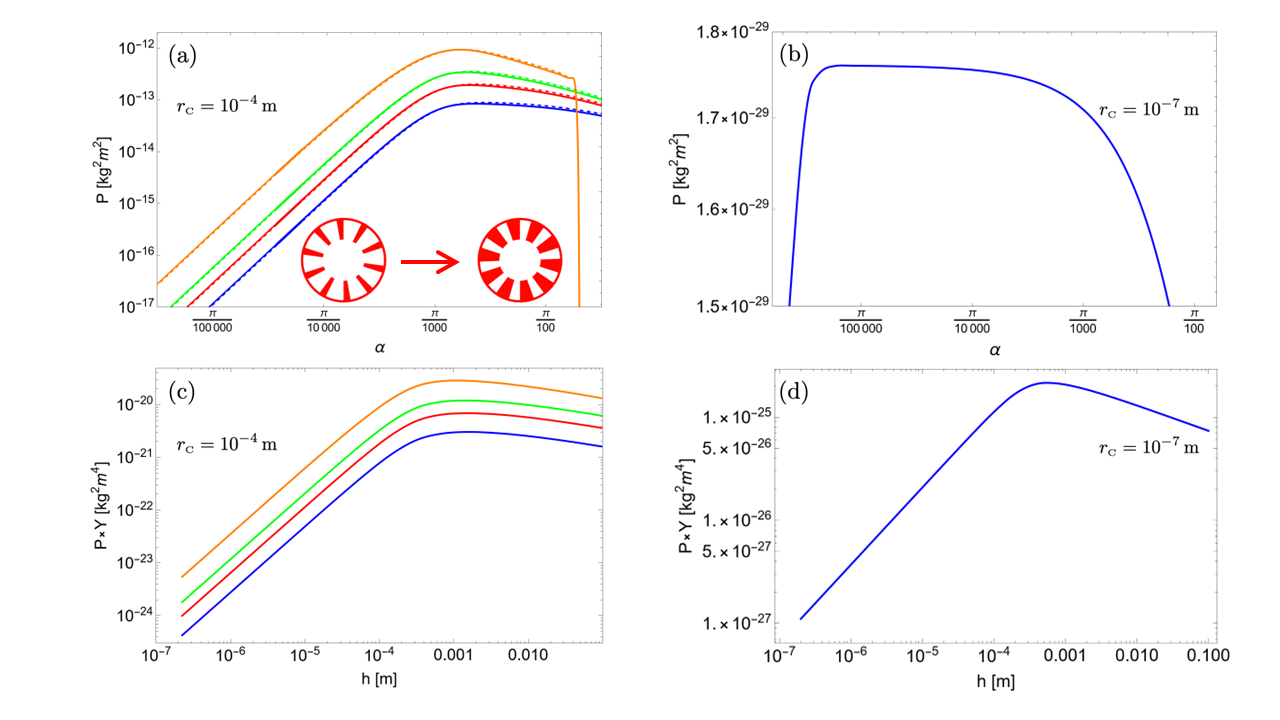
We can start our numerical analysis of $Y$ and $P$ noting that, once the value of the moment of inertia $I$ and the material densities are fixed, $P$ depends on: the angle $\alpha$, the number $n$ of heavier (orange) sectors, the inner ($r$) and outer ($R$) radii and the height ($h$). We consider the values $r_{\text{\tiny C}}=10^{-4}\,\text{m}$ and $r_{\text{\tiny C}}=10^{-7}\,\text{m}$ for reference, and compute $P$ for $n=4,10,20$ and $\epsilon={R}/{r}=2$ and $20$ by varying $\alpha$ in the interval $[0,2\pi/n]$. To keep the value of $I$ fixed, we change the value of $r$ as a function of the different values assumed by $n$, $\alpha$ and $\epsilon$, while keeping $h$ fixed. Under this assumption, the value of $Y$ is constant.

Figure 2 shows the dependence of $P$ from $\alpha$ for $r_{\text{\tiny C}}\simeq 10^{-4}\,\mathrm{m}$ and $r_{\text{\tiny C}}\simeq 10^{-7}\,\mathrm{m}$. The optimal value of $\alpha$ does not depend strongly on the value of $n$, while it does on the value of $r_{\text{\tiny C}}$. This behaviour is the same that has been noticed in Ref. Carlesso et al. (2018b). Indeed, in this case the maximum of the CSL effect occurs when $r_{\text{\tiny C}}$ and the arc length subtended by the $\alpha$ sector are similar. Panel (a) shows that there is an enhancement of the CSL effect on $P$ for $r_{\text{\tiny C}}=10^{-4}\,$m when increasing the number $n$ of sectors. The dependence on $\epsilon$ seems less impactfull: the dashed line ($\epsilon=20$) and the solid line ($\epsilon=2$) almost completely overlap for every $n$. Finally, it is important to note that the orange curve, corresponding to the annulus with $n=100$ orange sectors, goes to zero for $\alpha\rightarrow 2\pi/100$. This is expected, since it corresponds to an homogeneous mass configuration. Panel (b) shows the behaviour of $P$ for $r_{\text{\tiny C}}=10^{-7}\,\mathrm{m}$: the constraints imposed on the geometry (the choice of the value of $r$) produce a weaker CSL effect in comparison with that shown in panel (a).

In the following numerical analysis, we fix the values of $r_{\text{\tiny C}}$, $\epsilon$, $I$ and therefore $\alpha$ to their optimal values, based on the choice of $r_{\text{\tiny C}}$. These are shown in Tab. 1. We then evaluate $P\times Y$ by letting $h$ and $n$ vary, and at the same time we change $r$ to maintain $I$ constant. This analysis gives us the optimal value of $h$ from panel (c) and (d) of Fig. 2 in correspondence of the two values of $r_{\text{\tiny C}}$ here considered.

$r_{\text{\tiny C}}\,[\mathrm{m}]$	$\epsilon$	$I\,[\mathrm{kg}\,\mathrm{m^{2}}]$	$\alpha$	$h\,[\mathrm{m}]$	n
$10^{-4}$	$2$	$9\times 10^{-6}$	$5\times 10^{-3}$	$10^{-3}$	100
$10^{-7}$	$2$	$9\times 10^{-6}$	$3\times 10^{-5}$	$6\times 10^{-3}$	4

Table 1: Optimised values of the parameters obtained from the numerical analysis for the simplified model.

$h\,[\mathrm{m}]$	$I\,[\mathrm{kg/m^{3}}]$	$\gamma\,[\mathrm{Hz}]$	$T\,[\mathrm{K}]$	$\rho\,[\mathrm{kg/m^{3}}]$	$\Delta\rho\,[\mathrm{kg/m^{3}}]$
$5.4\times 10^{-5}$	$9.2\times 10^{-6}$	$4.6\times 10^{-6}$	$273$	$1.2\times 10^{3}$	$19.3\times 10^{3}$
$r\,[\mathrm{m}]$	$r_{120}\,[\mathrm{m}]$	$R_{120}\,[\mathrm{m}]$	$r_{18}\,[\mathrm{m}]$	$R_{18}\,[\mathrm{m}]$	$R\,[\mathrm{m}]$
$1.05\times 10^{-2}$	$1.30\times 10^{-2}$	$2.30\times 10^{-2}$	$2.35\times 10^{-2}$	$2.60\times 10^{-2}$	$2.70\times 10^{-2}$

Table 2: Parameters of the setup in Lee et al. (2020) (see also Fig.1): the height $h$, momentum of inertia $I$, damping of the resonator $\gamma$, temperature $T$, mass density $\rho$, mass density difference $\Delta\rho$, and the radii (from the most inner to the most outer): internal radius $r$, for the annulus with 120 sectors internal radius $r_{120}$ and external $R_{120}$, for the annulus with 18 sectors internal radius $r_{18}$ and external $R_{18}$, external radius $R$.

In summary, from Fig. 2 it is possible to identify the optimal values of $\alpha$ and $h$ in order to enhance the bound at $r_{\text{\tiny C}}=10^{-4}\,\mathrm{m}$ and $r_{\text{\tiny C}}=10^{-7}\,\mathrm{m}$. Fixing these parameters to their optimal value [cf. Tab. 1] for $r_{\text{\tiny C}}=10^{-4}\,\mathrm{m}$, we derive the corresponding bound, which is reported in Fig. 3 (black line).

IV Comparison with experimental data

The experiment Lee et al. (2020) that inspired this analysis was designed to test gravity over short distances to find possible violations of the gravitational inverse square law. In particular, the experiment was used to constrain a possible additional Yukawa interaction to the Newtonian potential of the form: $V(r)=V_{N}(r)[1+a\exp(-r/\ell)]$, where $V_{N}(r)$ is the Newtonian potential, and $a$ and $\ell$ are the free parameters to be tested. The mass used in the experiment is represented in Fig. 1(a).

The disk considered in the experiment consist of two concentric annuli; we then have extended the analysis presented in the previous section to more then one annulus. In this way we will show that it is possible to enhance the CSL effect for different values of $r_{\text{\tiny C}}$ simultaneously. In the case of two concentric annuli with different angular periodicity (internal annulus with $n$ orange sectors, external annulus with $m$ orange sectors [cf. Fig. 1(a)]) Eq. (6) takes the following form:

$$A(r_{\perp},r_{\perp}^{\prime},m,n)=\frac{32r_{\text{\tiny C}}^{4}}{r_{\perp}r^{\prime}_{\perp}}\Delta\varrho^{2}\sum_{k=1}^{\infty}I_{k}\left(\frac{r_{\perp}r^{\prime}_{\perp}}{2r_{\text{\tiny C}}^{2}}\right)\bigg{[}\sum_{\nu=n,m}\nu^{2}\sum_{h=0}^{\infty}\delta_{k,(2h+1)\nu}\prod_{r_{x}=r^{\prime}_{\perp},r_{\perp}}H(r_{x}-r_{\nu})H(R_{\nu}-r_{x})+$$ (9)

$$+mnH(r^{\prime}_{\perp}-r_{n})H(R_{n}-r^{\prime}_{\perp})H(r_{\perp}-r_{m})H(R_{m}-r_{\perp})\bigg{(}\sum_{h=0}^{\infty}\sum_{h^{\prime}=0}^{\infty}\delta_{k,(2h+1)m}\delta_{k,(2h^{\prime}+1)n}\bigg{)}\bigg{]},$$

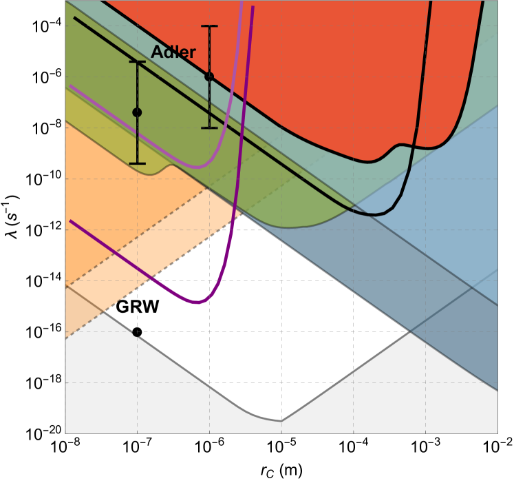
where $r_{\nu}$ and $R_{\nu}$ are respectively the inner and outer radii of the $\nu$-th annulus, with $\nu=n$ and $\nu=m$ indicating the internal and external annulus respectively. We recall that the terms representing an homogeneous mass density do not contribute to the effect. In the second line of Eq. (9) a mixed term is present, this is where both the inner and outer annuli parameters appear. It vanishes if $n$ and $m$ satisfy the condition $(2k+1)m\not=(2k^{\prime}+1)n,\ \forall k\in\mathbb{N},\forall k^{\prime}\in\mathbb{N}$. In our case, we have $n=120$ and $m=18$ that satisfy this condition, thus only the first line of Eq. (9) contributes. Now we take the experimental results reported in Ref. Lee et al. (2020) to set an upper bound on the parameters of the CSL model as discussed in Sec. II. In doing this, we consider the frequency region between $2\times 10^{-3}\,$Hz and $10^{-1}\,$Hz (the resonant frequency is $\omega_{0}=1.8\times 10^{-2}\,$Hz) of the experimental spectrum in which the main noise is the thermal one. The parameters characterizing the test mass are summarised in Tab. 2. The corresponding bound is shown in Fig. 3 with the red area; it has two local minima reflecting the two different periodicities.

Figure 3: Exclusion plot for the CSL parameters $\lambda$ and $r_{\text{\tiny C}}$ from rotational tests, compared with the existing experimental bounds. The red area represent the region excluded by the experiment in Ref. Lee et al. (2020). The black line is the hypothetical upper bound derived by optimising the geometry of the simplified model for $r_{\text{\tiny C}}\simeq 10^{-4}\,\mathrm{m}$ and $T=273\;\mathrm{K}$. The light purple and the dark purple lines refers to the hypothetical bounds derived by optimizing the geometry of the simplified model for $r_{\text{\tiny C}}\simeq 10^{-6}\,\mathrm{m}$ at different temperatures $T$, respectively $T=273\,\mathrm{K}$ and $T=1\,\mathrm{mK}$. These upper bound are compared with the coloured areas corresponding to regions already excluded experimentally. The green regions refer to cantilever-based experiments with multilayer structures Vinante et al. (2020a). The blue areas to gravitational wave detectors Carlesso et al. (2016, 2018c); Helou et al. (2017): LIGO (light blue) and LISA Pathfinder (dark blue). The orange areas delimited by the dashed lines are from spontaneous $\mathrm{X}$-ray emission tests: the darker one is derived in Ref. Donadi et al. (2021) and the lighter one is derived in Majorana Arnquist et al. (2022). The light grey area is excluded from the requirement that macroscopic superpositions do not persist in time Toroš et al. (2017). The white area is yet to be explored.

V Discussion and future perspective

In the relevant range of values of $r_{\text{\tiny C}}$, the bound derived from the experiment in Ref. Lee et al. (2020) is comparable to that excluded by the much more sophisticated experiment LIGO Carlesso et al. (2016). The considered experiment was not designed to test the CSL model, therefore it is possible to optimize the geometry of the system to improve even further the bound in regions of the parameters plot yet to be explored. For example, in the simplified model, it is possible to derive a bound with its minimum at $r_{\text{\tiny C}}=10^{-6}\,\mathrm{m}$ by choosing the parameters as follows: $r=10^{-5}\,\mathrm{m}$, $R=2\times 10^{-4}\,\mathrm{m}$, $n=300$, $\alpha=\pi/n$, $h=10^{-3}\,\mathrm{m}$ . If we assume $T=273\,\mathrm{K}$, we obtain the bound represented with a light purple line. However, by taking $T\simeq 1\,\mathrm{mK}$ we obtain a stronger bound (dark purple line), which allows to explore a new region at $r_{\text{\tiny C}}=10^{-6}\,\mathrm{m}$. This comes with the assumptions that it is possible to realize a test mass with the above parameters, and that thermalises at $1\,\mathrm{mK}$. Experiments around this temperature have already been carried out Vinante et al. (2020b).

To conclude, we summarise the main properties of the proposed technique: a geometry with concentric annuli is capable of simultaneously probing multiple regions of the parameter space. The effect of the model is maximum approximately when the arc length subtended by the sectors is comparable to $r_{\text{\tiny C}}$ (this is verifiable analytically for a simple case discussed in Appendix B). Conversely, there is no advantage into applying this technique to test $r_{\text{\tiny C}}$ bigger than the system’s dimension. Indeed, the effect fades rapidly as $r_{\text{\tiny C}}$ increases. Our analysis shows that in principle this technique can offer competitive bounds in the same region ($10^{-7}\;\mathrm{m}<r_{\text{\tiny C}}<10^{-6}\;\mathrm{m}$) as that touched by X-ray detection experiments (orange areas in Fig. 3). However, the latter experiments, in contrast to mechanical oscillators, target the high frequency region of the CSL noise spectrum and as such are much more sensible to changes in noise, for example based on the introduction of a cutoff Adler et al. (2013); Donadi et al. (2014); Carlesso et al. (2018a). In such a case, the bounds highlighted in orange loose strength and the purple bound presented here becomes the dominant one.

Appendix A CSL Torque from the Master Equation

We derive the CSL torque $\tau_{\text{\tiny CSL}}$ starting from the master equation (1). This dynamics can be reproduced by a standard Schrödinger equation with an additional stochastic potential of the form Carlesso et al. (2016):

$$\hat{V}_{\text{\tiny CSL}}(t)=-\frac{\hbar\sqrt{\lambda}}{\pi^{3/4}r_{\text{\tiny C}}^{3/2}m_{0}^{2}}\int\operatorname{d}\!\boldsymbol{z}\hat{M}(\boldsymbol{z})w(\boldsymbol{z},t),$$ (10)

where $w(\boldsymbol{z},t)$ is a collection of white noises (one for each point of space $\boldsymbol{z}$) with $\mathbb{E}[w(\boldsymbol{z},t)]=0$ and $\mathbb{E}[w(\boldsymbol{z},t)w(\boldsymbol{y},s)]=\delta(t-s)\delta^{(3)}(\boldsymbol{z}-\boldsymbol{y})$. Such a stochastic potential acts on the $n$-th particles of the system as a stochastic force:

$$\boldsymbol{\hat{F}}_{n}=\frac{i}{\hbar}[\hat{V}_{\text{\tiny CSL}},\boldsymbol{\hat{p}}_{n}].$$ (11)

Then the position operator can be written as $\boldsymbol{\hat{q}}_{n}=\boldsymbol{q}^{(0)}_{n}+\Delta\boldsymbol{\hat{q}}_{n}$, where $\boldsymbol{q}^{(0)}_{n}$ is the classical equilibrium position of the $\alpha$-th nucleon and $\Delta\boldsymbol{\hat{q}}_{n}$ quantifies the quantum displacement of the $n$-th nucleon with respect to its classical equilibrium position. Now assuming that we are dealing with a rigid body and that the quantum fluctuations are small with respect to $r_{\text{\tiny C}}$, we can Taylor expand the mass density:

$$\hat{M}(\boldsymbol{z})=M_{0}(\boldsymbol{z})+\sum_{n}r_{\text{\tiny C}}^{-2}\int\operatorname{d}\!\boldsymbol{x}\,\varrho(\boldsymbol{x})\exp\left(-(\boldsymbol{z}-\boldsymbol{x})^{2}/\left(2r_{\text{\tiny C}}^{2}\right)\right)(\boldsymbol{z}-\boldsymbol{x})\cdot\Delta\hat{\boldsymbol{q}}_{n},$$ (12)

where $M_{0}(z)$ is a classical function whose form is not important. Thus, Eq. (11) becomes:

$$\boldsymbol{F}_{n}(t)=\frac{\hbar\sqrt{\lambda}}{\pi^{3/4}m_{0}}\int\frac{\operatorname{d}\!\boldsymbol{z}}{r_{\text{\tiny C}}^{7/2}}e^{-\frac{(\boldsymbol{z}-\boldsymbol{q}^{(0)}_{n})^{2}}{2r_{\text{\tiny C}}^{2}}}(\boldsymbol{z}-\boldsymbol{q}^{(0)}_{n})w(\boldsymbol{z},t).$$ (13)

Since the geometry of the system studied is cylindrical, as depicted in Fig. 1, it is easier to handle the problem using cylindrical coordinates, defined as $y$, $r_{\perp}=\sqrt{x^{2}+z^{2}}$ and $\theta=\arctan(x/z)$. By using the tangent component of the force $F_{\theta}(\boldsymbol{x},t)=\boldsymbol{F}(\boldsymbol{x},t)\cdot\boldsymbol{e}_{\theta}$, we can evaluate the torque along $y$ acting on the whole system:

$$\tau_{\text{\tiny CSL}}\left(t\right)=\int\,\operatorname{d}\!r_{\perp}\operatorname{d}\!\theta\operatorname{d}\!y\;r_{\perp}^{2}\,F_{\theta}(\boldsymbol{x},t).$$ (14)

Starting from the correlation function for $F_{\theta}(\boldsymbol{x},t)$

$$\mathbb{E}[F_{\theta}(\boldsymbol{x},t)\,F_{\theta}(\boldsymbol{x}^{\prime},s)]=\frac{\lambda\hbar^{2}}{4m_{0}^{2}r_{\text{\tiny C}}^{4}}\left(2r_{\text{\tiny C}}^{2}\cos(\theta-\theta^{\prime})-r_{\perp}r_{\perp}^{\prime}\sin^{2}(\theta-\theta^{\prime})\right)\varrho(\boldsymbol{x})\varrho(\boldsymbol{x}^{\prime})\times$$ (15)

$$\times\exp\left(-\frac{r_{\perp}^{2}-2r_{\perp}r_{\perp}^{\prime}\cos(\theta-\theta^{\prime})+r_{\perp}^{\prime 2}+(y-y^{\prime})^{2}}{4r_{\text{\tiny C}}^{2}}\right)\delta(t-s),$$

we can evaluate the correlation function for $\tau_{\text{\tiny CSL}}$ as:

$$\mathbb{E}\left[\tau_{\text{\tiny CSL}}(t)\tau_{\text{\tiny CSL}}(s)\right]=\int\,\operatorname{d}\!r_{\perp}\operatorname{d}\!\theta\operatorname{d}\!y\;\int\,\operatorname{d}\!r^{\prime}_{\perp}\operatorname{d}\!\theta^{\prime}\operatorname{d}\!y^{\prime}\;r^{2}_{\perp}r^{\prime 2}_{\perp}\;\mathbb{E}[\,F_{\theta}(\boldsymbol{x},t)\,F_{\theta}(\boldsymbol{x}^{\prime},s)].$$ (16)

Finally, one obtains the DNS via:

$$S_{\text{\tiny CSL}}(\omega)=\int_{-\infty}^{\infty}\operatorname{d}\!s\,e^{-i\omega s}\mathbb{E}\left[\tau_{\text{\tiny CSL}}(t)\tau_{\text{\tiny CSL}}(t+s)\right].$$ (17)

Now, we analyze the case in which the mass density is independent from $\theta$, i.e. rotationally homogeneous. We consider only the radial and angular part of the previous integral. We recall the following known identities:

$$\int_{0}^{2\pi}\operatorname{d}\!\theta\cos(\theta-\theta^{\prime})\exp\left(\frac{r_{\perp}r_{\perp}^{\prime}\cos(\theta-\theta^{\prime})}{2r_{\text{\tiny C}}^{2}}\right)=2\pi I_{1}\left(\frac{r_{\perp}r_{\perp}^{\prime}}{2r_{\text{\tiny C}}^{2}}\right)$$ (18)

and

$$\int_{0}^{2\pi}\operatorname{d}\!\theta\sin^{2}(\theta-\theta^{\prime})\exp\left(\frac{r_{\perp}r_{\perp}^{\prime}\cos(\theta-\theta^{\prime})}{2r_{\text{\tiny C}}^{2}}\right)=2\pi\frac{I_{1}\left(\frac{r_{\perp}r_{\perp}^{\prime}}{2r_{\text{\tiny C}}^{2}}\right)}{\frac{r_{\perp}r_{\perp}^{\prime}}{2r_{\text{\tiny C}}^{2}}}.$$ (19)

where $I_{1}$ is the modified Bessel function of the first kind. Finally, by replacing Eq. (18) and Eq. (19) in Eq. (16) one finds that the CSL effect vanishes. This means that CSL has no effect on rotations of a rotationally homogeneous system.

Appendix B Study of a simple system for understanding the CSL amplification mechanism

To better understand the relation between the size of the test mass and the maximization of the CSL effects, we consider the simple example of a half cylinder of radius $R$. In this case the expression in Eq. (6) takes the simple form:

$$A(r_{\perp},r_{\perp}^{\prime})=32r_{\text{\tiny C}}^{4}\Delta\varrho^{2}\sum_{j=0}^{\infty}I_{2j+1}\left(\frac{r_{\perp}r^{\prime}_{\perp}}{2r_{\text{\tiny C}}^{2}}\right)\prod_{r_{x}=r^{\prime}_{\perp},r_{\perp}}\frac{H(R-r_{x})}{r_{x}}=16r_{\text{\tiny C}}^{4}\Delta\varrho^{2}\sinh\left(\frac{r_{\perp}r^{\prime}_{\perp}}{2r_{\text{\tiny C}}^{2}}\right)\prod_{r_{x}=r^{\prime}_{\perp},r_{\perp}}\frac{H(R-r_{x})}{r_{x}},$$ (20)

and the corresponding form of $P$ becomes:

$$P=16r_{\text{\tiny C}}^{4}\Delta\varrho^{2}\int_{0}^{R}\operatorname{d}\!r_{\perp}\int_{0}^{R}\operatorname{d}\!r^{\prime}_{\perp}r_{\perp}r^{\prime}_{\perp}e^{-\frac{r_{\perp}^{2}+r_{\perp}^{\prime 2}}{4r_{\text{\tiny C}}^{2}}}\sinh\left(\frac{r_{\perp}r^{\prime}_{\perp}}{2r_{\text{\tiny C}}^{2}}\right).$$ (21)

Then, we equate the CSL contribution to the thermal noise, which depends on the moment of inertia of the half cylinder: $I=\frac{\pi}{4}h\varrho R^{4}$. It follows that the dependence of the corresponding $\lambda$ can be expressed in terms of $\lambda\propto(F(R/r_{\text{\tiny C}}))^{-1}$ where

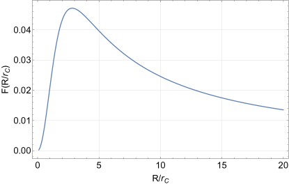
$$F\left(\frac{R}{r_{\text{\tiny C}}}\right)=\frac{2-3\left(\frac{R}{r_{\text{\tiny C}}}\right)^{2}+e^{-\left(\frac{R}{r_{\text{\tiny C}}}\right)^{2}}\left(-2+\left(\frac{R}{r_{\text{\tiny C}}}\right)^{2}\right)+\sqrt{\pi}\left(\frac{R}{r_{\text{\tiny C}}}\right)^{3}\mathrm{erf}\left(\frac{R}{r_{\text{\tiny C}}}\right)}{\left(\frac{R}{r_{\text{\tiny C}}}\right)^{4}}.$$ (22)

From the plot in Fig. 4 we can see that the maximum of the term in parenthesis (which gives the optimized value of $R/r_{\text{\tiny C}}$ in order to have a stronger bound for $\lambda$) is for values of $R/r_{\text{\tiny C}}\simeq 3$.

Figure 4: Dependence of $F$ in Eq. (21) on the dimensionless ratio between the radius of the cylinder and the CSL parameter $r_{\text{\tiny C}}$

Appendix C Colored CSL Evaluation

We can generalise our calculation to the colored version of the CSL model (the quantities relative to this model contain the label C), in which $\mathbb{E}[w_{\text{\tiny C}}(\boldsymbol{z},t)w_{\text{\tiny C}}(\boldsymbol{y},s)]=f(t-s)\delta^{(3)}(\boldsymbol{z}-\boldsymbol{y})$, where $f(t)$ is a correlation function with colored spectrum. By taking $f(t)=\delta(t)$ one recovers the standard CSL model. In this case the correlation function for $F^{\text{\tiny C}}_{\theta}(\boldsymbol{x},t)$ is the same as in Eq. (15) with $f(t-s)$ substituting $\delta(t-s)$. As already derived in Ref. Carlesso et al. (2018d), the colored density noise spectrum can be defined in terms of the white one, which is shown in Eq. (4):

$$S^{\text{\tiny C}}_{\text{\tiny CSL}}(\omega)=\tilde{f}(\omega)\times S_{\text{\tiny CSL}}(\omega).$$ (23)

where $\tilde{f}(\omega)$ is the Fourier transform of $f(t)$. We consider a exponential correlation function $f$, which is characteristic of many physical processes, as already done Ref. Bassi and Ferialdi (2009):

$$f(t-s)=\frac{\Omega_{\text{\tiny C}}}{2}e^{-\Omega_{\text{\tiny C}}|t-s|},$$ (24)

with correlation time $\Omega_{\text{\tiny C}}^{-1}$; by doing this we introduce a cutoff in the frequency domain. Correspondingly we obtain the following DNS:

$$S^{\text{\tiny C}}_{\text{\tiny CSL}}(\omega)=\frac{\Omega^{2}_{\text{\tiny C}}}{\Omega^{2}_{\text{\tiny C}}+\omega^{2}}S_{\text{\tiny CSL}}(\omega).$$ (25)

As long as $\Omega_{\text{\tiny C}}\gg\omega\simeq 10^{-2}\,\mathrm{s^{-1}}$, $S^{\text{\tiny C}}_{\text{\tiny CSL}}(\omega)\simeq S_{\text{\tiny CSL}}(\omega)$, meaning that the results derived in the main text are not affected by the cutoff. For comparison, the bounds on the CSL parameters coming from the spontaneous radiation emission set in Ref. Arnquist et al. (2022) for the Majorana Demonstrator remain valid only for values of the cut-off $\Omega_{\text{\tiny C}}\gg 10^{19}\;\mathrm{s^{-1}}$. As discussed in Carlesso et al. (2018d) a reasonable value for the cutoff frequency is $\Omega_{\text{\tiny C}}\simeq 10^{12}\,$s^-1, which leaves unaffected the bound derived in this work, but suppresses the bound set by radiation emission experiments.

References

- Bassi and Ghirardi (2003) A. Bassi and G. Ghirardi, Physics Reports 379, 257 (2003).
- Bassi et al. (2013) A. Bassi, K. Lochan, S. Satin, T. P. Singh, and H. Ulbricht, Reviews of Modern Physics 85, 471 (2013).
- Carlesso et al. (2022) M. Carlesso, S. Donadi, L. Ferialdi, M. Paternostro, H. Ulbricht, and A. Bassi, Nature Physics 18, 243 (2022).
- Ghirardi et al. (1990) G. C. Ghirardi, P. Pearle, and A. Rimini, Physical Review A 42, 78 (1990).
- Ghirardi et al. (1986) G. C. Ghirardi, A. Rimini, and T. Weber, Physical review D 34, 470 (1986).
- Adler (2007) S. L. Adler, Journal of Physics A: Mathematical and Theoretical 40, 2935 (2007).
- Bahrami et al. (2014) M. Bahrami, M. Paternostro, A. Bassi, and H. Ulbricht, Physical Review Letters 112, 210404 (2014).
- Nimmrichter et al. (2014) S. Nimmrichter, K. Hornberger, and K. Hammerer, Physical review letters 113, 020405 (2014).
- Diósi (2015) L. Diósi, Physical review letters 114, 050403 (2015).
- Donadi et al. (2023) S. Donadi, L. Ferialdi, and A. Bassi, Physical Review Letters 130, 230202 (2023).
- Lee et al. (2020) J. G. Lee, E. G. Adelberger, T. S. Cook, S. M. Fleischer, and B. R. Heckel, Phys. Rev. Lett. 124, 101101 (2020).
- Carlesso et al. (2016) M. Carlesso, A. Bassi, P. Falferi, and A. Vinante, Physical Review D 94, 124036 (2016).
- Carlesso et al. (2018a) M. Carlesso, L. Ferialdi, and A. Bassi, The European Physical Journal D 72 (2018a).
- Arnquist et al. (2022) I. Arnquist, F. Avignone III, A. Barabash, C. Barton, K. Bhimani, E. Blalock, B. Bos, M. Busch, M. Buuck, T. Caldwell, et al., Physical Review Letters 129, 080401 (2022).
- Adler and Bassi (2007) S. L. Adler and A. Bassi, Journal of Physics A: Mathematical and Theoretical 40, 15083 (2007).
- Schrinski et al. (2017) B. Schrinski, B. A. Stickler, and K. Hornberger, JOSA B 34, C1 (2017).
- Carlesso et al. (2018b) M. Carlesso, A. Vinante, and A. Bassi, Physical Review A 98, 022122 (2018b).
- Vinante et al. (2020a) A. Vinante, M. Carlesso, A. Bassi, A. Chiasera, S. Varas, P. Falferi, B. Margesin, R. Mezzena, and H. Ulbricht, Physical Review Letters 125, 100404 (2020a).
- Carlesso et al. (2018c) M. Carlesso, M. Paternostro, H. Ulbricht, A. Vinante, and A. Bassi, New Journal of Physics 20, 083022 (2018c).
- Helou et al. (2017) B. Helou, B. Slagmolen, D. E. McClelland, and Y. Chen, Physical Review D 95, 084054 (2017).
- Donadi et al. (2021) S. Donadi, K. Piscicchia, R. Del Grande, C. Curceanu, M. Laubenstein, and A. Bassi, The European Physical Journal C 81, 1 (2021).
- Toroš et al. (2017) M. Toroš, G. Gasbarri, and A. Bassi, Physics Letters A 381, 3921 (2017).
- Vinante et al. (2020b) A. Vinante, M. Carlesso, A. Bassi, A. Chiasera, S. Varas, P. Falferi, B. Margesin, R. Mezzena, and H. Ulbricht, Physical Review Letters 125 (2020b).
- Adler et al. (2013) S. L. Adler, A. Bassi, and S. Donadi, Journal of Physics A: Mathematical and Theoretical 46, 245304 (2013).
- Donadi et al. (2014) S. Donadi, D.-A. Deckert, and A. Bassi, Annals of Physics 340, 70 (2014).
- Carlesso et al. (2018d) M. Carlesso, L. Ferialdi, and A. Bassi, The European Physical Journal D 72, 1 (2018d).
- Bassi and Ferialdi (2009) A. Bassi and L. Ferialdi, Physical Review A 80, 012116 (2009).