Not all distributional shifts are equal:
Fine-grained robust conformal inference

Abstract

We introduce a fine-grained framework for uncertainty quantification of predictive models under distributional shifts. This framework distinguishes the shift in covariate distributions from that in the conditional relationship between the outcome ($Y$) and the covariates ($X$). We propose to reweight the training samples to adjust for an identifiable covariate shift while protecting against worst-case conditional distribution shift bounded in an $f$-divergence ball. Based on ideas from conformal inference and distributionally robust learning, we present an algorithm that outputs (approximately) valid and efficient prediction intervals in the presence of distributional shifts. As a use case, we apply the framework to sensitivity analysis of individual treatment effects with hidden confounding. The proposed methods are evaluated in simulation studies and three real data applications, demonstrating superior robustness and efficiency compared with existing benchmarks.

1 Introduction

It has been widely observed that the performance of predictive models falls short of expectation when generalized to a population whose distribution differs from that of the training data (see e.g., Recht et al., (2019); Miller et al., (2020); Wong et al., (2021); Namkoong et al., (2023); Liu et al., (2023) and the references therein). As predictive models are increasingly employed in high-stakes settings, it is imperative to accompany the predicted outcomes with calibrated uncertainty quantification when deploying a model to new environments. A widely adopted approach to uncertainty quantification is to provide a prediction set that contains the true outcome with high probability. The prediction set informs the confidence we have in the predicted outcome.

Among the tools for constructing prediction sets, conformal prediction (CP) (Vovk et al.,, 2005) is an attractive framework that generates valid prediction sets that are guaranteed to include the true outcome with pre-specified probability. The validity of CP holds for any predictive model, as long as the training and test data are exchangeable, e.g., when they are identically independently distributed (i.i.d.). In the presence of distributional shifts, however, the exchangeability/i.i.d. assumption breaks, and CP no longer delivers valid prediction sets. To address this challenge, prior work (Cauchois et al.,, 2023) proposes a robust CP method that outputs prediction sets that are valid when the target distribution ranges within a neighborhood of the training distribution. To be more specific, let $X\in{\mathcal{X}}$ denote the covariates and $Y\in{\mathcal{Y}}$ the outcome/response. Consider a training set of $n$ samples $(X_{i},Y_{i})\stackrel{{\scriptstyle\text{i.i.d.}}}{{\sim}}P_{X,Y}$ and an independent test unit $(X_{n+1},Y_{n+1})\sim Q_{X,Y}$, where we only get to observe $X_{n+1}$ and wish to predict $Y_{n+1}$. Cauchois et al., (2023) assumes that the $f$-divergence between $Q_{X,Y}$ and $P_{X,Y}$ is bounded by a parameter $\rho$, and provides prediction sets that ensure guarantees even for the worst-case $Q_{X,Y}$.

The method of Cauchois et al., (2023) provides robustness against the worst-case joint distributional shift of $(X,Y)$, but no distinction is made between the covariate shift and the conditional distributional shift. As pointed out by a recent line of research, different types of distributional shifts appear in different tasks and result in different consequences (Mu et al.,, 2022; Namkoong et al.,, 2023; Jin et al., 2023a, ; Liu et al.,, 2023). Without separating the sources of distributional shifts and taking specialized treatment, we will show that the joint modeling approach of Cauchois et al., (2023) can be overly conservative in practice. In this work, we take a closer look at distributional shift, and provide a fine-grained robust predictive inference approach with improved efficiency.

1.1 Decomposing the distributional shifts

We decompose the distributional shifts into two types:

1. The covariate shift: the marginal distribution of $X$ is different in the training and target environment. For example, the age/gender structure in the new environment differs from that in the training environment.

2. The $Y{\,|\,}X$ shift: the conditional relationship between the outcome and the the covariate is different in the training and target environment. This could happen when there are unobserved confounders, or when the training and target data are collected from different periods and the conditional relationship varies over time.

The above two types of distributional shifts are different in nature — for one thing, the former type of distributional shift is identifiable but the latter is not. In most cases, the distributional shift is a mixture of the two. Instead of guarding against the worst-case joint distributional shift, we propose to tease apart the two types of shifts, reweighting the training samples according to the estimated covariate shift and adjusting the confidence level to account for the worst-case $Y{\,|\,}X$ shift.

Specifically, we assume the $Y{\,|\,}X$ shift to be bounded in the $f$-divergence, i.e., $D_{f}(Q_{Y{\,|\,}X}\,\|\,P_{Y{\,|\,}X})\leq\rho$, but posit no constraints on the covariate shift. For such distributional shifts, our proposed method aims to construct a prediction interval $\widehat{C}_{f,\rho}(X_{n+1})$ with the training data, such that it covers the true outcome with high probability under the target distribution.

1.2 Our contributions

This work introduces a new framework for calibrated uncertainty quantification in the presence of distributional shifts. Toward this end, we make the following contributions:

1. We present Weighted Robust Conformal Prediction (WRCP), which treats the covariate shift and the $Y{\,|\,}X$ shift differently. It (approximately) achieves the desired coverage under the proposed framework, with the miscoverage rate determined by the estimation error of the covariate likelihood ratio $\textnormal{d}Q_{X}/\textnormal{d}P_{X}$.

2. In the case when estimating the covariate shift is challenging (e.g., when $X$ is high-dimensional), we propose a debiased variant of WRCP, namely D-WRCP, which enjoys the double-robustness property — its miscoverage rate depends on the product of the estimation error of $\textnormal{d}Q_{X}/\textnormal{d}P_{X}$ and that of conditional quantiles of the residuals from predicting the outcomes.

3. As a special example, we show that our proposed methods can be adapted to conducting sensitivity analysis for individual treatment effects (ITEs) under the $f$-sensitivity model (Jin et al.,, 2022).

4. We empirically evaluate the proposed methods in simulations and three real data applications, demonstrating their validity and improved efficiency.

1.3 Related literature

Conformal prediction beyond exchangeability.

With exchangeable/i.i.d. data, there is a long list of works on the theoretical property, efficient implementation and application of conformal prediction (see e.g., Vovk et al., (2005); Papadopoulos et al., (2002); Lei et al., (2018); Romano et al., (2019); Barber et al., (2021); Angelopoulos et al., (2023)).

Beyond exchangeability, Tibshirani et al., (2019); Park et al., (2022) consider the pure covariate shift setting, with the former focusing on the marginal coverage guarantee and the latter the training-conditional guarantee; also under the pure covariate shift setting, Qiu et al., (2022); Yang et al., (2022) builds upon semi-parametric theory to develop more efficient CP methods with asymptotic coverage guarantees. The de-biased version of our proposal draws inspiration from these two works, and we generalize them to the specific distributional shift model under consideration. Podkopaev and Ramdas, (2021); Si et al., (2023) tackles the label shift setting, where the marginal distribution of $Y$ is subject to changes but $X{\,|\,}Y$ remains invariant in the training and target distribution. The work of Barber et al., (2023) addresses a general form of distribution shift by up-weighting training points whose distribution is closer to that of the target distribution (the weights need to be independent of the data).

As mentioned earlier, Cauchois et al., (2023) is concerned with robust CP against the worst-case joint shift in $(X,Y)$. Gendler et al., (2021); Ghosh et al., (2023) investigate the robustness of CP under adversarial attacks. Another two closely related works on robust CP are Jin et al., 2023b ; Yin et al., (2022), which study sensitivity analysis of ITEs under the marginal $\Gamma$-selection model (Tan,, 2006); the type of distributional shift (caused by hidden confounding) puts no requirements on the covariate shift and assumes that the shift in $Y{\,|\,}X$ is uniformly bounded by constants, i.e., $1/\Gamma\leq\frac{\textnormal{d}Q_{Y{\,|\,}X}}{\textnormal{d}P_{Y{\,|\,}X}}\leq\Gamma$. Compared with our model that assumes the $Y{\,|\,}X$ shift to be bounded on average (the $f$-divergence takes the expectation over $Y$), the point-wise bound requires the maximum shift to be bounded, which can sometimes be conservative in practice (see more discussion and examples in Jin et al., (2022)).

Distributionally robust learning.

Distributionally robust learning studies the broad topic of learning from data with guarantees under the worst-case distributional shift within a specified set of distributions. Typical tasks in this field includes parameter estimation (Shafieezadeh Abadeh et al.,, 2015; Blanchet and Murthy,, 2019; Duchi and Namkoong,, 2021; Duchi et al.,, 2023), policy learning (Si et al.,, 2023; Mu et al.,, 2022; Zhang et al.,, 2023), among others. In particular, Mu et al., (2022) proposes learning a robust policy by separately considering covariate shifts and $Y{\,|\,}X$ shifts, echoing the proposal in this paper. Compared with the existing literature, our work takes a different angle by studying the uncertainty quantification problem under distributional shifts.

Sensitivity analysis.

In causal inference, distributional shifts can arise due to unobserved confounders, and sensitivity analysis is a standard tool for assessing the robustness of causal effect estimates under such shifts. Under the aforementioned (marginal) $\Gamma$-selection model (Rosenbaum,, 1987; Tan,, 2006), a line of papers (Zhao et al.,, 2019; Yadlowsky et al.,, 2018; Kallus and Zhou,, 2020; Sahoo et al.,, 2022) study the estimation of the average treatment effect (ATE) or the policy values, and the work of Kallus and Zhou, (2021); Lei et al., (2023) consider learning the optimal policy. Recently, Jin et al., (2022) proposes the $f$-sensitivity model, and discusses how to estimate the ATE under the model. We shall show later in this paper that the distributional shift under the $f$-sensitivity model fits exactly in our framework, and hence our proposed method can be adopted there for the uncertainty quantification of ITEs.

2 Problem setup

Consider a training data set ${\mathcal{D}}_{\textnormal{tr}}=\{(X_{i},Y_{i})\}_{i=1}^{n}$, where $(X_{i},Y_{i})\stackrel{{\scriptstyle\text{i.i.d.}}}{{\sim}}P_{X,Y}$. For a test unit $(X_{n+1},Y_{n+1})\sim Q_{X,Y}$, for which only the covariate is observed, we aim at using ${\mathcal{D}}_{\textnormal{tr}}$ to construct an interval $\widehat{C}(X_{n+1})$ such that

$$\mathbb{P}_{(X_{n+1},Y_{n+1})\sim Q_{X,Y}}\big{(}Y_{n+1}\in\widehat{C}(X_{n+1})\big{)}\geq 1-\alpha,$$ (1)

where the probability is taken over the randomness of $(X_{i},Y_{i})\stackrel{{\scriptstyle\text{i.i.d.}}}{{\sim}}P_{X,Y}$ and $(X_{n+1},Y_{n+1})\sim Q_{X,Y}$, and $\alpha\in(0,1)$ is the pre-specified mis-coverage level.

Let $s:{\mathcal{X}}\times{\mathcal{Y}}\mapsto\mathbb{R}$ denote a score function, and we define for each $i\in[n]=\{1,2,\ldots,n\}$ the nonconformity score $S_{i}=s(X_{i},Y_{i})$. For example, when $\widehat{\mu}(x)$ is a fitted function of the conditional mean of $Y{\,|\,}X$, one can take $s(x,y)=|y-\widehat{\mu}(x)|$. For other types of nonconformity scores, see also Romano et al., (2019); Chernozhukov et al., (2021); Guan, (2023); Gupta et al., (2022). In order to achieve (1), it suffices to find (an upper bound of) the $(1-\alpha)$-th quantile of $s(X_{n+1},Y_{n+1})$ under $Q_{X,Y}$.

2.1 Characterizing the distributional shifts

As introduced earlier, the distributional shift between $P_{X,Y}$ and $Q_{X,Y}$ can be originating from two sources: (1) the difference between $P_{X}$ and $Q_{X}$ and (2) the difference between $P_{Y{\,|\,}X}$ and $Q_{Y{\,|\,}X}$. The two types of distribution shifts are different in nature: often the covariate shift is observable and estimable — since we have access to the covariates in the test set — while the $Y{\,|\,}X$ shift is not identifiable. Based on this observation, we propose distinct treatments to these two types of distributional shift.

The covariate shift is represented by the likelihood ratio $w(x)=\frac{dQ_{X}}{dP_{X}}(x)$. We do not posit any assumption on $w(x)$ (except that $Q_{X}$ is absolutely continuous with respect to $P_{X}$), and shall use data to estimate this quantity. For the conditional distributional shift, we assume that the target distribution $Q_{Y{\,|\,}X}$ falls within a “neighborhood ball” of $P_{Y{\,|\,}X}$, whose radius is controlled by a parameter $\rho$. The neighborhood ball is formalized by the $f$-divergence.

Definition 1 ($f$-divergence).

Let $P$ and $Q$ be two probability distributions over a space $\Omega$ such that $P$ is absolutely continuous with respect to $Q$. For a convex function $f$ such that $f(1)=0$, the $f$-divergence of $P$ from $Q$ is defined as $D_{f}(P\,\|\,Q)=\mathbb{E}_{Q}[f(dP/dQ)]$, where $dP/dQ$ is the Radon-Nikodym derivative.

Throughout, we assume $f$ to be closed and convex, with $f(1)=0$ and $f(x)<+\infty$ for $x>0$. Common choices of $f$ include $f(x)=x\log x$, which yields the Kullback–Leibler (KL) divergence, $f(x)=\frac{1}{2}|x-1|$ that yields the total variation (TV) distance, and $f(x)=(x-1)^{2}$ that yields the Pearson $\chi^{2}$-divergence.

With the target conditional distribution of $Y{\,|\,}X$ satisfying $D_{f}(Q_{Y{\,|\,}X=x}\,\|\,P_{Y{\,|\,}X=x})\leq\rho$, for $P_{X}$-almost all $x$, we can define the set of possible $Q_{X,Y}$ as

$${\mathcal{P}}(\rho;P)\,:=\,\big{\{}Q\text{ s.t. }(X_{n+1},Y_{n+1})\sim Q:D_{f}\big{(}Q_{Y{\,|\,}X=x}\,\|\,P_{Y{\,|\,}X=x}\big{)}\leq\rho,\text{ for }P_{X}\text{-almost all }x\big{\}}.$$ (2)

In what follows, we shall refer to ${\mathcal{P}}(\rho;P)$ as the identification set. When $Q\in{\mathcal{P}}(\rho;P)$, the task in (1) can be equivalently written as

$$\inf_{Q\in{\mathcal{P}}(\rho;P)}\mathbb{P}_{(X_{n+1},Y_{n+1})\sim Q}\big{(}Y_{n+1}\in\widehat{C}(X_{n+1})\big{)}\geq 1-\alpha.$$

2.2 Split conformal prediction

When $P_{X,Y}=Q_{X,Y}$, the method of conformal inference offers an elegant solution for finding the quantile of $s(X_{n+1},Y_{n+1})$ by leveraging the exchangeability among $\{(X_{i},Y_{i})\}_{i=1}^{n+1}$. In particular, the split conformal inference (Vovk et al.,, 2005; Papadopoulos et al.,, 2002) is a computationally efficient variant of conformal inference that begins by randomly splitting the training data into two folds, ${\mathcal{D}}_{\textnormal{tr}}^{(0)}$ and ${\mathcal{D}}_{\textnormal{tr}}^{(1)}$, where $n_{0}=|{\mathcal{D}}_{\textnormal{tr}}^{(0)}|$ and $n_{1}=|{\mathcal{D}}_{\textnormal{tr}}^{(1)}|$. It then uses ${\mathcal{D}}_{\textnormal{tr}}^{(0)}$ for fitting the prediction function $\widehat{\mu}:{\mathcal{X}}\mapsto\mathbb{R}$ and ${\mathcal{D}}_{\textnormal{tr}}^{(1)}$ for obtaining the estimated quantile. The prediction interval takes the form

$$\widehat{C}(X_{n+1})=\Big{\{}y\in\mathbb{R}:s(X_{n+1},y)\leq\text{Quantile}\Big{(}1-\alpha,\{S_{i}\}_{i\in{\mathcal{D}}_{\textnormal{tr}}^{(1)}}\cup\{\infty\}\Big{)}\Big{\}},$$ (3)

where $\text{Quantile}(\beta,\{Z_{i}\}_{i=1}^{n})$ denotes the $\lceil n\beta\rceil$-th smallest element among $Z_{1},Z_{2},\ldots,Z_{n}$. The prediction interval (3) guarantees that $\mathbb{P}(Y_{n+1}\in\widehat{C}(X_{n+1}))\geq 1-\alpha$ when $P_{X,Y}=Q_{X,Y}$ without any additional assumptions (Vovk et al.,, 2005); if the ties among the nonconformity scores happen with probability zero, then the coverage is also tight (Lei et al.,, 2018), i.e., $\mathbb{P}(Y_{n+1}\in\widehat{C}(X_{n+1}))\leq 1-\alpha+1/n_{1}$.

3 Methodology

In this section, we describe how to generalize (split) conformal inference to efficiently handle distributional shift. To start, we fix the radius of the identification set $\rho>0$. As in the standard split conformal prediction, we start by splitting the training set into two folds, ${\mathcal{D}}_{\textnormal{tr}}^{(0)}$ and ${\mathcal{D}}_{\textnormal{tr}}^{(1)}$. The fitting fold ${\mathcal{D}}_{\textnormal{tr}}^{(0)}$ is used for fitting the prediction function $\widehat{\mu}$ (or other functions depending on the type of nonconformity score). The calibration fold ${\mathcal{D}}_{\textnormal{tr}}^{(1)}$ is devoted to finding the largest quantile of $S_{n+1}$ for $Q\in{\mathcal{P}}(\rho;P)$. To this end, we follow Cauchois et al., (2023) and define

$$g_{f,\rho}(\beta)\,:=\,\inf\bigg{\{}z\in[0,1]:\beta f\Big{(}\frac{z}{\beta}\Big{)}+(1-\beta)f\Big{(}\frac{1-z}{1-\beta}\Big{)}\leq\rho\bigg{\}},$$ (4)

and its inverse

$$g_{f,\rho}^{-1}(\tau)\,:=\,\sup\big{\{}\beta\in[0,1]:g_{f,\rho}(\beta)\leq\tau\big{\}}.$$ (5)

Recall that $w(x)=\frac{dQ_{X}}{dP_{X}}(x)$. We construct our prediction set as

$$\widehat{C}_{f,\rho}(x)=\bigg{\{}y\in\mathbb{R}:s(x,y)\leq\text{Quantile}\Big{(}g_{f,\rho}^{-1}(1-\alpha),\sum_{i\in{\mathcal{D}}_{\textnormal{tr}}^{(1)}}p_{i}(x)\delta_{S_{i}}+p_{n+1}(x)\delta_{\infty}\Big{)}\bigg{\}},$$ (6)

$$\text{where }p_{i}(x)=\frac{w(X_{i})}{\sum_{j\in{\mathcal{D}}_{\textnormal{tr}}^{(1)}}w(X_{j})+w(x)},\text{ and }p_{n+1}(x)=\frac{w(x)}{\sum_{j\in{\mathcal{D}}_{\textnormal{tr}}^{(1)}}w(X_{j})+w(x)}.$$ (7)

In words, we upper bound the $(1-\alpha)$-th quantile of $S_{n+1}$ under $Q$ by a weighted quantile under $P$ at a slightly inflated level. The validity of $\widehat{C}_{f,\rho}(X_{n+1})$ is formalized by Theorem 1, whose proof is deferred to Appendix B.1.

Theorem 1 (Prediction interval with known covariate shift).

Assume the training data $\{(X_{i},Y_{i})\}_{i=1}^{n}\stackrel{{\scriptstyle\text{i.i.d.}}}{{\sim}}P_{X,Y}$ and $(X_{n+1},Y_{n+1})\sim Q_{X,Y}$ is independent of $\{(X_{i},Y_{i})\}_{i=1}^{n}$. Assume that $Q$ is absolutely continuously continuous with respect to $P$, and denote $w(x)=\frac{dQ_{X}}{dP_{X}}(x)$. For $\alpha\in(0,1)$, the prediction set $\widehat{C}_{f,\rho}(X_{n+1})$ defined in (6) satisfies that

$$\mathbb{P}\big{(}Y_{n+1}\in\widehat{C}_{f,\rho}(X_{n+1})\big{)}\geq g_{f,\rho}\big{(}g^{-1}_{f,\rho}(1-\alpha)\big{)}.$$ (8)

Furthermore, if $g_{f,\rho}(1)\geq 1-\alpha$, then

$$\mathbb{P}\big{(}Y_{n+1}\in\widehat{C}_{f,\rho}(X_{n+1})\big{)}\geq 1-\alpha.$$

The condition that $g_{f,\rho}(1)\geq 1-\alpha$ holds for the KL divergence and the $\chi^{2}$ distance for any choice of $\rho,\alpha>0$; it holds for the TV distance for $\alpha\geq\rho/2$. Two remarks are in order.

Remark 1.

As shown in Cauchois et al., (2023, Lemma A.1), $g_{f,\rho}(\beta)$ is non-decreasing in $\beta$, which allows for efficient computation of $g_{f,\rho}^{-1}(\tau)$. For example, by binary search, we can get an estimate of ${g}_{f,\rho}^{-1}(\tau)$ with error $\varepsilon$ within $O(\log({(1-\tau)}/{\epsilon}))$ runs.

Remark 2.

When there is no distributional shift in $Y{\,|\,}X$, i.e., $\rho=0$, our method recovers split weighted conformal prediction (Tibshirani et al.,, 2019); when there is no covariate shift, i.e., $w(x)\equiv 1$, it recovers the method of Cauchois et al., (2023). Our procedure is therefore a generalization of both methods.

We now have a general recipe for handling distributional shifts in ${\mathcal{P}}(\rho;P)$. So far the recipe requires that the covariate shift $w(x)$ to be specified a priori — this may be the case where the covariate shift is induced by a covariate-based selection rule that is known to the experimenter — but more often, we do not know the exact form of $w(x)$. The following section discusses how to estimate $w(x)$ with data and how the coverage depends on the estimation quality.

3.1 Estimating the covariate shift

Consider a common scenario in prediction tasks: there are multiple test units denoted by ${\mathcal{D}}_{\textnormal{test}}=\{(X_{n+j},Y_{n+j})\}_{j=1}^{m}$, where $(X_{n+j},Y_{n+j})\stackrel{{\scriptstyle\text{i.i.d.}}}{{\sim}}Q_{X,Y}$. For each $j\in[m]$, we aim to construct a prediction interval $\widehat{C}_{f,\rho,n+j}(X_{n+j})$ satisfying (1).

The multiple test units allow us to estimate $w(x)$. In particular, we adopt the estimation approach introduced in Tibshirani et al., (2019), where we first randomly split ${\mathcal{D}}_{\textnormal{test}}$ into two folds: ${\mathcal{D}}_{\textnormal{test}}^{(0)}$ and ${\mathcal{D}}_{\textnormal{test}}^{(1)}$, indexed by ${\mathcal{I}}_{\textnormal{test}}^{(0)}$ and ${\mathcal{I}}_{\textnormal{test}}^{(1)}$, respectively. Without loss of generality, assume that $n+j\in{\mathcal{I}}_{\textnormal{test}}^{(1)}$. Recall that the training set ${\mathcal{D}}_{\textnormal{tr}}$ is also divided into ${\mathcal{D}}_{\textnormal{tr}}^{(0)}$ and ${\mathcal{D}}_{\textnormal{tr}}^{(1)}$. We set aside ${\mathcal{D}}_{\textnormal{tr}}^{(0)}\cup{\mathcal{D}}_{\textnormal{test}}^{(0)}$ for estimating $w(\cdot)$. Let $A$ be a binary variable indicating whether the sample is from the training set or the test set, i.e., $A_{i}=0$ for $i\in{\mathcal{I}}_{\textnormal{tr}}^{(0)}$ and $A_{i}=1$ for $i\in{\mathcal{I}}_{\textnormal{test}}^{(0)}$. For $i\in{\mathcal{I}}_{\textnormal{tr}}^{(0)}\cup{\mathcal{I}}_{\textnormal{test}}^{(0)}$, by Bayes’ rule,

$$\frac{\mathbb{P}(A_{i}=1{\,|\,}X_{i}=x)}{\mathbb{P}(A_{i}=0{\,|\,}X_{i}=x)}=\frac{dQ_{X}}{dP_{X}}(x)\cdot\frac{\mathbb{P}(A_{i}=1)}{\mathbb{P}(A_{i}=0)}\propto w(x).$$

The above tells us that the likelihood ratio $w(x)$ can be estimated by training a classifier on ${\mathcal{D}}_{\textnormal{tr}}^{(0)}\cup{\mathcal{D}}_{\textnormal{test}}^{(0)}$: once we obtain $\widehat{\mathbb{P}}(A=1{\,|\,}X=x)$, we can let $\widehat{w}(x)=\frac{\widehat{\mathbb{P}}(A=1{\,|\,}X=x)}{1-\widehat{\mathbb{P}}(A=1{\,|\,}X=x)}$ — this is an estimator for $w(x)$ (up to constants). We then construct the prediction interval by replacing $w(x)$ with $\widehat{w}(x)$ in (6). The complete procedure is summarized in Algorithm 1, and the following theorem provides the coverage guarantee when the estimated $w(x)$ is used.

Theorem 2.

Under the same assumptions of Theorem 1, suppose that $\mathbb{E}_{X\sim P_{X}}\big{[}\widehat{w}^{(k)}(X)]<\infty$, for $k\in\{0,1\}$. Then for any $k\in\{0,1\}$ and any $n+j\in{\mathcal{I}}_{\textnormal{test}}^{(k)}$, the prediction set of Algorithm 1 satisfies

$$\mathbb{P}\big{(}Y_{n+j}\in\widehat{C}_{f,\rho,n+j}(X_{n+j})\big{)} \geq g_{f,\rho}\big{(}g^{-1}_{f,\rho}(1-\alpha)\big{)}-\frac{1}{2}g_{f,\rho}^{\prime}\big{(}g^{-1}_{f,\rho}(1-\alpha)\big{)}\cdot\mathbb{E}_{X\sim P_{X}}\bigg{[}\Big{|}\frac{\widehat{w}^{(k)}(X)}{\mathbb{E}[\widehat{w}^{(k)}(X)]}-w(X)\Big{|}\bigg{]},$$ (9)

where $g^{\prime}_{f,\rho}$ is the left derivative of $g_{f,\rho}$. Furthermore, if $g_{f,\rho}(1)\geq 1-\alpha$, then

$$\mathbb{P}\big{(}Y_{n+j}\in\widehat{C}_{f,\rho,n+j}(X_{n+j})\big{)}\geq 1-\alpha-\frac{1}{2}g_{f,\rho}^{\prime}\big{(}g^{-1}_{f,\rho}(1-\alpha)\big{)}\cdot\mathbb{E}_{X\sim P_{X}}\bigg{[}\Big{|}\frac{\widehat{w}^{(k)}(X)}{\mathbb{E}[\widehat{w}^{(k)}(X)]}-w(X)\Big{|}\bigg{]}.$$

The proof of Theorem 2 is based on the coupling technique used in Lei and Candès, (2021), and can be found in Appendix B.2.

Remark 3.

If the number of test units $m$ is small, one can replace ${\mathcal{D}}_{\textnormal{test}}^{(1-k)}$ with ${\mathcal{D}}_{\textnormal{test}}\backslash\{X_{n+j}\}$ when estimating $w(x)$, i.e., train the classifier on ${\mathcal{D}}_{\textnormal{tr}}^{(0)}\cup{\mathcal{D}}_{\textnormal{test}}\backslash\{X_{n+j}\}$. This approach can improve the accuracy of the classifier but may be computationally intensive when $m$ is large, so we present the sample-splitting version for simplicity.

With estimated $w(x)$, Theorem 2 suggests that the miscoverage rate inflation depends on the estimation error of $\widehat{w}(x)$. In general, when $x$ is low-dimensional, we can obtain a relatively accurate estimator of $w(x)$, and the resulting prediction interval is approximately valid. In other situations where high-dimensional covariates are present, estimating $w(x)$ can be challenging. To handle this issue, we propose an alternative method that leverages the debiasing technique to construct efficient prediction intervals. We present it in detail in the following section.

Input: Training set ${\mathcal{D}}_{\textnormal{tr}}=\{(X_{i},Y_{i})\}_{i=1}^{n}$; test data ${\mathcal{D}}_{\textnormal{test}}=\{X_{n+j}\}_{j=1}^{m}$; regression algorithm $\mathcal{A}$; classification algorithm ${\mathcal{C}}$; target miscoverage level $\alpha\in(0,1)$; score function $s(x,y;\mu)$; robust parameter $\rho$.

Optional input: likelihood ratio function $w(x)$.

Randomly split ${\mathcal{D}}_{\textnormal{tr}}$ into two disjoint subsets of equal sizes, ${\mathcal{D}}^{(0)}_{\textnormal{tr}}$ and ${\mathcal{D}}^{(1)}_{\textnormal{tr}}$, indexed by ${\mathcal{I}}_{\textnormal{tr}}^{(0)}$ and ${\mathcal{I}}_{\textnormal{tr}}^{(1)}$, respectively;

Apply $\mathcal{A}$ to ${\mathcal{D}}^{(0)}_{\textnormal{tr}}$ and obtain the prediction function: $\widehat{\mu}\leftarrow\mathcal{A}({\mathcal{D}}^{(0)}_{\textnormal{tr}})$;

Compute the nonconformity score $S_{i}=s(X_{i},Y_{i})$ for $i\in{\mathcal{I}}^{(1)}_{\textnormal{tr}}$;

if $w(x)$ exists then

       for $j=1,\ldots,m$ do

             Construct $\widehat{C}_{f,\rho,n+j}(X_{n+j})$ according to (6);

            

       end for

      

else

       Split ${\mathcal{D}}_{\textnormal{test}}$ into two disjoint subsets of equal sizes, ${\mathcal{D}}_{\textnormal{test}}^{(0)}$ and ${\mathcal{D}}_{\textnormal{test}}^{(1)}$, indexed by ${\mathcal{I}}_{\textnormal{test}}^{(0)}$ and ${\mathcal{I}}_{\textnormal{test}}^{(1)}$, respectively;

       for $k=0,1$ do

             Train a classifier: $\widehat{\mathbb{P}}^{(k)}(A=1{\,|\,}X=x)\leftarrow{\mathcal{C}}({\mathcal{D}}_{\textnormal{tr}}^{(0)},{\mathcal{D}}_{\textnormal{test}}^{(1-k)})$;

             Construct the estimator $\widehat{w}^{(k)}(x)\leftarrow\frac{\widehat{\mathbb{P}}^{(k)}(A=1{\,|\,}X=x)}{1-\widehat{\mathbb{P}}^{(k)}(A=1{\,|\,}X=x)}$;

             for $\ell\in{\mathcal{I}}_{\textnormal{test}}^{(k)}$ do

                   Construct $\widehat{C}_{f,\rho,\ell}(X_{\ell})$ according to (6) with $w(x)$ replaced by $\widehat{w}^{(k)}(x)$;

                  

             end for

            

       end for

      

end if

Output: Prediction sets $\{\widehat{C}_{f,\rho,n+j}(X_{n+j})\}_{j\in[m]}$.

Algorithm 1 Weighted robust conformal prediction (WRCP)

3.2 Doubly robust prediction sets

Continue focusing on the test unit $n+j\in{\mathcal{I}}_{\textnormal{test}}^{(1)}$. Recall that we fit $\widehat{w}^{(1)}(x)$ on ${\mathcal{D}}_{\textnormal{tr}}^{(0)}\cup{\mathcal{D}}_{\textnormal{test}}^{(0)}$; we now reuse ${\mathcal{D}}_{\textnormal{tr}}^{(0)}$ to fit the function $x\mapsto\mathbb{E}\big{[}\mathds{1}\{S(X,Y)\leq t\}\,\big{|}\,X=x\big{]}$, denoting the estimator by $\widehat{m}^{(1)}(x;t)$. Since our estimand is the conditional cumulative distribution function (CDF), we assume the estimator $\widehat{m}(x;t)$ to be bounded in $[0,1]$, non-decreasing in $t$, and right-continuous without loss of generality.

To motivate the doubly robust prediction set, let us take another look at the coverage probability under a pure covariate shift at a fixed threshold $t$, which can be written as

$$\mathbb{P}_{(X,Y)\sim Q_{X}\times P_{Y{\,|\,}X}}\big{(}S(X,Y)\leq t\big{)}$$

$$=\leavevmode\nobreak\ \mathbb{E}_{(X,Y)\sim Q_{X}\times P_{Y{\,|\,}X}}\big{[}\mathds{1}\{S(X,Y)\leq t\}\big{]}$$

$$=\leavevmode\nobreak\ \mathbb{E}_{(X,Y)\sim Q_{X}\times P_{Y{\,|\,}X}}\big{[}\big{(}\mathds{1}\{S(X,Y)\leq t\}-\widehat{m}^{(1)}(X;t)\big{)}\big{]}+\mathbb{E}_{X\sim Q_{X}}\big{[}\widehat{m}^{(1)}(X;t)\big{]}$$

$$= \frac{\mathbb{E}_{(X,Y)\sim P_{X,Y}}\big{[}w(X)\cdot\big{(}\mathds{1}\{S(X,Y)\leq t\}-\widehat{m}^{(1)}(X;t)\big{)}\big{]}}{\mathbb{E}_{X\sim P_{X}}[w(X)]}+\mathbb{E}_{X\sim Q_{X}}\big{[}\widehat{m}^{(1)}(X;t)\big{]}.$$

In the above decomposition, the first term can be estimated with the training data, and the second term with the test data. We therefore modify the coverage probability estimator at threshold $t$ to be

$$\widehat{p}^{(1)}(t)=\frac{\sum_{i\in{\mathcal{I}}_{\textnormal{tr}}^{(1)}}\widehat{w}^{(1)}(X_{i})\cdot\big{(}\mathds{1}\{S_{i}\leq t\}-\widehat{m}^{(1)}(X_{i};t)\big{)}}{\sum_{i\in{\mathcal{I}}_{\textnormal{tr}}^{(1)}}\widehat{w}^{(1)}(X_{i})}+\frac{1}{|{\mathcal{I}}_{\textnormal{test},j}^{(1)}|}\sum_{i\in{\mathcal{I}}_{\textnormal{test},j}^{(1)}}\widehat{m}^{(1)}(X_{j};t),$$

where ${\mathcal{I}}^{(1)}_{\textnormal{test},j}={\mathcal{I}}_{\textnormal{test}}^{(1)}\backslash\{j\}$. Note that $\widehat{p}^{(1)}(t)$ is no longer monotone in $t$; to obtain the quantile, we consider a “monotonized” version of $\widehat{p}^{(1)}(t)$. The specific prediction interval is then constructed as

$$\widehat{C}^{\text{DR}}_{f,\rho,n+j}(X_{n+j})=\{y:s(X_{n+j},y)\leq\widehat{q}\},\text{ where }\widehat{q}=\inf\Big{\{}t\in\mathbb{R}:\inf_{t^{\prime}\geq t}\widehat{p}^{(1)}(t^{\prime})\geq g^{-1}_{f,\rho}(1-\alpha)\Big{\}}.$$ (10)

Input: Training set ${\mathcal{D}}_{\textnormal{tr}}=\{(X_{i},Y_{i})\}_{i=1}^{n}$; test data ${\mathcal{D}}_{\textnormal{test}}=\{X_{n+j}\}_{j=1}^{m}$;

regression algorithm $\mathcal{A}$; classification algorithm ${\mathcal{C}}$; conditional CDF fitting algorithm ${\mathcal{M}}$;

target miscoverage level $\alpha\in(0,1)$; score function $s(x,y;\mu)$; robust parameter $\rho$.

Randomly split ${\mathcal{D}}_{\textnormal{tr}}$ into two disjoint subsets of equal sizes, ${\mathcal{D}}^{(0)}_{\textnormal{tr}}$ and ${\mathcal{D}}^{(1)}_{\textnormal{tr}}$, indexed by ${\mathcal{I}}_{\textnormal{tr}}^{(0)}$ and ${\mathcal{I}}_{\textnormal{tr}}^{(1)}$, respectively;

Randomly split ${\mathcal{D}}_{\textnormal{test}}$ into two disjoint subsets of equal sizes, ${\mathcal{D}}_{\textnormal{test}}^{(0)}$ and ${\mathcal{D}}_{\textnormal{test}}^{(1)}$, indexed by ${\mathcal{I}}_{\textnormal{test}}^{(0)}$ and ${\mathcal{I}}_{\textnormal{test}}^{(1)}$, respectively;

for $k=0,1$ do

       Obtain the prediction function: $\widehat{\mu}^{(k)}\leftarrow\mathcal{A}({\mathcal{D}}^{(1-k)}_{\textnormal{tr}})$;

       Compute the nonconformity score $S_{i}=s(X_{i},Y_{i};\widehat{\mu}^{(k)})$ for $i\in{\mathcal{I}}^{(k)}_{\textnormal{tr}}$;

       Train a classifier $\widehat{\mathbb{P}}^{(k)}(A=1{\,|\,}X=x)\leftarrow{\mathcal{C}}({\mathcal{D}}_{\textnormal{tr}}^{(1-k)},{\mathcal{D}}_{\textnormal{test}}^{(1-k)})$;

       Construct the estimator for covariate shift $\widehat{w}^{(k)}(x)\leftarrow\frac{\widehat{\mathbb{P}}^{(k)}(A=1{\,|\,}X=x)}{1-\widehat{\mathbb{P}}^{(k)}(A=1{\,|\,}X=x)}$;

       Obtain the estimated conditional CDF of $S$: $\widehat{m}^{(k)}\leftarrow{\mathcal{M}}({\mathcal{D}}_{\textnormal{tr}}^{(k)})$;

      

      for $\ell\in{\mathcal{I}}_{\textnormal{test}}^{(k)}$ do

             Construct $\widehat{C}^{\textnormal{DR}}_{f,\rho,\ell}(X_{\ell})$ according to (10);

       end for

      

end for

Output: Prediction sets $\big{\{}\widehat{C}^{\textnormal{DR}}_{f,\rho,n+j}(X_{n+j})\big{\}}_{j\in[m]}$.

Algorithm 2 Debiased weighted robust conformal prediction (D-WRCP)

The complete procedure for constructing the doubly robust prediction sets is described in Algorithm 2. Intuitively, when $\widehat{p}^{(1)}(t)$ is sufficiently close to $\mathbb{P}_{(X_{n+j},Y_{n+j})\sim Q_{X}\times P_{Y{\,|\,}X}}(s(X_{n+j},Y_{n+j})\leq t)$, $\widehat{q}$ is close to the $g^{-1}_{f,\rho}(1-\alpha)$-th quantile under $Q_{X}\times P_{Y{\,|\,}X}$, thereby upper bounding the $(1-\alpha)$-th quantile of $S_{n+j}$ under $Q_{X,Y}$. In the following, we let $q^{*}(\xi)$ be the $(g^{-1}_{f,\rho}(1-\alpha)-\xi)$-th quantile of $s(X,Y)$ under $Q_{X}\times P_{Y{\,|\,}X}$. The validity of $\widehat{C}^{\text{DR}}_{f,\rho,n+j}(X_{n+j})$ is established in the following theorem.

Theorem 3.

For any $k\in\{0,1\}$, assume that

1. $\widehat{w}^{(k)}(x)\leq w_{\max}\cdot\mathbb{E}_{P_{X}}[\widehat{w}^{(k)}(X)]$;

2. $\widehat{m}^{(k)}(x;t)\in[0,1]$ is non-decreasing and right-continuous in $t$.

Denote the product estimation error by

$$\textnormal{EstErr}^{(k)}(t)=\big{\|}\mathds{1}\{s(X,Y)\leq t\}-\widehat{m}^{(1-k)}(X;t)\big{\|}_{L_{2}(P)}\cdot\bigg{\|}\frac{\widehat{w}^{(1-k)}(X)}{\mathbb{E}[\widehat{w}^{(1-k)}(X)]}-w(X)\bigg{\|}_{L_{2}(P)},$$

where $\|\cdot\|_{L_{2}(P)}$ denotes the $L_{2}$-norm under $P$, and the expectation is taken conditional on ${\mathcal{D}}_{\textnormal{tr}}^{(1-k)}$ and ${\mathcal{D}}_{\textnormal{test}}^{(1-k)}$. For a unit $n+j\in{\mathcal{I}}_{\textnormal{test}}^{(k)}$, there is

$$\mathbb{P}_{(X_{n+j},Y_{n+j})\sim Q_{X,Y}}\big{(}Y_{n+j}\in\widehat{C}_{f,\rho,n+j}^{\textnormal{DR}}(X_{n+j})\,\big{|}\,{\mathcal{D}}_{\textnormal{tr}}^{(1-k)},{\mathcal{D}}_{\textnormal{test}}^{(1-k)}\big{)}$$

$$\geq\leavevmode\nobreak\ g_{f,\rho}\big{(}g^{-1}_{f,\rho}(1-\alpha)\big{)}-g^{\prime}_{f,\rho}\big{(}g^{-1}(1-\alpha)\big{)}\times\bigg{\{}\sup_{t\in{\mathcal{T}}(\alpha)}2\cdot\textnormal{EstErr}^{(k)}(t)+\sqrt{\frac{16w_{\max}^{2}}{|{\mathcal{I}}_{\textnormal{tr}}^{(k)}|}+\frac{2}{|{\mathcal{I}}_{\textnormal{test},j}^{(k)}|}}\bigg{\}},$$

where $g^{\prime}_{f,\rho}$ is the left derivative of $g_{f,\rho}$, and ${\mathcal{T}}(\alpha)=[\underline{q},\bar{q}]$ is a neighborhood around the $g_{f,\rho}^{-1}(1-\alpha)$-th quantile under $Q_{X}\times P_{Y{\,|\,}X}$ with

$$\underline{q}=\sup_{0\leq t\leq q^{*}(0)}\textnormal{EstErr}(t)+\sqrt{\frac{9w_{\max}^{2}}{|{\mathcal{I}}_{\textnormal{tr}}^{(k)}|}+\frac{1}{|{\mathcal{I}}_{\textnormal{test},j}^{(k)}|}},\quad\bar{q}=q^{*}(0).$$

When $g_{f,\rho}(1)\geq 1-\alpha$, we further have

$$\mathbb{P}_{(X_{n+j},Y_{n+j})\sim Q_{X,Y}}\big{(}Y_{n+j}\in\widehat{C}_{f,\rho,n+j}^{\textnormal{DR}}(X_{n+j})\,\big{|}\,{\mathcal{D}}^{(1-k)}_{\textnormal{tr}},{\mathcal{D}}_{\textnormal{test}}^{(1-k)}\big{)}$$

$$\geq\leavevmode\nobreak\ 1-\alpha-g^{\prime}_{f,\rho}\big{(}g^{-1}(1-\alpha)\big{)}\times\bigg{\{}\sup_{t\in{\mathcal{T}}(\alpha)}2\cdot\textnormal{EstErr}^{(k)}(t)+\sqrt{\frac{16w_{\max}^{2}}{|{\mathcal{I}}_{\textnormal{tr}}^{(k)}|}+\frac{2}{|{\mathcal{I}}_{\textnormal{test},j}^{(k)}|}}\bigg{\}}.$$

The proof of Theorem 3 is deferred to Appendix B.3, where we prove a more general result that the prediction set is valid with high probability conditional on the training data; we then show how the general result implies Theorem 3.

Theorem 3 implies that the miscoverage rate of $\widehat{C}^{\textnormal{DR}}(X_{n+j})$ is the product of the local estimation error plus an $O(n^{-1/2})$ term, where the product term is small if either $\widehat{w}$ is approximately proportional to $w$, or if $\widehat{m}(x;t)$ is close to $\mathbb{P}_{P_{Y{\,|\,}X}}(s(X,Y)\leq t{\,|\,}X=x)$ in the neighborhood of the $g^{-1}_{f,\rho}(1-\alpha)$-th quantile under $Q_{X}\times P_{Y{\,|\,}X}$. Compared with the double robustness result of Yang et al., (2022), our dependence on the estimation error of $\widehat{m}(x;t)$ is local (around the $g^{-1}(1-\alpha)$-th quantile) while that of Yang et al., (2022) is global (for all $t$). This is achieved through the “monotonization” step, an idea that also appears in Gui et al., (2023).

3.3 Choice of the robust parameter $\rho$

Another important piece of our procedure is the robust parameter $\rho$. Choosing $\rho$ is a common challenge in the distributionally robust learning literature (see e.g., Rahimian and Mehrotra, (2019); Cauchois et al., (2023); Si et al., (2023); Mu et al., (2022) and the references therein). In certain applications, users can specify an appropriate $\rho$ with context-dependent knowledge. When the choice of $\rho$ is not clear a priori, we provide two solutions based on the proposal of Si et al., (2023):

1. If there is (a small amount of) supervised data from target distribution, i.e., $Q_{X,Y}$, one can estimate an upper bound of $\rho$, and use the estimator in place of $\rho$.

2. When no supervised data in the target distribution is available, we can apply the procedure with a sequence of $\rho$, obtaining a sequence of prediction sets. Each value of $\rho$ corresponds to a certain level of robustness, and the user can trade off between the level of robustness and efficiency (e.g., the length of the prediction interval).

In the case where $\rho$ is estimated, Theorem 4 characterizes the coverage guarantee of WRCP. We only present the result for WRCP here for simplicity; the result extends also to D-WRCP.

Theorem 4.

Under the same assumptions of Theorem 2, suppose that $\widehat{\rho}$ is independent of $({\mathcal{D}}_{\textnormal{tr}},{\mathcal{D}}_{\textnormal{test}})$. Denote $\rho^{*}\,:=\,\textnormal{ess\,sup}_{x}\leavevmode\nobreak\ D_{f}(Q_{Y{\,|\,}X=x}\,\|\,P_{Y{\,|\,}X=x})$. Then for $k\in\{0,1\}$ and any $n+j\in{\mathcal{I}}_{\textnormal{test}}^{(k)}$, the prediction interval produced by Algorithm 1 with the robust parameter taken to be $\widehat{\rho}$ satisfies

$$\mathbb{P}\big{(}Y_{n+j}\in\widehat{C}_{f,\widehat{\rho},n+j}(X_{n+j})\big{)} \geq g_{f,\rho^{*}}\big{(}g^{-1}_{f,\widehat{\rho}}(1-\alpha)\big{)}-\frac{1}{2}g_{f,\rho^{*}}^{\prime}\big{(}g^{-1}_{f,\widehat{\rho}}(1-\alpha)\big{)}\cdot\mathbb{E}_{X\sim P_{X}}\bigg{[}\Big{|}\frac{\widehat{w}^{(k)}(X)}{\mathbb{E}[\widehat{w}^{(k)}(X)]}-w(X)\Big{|}\bigg{]},$$ (11)

where $g^{\prime}_{f,\rho}$ is the left derivative of $g_{f,\rho}$. Furthermore, if $g_{f,\widehat{\rho}}(1)\geq 1-\alpha$ and $\widehat{\rho}\geq\rho^{*}$, then

$$\mathbb{P}\big{(}Y_{n+j}\in\widehat{C}_{f,\widehat{\rho},n+j}(X_{n+j})\big{)}\geq 1-\alpha-\frac{1}{2}g_{f,\rho^{*}}^{\prime}\big{(}g^{-1}_{f,\widehat{\rho}}(1-\alpha)\big{)}\cdot\mathbb{E}_{X\sim P_{X}}\bigg{[}\Big{|}\frac{\widehat{w}^{(k)}(X)}{\mathbb{E}[\widehat{w}^{(k)}(X)]}-w(X)\Big{|}\bigg{]},$$

where $g_{f,\rho}^{\prime}$ is the left derivative of $g_{f,\rho}$.

4 Application: sensitivity analysis of individual treatment effects

Our framework can be applied to the sensitivity analysis of individual treatment effects in the presence of confounding factors. To set the stage, we follow the potential outcome framework (Neyman,, 1923; Imbens and Rubin,, 2015) and suppose that each sample is associated with a set of random variables $(X,U,T,Y(0),Y(1))$, where $X\in{\mathcal{X}}$ denotes the observed covariates, $U\in{\mathcal{U}}$ the unobserved confounders, $T\in\{0,1\}$ the binary treatment, and $Y(1),Y(0)\in\mathbb{R}$ the potential outcomes with and without being treated. Here, not all the quantities are observed — the observable variables are $(X,T,Y)$, where the realized outcome $Y=TY(1)+(1-T)Y(0)$ under the Stable Unit Treatment Value Assumption (SUTVA). Assume that the unobserved confounder $U$ satisfies that

$$(Y(1),Y(0))\,\rotatebox[origin={c}]{90.0}{$\models$}\,T{\,|\,}X,U,$$

Imagine now there is a cohort of $n$ i.i.d samples $(X_{i},U_{i},T_{i},Y_{i}(1),Y_{i}(0))_{i=1}^{n}$, where we observe ${\mathcal{D}}=(X_{i},T_{i},Y_{i})_{i=1}^{n}$. For a new individual $X_{n+1}$, we are interested in a prediction interval $\widehat{C}(X_{n+1})$ for individual treatment effect (ITE), $Y(1)-Y(0)$, such that

$$\mathbb{P}\big{(}Y(1)-Y(0)\in\widehat{C}(X_{n+1})\big{)}\geq 1-\alpha.$$ (12)

Without additional constraints on the unobserved confounders, it is hopeless to obtain an efficient prediction interval achieving (12), since the difference in the treated and control group can be entirely driven by the confounding factor. Previously, Lei and Candès, (2021) studies this problem assuming that there are no observed confounders, i.e., $(Y(1),Y(0))\,\rotatebox[origin={c}]{90.0}{$\models$}\,T{\,|\,}X$; Jin et al., 2023b adopts the marginal $\Gamma$-selection model (Tan,, 2006), which allows for unobserved confounders but the influence of $U$ — roughly speaking — is uniformly bounded by a constant $\Gamma$. The marginal $\Gamma$-selection model can be unsatisfactory in some cases, where the influence of $U$ is limited only on average but is unbounded with small probability (the corresponding constant $\Gamma$ is therefore $+\infty$). Such a situation can however be well characterized by the $f$-sensitivity model (Jin et al.,, 2022):

Definition 2 (The $(f,\rho)$-selection condition).

Suppose $f:\mathbb{R}_{+}\mapsto\mathbb{R}$ is a convex function such that $f(1)=0$, and $P$ is a distribution over $(X,U,T,Y(1),Y(0))$. $P$ satisfies the $(f,\rho)$-selection condition if for $P$-almost all $x$,

$$\int f\Big{(}\frac{e(X)}{1-e(X)}\frac{1-\bar{e}(X,U)}{\bar{e}(X,U)}\Big{)}\,\textnormal{d}P_{U{\,|\,}X=x,T=1}\leq\rho,\text{ and }\int f\Big{(}\frac{1-e(X)}{e(X)}\frac{\bar{e}(X,U)}{1-\bar{e}(X,U)}\Big{)}\,\textnormal{d}P_{U{\,|\,}X=x,T=0}\leq\rho,$$

where $\bar{e}(x,u)=P(T=1{\,|\,}X=x,U=u)$ and $e(x)=P(T=1{\,|\,}X=x)$.

Can we construct a prediction interval achieving (12) under the $f$-sensitivity model? It turns out that this task is a special case of our proposed framework. To see this, we first reduce the problem to that of inference on the counterfactuals: if we can construct valid prediction intervals for $Y(1)$ and $Y(0)$, respectively, then combining these two intervals and taking a union bound yields a valid interval for the ITE.

Without loss of generality, we focus on $Y(1)$, aiming to construct an interval $\widehat{C}_{f,\rho}(X_{n+1})$ such that $\mathbb{P}(Y(1)\in\widehat{C}_{f,\rho}(X_{n+1}))\geq 1-\alpha$. Since $Y(1)$ can only be observed for the treated units, the training data follows the distribution $P_{Y(1),X{\,|\,}T=1}$ while our target distribution is $P_{Y(1),X}$ — there exists a distributional shift. The covariate shift can be computed as follows

$$w(x)=\frac{\textnormal{d}P_{X}}{\textnormal{d}P_{X{\,|\,}T=1}}(x)=\frac{\mathbb{P}(T=1)}{e(x)}\propto\frac{1}{e(x)},$$

which depends only on the observable propensity score and can be estimated with the data. Next, we consider the distributional shift in $Y(1){\,|\,}X$. By Jin et al., (2022, Lemma 1), under the $f$-sensitivity model, $D_{f}(P_{Y(1){\,|\,}X,T=0}\,\|\,P_{Y(1){\,|\,}X,T=1})\leq\rho$ almost surely. Consequently,

$$D_{f}\big{(}P_{Y(1){\,|\,}X}\,\|\,P_{Y(1){\,|\,}X,T=1}\big{)} =D_{f}\big{(}e(X)\cdot P_{Y(1){\,|\,}X,T=1}+(1-e(X))\cdot P_{Y(1){\,|\,}X,T=0}\,\|\,P_{Y(1){\,|\,}X,T=1}\big{)}$$

$$\leq(1-e(X))\cdot D_{f}(P_{Y(1){\,|\,}X,T=0}\,\|\,P_{Y(1){\,|\,}X,T=1})\leq\rho,$$

where the inequality follows from the convexity of the $f$-divergence. By now, it should be clear that the distributional shift in our task consists of an estimable covariate shift and a shift in $Y{\,|\,}X$ bounded in $f$-divergence, and therefore fits into the framework of this paper. For completeness, we present the adaptation of our main proposal to this specific task of sensitivity analysis, as long as results for other types of estimands in Appendix C.

5 Numerical results

5.1 Simulation setup and evaluation metrics

We empirically compare our proposed methods WRCP and D-WRCP with the following benchmarks:

• CP: standard conformal prediction designed for exchangeable data (Vovk et al.,, 2005);

• WCP: weighted conformal prediction (Tibshirani et al.,, 2019);

• RCP: robust conformal prediction (Cauchois et al.,, 2023).

For all the five candidate methods, we implement the split version, where half of the data is reserved for model fitting and the other half for calibration. The nonconformity score $s(x,y)=|y-\widehat{\mu}(x)|$ is adopted, where we fit $\widehat{\mu}(\cdot)$ with cross-validated Lasso (Tibshirani,, 1996) using the scikit-learn package in python (Pedregosa et al.,, 2011). For WCP, WRCP and D-WRCP, the covariate likelihood ratio $w(x)$ is estimated via the random forest classifier (Breiman,, 2001) in the scikit-learn package. For WRCP, D-WRCP, we use the KL divergence to quantify the distributional shift, i.e., $f(t)=t\log t$, and consider a sequence of robust parameters $\rho$. For each $\rho$, the corresponding robust parameter of RCP is chosen as $\rho_{\text{RCP}}=\rho+D_{\text{KL}}(Q_{X}\,\|\,P_{X})$ by the chain rule of KL divergence, where $D_{\text{KL}}(Q_{X}\,\|\,P_{X})$ is estimated by plugging in the estimated $\widehat{w}$. In the implementation of D-WRCP, the conditional CDF is estimated by random forest with the python package qosa-indices (Elie-Dit-Cosaque,, 2020). For all methods, the target coverage rate is $0.9$.

In our simulations, we consider $X\in\mathbb{R}^{50}$ and $Y\in\mathbb{R}$. For the training data,

$$X\sim{\mathcal{N}}(0,I_{50}),\quad Y{\,|\,}X\sim X^{\top}\beta+\mathcal{N}(0,1)$$

where $\|\beta\|_{0}=10$ and the nonzero entries take the value $0.47$. The target covariate distribution has a shifted mean:

$$Q_{X}={\mathcal{N}}(\beta_{0},I_{50}),\text{ and }\beta_{0}=(\eta,-\eta,0,\cdots,0),$$

where $\eta$ is a tuning parameter controlling the amount of covariate shift; the target $Y{\,|\,}X$ distribution is specified as follows,

$$\frac{\textnormal{d}Q_{Y{\,|\,}X}}{\textnormal{d}P_{Y{\,|\,}X}}(x) =\begin{cases}0.96&\text{ if }\big{|}Y-X^{\top}\beta\big{|}<1.86;\\ 1.59&\text{ if }\big{|}Y-X^{\top}\beta\big{|}\geq 1.86.\end{cases}$$

By construction, the ground truth $\rho^{*}=D_{\text{KL}}(Q_{Y{\,|\,}X}\,\|\,P_{Y{\,|\,}X})=0.01$.

We let $\eta$ to be $0.1$, $0.5$, and $0.8$ — corresponding to low, medium, and high levels of covariate shift respectively. For each run of under a simulation setting, a training set ${\mathcal{D}}_{\textnormal{tr}}$ and a test set ${\mathcal{D}}_{\textnormal{test}}$ are generated, with $|{\mathcal{D}}_{\textnormal{tr}}|=|{\mathcal{D}}_{\textnormal{test}}|=2000$. We consider $\rho\in\{0.005,0.01,\ldots,0.025\}$. For each $\rho$, the above experiment is repeated for $N=100$ runs, and for each method, we compute the averaged coverage rate and prediction interval length averaged over the $100$ runs and 50% of the test samples ($1000$ samples):

$$\widehat{\text{Coverage}}=\frac{1}{100\times 1000}\sum^{100}_{i=1}\sum_{j=1}^{1000}\mathds{1}\{Y_{ij}\text{ covered}\},\qquad\widehat{\text{Length}}=\frac{1}{100\times 1000}\sum^{100}_{i=1}\sum^{1000}_{j=1}\text{Length}_{ij}.$$

Ideally, a method should have $\widehat{\text{Coverage}}\geq 0.9$ and as small $\widehat{\text{Length}}$ as possible.

5.2 Simulation results

Figure 1 presents the simulation results of all methods. As expected, CP and WCP fail to achieve the desired coverage level $0.9$. RCP is overly conservative since it also considers the worst-case covariate shift. Our proposed method WRCP and D-WRCP achieve approximate validity for a wide range of $\rho$ — in particular, WRCP and D-WRCP achieve almost exact coverage when $\rho=\rho^{*}$; as $\rho$ increases, the coverage remains reasonably close to the target level.

The prediction interval length tells a similar story: CP and WCP have short prediction intervals due to undercoverage; RCP often outputs prediction intervals of infinite length (for the purpose of illustration, we replace $+\infty$ with $17$ — an upper bound of all the realized lengths — when plotting the results); our methods provide valid and informative prediction intervals.

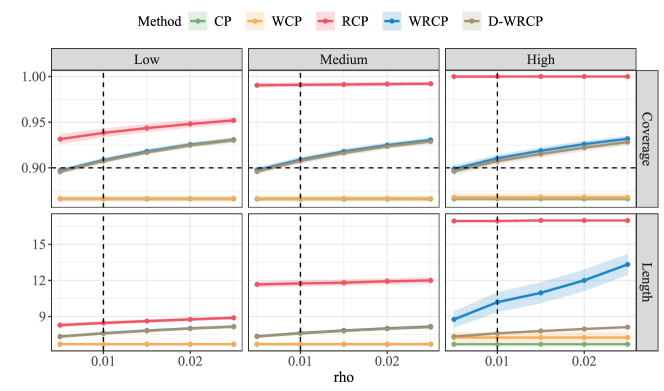
Figure 1: Averaged coverage (top) and prediction interval length (bottom) over $N=100$ independent runs as a function of the robust parameter $\rho$, when the amount of covariate shift is low (left), medium (middle), and high (right). The shaded bars correspond to the $95\%$ confidence intervals. The horizontal dashed line corresponds to the target coverage rate $0.9$, and the vertical dashed line is the true robust parameter $\rho^{*}=0.01$.

6 Real data applications

In this section, we evaluate the performance of all methods on three real datasets: the national study of learning mindsets dataset (Carvalho et al.,, 2019), the ACS income dataset (Ding et al.,, 2021), and the covid information study datasets (Pennycook et al.,, 2020; Roozenbeek et al.,, 2021). For each task, we implement WRCP and D-WRCP, as well as the benchmarks CP, WCP, and RCP with the target coverage level $80\%$. For WRCP and D-WRCP, we choose $f(t)=t\log t$ (the KL-divergence), and consider a sequence of robust parameter $\rho$’s, reporting the averaged coverage rate and prediction set length/cardinality as a function of $\rho$. For RCP, the robust parameter is chosen as $\rho_{\text{RCP}}=\rho+D_{\rm KL}(Q_{X}\,\|\,P_{X})$, where $D_{\rm KL}(Q_{X}\,\|\,P_{X})=\mathbb{E}_{Q_{X}}[\log(\textnormal{d}Q_{X}/\textnormal{d}P_{X})]$ is estimated with Monte Carlo with the set-aside training data.

6.1 National study of learning mindsets

The National Study of Learning Mindsets (NSLM) (Yeager et al.,, 2019; Yeager,, 2019) is a randomized study investigating the effect of instilling students with a growth mindset. Based on the results from NSLM, Carvalho et al., (2019) creates an observational study dataset with similar characteristics to the original study. The observational study dataset contains $10,\!391$ students, where $3,\!384$ received the intervention and $7,\!007$ did not. For each student, the dataset records the treatment status $T$, the outcome $Y$, and ten covariates: S3, C1, C2, C3, XC, X1, X2, X3, X4, X5. We consider the task of predicting $Y(1)$ in the control group, where we wish to construct a prediction interval $\widehat{C}_{f,\rho}(X)$ such that

$$\mathbb{P}\big{(}Y(1)\in\widehat{C}_{f,\rho}(X)\,\big{|}\,T=0\big{)}\geq 80\%.$$

Without observing the counterfactuals, the validity of a procedure cannot be evaluated. As an alternative, we create a semi-synthetic data based on the NSLM dataset. Following the strategy of Carvalho et al., (2019), we generate synthetic potential outcomes from the following model:

$$Y(t)=\mu(x)+\tau(x_{1},x_{2},c_{1})\cdot t+\epsilon,\text{ for }t=0,1.$$

Above, $x$ denotes all the covariates for a student, and $x_{1},x_{2},c_{1}$ corresponds to X1, X2 and C1, respectively. The baseline function $\mu$ is obtained by fitting a generalized additive model (Hastie,, 2017) on the control arm of the original data, and $\epsilon$ is sampled with replacement from the sum of the residual from the fitted model on the original data and a noise term ${\mathcal{N}}(0,0.025)$. The form of the treatment effect is:

$$\tau(x_{1},x_{2},c_{1})=0.228+0.05\cdot\mathds{1}\{x_{1}<0.07\}-0.05\cdot\mathds{1}\{x_{2}<-0.69\}-0.08\cdot\mathds{1}\{c_{1}\in\{1,13,14\}\}.$$

Confounding is introduced by removing two features, X1 and X2.

We consider a sequence of $\rho\in\{0.001,0.005,0.01,0.015,\ldots,0.04\}$. For each run, we randomly select half of the treated units and half of the control units for model fitting; the other half of the treated units are reserved for calibration, while the other half of the control units for evaluation. The nonconformity score function $s(x,y)=|y-\widehat{\mu}(x)|$. Both the regression function $\widehat{\mu}(x)$ and the propensity score function $e(x)$ are fitted with random forest. With each $\rho$, we repeat the above process for $100$ random splits.

Figure 2 plots the resulting coverage rate and prediction interval length as a function of $\rho$. CP and WCP fail to achieve the desired coverage level, while RCP is overly conservative, achieving a much higher coverage rate than the target level. Our methods WRCP and D-WRCP achieve approximate coverage for a wide range of $\rho$, and are much more efficient than RCP.

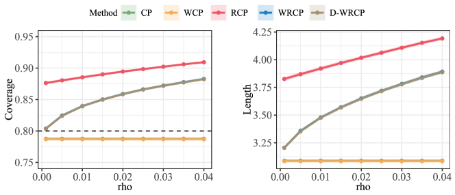
Figure 2: Averaged coverage (left) and prediction interval length (right) over $100$ runs as a function of the robust parameter $\rho$ from experiments on the NSLM dataset. The dashed bar corresponds to the $95\%$ confidence interval and the horizontal dashed line corresponds to the target coverage rate $80\%$.

6.2 ACS income dataset

We further evaluate our procedure for a classification task with the ACS income dataset constructed from the US census data (Ding et al.,, 2021). The target is to predict whether an individual’s annual income is above $50,\!000$ dollars. The specific dataset we use is the version pre-processed by Liu et al., (2023), where we choose the data from New York (NY) as the training set, and that from South Dakota (SD) as the target — as discussed in Liu et al., (2023), both $X$-shift and $Y{\,|\,}X$-shift exist between the training and target population. The training and test set contain $103,\!021$ and $4,\!899$ samples, respectively. For each sample, $9$ features are recorded, where $3$ of them are continuous and $6$ categorical. After introducing the dummy variables, the dimension of $X$ comes to $76$. The response variable $Y=\mathds{1}\{\text{income}\geq 50,\!000\text{ dollars}\}$.

Since $Y$ is binary, we adopt the generalized inverse quantile conformity score introduced by Romano et al., (2020), and the prediction set is a subset of $\{0,1\}$. The weight function $\widehat{w}$ is estimated via XGBoost (Chen and Guestrin,, 2016) with the hyperparameters provided by Liu et al., (2023), and the outcome model $\widehat{\mu}$ is fitted with random forest. The robust parameter $\rho\in\{0.005,0.01,\ldots,0.04\}$. In each run, we randomly select $2000$ samples from the source population, and the same number of samples from the target population. For each $\rho$, we repeat the above process over $100$ random splits and report the averaged coverage and prediction set cardinality.

Figure 3 presents the simulation results of all methods. Ae before, CP and WCP fail to achieve the desired coverage level $80\%$; WCP improves upon CP because it adjusts for the covariate shift. RCP is overly conservative, while our methods again deliver valid and efficient prediction intervals for a wide range of $\rho$’s.

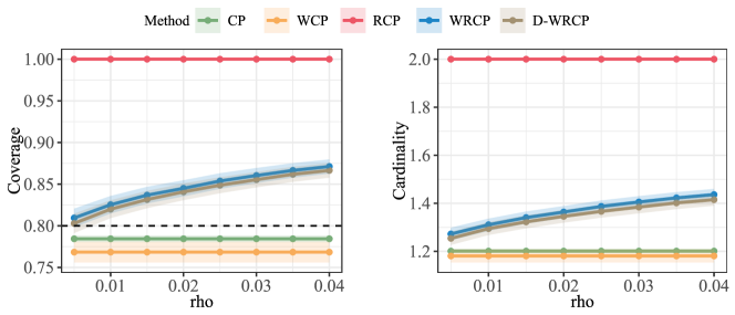
Figure 3: Averaged coverage (left) and prediction set cardinality (right) over $100$ runs as a function of the robust parameter $\rho$ from the experiment on ACS income dataset. The other details are the same as in Figure 2.

6.3 COVID information studies

The covid information studies investigate how a “nudge” for thinking about the accuracy of information can affect the people’s ability to discern fake news when sharing COVID-related headlines. The original study of $856$ participants (Pennycook et al.,, 2020) is first conducted, followed by a replication study (Roozenbeek et al.,, 2021) of $1,\!583$ participants. The original study found a significant interaction term between the intervention and the validity of the headline, while the replication study also found a significant interaction, but with a much smaller magnitude (more details about the comparison between the two studies can be found in Jin et al., 2023a ).

As discussed in Jin et al., 2023a , the discrepancy between the two results can be attributed to the distributional shift in the both the covariates and $Y{\,|\,}X$. Here, instead of estimating the treatment effect, we consider the task of predicting a participant’s rating for willingness to share a headline. Each sample in the dataset corresponds to a participant, where the outcome is the rating for their willingness to share a headline; the predictors include the treatment status (i.e., whether a nugde is sent), the validity of the news, and $10$ other covariates. After removing the samples with missing values, the training and test set consist of $811$ and $1,\!583$ samples, respectively. Each run splits the training and test sets into two halves for model fitting and calibration; The weight function $\widehat{w}$ and the outcome model $\widehat{\mu}$ are both estimated via random forest. The robust parameter $\rho\in\{0.005,0.01,\ldots,0.04\}$, and for each $\rho$ We repeat the above process for $100$ random splits.

Figure 4 demonstrates the results of all methods. For the purpose of visualization, we replace the infinite prediction interval length with $2$ (an upper bound of all the finite realized lengths) when plotting the averaged prediction interval length. In this example, we again see that CP and WCP fail to achieve the desired coverage level, with WCP being slightly better than CP due to the adjustment for covariate shift. The proposed methods WRCP and D-WRCP achieve approximate coverage for a wide range of $\rho$’s, and are much more efficient than RCP.

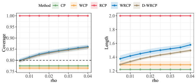
Figure 4: Averaged coverage (left) and prediction interval length (right) over $100$ runs as a function of the robust parameter $\rho$ from the experiment on covid study datasets. The other details are the same as in Figure 2.

7 Discussion

In this paper, we provide a fine-grained approach to quantifying the uncertainty of predictive models by distinguishing sources of distributional shift and providing different treatments. We propose two new methods, WRCP and its debiased version D-WRCP, that achieve validity and efficiency under a wide range of distributional shifts, as demonstrated in the simulation and real data experiments. This paper opens up several interesting directions for future work. First, it would be interesting to investigate methods for identifying (an upper bound) of the robust parameter $\rho$ when we have a small amount of supervised data from the target population. Second, can we extend this fine-grained approach to other distributional shift models and improves the efficiency of the corresponding methodologies? Last but not least, there can be other ways to decompose the distributional shifts — it remains to be understood the optimal decomposition in different settings and the corresponding treatments.

Reproducibility

All the numerical results in this paper can be reproduced with the code available at https://github.com/zhimeir/finegrained-conformal-paper.

Acknowledgements

The authors would like to thank Wharton High Performance Computing for the computational resources and the support from the staff members. The authors would also like to thank Ying Jin for the feedback on the manuscript.

Appendix A Auxiliary lemmas

Lemma 1 (Data processing inequality (Cover,, 1999)).

Let $X,Y,Z$ denote random variables drawn from a Markov chain in the order (denoted by $X\rightarrow Y\rightarrow Z$) that the conditional distribution of $Z$ depends only on $Y$ and is conditionally independent of $X$. Then if $X\rightarrow Y\rightarrow Z$, we have $I(X;Y)\geq I(X;Z)$, where $I(X;Y)$ is the mutual information between $X$ and $Y$.

Lemma 2 (Adapted from Lemma A.1 of Cauchois et al., (2023)).

Let $f:\mathbb{R}\mapsto\mathbb{R}$ be a closed convex function such that $f(1)=0$ and $f(t)<\infty$ for all $t>0$. The function $g_{f,\rho}(\beta)$ has the following properties.

• $(\rho,\beta)\rightarrow g_{f,\rho}(\beta)$ is a convex function and continuous in $\beta\in[0,1]$ and $\rho\in(0,\infty)$.

• $g_{f,\rho}(\beta)$ is non-increasing in $\rho$ and non-decreasing in $\beta$. Moreover, for all $\rho>0$, there exists $\beta_{0}(\rho)\,:=\,\sup\big{\{}\beta\in(0,1){\,|\,}g_{f,\rho}(\beta)=0\big{\}}$, and $g_{f,\rho}(\beta)$ is strictly increasing for $\beta>\beta_{0}(\rho)$.

Appendix B Technical Proofs

B.1 Proof of Theorem 1

For notional simplicity, let $A\,:=\,\big{\{}Y_{n+1}\in\widehat{C}_{f,\rho}(X_{n+1})\big{\}}$. We aim to show that

$$\mathbb{P}_{(X_{n+1},Y_{n+1})\sim Q_{X,Y}}(A)\geq 1-\alpha.$$

Denote by $\text{Bern}(p)$ the Bernoulli distribution with success probability $p$. By data processing inequality (Lemma 1), we have that

$$D_{f}\big{(}Q_{Y{\,|\,}X}\,\|\,P_{Y{\,|\,}X}\big{)}\geq D_{f}\big{(}\text{Bern}\big{(}\mathbb{P}_{Y_{n+1}\sim Q_{Y{\,|\,}X}}(A{\,|\,}X_{n+1},{\mathcal{D}})\big{)}\,\big{\|}\,\text{Bern}\big{(}\mathbb{P}_{Y_{n+1}\sim P_{Y{\,|\,}X}}(A{\,|\,}X_{n+1},{\mathcal{D}})\big{)}\big{)}.$$ (13)

Recall that $Q\in{\mathcal{P}}(\rho;P)$. We then have

$$\rho \geq D_{f}\big{(}Q_{Y{\,|\,}X}\,\|\,P_{Y{\,|\,}X}\big{)}$$ (14)

$$\geq D_{f}\big{(}\text{Bern}\big{(}\mathbb{P}_{Y_{n+1}\sim Q_{Y{\,|\,}X}}(A{\,|\,}X_{n+1},{\mathcal{D}})\big{)}\,\big{\|}\,\text{Bern}\big{(}\mathbb{P}_{Y_{n+1}\sim P_{Y{\,|\,}X}}(A{\,|\,}X_{n+1},{\mathcal{D}})\big{)}\big{)}$$ (15)

$$=\mathbb{P}_{Y_{n+1}\sim P_{Y{\,|\,}X}}(A{\,|\,}X_{n+1},{\mathcal{D}})\cdot f\bigg{(}\frac{\mathbb{P}_{Y_{n+1}\sim Q_{Y{\,|\,}X}}(A{\,|\,}X_{n+1},{\mathcal{D}})}{\mathbb{P}_{Y_{n+1}\sim P_{Y{\,|\,}X}}(A{\,|\,}X_{n+1},{\mathcal{D}})}\bigg{)}$$ (16)

$$\qquad\qquad\qquad\qquad\qquad+\big{(}1-\mathbb{P}_{Y\sim P_{Y{\,|\,}X}}(A{\,|\,}X_{n+1},{\mathcal{D}})\big{)}\cdot f\bigg{(}\frac{1-\mathbb{P}_{Y\sim Q_{Y{\,|\,}X}}(A{\,|\,}X_{n+1},{\mathcal{D}})}{1-\mathbb{P}_{Y\sim P_{Y{\,|\,}X}}(A{\,|\,}X_{n+1},{\mathcal{D}})}\bigg{)},$$ (17)

where the last step follows from the definition of the $f$-divergence. Combining the above and the definition of $g_{f,\rho}$, one can obtain that almost surely

$$g_{f,\rho}\big{(}\mathbb{P}_{Y\sim P_{Y{\,|\,}X}}(A)\big{)}\leq\mathbb{P}_{Y\sim Q_{Y{\,|\,}X}}(A).$$ (18)

Next, we take the expectation over the randomness of the training set ${\mathcal{D}}$ and $X_{n+1}$

$$\mathbb{P}_{{\mathcal{D}},\,(X_{n+1},Y_{n+1})\sim Q_{X,Y}}(A) =\mathbb{E}_{{\mathcal{D}},\,X_{n+1}\sim Q_{X}}\big{[}\mathbb{P}_{Y_{n+1}\sim Q_{Y{\,|\,}X}}\big{(}A{\,|\,}X_{n+1},{\mathcal{D}}\big{)}\big{]}$$

$$\geq\mathbb{E}_{{\mathcal{D}},X_{n+1}\sim Q_{X}}\Big{[}g_{f,\rho}\big{(}\mathbb{P}_{Y\sim P_{Y{\,|\,}X}}(A{\,|\,}X_{n+1},{\mathcal{D}})\big{)}\Big{]},$$ (19)

where the last inequality is because of (18). Since $g_{f,\rho}$ is convex (Lemma 2), Jensen’s inequality implies

$$\mathbb{E}_{{\mathcal{D}},X_{n+1}\sim Q_{X}}\Big{[}g_{f,\rho}\big{(}\mathbb{P}_{Y\sim P_{Y{\,|\,}X}}(A{\,|\,}X_{n+1},{\mathcal{D}})\big{)}\Big{]} \geq g_{f,\rho}\Big{(}\mathbb{P}_{{\mathcal{D}},(X_{n+1},Y_{n+1})\sim Q_{X}\times P_{Y{\,|\,}X}}(A)\Big{)}.$$ (20)

By Tibshirani et al., (2019, Corollary 1) and the construction of $\widehat{C}_{f,\rho}(X_{n+1})$, there is

$$\mathbb{P}_{{\mathcal{D}},(X_{n+1},Y_{n+1})\sim Q_{X}\times P_{Y{\,|\,}X}}(A)\geq g_{f,\rho}^{-1}\big{(}1-\alpha\big{)}.$$ (21)

Again leveraging the monotonicity of $g_{f,\rho}(\beta)$ in $\beta$, we arrive at

$$\mathbb{P}_{{\mathcal{D}},(X_{n+1},Y_{n+1})\sim Q_{X,Y}}(A) \geq g_{f,\rho}\big{(}g_{f,\rho}^{-1}(1-\alpha)\big{)}.$$ (22)

When $g_{f,\rho}(1)\geq 1-\alpha$, we prove that $g_{f,\rho}\big{(}g^{-1}_{f,\rho}(1-\alpha)\big{)}\geq 1-\alpha$ by contradiction. Suppose otherwise that $g_{f,\rho}\big{(}g^{-1}_{f,\rho}(1-\alpha)\big{)}<1-\alpha$. Then $g^{-1}_{f,\rho}(1-\alpha)<1$. By the continuity of $g_{f,\rho}(\beta)$ in $\beta$, there exists a small $\varepsilon>0$, such that $g_{f,\rho}(\beta)<1-\alpha$ for all $\beta\in[g^{-1}_{f,\rho}(1-\alpha),g^{-1}_{f,\rho}(1-\alpha)+\epsilon]$, which contradicts the definition of $g^{-1}_{f,\rho}(1-\alpha)$. The proof is therefore completed.

B.2 Proof of Theorem 2

Throughout the proof, we condition on ${\mathcal{D}}_{\textnormal{tr}}^{(0)}\cup{\mathcal{D}}_{\textnormal{test}}^{(1-k)}$, and for notational simplicity we do not explicitly write the conditional probability and expectation when the context is clear.

We start by defining a new distribution $\widetilde{Q}_{X,Y}=\widetilde{Q}_{X}\times P_{Y{\,|\,}X}$ such that

$$\frac{d\tilde{Q}_{X}}{dP_{X}}(x)=\frac{\widehat{w}^{(k)}(x)}{\mathbb{E}_{X\sim P_{X}}[\widehat{w}^{(k)}(X)]}.$$

Let $A=\big{\{}Y_{n+j}\in\widehat{C}_{f,\rho,j}(X_{n+j})\big{\}}$. If $(X_{n+j},Y_{n+j})$ were indeed sampled from $\widetilde{Q}_{X,Y}$, then by Lemma 1 of Tibshirani et al., (2019), we have

$$\mathbb{P}_{{\mathcal{D}}_{\textnormal{tr}}^{(1)},(X_{n+j},Y_{n+j})\sim\widetilde{Q}_{X,Y}}(A)\geq g_{f,\rho}^{-1}(1-\alpha).$$ (23)

Meanwhile, by the definition of the TV distance,

$$\Big{|}\mathbb{P}_{(X_{n+j},Y_{n+j})\sim\widetilde{Q}_{X}\times P_{Y{\,|\,}X}}\big{(}A{\,|\,}{\mathcal{D}}_{\textnormal{tr}}^{(1)}\big{)}-\mathbb{P}_{(X_{n+j},Y_{n+j})\sim Q_{X}\times P_{Y{\,|\,}X}}\big{(}A{\,|\,}{\mathcal{D}}_{\textnormal{tr}}^{(1)}\big{)}\Big{|}$$ (24)

$$\leq\leavevmode\nobreak\ D_{\text{TV}}\big{(}\widetilde{Q}_{X}\times Q_{Y{\,|\,}X}\,\|\,Q_{X}\times Q_{Y{\,|\,}X}\big{)}$$ (25)

$$=\leavevmode\nobreak\ D_{\text{TV}}(\widetilde{Q}_{X}\,\|\,Q_{X})=\frac{1}{2}\mathbb{E}_{X\sim P_{X}}\bigg{[}\Big{|}\frac{\widehat{w}^{(k)}(X)}{\mathbb{E}_{X\sim P_{X}}[\widehat{w}^{(k)}(X)]}-w(X)\Big{|}\bigg{]}.$$ (26)

The above inequality implies that

$$\mathbb{P}_{(X_{n+j},Y_{n+j})\sim Q_{X}\times P_{Y{\,|\,}X}}\big{(}A\,\big{|}\,{\mathcal{D}}_{\textnormal{tr}}^{(1)}\big{)}\geq\mathbb{P}_{(X_{n+j},Y_{n+j})\sim\widetilde{Q}_{X}\times P_{Y{\,|\,}X}}\big{(}A\,\big{|}\,{\mathcal{D}}_{\textnormal{tr}}^{(1)}\big{)}-\frac{1}{2}\mathbb{E}_{X\sim P_{X}}\bigg{[}\Big{|}\frac{\widehat{w}^{(k)}(X)}{\mathbb{E}_{X\sim P_{X}}[\widehat{w}^{(k)}(X)]}-w(X)\Big{|}\bigg{]}.$$ (27)

Taking expectation over ${\mathcal{D}}_{\textnormal{tr}}^{(1)}$, we have

$$\mathbb{P}_{{\mathcal{D}}_{\textnormal{tr}}^{(1)},(X_{n+j},Y_{n+j})\sim{Q}_{X}\times P_{Y{\,|\,}X}}(A)$$ (28)

$$\geq\leavevmode\nobreak\ \mathbb{P}_{{\mathcal{D}}_{\textnormal{tr}}^{(1)},(X_{n+j},Y_{n+j})\sim\widetilde{Q}_{X,Y}}(A)-\frac{1}{2}\mathbb{E}_{X\sim P_{X}}\bigg{[}\Big{|}\frac{\widehat{w}^{(k)}(X)}{\mathbb{E}_{X\sim P_{X}}[\widehat{w}^{(k)}(X)]}-w(X)\Big{|}\bigg{]}$$ (29)

$$\geq\leavevmode\nobreak\ g_{f,\rho}^{-1}(1-\alpha)-\frac{1}{2}\mathbb{E}_{X\sim P_{X}}\bigg{[}\Big{|}\frac{\widehat{w}^{(k)}(X)}{\mathbb{E}_{X\sim P_{X}}[\widehat{w}^{(k)}(X)]}-w(X)\Big{|}\bigg{]},$$ (30)

where the last step follows from (23). Following the same argument as in the proof of Theorem 1 (Eqn. (B.1) and (20)), we have

$$\mathbb{P}_{{\mathcal{D}}_{\textnormal{tr}}^{(1)},(X_{n+1},Y_{n+1})\sim Q_{X,Y}}(A)$$

$$\geq\leavevmode\nobreak\ g_{f,\rho}\Big{(}\mathbb{P}_{{\mathcal{D}}_{\textnormal{tr}}^{(1)},(X_{n+j},Y_{n+j})\sim Q_{X}\times P_{Y{\,|\,}X}}(A)\Big{)}$$

$$\geq\leavevmode\nobreak\ g_{f,\rho}\Bigg{(}g_{f,\rho}^{-1}(1-\alpha)-\frac{1}{2}\mathbb{E}_{X\sim P_{X}}\bigg{[}\Big{|}\frac{\widehat{w}^{(k)}(X)}{\mathbb{E}_{X\sim P_{X}}[\widehat{w}^{(k)}(X)]}-w(X)\Big{|}\bigg{]}\Bigg{)},$$ (31)

where the last inequality is because $g_{f,\rho}(\beta)$ is non-decreasing in $\beta$. Since $g_{f,\rho}(\beta)$ is convex in $(0,1)$, the left derivative exists and by the separating hyperplane theorem, we further have

$$\eqref{eq:first_result}\geq g_{f,\rho}\big{(}g^{-1}_{f,\rho}(1-\alpha)\big{)}-\frac{1}{2}g^{\prime}_{f,\rho}\big{(}g^{-1}_{f,\rho}(1-\alpha)\big{)}\cdot\mathbb{E}_{X\sim P_{X}}\bigg{[}\Big{|}\frac{\widehat{w}^{(k)}(X)}{\mathbb{E}_{X\sim P_{X}}[\widehat{w}^{(k)}(X)]}-w(X)\Big{|}\bigg{]}.$$

As shown in the proof of Theorem 1, when $g_{f,\rho}(1)\geq 1-\alpha$, $g_{f,\rho}\big{(}g_{f,\rho}^{-1}(1-\alpha)\big{)}\geq 1-\alpha$, and we conclude the proof.

B.3 Proof for the doubly robust prediction intervals

We start by proving that the $D_{f,\rho,n+j}^{\text{DR}}(X_{n+j})$ is training-conditionally valid in Theorem 5, and then show that Theorem 3 is a direct consequence of Theorem 5.

Theorem 5.

For any $k\in\{0,1\}$, assume that

1. $\widehat{w}^{(k)}(x)\leq w_{\max}\cdot\mathbb{E}_{P_{X}}[\widehat{w}^{(k)}(X)]$;

2. $\widehat{m}^{(k)}(x;t)\in[0,1]$ is non-decreasing and right-continuous in $t$.

Denote the product estimation error by

$$\textnormal{EstErr}^{(k)}(t)=\big{\|}\mathds{1}\{s(X,Y;\widehat{\mu}^{(k)})\leq t\}-\widehat{m}^{(k)}(X;t)\big{\|}_{L_{2}(P)}\bigg{\|}\frac{\widehat{w}^{(k)}(X)}{\mathbb{E}_{X\sim P_{X}}[\widehat{w}^{(k)}(X)]}-w(X)\bigg{\|}_{L_{2}(P)},$$

where $\|\cdot\|_{L_{2}(P)}$ denotes the $L_{2}$-norm under $P$, and the expectation is taken conditional on ${\mathcal{D}}_{\textnormal{tr}}^{(1-k)}$ and ${\mathcal{D}}_{\textnormal{test}}^{(1-k)}$. Then for any $\delta>0$ and any unit $n+j\in{\mathcal{I}}_{\textnormal{test}}^{(k)}$, with probability at least $1-\delta$,

$$\mathbb{P}_{(X_{n+j},Y_{n+j})\sim Q_{X,Y}}\big{(}Y_{n+j}\in\widehat{C}_{f,\rho,n+j}^{\textnormal{DR}}(X_{n+j})\,\big{|}\,{\mathcal{D}}_{\textnormal{tr}}^{(k)},{\mathcal{D}}_{\textnormal{test},j}^{(k)},{\mathcal{D}}_{\textnormal{tr}}^{(1-k)},{\mathcal{D}}_{\textnormal{test}}^{(1-k)}\big{)}$$

$$\geq\leavevmode\nobreak\ g_{f,\rho}\big{(}g^{-1}_{f,\rho}(1-\alpha)\big{)}-g^{\prime}_{f,\rho}\big{(}g^{-1}(1-\alpha)\big{)}\times\Bigg{\{}\sup_{t\in{\mathcal{T}}(\alpha)}\textnormal{EstErr}^{(k)}(t)+\sqrt{\log\Big{(}\frac{1}{\delta}\Big{)}\cdot\bigg{(}\frac{9w_{\max}^{2}}{|{\mathcal{I}}_{\textnormal{tr}}^{(k)}|}+\frac{1}{|{\mathcal{I}}_{\textnormal{test},j}^{(k)}|}\bigg{)}}\Bigg{\}},$$

where $g^{\prime}_{f,\rho}$ is the left derivative of $g_{f,\rho}$. If $g_{f,\rho}(1)\geq 1-\alpha$, then with probability at least $1-\delta$,

$$\mathbb{P}_{(X_{n+j},Y_{n+j})\sim Q_{X,Y}}\big{(}Y_{n+j}\in\widehat{C}_{f,\rho,n+j}^{\textnormal{DR}}(X_{n+j})\,\big{|}\,{\mathcal{D}}_{\textnormal{tr}}^{(k)},{\mathcal{D}}_{\textnormal{test},j}^{(k)},{\mathcal{D}}_{\textnormal{tr}}^{(1-k)},{\mathcal{D}}_{\textnormal{test}}^{(1-k)}\big{)}$$

$$\geq\leavevmode\nobreak\ 1-\alpha-g^{\prime}_{f,\rho}\big{(}g^{-1}(1-\alpha)\big{)}\times\Bigg{\{}\sup_{t\in{\mathcal{T}}(\alpha)}\textnormal{EstErr}^{(k)}(t)+\sqrt{\log\bigg{(}\frac{1}{\delta}\Big{)}\cdot\Big{(}\frac{9w_{\max}^{2}}{|{\mathcal{I}}_{\textnormal{tr}}^{(k)}|}+\frac{1}{|{\mathcal{I}}_{\textnormal{test},j}^{(k)}|}\bigg{)}}\Bigg{\}}.$$

Proof.

Without loss of generality, assume $k=1$. Throughout, we condition on ${\mathcal{D}}_{\textnormal{tr}}^{(0)}\cup{\mathcal{D}}_{\textnormal{test}}^{(0)}$ without explicitly writing the conditioning event when the context is clear. For notational simplicity, we define the normalized weight as

$$\widetilde{w}^{(k)}(x)=\frac{\widehat{w}^{(k)}(x)}{\mathbb{E}_{X\sim P_{X}}[\widehat{w}^{(k)}(X)]}.$$

In the proof we leave out the dependence on $k$, writing $\widehat{m}(X;t)$ and $\widetilde{w}(X)$ in place of $\widehat{m}^{(1)}(X;t)$ and $\widetilde{w}^{(1)}(X)$; additionally, we refer to $\mathbb{E}_{(X,Y)\sim P_{X,Y}}$ as $\mathbb{E}_{P_{X,Y}}$, with the same rule applied to the expectation/probability under other distributions, and let $n_{\textnormal{tr}}=|{\mathcal{I}}_{\textnormal{tr}}^{(1)}|$ and $n_{\textnormal{test}}=|{\mathcal{I}}_{\textnormal{test},j}^{(1)}|$.

For any $t\in\mathbb{R}$, we define the oracle CDF $F(t)=\mathbb{P}_{Q_{X}\times P_{Y{\,|\,}X}}\big{(}s(X,Y)\leq t\big{)}$, and for any $\xi\in[0,g^{-1}_{f,\rho}(1-\alpha)]$, the perturbed oracle quantile $q^{*}(\xi)$ can be equivalently written as

$$q^{*}(\xi)=\inf\big{\{}t\in\mathbb{R}:F(t)\geq g^{-1}_{f,\rho}(1-\alpha)-\xi\big{\}}.$$

Consider the error of margin

$$\Delta=\sup_{\kappa\cdot q^{*}(\bar{\Delta})\leq t\leq q^{*}(0)}\textnormal{EstErr}(t)+\sqrt{\log\Big{(}\frac{1}{\delta}\Big{)}\cdot\Big{(}\frac{9w_{\max}^{2}}{n_{\textnormal{tr}}}+\frac{1}{n_{\textnormal{test}}}\Big{)}},$$

where $\kappa\in(0,1)$ is a constant that can be arbitrarily close to $1$ and

$$\bar{\Delta}=\Bigg{\{}\sup_{0\leq t\leq q^{*}(0)}\textnormal{EstErr}(t)+\sqrt{\log\Big{(}\frac{1}{\delta}\Big{)}\cdot\Big{(}\frac{9w_{\max}^{2}}{n_{\textnormal{tr}}}+\frac{1}{n_{\textnormal{test}}}\Big{)}}\Bigg{\}}\wedge g^{-1}_{f,\rho}(1-\alpha).$$

Here, $a\wedge b=\min(a,b)$ and $\Delta$ is fully deterministic conditional on ${\mathcal{D}}_{\textnormal{tr}}^{(0)}\cup{\mathcal{D}}_{\textnormal{test}}^{(0)}$.

The proof consists of two steps: (1) we show that, with high probability, $\widehat{q}\geq q^{*}(\Delta)$. and therefore $\widehat{q}$ is no less than the $(g^{-1}_{f,\rho}(1-\alpha)-\Delta)$-th quantile under $Q_{X}\times P_{Y{\,|\,}X}$, and (2) $\widehat{q}$ is approximately an upper bound of the $(1-\alpha)$-th quantile under $Q_{X,Y}$.

Step (1).

On the event $\{q^{*}(\Delta)\leq\widehat{q}\}$,

$$\mathbb{P}\big{(}s(X_{n+j},Y_{n+j})\leq\widehat{q}{\,|\,}{\mathcal{D}}_{\textnormal{tr}}^{(1)},{\mathcal{D}}_{\textnormal{test},j}^{(1)}\big{)}=F(\widehat{q})\stackrel{{\scriptstyle\text{(i)}}}{{\geq}}F(q^{*}(\Delta))\stackrel{{\scriptstyle\text{(ii)}}}{{\geq}}g^{-1}_{f,\rho}(1-\alpha)-\Delta,$$

where step (i) follows from the monotonicity of $F(t)$, and step (ii) is by the definition of $q^{*}(\Delta)$ and that $F(t)$ is right-continuous. It then suffices to control the probability of $\{q^{*}(\Delta)>\widehat{q}\}$. Fixing $\delta\in[0,1]$, we aim at showing that

$$\mathbb{P}\big{(}\widehat{q}<q^{*}(\Delta)\big{)}\leq\delta.$$

The above is trivial when $\Delta\geq g^{-1}_{f,\rho}(1-\alpha)$. We proceed assuming that $\Delta<g^{-1}_{f,\rho}(1-\alpha)$.

For any $\varepsilon>0$, we have that $F(q^{*}(\Delta)-\varepsilon)<g^{-1}_{f,\rho}(1-\alpha)-\Delta$ by the definition of $q^{*}(\Delta)$. If $\widehat{q}\leq q^{*}(\Delta)-\varepsilon$, then the choice of $\widehat{q}$ implies that

$$\widehat{p}(q^{*}(\Delta)-\varepsilon)\geq g^{-1}_{f,\rho}(1-\alpha).$$

In other words,

$$\mathbb{P}\big{(}\widehat{q}\leq q^{*}(\Delta)-\varepsilon\big{)}\leq\leavevmode\nobreak\ \mathbb{P}\Big{(}\widehat{p}(q^{*}(\Delta)-\varepsilon)\geq g^{-1}_{f,\rho}(1-\alpha)\Big{)}.$$ (32)

For better readability, we use $\bar{t}$ to represent $q^{*}(\Delta)-\varepsilon$, and let $Z_{i}=\mathds{1}\{S_{i}\leq{\bar{t}}\}-\widehat{m}(X_{i};{\bar{t}})$ in the following. The right-hand side of (32) can be further upper bounded as

$$\mathbb{P}\big{(}\widehat{p}({\bar{t}})\geq g^{-1}_{f,\rho}(1-\alpha)\big{)}$$

$$=\leavevmode\nobreak\ \mathbb{P}\bigg{(}\sum_{i\in{\mathcal{I}}_{\textnormal{tr}}^{(1)}}\widetilde{w}(X_{i})Z_{i}+\Big{(}\sum_{i\in{\mathcal{I}}_{\textnormal{tr}}^{(1)}}\widetilde{w}(X_{i})\Big{)}\Big{(}\frac{1}{n_{\textnormal{test}}}\sum_{i\in{\mathcal{I}}_{\textnormal{test},j}^{(1)}}\widehat{m}(X_{i};{\bar{t}})-g_{f,\rho}^{-1}(1-\alpha)\Big{)}\geq 0\bigg{)}$$

$$\leq\leavevmode\nobreak\ \mathbb{E}\Bigg{[}\exp\bigg{\{}\eta\bigg{(}\sum_{i\in{\mathcal{I}}_{\textnormal{tr}}^{(1)}}\widetilde{w}(X_{i})Z_{i}+\Big{(}\sum_{i\in{\mathcal{I}}_{\textnormal{tr}}^{(1)}}\widetilde{w}(X_{i})\Big{)}\Big{(}\frac{1}{n_{\textnormal{test}}}\sum_{i\in{\mathcal{I}}_{\textnormal{test},j}^{(1)}}\widehat{m}(X_{i};{\bar{t}})-g_{f,\rho}^{-1}(1-\alpha)\Big{)}\bigg{)}\bigg{\}}\Bigg{]},$$ (33)

where $\eta>0$ is some constant to be determined and the last step follows from Markov’s inequality.

Conditional on $\{X_{i}\}_{i\in{\mathcal{I}}_{\textnormal{tr}}^{(1)}}$, $Z_{i}-\mathbb{E}[Z_{i}{\,|\,}X_{i}]$ are $\frac{1}{4}$-subgaussian random variables. Therefore,

$$\mathbb{E}\bigg{[}\exp\Big{\{}\eta\Big{(}\sum_{i\in{\mathcal{I}}_{\textnormal{tr}}^{(1)}}\widetilde{w}(X_{i})\cdot\big{(}Z_{i}-\mathbb{E}[Z_{i}{\,|\,}X_{i}]\big{)}\Big{)}\Big{\}}\,\Big{|}\,\{X_{i}\}_{i\in{\mathcal{I}}_{\textnormal{tr}}^{(1)}}\bigg{]}\leq\exp\Big{(}\frac{\eta^{2}w_{\max}^{2}n_{\textnormal{tr}}}{8}\Big{)}.$$

The above implies that

$$\eqref{eq:dr_step1}\leq\leavevmode\nobreak\ \exp\Big{(}\frac{\eta^{2}w_{\max}^{2}n_{\textnormal{tr}}}{8}\Big{)}\cdot\mathbb{E}\Bigg{[}\exp\Bigg{\{}\eta\bigg{(}\sum_{i\in{\mathcal{I}}_{\textnormal{tr}}^{(1)}}\widetilde{w}(X_{i})\mathbb{E}[Z_{i}{\,|\,}X_{i}]$$

$$\qquad\qquad\qquad\qquad\qquad\qquad+\Big{(}\sum_{i\in{\mathcal{I}}_{\textnormal{tr}}^{(1)}}\widetilde{w}(X_{i})\Big{)}\Big{(}\frac{1}{n_{\textnormal{test}}}\sum_{i\in{\mathcal{I}}_{\textnormal{test},j}}\widehat{m}(X_{i};{\bar{t}})-g_{f,\rho}^{-1}(1-\alpha)\Big{)}\bigg{)}\Bigg{\}}\Bigg{]}$$

$$\leq\leavevmode\nobreak\ \exp\Big{(}\frac{\eta^{2}w_{\max}^{2}n_{\textnormal{tr}}}{8}\Big{)}\cdot\mathbb{E}\Bigg{[}\exp\Bigg{\{}2\eta\bigg{(}\sum_{i\in{\mathcal{I}}_{\textnormal{tr}}^{(1)}}\Big{(}\widetilde{w}(X_{i})\mathbb{E}[Z_{i}{\,|\,}X_{i}]+\frac{1}{n_{\textnormal{test}}}\sum_{\ell\in{\mathcal{I}}_{\textnormal{test},j}^{(1)}}\widehat{m}(X_{\ell};{\bar{t}})-g_{f,\rho}^{-1}(1-\alpha)\Big{)}\bigg{)}\Bigg{\}}\Bigg{]}^{1/2}$$

$$\qquad\qquad\times\mathbb{E}\Bigg{[}\exp\bigg{(}2\eta\sum_{i\in{\mathcal{I}}_{\textnormal{tr}}^{(1)}}\big{(}\widetilde{w}(X_{i})-1\big{)}\cdot\Big{(}\frac{1}{n_{\textnormal{test}}}\sum_{\ell\in{\mathcal{I}}_{\textnormal{test},j}^{(1)}}\widehat{m}(X_{\ell};{\bar{t}})-g_{f,\rho}^{-1}(1-\alpha)\Big{)}\bigg{)}\Bigg{]}^{1/2},$$

where the last inequality follows from the Cauchy-Schwarz inequality. Since ${\mathcal{D}}_{\textnormal{test}}^{(1)}$ is independent of ${\mathcal{D}}_{\textnormal{tr}}^{(1)}$, conditional on ${\mathcal{D}}_{\textnormal{test}}^{(1)}$, there is

$$\mathbb{E}\Bigg{[}\exp\bigg{(}2\eta\sum_{i\in{\mathcal{I}}_{\textnormal{tr}}^{(1)}}\big{(}\widetilde{w}(X_{i})-1\big{)}\Big{(}\frac{1}{n_{\textnormal{test}}}\sum_{\ell\in{\mathcal{I}}_{\textnormal{test},j}^{(1)}}\widehat{m}(X_{\ell};{\bar{t}})-g_{f,\rho}^{-1}(1-\alpha)\Big{)}\bigg{)}\,\bigg{|}\,{\mathcal{D}}_{\textnormal{test}}^{(1)}\Bigg{]}^{1/2}\leq\exp\big{(}\eta^{2}w_{\max}^{2}n_{\textnormal{tr}}\big{)},$$

where we use the sub-gaussianity of $\widetilde{w}(X_{i})$. Recalling that $F({\bar{t}})<g^{-1}_{f,\rho}(1-\alpha)-\Delta$, we have that

$$\mathbb{E}\Bigg{[}\exp\Bigg{\{}2\eta\bigg{(}\sum_{i\in{\mathcal{I}}_{\textnormal{tr}}^{(1)}}\Big{(}\widetilde{w}(X_{i})\mathbb{E}[Z_{i}{\,|\,}X_{i}]+\frac{1}{n_{\textnormal{test}}}\sum_{\ell\in{\mathcal{I}}_{\textnormal{test},j}^{(1)}}\widehat{m}(X_{\ell};{\bar{t}})-g_{f,\rho}^{-1}(1-\alpha)\Big{)}\bigg{)}\Bigg{\}}\Bigg{]}^{1/2}$$

$$\leq\leavevmode\nobreak\ \mathbb{E}\Bigg{[}\exp\Bigg{\{}2\eta\bigg{(}\sum_{i\in{\mathcal{I}}_{\textnormal{tr}}^{(1)}}\Big{(}\widetilde{w}(X_{i})\mathbb{E}[Z_{i}{\,|\,}X_{i}]+\frac{1}{n_{\textnormal{test}}}\sum_{\ell\in{\mathcal{I}}_{\textnormal{test},j}^{(1)}}\widehat{m}(X_{\ell};{\bar{t}})-F({\bar{t}})-\Delta\Big{)}\bigg{)}\Bigg{\}}\Bigg{]}^{1/2}.$$ (34)

By definition, $F({\bar{t}})=\mathbb{P}_{Q_{X}\times P_{Y{\,|\,}X}}(s(X,Y)\leq{\bar{t}})=\mathbb{E}_{P_{X,Y}}[w(X)Z]+\mathbb{E}_{Q_{X}}[\widehat{m}(X;{\bar{t}})]$. Therefore,

$$\big{|}F({\bar{t}})-\mathbb{E}_{P_{X,Y}}[\widetilde{w}(X)Z]-\mathbb{E}_{Q_{X}}[\widehat{m}(X;{\bar{t}})]\big{|}$$

$$\leq\leavevmode\nobreak\ \bigg{|}\mathbb{E}_{P_{X,Y}}\Big{[}\big{(}w(X)-\widetilde{w}(X)\big{)}\cdot\big{(}\mathds{1}\{s(X,Y)\leq{\bar{t}}\}-\widehat{m}(X;{\bar{t}})\big{)}\Big{]}\bigg{|}$$

$$\leq\leavevmode\nobreak\ \big{\|}w(X)-\widetilde{w}(X)\big{\|}_{L_{2}(P)}\cdot\big{\|}\mathds{1}\{s(X,Y)\leq{\bar{t}}\}-\widehat{m}(X;{\bar{t}})\big{\|}_{L_{2}(P)}$$

$$=\leavevmode\nobreak\ \textnormal{EstErr}({\bar{t}}).$$ (35)

The last inequality follows from the Cauchy-Schwarz inequality.

Next, we focus on the following quantity:

$$\mathbb{E}\Bigg{[}\exp\bigg{\{}2\eta\bigg{(}\sum_{i\in{\mathcal{I}}_{\textnormal{tr}}^{(1)}}\Big{(}\widetilde{w}(X_{i})\mathbb{E}[Z_{i}{\,|\,}X_{i}]-\mathbb{E}_{P_{X,Y}}[\widetilde{w}(X)Z]\Big{)}+\frac{n_{\textnormal{tr}}}{n_{\textnormal{test}}}\sum_{i\in{\mathcal{I}}_{\textnormal{test},j}^{(1)}}\big{(}\widehat{m}(X_{i};{\bar{t}})-\mathbb{E}_{Q_{X}}[\widehat{m}(X;{\bar{t}})]\big{)}\Big{)}\bigg{)}\bigg{\}}\Bigg{]}$$

$$=\leavevmode\nobreak\ \mathbb{E}\Bigg{[}\exp\bigg{\{}2\eta\sum_{i\in{\mathcal{I}}_{\textnormal{tr}}^{(1)}}\Big{(}\widetilde{w}(X_{i})\mathbb{E}[Z_{i}{\,|\,}X_{i}]-\mathbb{E}_{P_{X,Y}}[\widetilde{w}(X)Z]\Big{)}\bigg{\}}\Bigg{]}$$

$$\qquad\qquad\qquad\qquad+\mathbb{E}\Bigg{[}\exp\bigg{\{}\frac{2\eta\cdot n_{\textnormal{tr}}}{n_{\textnormal{test}}}\sum_{i\in{\mathcal{I}}_{\textnormal{test},j}^{(1)}}\Big{(}\widehat{m}(X_{i};{\bar{t}})-\mathbb{E}_{Q_{X}}[\widehat{m}(X;{\bar{t}})]\Big{)}\bigg{\}}\Bigg{]}$$

$$\leq\leavevmode\nobreak\ \exp\Big{(}2\eta^{2}w_{\max}^{2}n_{\textnormal{tr}}+\frac{\eta^{2}n_{\textnormal{tr}}^{2}}{2n_{\textnormal{test}}}\Big{)},$$ (36)

where the second step uses the independence between ${\mathcal{D}}_{\textnormal{test}}$ and ${\mathcal{D}}_{\textnormal{tr}}$. Combining (20), (B.3) and (B.3) leads to

$$\eqref{eq:step2}\leq\exp\Big{\{}-\eta n_{\textnormal{tr}}\big{(}\Delta-\textnormal{EstErr}({\bar{t}})\big{)}+\eta^{2}\Big{(}w_{\max}^{2}n_{\textnormal{tr}}+\frac{n_{\textnormal{tr}}^{2}}{4n_{\textnormal{test}}}\Big{)}\Big{\}}.$$

Putting everything together, we conclude that

$$\mathbb{P}\Big{(}\widehat{p}(q^{*}(\Delta)-\varepsilon)\geq g^{-1}_{f,\rho}(1-\alpha)\Big{)}\leq\exp\Big{\{}-\eta n_{\textnormal{tr}}\big{(}\Delta-\textnormal{EstErr}({\bar{t}})\big{)}+\eta^{2}\Big{(}\frac{17w_{\max}^{2}n_{\textnormal{tr}}}{8}+\frac{n_{\textnormal{tr}}^{2}}{4n_{\textnormal{test}}}\Big{)}\Big{\}}.$$ (37)

We choose $\eta$ to minimize the upper bound above and get

$$\eta=\frac{\Delta-\textnormal{EstErr}({\bar{t}})}{\frac{17w_{\max}^{2}}{4}+\frac{n_{\textnormal{tr}}}{2n_{\textnormal{test}}}},\text{ and correspondingly, }\eqref{eq:step5}\leq\exp\bigg{\{}-\frac{\big{(}\Delta-\textnormal{EstErr}({\bar{t}})\Big{)}^{2}}{\frac{9w_{\max}^{2}}{n_{\textnormal{tr}}}+\frac{1}{n_{\textnormal{test}}}}\bigg{\}}.$$

Recall that ${\bar{t}}=q^{*}(\Delta)-\varepsilon$. Since $\Delta\leq\bar{\Delta}$, ${\bar{t}}\geq q^{*}(\bar{\Delta})-\varepsilon$. For $\varepsilon$ sufficiently small, we further have $q^{*}(\Delta)-\varepsilon>q^{*}(\bar{\Delta})\cdot\kappa$. By the definition of $\Delta$, we have

$$\textnormal{EstErr}({\bar{t}})+\sqrt{\log\Big{(}\frac{1}{\delta}\Big{)}\cdot\Big{(}\frac{9w_{\max}^{2}}{n_{\textnormal{tr}}}+\frac{1}{n_{\textnormal{test}}}\Big{)}}\leq\sup_{\kappa\cdot q^{*}(\bar{\Delta})\leq t\leq q^{*}(0)}\textnormal{EstErr}(t)+\sqrt{\log\Big{(}\frac{1}{\delta}\Big{)}\cdot\Big{(}\frac{9w_{\max}^{2}}{n_{\textnormal{tr}}}+\frac{1}{n_{\textnormal{test}}}\Big{)}}=\Delta.$$

Consequently, we arrive at $\mathbb{P}\big{(}\widehat{q}\leq q^{*}(\Delta)-\varepsilon\big{)}\leq\delta.$ Taking $\varepsilon\rightarrow 0$ and by the continuity of the probability measure, we have that $\mathbb{P}\big{(}\widehat{q}<q^{*}(\Delta)\big{)}\leq\delta$.

Step (II).

Let $A=\{S_{n+j}\leq q^{*}(\Delta)\}$. As in the proof of Theorem 1, we have that

$$\mathbb{P}_{Q_{X,Y}}\big{(}S_{n+j}\leq q^{*}(\Delta)\big{)}\geq g_{f,\rho}\big{(}\mathbb{P}_{Q_{X}\times P_{Y{\,|\,}X}}\big{(}S_{n+j}\leq q^{*}(\Delta)\big{)}\big{)}\geq g_{f,\rho}\big{(}g^{-1}_{f,\rho}(1-\alpha)-\Delta\big{)}.$$

On the event $\{\widehat{q}\geq q^{*}(\Delta)\}$,

$$\mathbb{P}_{Q_{X,Y}}\big{(}S_{n+j}\leq\widehat{q}{\,|\,}{\mathcal{D}}_{\textnormal{tr}}^{(1)},{\mathcal{D}}_{\textnormal{test},j}^{(1)}\big{)} \geq\mathbb{P}_{Q_{X,Y}}\big{(}S_{n+j}\leq q^{*}(\Delta)\big{)}$$

$$\geq g_{f,\rho}\big{(}g^{-1}_{f,\rho}(1-\alpha)-\Delta\big{)}$$

$$\geq g_{f,\rho}\big{(}g_{f,\rho}^{-1}(1-\alpha)\big{)}-g^{\prime}_{f,\rho}\big{(}g^{-1}_{f,\rho}(1-\alpha)\big{)}\Delta,$$

where the last step follows from the convexity of $g_{f,\rho}$ and the separating hyperplane theorem. As proved in Theorem 1, when $g_{f,\rho}(1)\geq 1-\alpha$, $g_{f,\rho}(g^{-1}_{f,\rho}(1-\alpha))\geq 1-\alpha$ and we complete the proof. ∎

Proof of Theorem 3

In this proof, we write $\Delta(\delta)$ instead of $\Delta$ to emphasize the dependence of $\Delta$ on $\delta$. By Theorem 5, we know that for any $\delta\in(0,1)$, $\mathbb{P}\big{(}\widehat{q}<q^{*}\big{(}\Delta(\delta)\big{)}\big{)}\leq\delta$.

In the following, we shall consider a sequence of $\delta\in\{2^{-\ell}\}_{\ell=0}^{\infty}$. For each $\ell\in\mathbb{N}$, we let $q_{\ell}=q^{*}\big{(}\Delta(2^{-\ell})\big{)}$.

$$\mathbb{P}_{Q_{X}\times P_{Y{\,|\,}X}}\big{(}S_{n+j}\leq\widehat{q}\big{)}-g_{f,\rho}^{-1}(1-\alpha)$$ (38)

$$=\leavevmode\nobreak\ \sum^{\infty}_{\ell=0}\mathbb{E}\Big{[}\mathds{1}\{q_{\ell+1}\leq\widehat{q}<q_{\ell}\}\cdot\Big{(}\mathbb{P}_{Q_{X}\times P_{Y{\,|\,}X}}\big{(}S_{n+j}\leq\widehat{q}\,\big{|}\,{\mathcal{D}}_{\textnormal{tr}}^{(k)},{\mathcal{D}}_{\textnormal{test},j}^{(k)}\big{)}-g_{f,\rho}^{-1}(1-\alpha)\Big{)}\Big{]}$$ (39)

$$\qquad\qquad+\mathbb{E}\Big{[}\mathds{1}\big{\{}\widehat{q}\geq q_{0}\big{\}}\cdot\Big{(}\mathbb{P}_{Q_{X}\times P_{Y{\,|\,}X}}\big{(}S_{n+j}\leq\widehat{q}\,\big{|}\,{\mathcal{D}}_{\textnormal{tr}}^{(k)},{\mathcal{D}}_{\textnormal{test},j}^{(k)}\big{)}-g_{f,\rho}^{-1}(1-\alpha)\Big{)}\Big{]}$$ (40)

$$\geq\leavevmode\nobreak\ \sum^{\infty}_{\ell=0}\mathbb{E}\Big{[}\mathds{1}\{q_{\ell+1}\leq\widehat{q}<q_{\ell}\}\cdot\big{(}F({q}_{\ell+1})-g_{f,\rho}^{-1}(1-\alpha)\big{)}\Big{]}+\mathbb{E}\Big{[}\mathds{1}\big{\{}\widehat{q}\geq q_{0}\big{\}}\cdot\big{(}F(q_{0})-g_{f,\rho}^{-1}(1-\alpha)\big{)}\Big{]}$$ (41)

$$\geq\leavevmode\nobreak\ -\sum^{\infty}_{\ell=0}\Delta(2^{-\ell-1})\cdot\mathbb{P}\big{(}q_{\ell+1}\leq\widehat{q}<q_{\ell}\big{)}-\Delta(0)\cdot\mathbb{P}(\widehat{q}\geq q_{0}),$$ (42)

where the last step is due to the definition of $q_{\ell}$. Since for any $\ell\in\mathbb{N}$, $\mathbb{P}(\widehat{q}<q^{*}(\Delta(2^{-\ell})))\leq 2^{-\ell}$, we further have

$$\eqref{eq:peel1}\geq\leavevmode\nobreak\ -\sum^{\infty}_{\ell=0}\Delta(2^{-\ell})\mathbb{P}\big{(}\widehat{q}<q^{*}\big{(}\Delta(2^{-\ell-1})\big{)}\big{)}-\Delta(0)$$

$$\geq\leavevmode\nobreak\ -\sum^{\infty}_{\ell=0}2^{-\ell-1}\Delta(2^{-\ell-1})-\Delta(0)$$

$$\geq\leavevmode\nobreak\ \sup_{\kappa q^{*}{\bar{\Delta}}\leq t\leq q^{*}(0)}2\cdot\textnormal{EstErr}(t)+\sqrt{\frac{16w_{\max}^{2}}{n_{\textnormal{tr}}}+\frac{2}{n_{\textnormal{test}}}}.$$

We now return to the coverage under $Q_{X,Y}$. Again using the step in the proof of Theorem 1, we have

$$\mathbb{P}_{Q_{X,Y}}(S_{n+j}\leq\widehat{q}) \geq g_{f,\rho}\big{(}\mathbb{P}_{Q_{X}\times P_{Y{\,|\,}X}}(S_{n+j}\leq\widehat{q})\big{)}$$

$$\geq g_{f,\rho}\bigg{(}g^{-1}_{f,\rho}-\sup_{\kappa q^{*}{\bar{\Delta}}\leq t\leq q^{*}(0)}2\cdot\textnormal{EstErr}(t)-\sqrt{\frac{16w_{\max}^{2}}{n_{\textnormal{tr}}}+\frac{2}{n_{\textnormal{test}}}}\bigg{)}$$

$$\geq g_{f,\rho}\big{(}g^{-1}_{f,\rho}(1-\alpha)\big{)}-g^{\prime}_{f,\rho}(g^{-1}_{f,\rho}(1-\alpha))\cdot\bigg{(}\sup_{\kappa q^{*}{\bar{\Delta}}\leq t\leq q^{*}(0)}2\cdot\textnormal{EstErr}(t)+\sqrt{\frac{16w_{\max}^{2}}{n_{\textnormal{tr}}}+\frac{2}{n_{\textnormal{test}}}}\bigg{)}$$

When $g_{f,\rho}(1)\geq 1-\alpha$, $g_{f,\rho}(g^{-1}_{f,\rho}(1-\alpha))\geq 1-\alpha$. The proof is thus completed.

B.4 Proof of theorem 4

Throughout, we condition on $\widehat{\rho}$ and ${\mathcal{D}}_{\textnormal{tr}}^{(1-k)}\cup{\mathcal{D}}_{\textnormal{test}}^{(1-k)}$. Fix $k\in\{0,1\}$ and $\{n+j\}\in{\mathcal{I}}_{\textnormal{test}}^{(k)}$. Define $A=\big{\{}Y_{n+j}\in\widehat{C}_{f,\widehat{\rho},n+j}(X_{n+j})\big{\}}$. By the proof of Theorem 1, we have that

$$\mathbb{P}_{(X_{n+j},Y_{n+j})\sim Q_{XY}}(A) \geq g_{f,\rho^{*}}\Big{(}\mathbb{P}_{(X_{n+j},Y_{n+j})\sim Q_{X}\times P_{Y{\,|\,}X}}(A)\Big{)}.$$ (43)

Next, by the intermediate steps in the proof of Theorem 2, there is

$$P_{(X_{n+j},Y_{n+j})\sim Q_{X}\times P_{Y{\,|\,}X}}(A) \geq P_{(X_{n+j},Y_{n+j})\sim\tilde{Q}_{X}\times P_{Y{\,|\,}X}}(A)-\frac{1}{2}\mathbb{E}_{X\sim P_{X}}\bigg{[}\Big{|}\frac{\widehat{w}^{(k)}(X)}{\mathbb{E}_{X\sim P_{X}}[\widehat{w}^{(k)}(X)]}-w(X)\Big{|}\bigg{]}$$ (44)

$$\geq g_{f,\widehat{\rho}}^{-1}(1-\alpha)-\frac{1}{2}\mathbb{E}_{X\sim P_{X}}\bigg{[}\Big{|}\frac{\widehat{w}^{(k)}(X)}{\mathbb{E}_{X\sim P_{X}}[\widehat{w}^{(k)}(X)]}-w(X)\Big{|}\bigg{]}.$$ (45)

Combining the above inequalities and since the monotonicity of $g_{f,\rho^{*}}(\beta)$ in $\beta$, we have

$$\mathbb{P}_{(X_{n+j},Y_{n+j})\sim Q_{XY}}\big{(}Y_{n+j}\in\widehat{C}_{f,\widehat{\rho},n+j}(X_{n+j})\big{)}$$ (46)

$$\geq\leavevmode\nobreak\ g_{f,\rho^{*}}\Bigg{(}g_{f,\widehat{\rho}}^{-1}(1-\alpha)-\frac{1}{2}\mathbb{E}_{X\sim P_{X}}\bigg{[}\Big{|}\frac{\widehat{w}^{(k)}(X)}{\mathbb{E}_{P_{X}}[\widehat{w}^{(k)}(X)]}-w(X)\Big{|}\bigg{]}\Bigg{)}$$ (47)

$$\geq\leavevmode\nobreak\ g_{f,\rho^{*}}\big{(}g_{f,\widehat{\rho}}^{-1}(1-\alpha)\big{)}-\frac{1}{2}g^{\prime}_{f,\rho^{*}}(g^{-1}_{f,\widehat{\rho}}(1-\alpha))\cdot\mathbb{E}_{X\sim P_{X}}\bigg{[}\Big{|}\frac{\widehat{w}^{(k)}(X)}{\mathbb{E}_{P_{X}}[\widehat{w}^{(k)}(X)]}-w(X)\Big{|}\bigg{]}.$$ (48)

When $\widehat{\rho}\geq\rho^{*}$, $g_{f,\rho^{*}}(g^{-1}_{f,\widehat{\rho}}(1-\alpha))\geq g_{f,\widehat{\rho}}(g^{-1}_{f,\widehat{\rho}}(1-\alpha))$. The latter is greater or equal to $1-\alpha$ when $g_{f,\widehat{\rho}}(1)\geq 1-\alpha$, following the proof of Theorem 1. The proof is therefore completed.

Appendix C Additional results of sensitivity analysis under the $f$ sensitivity model

This section collects additional results of adapting our method to the sensitivity analysis of ITE under the $f$-sensitivity model.

Suppose that the inferential target is $Y(t_{1})$ for $t_{1}\in\{0,1\}$; and the target population is $T=t_{2}$, where $t_{2}\in\{0,1,\circ\}$, with $\circ$ denoting the whole population. The prediction interval $\widehat{C}_{f,\rho}(X_{n+1})$ should satisfy

$$\mathbb{P}\big{(}Y_{n+1}(t_{1})\in\widehat{C}_{f,\rho}(X_{n+1})\,\big{|}\,T=t_{2}\big{)}\geq 1-\alpha.$$

Given a set of training data ${\mathcal{D}}_{\textnormal{tr}}=\{(X_{i},T_{i},Y_{i})\}_{i=1}^{n}$, we start as before by randomly splitting the data into two folds ${\mathcal{D}}_{\textnormal{tr}}^{(0)}$ and ${\mathcal{D}}_{\textnormal{tr}}^{(1)}$. The first fold ${\mathcal{D}}_{\textnormal{tr}}^{(0)}$ is used for fitting the propensity score function $\widehat{e}$(x) (if unknown); we also use the unit in ${\mathcal{D}}_{\textnormal{tr}}^{(0)}$ such that $T=t_{1}$ to fit a function $\widehat{\mu}^{(t_{1})}$ for predicting $Y(t_{1})$. The form of the covariate shift weight function $w^{(t_{1},t_{2})}(x)$ is listed in Table 1. Next, for any $j\in[m]$, the prediction interval is constructed as

$$\widehat{C}_{f,\rho,n+j}^{(t_{1},t_{2})}(x)=\bigg{\{}y\in\mathbb{R}:s(x,y)\leq\text{Quantile}\Big{(}g_{f,\rho}^{-1}(1-\alpha),\sum_{i\in{\mathcal{D}}_{\textnormal{tr}}^{(1)},T_{i}=t_{2}}p_{i}^{(t_{1},t_{2})}(x)\cdot\delta_{S_{i}}+p_{n+1}^{(t_{1},t_{2})}(x)\cdot\delta_{\infty}\Big{)}\bigg{\}},$$

$$\text{where }p_{i}^{(t_{1},t_{2})}(x)=\frac{\widehat{w}^{(t_{1},t_{2})}(X_{i})}{\sum_{j\in{\mathcal{D}}_{\textnormal{tr}}^{(1)},T_{j}=t_{2}}\widehat{w}^{(t_{1},t_{2})}(X_{j})+\widehat{w}^{(t_{1},t_{2})}(x)},$$

$$\qquad\quad p_{n+1}^{(t_{1},t_{2})}(x)=\frac{\widehat{w}^{(t_{1},t_{2})}(x)}{\sum_{j\in{\mathcal{D}}_{\textnormal{tr}}^{(1)},T_{j}=t_{2}}\widehat{w}^{(t_{1},t_{2})}(X_{j})+\widehat{w}^{(t_{1},t_{2})}(x)}.$$ (49)

Above, $\widehat{w}^{(t_{1},t_{2})}$ is the estimator for $w^{(t_{1},t_{2})}$. The complete procedure can be found in Algorithm 3.

	$1$	$0$	$\circ$
$1$	$1$	$\tfrac{1-e(x)}{e(x)}\cdot\frac{p_{1}}{p_{0}}$	$\frac{p_{1}}{e(x)}$
$0$	$\frac{e(x)}{1-e(x)}\cdot\frac{p_{0}}{p_{1}}$	$1$	$\frac{p_{0}}{1-e(x)}$

Table 1: The form of the covariate shift function $w^{(t_{1},t_{2})}(x)$. The function $e(x)=\mathbb{P}(T=1{\,|\,}X=x)$ is the observed propensity score function, $p_{1}=\mathbb{P}(T=1)$, and $p_{0}=\mathbb{P}(T=0)$.

Input: Training set ${\mathcal{D}}_{\textnormal{tr}}=\{(X_{i},T_{i},Y_{i})\}_{i=1}^{n}$; test data $\{X_{n+j}\}_{j=1}^{m}$;

counterfactual type $t_{1}\in\{0,1\}$, target population $t_{2}\in\{0,1,\circ\}$;

outcome fitting algorithm $\mathcal{A}$; propensity score fitting algorithm ${\mathcal{E}}$;

target miscoverage level $\alpha\in(0,1)$; score function $s(x,y;\mu)$; sensitivity parameter $\rho$.

Randomly split ${\mathcal{D}}_{\textnormal{tr}}$ into two subsets of equal sizes $\mathcal{D}_{\textnormal{tr}}^{(0)}$ and $\mathcal{D}_{\textnormal{tr}}^{(1)}$, indexed by ${\mathcal{I}}_{\textnormal{tr}}^{(0)}$ and ${\mathcal{I}}_{\textnormal{tr}}^{(1)}$;

Apply $\mathcal{A}$ to obtain the outcome regression functions: $\widehat{\mu}^{(t_{1})}\leftarrow{\mathcal{A}}\big{(}\{(X_{i},Y_{i}):i\in{\mathcal{I}}_{\textnormal{tr}}^{(0)},T_{i}=t_{1}\}\big{)}$;

Apply ${\mathcal{E}}$ to obtain the estimated propensity score function: $\widehat{e}\leftarrow\mathcal{E}({\mathcal{D}}_{\textnormal{tr}}^{(0)})$;

Compute the nonconformity scores: $S_{i}=s(X_{i},Y_{i};\widehat{\mu}^{(t_{1})})$ for $i\in\mathcal{I}_{\textnormal{tr}}^{(1)}$ such that $T_{i}=t_{1}$;

for $\ell\in{\mathcal{I}}_{\textnormal{test}}$ do

       Construct $\widehat{C}^{(t_{1},t_{2})}_{f,\rho,\ell}(X_{\ell})$ according to (C);

      

end for

Output: Prediction sets $\{\widehat{C}^{(t_{1},t_{2})}_{f,\rho,n+j}(X_{n+j})\}_{j\in[m]}$.

Algorithm 3 Conformalized counterfactual inference under the $f$-sensitivity model

References

- Angelopoulos et al., (2023) Angelopoulos, A. N., Bates, S., et al. (2023). Conformal prediction: A gentle introduction. Foundations and Trends® in Machine Learning, 16(4):494–591.
- Barber et al., (2021) Barber, R. F., Candes, E. J., Ramdas, A., and Tibshirani, R. J. (2021). The limits of distribution-free conditional predictive inference. Information and Inference: A Journal of the IMA, 10(2):455–482.
- Barber et al., (2023) Barber, R. F., Candes, E. J., Ramdas, A., and Tibshirani, R. J. (2023). Conformal prediction beyond exchangeability. The Annals of Statistics, 51(2):816–845.
- Blanchet and Murthy, (2019) Blanchet, J. and Murthy, K. (2019). Quantifying distributional model risk via optimal transport. Mathematics of Operations Research, 44(2):565–600.
- Breiman, (2001) Breiman, L. (2001). Random forests. Machine learning, 45:5–32.
- Carvalho et al., (2019) Carvalho, C., Feller, A., Murray, J., Woody, S., and Yeager, D. (2019). Assessing treatment effect variation in observational studies: Results from a data challenge.
- Cauchois et al., (2023) Cauchois, M., Gupta, S., Ali, A., and Duchi, J. C. (2023). Robust validation: Confident predictions even when distributions shift. Journal of the American Statistical Association, (just-accepted):1–22.
- Chen and Guestrin, (2016) Chen, T. and Guestrin, C. (2016). Xgboost: A scalable tree boosting system. In Proceedings of the 22nd acm sigkdd international conference on knowledge discovery and data mining, pages 785–794.
- Chernozhukov et al., (2021) Chernozhukov, V., Wüthrich, K., and Zhu, Y. (2021). Distributional conformal prediction. Proceedings of the National Academy of Sciences, 118(48):e2107794118.
- Cover, (1999) Cover, T. M. (1999). Elements of information theory. John Wiley & Sons.
- Ding et al., (2021) Ding, F., Hardt, M., Miller, J., and Schmidt, L. (2021). Retiring adult: New datasets for fair machine learning. Advances in neural information processing systems, 34:6478–6490.
- Duchi et al., (2023) Duchi, J., Hashimoto, T., and Namkoong, H. (2023). Distributionally robust losses for latent covariate mixtures. Operations Research, 71(2):649–664.
- Duchi and Namkoong, (2021) Duchi, J. C. and Namkoong, H. (2021). Learning models with uniform performance via distributionally robust optimization. The Annals of Statistics, 49(3):1378–1406.
- Elie-Dit-Cosaque, (2020) Elie-Dit-Cosaque, K. (2020). qosa-indices.
- Gendler et al., (2021) Gendler, A., Weng, T.-W., Daniel, L., and Romano, Y. (2021). Adversarially robust conformal prediction. In International Conference on Learning Representations.
- Ghosh et al., (2023) Ghosh, S., Shi, Y., Belkhouja, T., Yan, Y., Doppa, J., and Jones, B. (2023). Probabilistically robust conformal prediction. In Uncertainty in Artificial Intelligence, pages 681–690. PMLR.
- Guan, (2023) Guan, L. (2023). Localized conformal prediction: A generalized inference framework for conformal prediction. Biometrika, 110(1):33–50.
- Gui et al., (2023) Gui, Y., Hore, R., Ren, Z., and Barber, R. F. (2023). Conformalized survival analysis with adaptive cutoffs. Biometrika, page asad076.
- Gupta et al., (2022) Gupta, C., Kuchibhotla, A. K., and Ramdas, A. (2022). Nested conformal prediction and quantile out-of-bag ensemble methods. Pattern Recognition, 127:108496.
- Hastie, (2017) Hastie, T. J. (2017). Generalized additive models. In Statistical models in S, pages 249–307. Routledge.
- Imbens and Rubin, (2015) Imbens, G. W. and Rubin, D. B. (2015). Causal inference in statistics, social, and biomedical sciences. Cambridge University Press.
- (22) Jin, Y., Guo, K., and Rothenhäusler, D. (2023a). Diagnosing the role of observable distribution shift in scientific replications. arXiv preprint arXiv:2309.01056.
- (23) Jin, Y., Ren, Z., and Candès, E. J. (2023b). Sensitivity analysis of individual treatment effects: A robust conformal inference approach. Proceedings of the National Academy of Sciences, 120(6):e2214889120.
- Jin et al., (2022) Jin, Y., Ren, Z., and Zhou, Z. (2022). Sensitivity analysis under the -sensitivity models: a distributional robustness perspective. arXiv preprint arXiv:2203.04373.
- Kallus and Zhou, (2020) Kallus, N. and Zhou, A. (2020). Confounding-robust policy evaluation in infinite-horizon reinforcement learning. Advances in neural information processing systems, 33:22293–22304.
- Kallus and Zhou, (2021) Kallus, N. and Zhou, A. (2021). Minimax-optimal policy learning under unobserved confounding. Management Science, 67(5):2870–2890.
- Lei et al., (2018) Lei, J., G’Sell, M., Rinaldo, A., Tibshirani, R. J., and Wasserman, L. (2018). Distribution-free predictive inference for regression. Journal of the American Statistical Association, 113(523):1094–1111.
- Lei and Candès, (2021) Lei, L. and Candès, E. J. (2021). Conformal inference of counterfactuals and individual treatment effects. Journal of the Royal Statistical Society Series B: Statistical Methodology, 83(5):911–938.
- Lei et al., (2023) Lei, L., Sahoo, R., and Wager, S. (2023). Policy learning under biased sample selection. arXiv preprint arXiv:2304.11735.
- Liu et al., (2023) Liu, J., Wang, T., Cui, P., and Namkoong, H. (2023). On the need for a language describing distribution shifts: Illustrations on tabular datasets. arXiv preprint arXiv:2307.05284.
- Miller et al., (2020) Miller, J., Krauth, K., Recht, B., and Schmidt, L. (2020). The effect of natural distribution shift on question answering models. In International conference on machine learning, pages 6905–6916. PMLR.
- Mu et al., (2022) Mu, T., Chandak, Y., Hashimoto, T. B., and Brunskill, E. (2022). Factored DRO: Factored distributionally robust policies for contextual bandits. Advances in Neural Information Processing Systems, 35:8318–8331.
- Namkoong et al., (2023) Namkoong, H., Yadlowsky, S., et al. (2023). Diagnosing model performance under distribution shift. arXiv preprint arXiv:2303.02011.
- Neyman, (1923) Neyman, J. (1923). Sur les applications de la théorie des probabilités aux experiences agricoles: Essai des principes. Roczniki Nauk Rolniczych, 10(1):1–51.
- Papadopoulos et al., (2002) Papadopoulos, H., Proedrou, K., Vovk, V., and Gammerman, A. (2002). Inductive confidence machines for regression. In Machine Learning: ECML 2002: 13th European Conference on Machine Learning Helsinki, Finland, August 19–23, 2002 Proceedings 13, pages 345–356. Springer.
- Park et al., (2022) Park, S., Dobriban, E., Lee, I., and Bastani, O. (2022). PAC prediction sets under covariate shift. In International Conference on Learning Representations.
- Pedregosa et al., (2011) Pedregosa, F., Varoquaux, G., Gramfort, A., Michel, V., Thirion, B., Grisel, O., Blondel, M., Prettenhofer, P., Weiss, R., Dubourg, V., et al. (2011). Scikit-learn: Machine learning in python. Journal of machine learning research, 12(Oct):2825–2830.
- Pennycook et al., (2020) Pennycook, G., McPhetres, J., Zhang, Y., Lu, J. G., and Rand, D. G. (2020). Fighting covid-19 misinformation on social media: Experimental evidence for a scalable accuracy-nudge intervention. Psychological science, 31(7):770–780.
- Podkopaev and Ramdas, (2021) Podkopaev, A. and Ramdas, A. (2021). Distribution-free uncertainty quantification for classification under label shift. In Uncertainty in Artificial Intelligence, pages 844–853. PMLR.
- Qiu et al., (2022) Qiu, H., Dobriban, E., and Tchetgen, E. T. (2022). Distribution-free prediction sets adaptive to unknown covariate shift. arXiv preprint arXiv:2203.06126.
- Rahimian and Mehrotra, (2019) Rahimian, H. and Mehrotra, S. (2019). Distributionally robust optimization: A review. arXiv preprint arXiv:1908.05659.
- Recht et al., (2019) Recht, B., Roelofs, R., Schmidt, L., and Shankar, V. (2019). Do imagenet classifiers generalize to imagenet? In International conference on machine learning, pages 5389–5400. PMLR.
- Romano et al., (2019) Romano, Y., Patterson, E., and Candes, E. (2019). Conformalized quantile regression. Advances in neural information processing systems, 32.
- Romano et al., (2020) Romano, Y., Sesia, M., and Candès, E. J. (2020). Classification with valid and adaptive coverage.
- Roozenbeek et al., (2021) Roozenbeek, J., Freeman, A. L., and van der Linden, S. (2021). How accurate are accuracy-nudge interventions? a preregistered direct replication of pennycook et al.(2020). Psychological science, 32(7):1169–1178.
- Rosenbaum, (1987) Rosenbaum, P. R. (1987). Sensitivity analysis for certain permutation inferences in matched observational studies. Biometrika, 74(1):13–26.
- Sahoo et al., (2022) Sahoo, R., Lei, L., and Wager, S. (2022). Learning from a biased sample. arXiv preprint arXiv:2209.01754.
- Shafieezadeh Abadeh et al., (2015) Shafieezadeh Abadeh, S., Mohajerin Esfahani, P. M., and Kuhn, D. (2015). Distributionally robust logistic regression. Advances in Neural Information Processing Systems, 28.
- Si et al., (2023) Si, N., Zhang, F., Zhou, Z., and Blanchet, J. (2023). Distributionally robust batch contextual bandits. Management Science.
- Tan, (2006) Tan, Z. (2006). A distributional approach for causal inference using propensity scores. Journal of the American Statistical Association, 101(476):1619–1637.
- Tibshirani, (1996) Tibshirani, R. (1996). Regression shrinkage and selection via the lasso. Journal of the Royal Statistical Society Series B: Statistical Methodology, 58(1):267–288.
- Tibshirani et al., (2019) Tibshirani, R. J., Foygel Barber, R., Candes, E., and Ramdas, A. (2019). Conformal prediction under covariate shift. Advances in neural information processing systems, 32.
- Vovk et al., (2005) Vovk, V., Gammerman, A., and Shafer, G. (2005). Algorithmic learning in a random world, volume 29. Springer.
- Wong et al., (2021) Wong, A., Otles, E., Donnelly, J. P., Krumm, A., McCullough, J., DeTroyer-Cooley, O., Pestrue, J., Phillips, M., Konye, J., Penoza, C., et al. (2021). External validation of a widely implemented proprietary sepsis prediction model in hospitalized patients. JAMA Internal Medicine, 181(8):1065–1070.
- Yadlowsky et al., (2018) Yadlowsky, S., Namkoong, H., Basu, S., Duchi, J., and Tian, L. (2018). Bounds on the conditional and average treatment effect with unobserved confounding factors. arXiv preprint arXiv:1808.09521.
- Yang et al., (2022) Yang, Y., Kuchibhotla, A. K., and Tchetgen, E. T. (2022). Doubly robust calibration of prediction sets under covariate shift. arXiv preprint arXiv:2203.01761.
- Yeager, (2019) Yeager, D. S. (2019). The National Study of Learning Mindsets,[United States], 2015-2016.
- Yeager et al., (2019) Yeager, D. S., Hanselman, P., Walton, G. M., Murray, J. S., Crosnoe, R., Muller, C., Tipton, E., Schneider, B., Hulleman, C. S., Hinojosa, C. P., et al. (2019). A national experiment reveals where a growth mindset improves achievement. Nature, 573(7774):364–369.
- Yin et al., (2022) Yin, M., Shi, C., Wang, Y., and Blei, D. M. (2022). Conformal sensitivity analysis for individual treatment effects. Journal of the American Statistical Association, pages 1–14.
- Zhang et al., (2023) Zhang, Z., Zhan, W., Chen, Y., Du, S. S., and Lee, J. D. (2023). Optimal multi-distribution learning. arXiv preprint arXiv:2312.05134.
- Zhao et al., (2019) Zhao, Q., Small, D. S., and Bhattacharya, B. B. (2019). Sensitivity analysis for inverse probability weighting estimators via the percentile bootstrap. Journal of the Royal Statistical Society Series B: Statistical Methodology, 81(4):735–761.