Align Your Intents:
Offline Imitation Learning via Optimal Transport

Abstract

Offline reinforcement learning (RL) addresses the problem of sequential decision-making by learning optimal policy through pre-collected data, without interacting with the environment. As yet, it has remained somewhat impractical, because one rarely knows the reward explicitly and it is hard to distill it retrospectively. Here, we show that an imitating agent can still learn the desired behavior merely from observing the expert, despite the absence of explicit rewards or action labels. In our method, AILOT (Aligned Imitation Learning via Optimal Transport), we involve special representation of states in a form of intents that incorporate pairwise spatial distances within the data. Given such representations, we define intrinsic reward function via optimal transport distance between the expert’s and the agent’s trajectories. We report that AILOT outperforms state-of-the art offline imitation learning algorithms on D4RL benchmarks and improves the performance of other offline RL algorithms in the sparse-reward tasks.

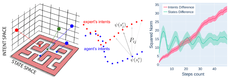
Figure 1: AILOT: Aligned Imitation Learning via Optimal Transport. Principal diagram for intents alignment. Left: Stage I: projection into intent space (denoted by $\psi$ in text) (only first $3$ principal components are shown). Middle: Stage II: computation of intrinsic rewards for offline RL, where $s_{i}^{a}$ and $s_{j}^{e}$ are the expert’s and the agent’s states, $P$ is the optimal transport transitions matrix; and the corresponding reward $r(s_{i}^{a})$ is a scaling transform of the product $\sum_{j}P_{ij}C_{ij}$ with some cost function $C$ defined on the intents pairs. Right: squared norm vs. steps count in the same trajectory for the states and the intents differences; It demonstrates that distance between intents is proportional to the total path length (steps count) between the states (AntMaze example is shown).

1 Introduction

Over the past years, offline learning has remained both the most logical and the most ambitious avenue for the development of RL. On the one hand, there is an ever-growing reservoir of sequential data, such as video, becoming available for training the decision-making RL agents. On the other hand, these immense data remain largely unlabeled and unstructured for gaining any valuable guidance in the form of rewards or action labels, stimulating the development of unsupervised and self-supervised methods Singh et al. (2020); Li et al. (2023); Sinha et al. (2022); Yu et al. (2022)

Drawing inspiration from the triumphant strategies employed in language-based foundational models, leveraging the vast reservoir of web-based data for offline RL indeed emerges as a promising avenue. However, the unresolved challenge persists in efficiently incorporating offline data into RL frameworks and processes Levine et al. (2020). Offline RL faces several challenges, such as distributional shift, slow convergence when the labels are unavailable, and the absence of known rewards which should be purposely designed for each separate task independently Kumar et al. (2021); Fujimoto et al. (2019).

A potential remedy to these challenges is found in Imitation Learning (IL), where the explicit reward functions are not needed. Instead, an imitating agent is trained to replicate the behavior of the expert. Behavior cloning (BC) Ross and Bagnell (2010) frames the IL problem akin to classical supervised learning, seeking to maximize the likelihood of the actions provided under the learner’s policy. Despite working well in simple environments, BC is prone to accumulating errors in states, coming from different distributions other than experts. Distribution matching is another promising IL paradigm, where approaches such as distribution correction estimation (”DICE”), including SMODICE Ma et al. (2022b), attempt to match state-occupancy measures between the imitator’s and the expert’s policies. Another notable approach is DEMODICE Kim et al. (2022), which uses state-action occupancy measures. One significant limitation of these methods is their requirement for a non-zero overlap between the supports of the agent’s performance dataset and the expert data.

Another promising avenue involves Computational Optimal Transport, a domain that has garnered significant popularity for addressing diverse machine learning tasks Peyré et al. (2019). Its applications span from domain adaptation to generative modeling Salimans et al. (2018); Rout et al. (2021); Korotin et al. (2022). It has proven to be efficient in weakly-supervised tasks Bespalov et al. (2022) and even for learning with one target sample and unlabelled source data Bespalov et al. (2020). To alleviate the necessity for manual reward engineering, Luo et al. (2023) leverages optimal transport theory. The approach automates the assignment of reward labels by establishing an optimal coupling between a select few high-quality expert demonstrations and the trajectories of the learning agent.

The absence of reward labels is not the sole challenge; obtaining access to expert actions can also be problematic. One potential remedy is to create a simulator Krylov et al. (2020); Saboo et al. (2021) that enables access to both actions and rewards. However, adopting such an approach entails substantial additional work. Consider a scenario where a thousand demonstrations of expert trajectories are available from videos, yet no rewards or action labels accompany them. In this work, we eliminate the requirement for either knowing the rewards or the action labels of the expert. By utilizing the Intention-Conditioned Value Function (ICVF) Ghosh et al. (2023), we showcase the potential to redefine the offline Imitation Learning (IL) problem as expert-guided. This guidance is achieved by contracting intent representations through the optimal transport. This framework allows for the complete discarding of the action labels, with the imitation now being centered around the proximity to the expert intentions. Given that an intention is a task-agnostic property, the learned representations prove to be sufficiently discriminative, providing valuable insights into the environment without relying on specific action or reward labels.

Our contribution is as follows:

• We introduce a new intrinsic reward function that depicts the dynamics in the environment and an offline imitation learning algorithm based on it.

• We report extensive comparison with previous works. Despite not having access to the expert’s action labels and ground truth rewards, we outperform the state-of-the-art models in the majority of benchmark datasets and show that our approach enables custom imitation even when agent’s data is a mix of random policies.

2 Related Works

In this study, we broaden the application of offline Reinforcement Learning (RL) to datasets that lack both the rewards and the action labels. Despite all the research effort on learning the intrinsic rewards for RL, most works assume either online RL setting Brown and Niekum (2019); Yu et al. (2020); Ibarz et al. (2018) or the unrealistic setup of possessing some annotated prior data. Moreover, the problem of learning and exploration in sparse-reward environments can be deemed as solved for online RL Li et al. (2023); Eysenbach et al. (2018); Lee et al. (2019); whereas, only a few works exist that consider the offline goal-conditioned setting with reward-free data Park et al. (2023); Zheng et al. (2023); Wang et al. (2023). The goal of our work is to extract guidance from observing the expert by finding optimal alignment of information-rich representations of imaginary goals between the expert and the agent in a shared latent space.

We build upon the approach introduced in Luo et al. (2023), extending it by finding a representative latent space. In Luo et al. (2023), the authors address the entropy-regularized Optimal Transport (OT) problem using Sinkhorn’s algorithm, focusing on expert and agent trajectories. By estimating the optimal coupling between these trajectories, every trajectory in the offline dataset can be annotated by intrinsic rewards.

A clear advantage of our method is its independence from the action and the reward labels, distinguishing it from the prior works Ho and Ermon (2016); Kim et al. (2022); Garg et al. (2021); Reddy et al. (2019); Pomerleau (1991); Yu et al. (2022). Additionally, the method seamlessly integrates with various downstream RL algorithms, providing flexibility in selecting the most suitable training approach. It is also essential to acknowledge a limitation of Luo et al. (2023): the method does not guarantee that geometry of unlabeled states distribution will be discriminative enough to provide right non-noisy reward signal through optimal transport. An alternative research direction, Calibrated Latent gUidancE (CLUE) Liu et al. (2023), introduces a parallel approach for deriving intrinsic rewards. In this study, the authors employ a conditional variational auto-encoder trained on both expert and agent transitions and compute the distance between the collapsed expert embedding and the agent trajectory. The expert embedding might not collapse into a single point in a multimodal expert dataset, requiring clustering to handle different skills. Unlike the CLUE method, our approach doesn’t need state-action labeled data, eliminating the need for action annotations.

3 Preliminaries

3.0.1 Problem Formulation

A standard Reinforcement Learning problem is defined as a Markov Decision Process (MDP) with tuple $\mathcal{M}=(\mathcal{S},\mathcal{A},p,r,\rho_{0},\gamma)$, where $\mathcal{S}\subset\mathbb{R}^{n}$ is the state space, $\mathcal{A}\subset\mathbb{R}^{m}$ is the action space, $p$ is a function describing transition dynamics in the environment $p$: $\mathcal{S}\times\mathcal{A}\rightarrow\mathcal{P}(\mathcal{S})$, $r:\mathcal{S}\times\mathcal{A}\rightarrow\mathbb{R}$ is a predefined extrinsic reward function, $\rho_{0}$ is an initial state distribution and $\gamma\in(0,1]$ is the discount factor. The objective is to learn policy $\pi_{\theta}(a|s):\mathcal{S}\rightarrow\mathcal{P}(\mathcal{A})$ that maximizes discounted cumulative return $\mathbb{E}[\sum^{\infty}_{t=0}\gamma^{t}r(s_{t},a_{t})]$. In contrast, offline RL assumes access to a pre-collected static dataset of transitions $\mathcal{D}=\{(s_{i},a_{i},s^{\prime}_{i},r_{i})\}^{n}_{i=1}$ while strictly prohibiting interaction with the environment. In this study, we assume access to a dataset of transitions without reward labels $\mathcal{D}_{a}=\{(s_{i},a_{i},s^{\prime}_{i})\}^{n}_{i=1}$, collected from $\mathcal{M}$, and a limited number of ground truth demonstrations from the expert policy without reward and action labels $\mathcal{D}_{e}=\{(s_{i},s^{\prime}_{i})\}^{m}_{i=1}$. These demonstrations are also collected from the same MDP ($\mathcal{M}$) and we assume that trajectories from $\mathcal{D}_{e}$ have high cumulative return. The primary objective is to determine a policy that closely emulates the behavior of the expert and thereby maximises the cumulative return.

3.0.2 ICVF Pretraining

Using pre-collected large unlabeled datasets in the form of prior data empowers agents to generalize their learned behaviors. Even in the absence of ground truth actions or rewards, agents can still acquire valuable insights into the environment dynamics and learn useful features. Recent work in the generalization of the value function, known as the Intention-Conditioned Value Function (ICVF), introduces the concepts of intentions and outcomes to replace traditional notions of actions and rewards Ghosh et al. (2023). ICVF fundamentally constructs a successor representation Dayan (1993), allowing the recovery of spatial correspondences within data based solely on observations. ICVF is task-agnostic, and the learned embeddings demonstrate sufficient discriminative capabilities to guide learning agents through intrinsic rewards toward expected behavior. Formally, considering two states from an offline dataset $s,s_{+}\in\mathcal{D}=\mathcal{D}_{a}\bigcup\mathcal{D}_{e}$, ICVF is defined as:

$$V(s,s_{+},z)=\sum_{t\geq 0}\gamma^{t}\mathbb{E}_{P_{z}}\left[\mathbb{I}[s_{t}=s_{+}]-1\,\big{|}\,s_{0}=s,z\right].$$ (1)

Let $P_{\mathcal{D}}(s_{t+1}|s_{t})$ denote the empirical transition probability in the dataset $\mathcal{D}$. The corresponding transition matrix of the Markov process is

$$P_{z}(s_{t+1}|s_{t})=\frac{\pi(z|s_{t+1},s_{t})}{\pi(z|s_{t})}P_{\mathcal{D}}(s_{t+1}|s_{t}).$$ (2)

ICVF estimates an average path length between states $s$ and $s_{+}$ (with a negative sign), conditioning on guidance of a latent variable $z$, defined as an intent of another state $\psi(s_{z})$. The intents policy $\pi(z|s_{z},s)$ implicitly (by means of implicit Q-learning method Kostrikov et al. (2021)) minimizes total step count between $s$ and $s_{z}$ from the same trajectory:

$$\min_{\pi,\psi}\mathbb{E}_{\mathcal{D}}(-1)\log\pi(\psi(s_{z})|s_{z},s)V(s,s_{z},\psi(s_{z})).$$ (3)

As a part of ICVF procedure, the value function is parametrized by three neural networks in the following decomposed format:

$$V(s,s_{+},z)=\phi(s)^{T}T(z)\psi(s_{+}).$$ (4)

We observed that the $\psi$ mapping itself (without $\phi$ and $T$) serves as a good estimate for the distances between the states of the environment. In the Experiments section below, we will empirically support this, showing that squared distance $d^{2}(s_{t+k},s_{t})=\|\psi(s_{t+k})-\psi(s_{t})\|^{2}$ is roughly a linear function of the steps count between the states ($k$).

4 Method

We extend the approach by Luo et al. Luo et al. (2023) to compute intrinsic rewards through an optimal transport. For two trajectories $\{s^{a}_{i}\}_{i=1}^{T_{a}}$ and $\{s^{e}_{j}\}_{j=1}^{T_{e}}$, the optimal transition matrix is given by solving the entropy-regularized OT problem:

$$P^{*}=\underset{P\in\Pi[T_{a},T_{e}]}{\arg\min}\left\{\sum_{ij}P_{ij}C_{ij}+\varepsilon\sum_{ij}P_{ij}\log P_{ij}\right\},$$ (5)

where $C_{ij}=c(s^{a}_{i},s^{a}_{i+k},s^{e}_{j},s^{e}_{j+k})$ is some cost function with parameter $k>0$ and $P$ has the following marginal distributions $\forall i,j$: $\sum_{j=1}^{T_{e}}P_{ij}=1/T_{a},\quad\sum_{i=1}^{T_{a}}P_{ij}=1/T_{e}$. By finding the optimal matrix $P^{*}$, we can determine the reward for each state of the trajectory $\{s^{a}_{i}\}_{i=1}^{T_{a}}$ as

$$r(s_{i}^{a})=A\exp\left(-\tau T_{a}\sum_{j=j_{1}}^{T_{e}}P^{*}_{ij}C_{ij}\right),$$ (6)

where

$$j_{1}=\arg\min_{j}C_{1j},$$ (7)

the exponent function with the hyperparameters $A$ and $\tau$ serves as an additional scaling factor to diminish the impact of the states with a large total cost. The negative sign ensures that, in the process of maximizing the sum of rewards, we are effectively minimizing the optimal transport (OT) distance.

Algorithm 1 AILOT Training

Input: $\mathcal{D}_{e}=\{\mathcal{T}^{e}_{i}\}^{K}_{i=1}$ – expert trajectories (states only);
$\mathcal{D}_{a}=\{\mathcal{T}^{a}_{i}\}^{L}_{i=1}$ – reward-free offline RL dataset
Parameters: $A$, $\tau$ – scaling, $k$ – shift in intents pair, $\varepsilon$ – OT entropy coefficient

1:  Let rewards $=$ List().

2:  Train $\psi$ intents mapping by ICVF procedure.

3:  for  $\mathcal{T}^{a}=\{s^{a}_{i}\}$ in $\mathcal{D}_{a}$ do

4:     Let $R=$ Array().

5:     for $\mathcal{T}^{e}=\{s^{e}_{j}\}$ in $\mathcal{D}_{e}$ do

6:        Compute cost matrix $C$ by expression (8);

7:        Let $j_{1}={\arg\min}_{j}C_{1j}$;

8:        Solve OT$\left(\{s^{a}_{i}\}_{i=1}^{T_{a}},\,\{s^{e}_{j}\}_{j=j_{1}}^{T_{e}}\right)$ and obtain $P^{*}$;

9:        Compute rewards $\{r(s^{a}_{i})\}_{i=1}^{T_{a}}$ by expression (6);

10:        Append $\{r(s^{a}_{i})\}_{i=1}^{T_{a}}$ to $R$.

11:     end for

12:     For each $i$ append $r_{i}=\min_{t}R_{ti}$ to rewards.

13:  end for

14:  return rewards

We proceed to estimate the transition matrix $P^{*}$ between each trajectory of the agent and the expert’s demonstrations (which may consist of one or more trajectories). For enhanced alignment, we selectively consider the tail of the expert’s trajectory $j_{1},\ldots,T_{e}$, focusing on the nearest first states to the agent’s starting position according to the cost matrix $C$. The maximum reward is selected across different trajectories when the expert provides multiple trajectories. The aggregated rewards for each trajectory of the agent are then incorporated into the offline dataset for subsequent RL training, with the policy trained by the IQL offline RL algorithm Kostrikov et al. (2021). A comprehensive recipe for the rewards computation procedure is shown in Algorithm 1.

In contrast to the OTR method by Luo et al. Luo et al. (2023) that computes distances directly between states, our approach measures differences between intents. Intents are such state representations that account for the temporal path length between the states in the environment. Specifically, we use the following cost matrix:

$$C_{ij}=\|\psi(s^{a}_{i})-\psi(s^{e}_{j})\|^{2}+\|\psi(s^{a}_{i+k})-\psi(s^{e}_{j+k})\|^{2}.$$ (8)

The inclusion of the second term in the cost is necessary for an ordered comparison of the trajectories. Hence, during training, we enforce the distribution of the agent’s intent pairs to converge to the empirical measure of the intent pairs of the expert.

Dataset	IQ-Learn	SQIL	ORIL	SMODICE	AILOT
halfcheetah-medium-v2	$21.7$ $\pm\>1.5$	$24.3$ $\pm\>2.7$	$56.8$ $\pm\>1.2$	$42.4$ $\pm\>0.6$	$47.7$ $\pm\>0.2$
halfcheetah-medium-replay-v2	$6.7$ $\pm\>1.8$	$43.8$ $\pm\>1.0$	$46.2$ $\pm\>1.1$	$38.3$ $\pm\>2.0$	$42.4$ $\pm\>0.2$
halfcheetah-medium-expert-v2	$2.0$ $\pm\>0.4$	$6.7$ $\pm\>1.2$	$48.7$ $\pm\>2.4$	$81.0$ $\pm\>2.3$	$92.4$ $\pm\>1.5$
hopper-medium-v2	$29.6$ $\pm\>5.2$	$66.9$ $\pm\>5.1$	$96.3$ $\pm\>0.9$	$54.8$ $\pm\>1.2$	$82.2$ $\pm\>5.6$
hopper-medium-replay-v2	$23.0$ $\pm\>9.4$	$98.6$ $\pm\>0.7$	$56.7$ $\pm\>12.9$	$30.4$ $\pm\>1.2$	$98.7$ $\pm\>0.4$
hopper-medium-expert-v2	$9.1$ $\pm\>2.2$	$13.6$ $\pm\>9.6$	$25.1$ $\pm\>12.8$	$82.4$ $\pm\>7.7$	$103.4$ $\pm\>5.3$
walker2d-medium-v2	$5.7$ $\pm\>4.0$	$51.9$ $\pm\>11.7$	$20.4$ $\pm\>13.6$	$67.8$ $\pm\>6.0$	$78.3$ $\pm\>0.8$
walker2d-medium-replay-v2	$17.0$ $\pm\>7.6$	$42.3$ $\pm\>5.8$	$71.8$ $\pm\>9.6$	$49.7$ $\pm\>4.6$	$77.5$ $\pm\>3.1$
walker2d-medium-expert-v2	$7.7$ $\pm\>2.4$	$18.8$ $\pm\>13.1$	$11.6$ $\pm\>14.7$	$94.8$ $\pm\>11.1$	$110.2$ $\pm\>1.2$
D4RL Locomotion total	$122.5$	$366.9$	$433.6$	$541.6$	$732.8$

Dataset	IQL	OTR	CLUE	AILOT
halfcheetah-medium-v2	$47.4$ $\pm\>0.2$	$43.3$ $\pm\>0.2$	$45.6$ $\pm\>0.3$	$47.7$ $\pm\>0.35$
halfcheetah-medium-replay-v2	$44.2$ $\pm\>1.2$	$41.3$ $\pm\>0.6$	$43.5$ $\pm\>0.5$	$42.4$ $\pm\>0.8$
halfcheetah-medium-expert-v2	$86.7$ $\pm\>5.3$	$89.6$ $\pm\>3.0$	$91.4$$\pm\>2.1$	$92.4$ $\pm\>1.54$
hopper-medium-v2	$66.2$ $\pm\>5.7$	$78.7$ $\pm\>5.5$	$78.3$ $\pm\>5.4$	$82.2$$\pm\>5.6$
hopper-medium-replay-v2	$94.7$ $\pm\>8.6$	$84.8$ $\pm\>2.6$	$94.3$ $\pm\>6.0$	$98.7$ $\pm\>0.4$
hopper-medium-expert-v2	$91.5$ $\pm\>14.3$	$93.2$ $\pm\>20.6$	$96.5$ $\pm\>14.7$	$103.4$ $\pm\>5.3$
walker2d-medium-v2	$78.3$ $\pm\>8.7$	$79.4$ $\pm\>1.4$	$80.7$ $\pm\>1.5$	$78.3$$\pm\>0.8$
walker2d-medium-replay-v2	$73.8$ $\pm\>7.1$	$66.0$ $\pm\>6.7$	$76.3$ $\pm\>2.8$	$77.5$ $\pm\>3.1$
walker2d-medium-expert-v2	$109.6$$\pm\>1.0$	$109.3$ $\pm\>0.8$	$109.3$ $\pm\>2.1$	$110.2$ $\pm\>1.2$
D4RL Locomotion total	$692.4$	$685.6$	$714.5$	$732.8$

Table 1: Normalized scores (mean $\pm$ standard deviation) of AILOT on MuJoco locomotion tasks, compared to baselines. For OTR, CLUE, and AILOT, the results are given for $K=1$ number of expert trajectories. The highest scores are highlighted.

Dataset	IQL	OTR	CLUE	AILOT
umaze-v2	$88.7$	$81.6$ $\pm\>7.3$	$92.1$ $\pm\>3.9$	$93.5$ $\pm\>4.8$
umaze-diverse-v2	$67.5$	$70.4$ $\pm\>8.9$	$68.0$ $\pm\>11.2$	$63.4$ $\pm\>7.6$
medium-play-v2	$72.9$	$73.9$ $\pm\>6.0$	$75.3$ $\pm\>6.3$	$71.3$ $\pm\>5.2$
medium-diverse-v2	$72.1$	$72.5$ $\pm\>6.9$	$74.6$ $\pm\>7.5$	$75.5$ $\pm\>7.4$
large-play-v2	$43.2$	$49.7$ $\pm\>6.9$	$55.8$$\pm\>7.7$	$57.6$ $\pm\>6.6$
large-diverse-v2	$46.9$	$48.1$ $\pm\>7.9$	$49.9$ $\pm\>6.9$	$66.6$ $\pm\>3.1$
AntMaze-v2 total	$391.3$	$396.2$	$415.7$	$427.9$

Dataset	IQL	OTR	CLUE	AILOT
door-cloned-v0	$1.6$	$0.01$ $\pm\>0.01$	$0.02$ $\pm\>0.01$	$0.05$ $\pm\>0.02$
door-human-v0	$4.3$	$5.9$$\pm\>2.7$	$7.7$ $\pm\>3.9$	$7.9$ $\pm\>3.2$
hammer-cloned-v0	$2.1$	$0.9$$\pm\>0.3$	$1.4$ $\pm\>1.0$	$1.6$ $\pm\>0.1$
hammer-human-v0	$1.4$	$1.8$$\pm\>1.4$	$1.9$ $\pm\>1.2$	$1.8$ $\pm 1.3$
pen-cloned-v0	$37.3$	$46.9$$\pm\>20.9$	$59.4$ $\pm\>21.1$	$61.4$ $\pm\>19.5$
pen-human-v0	$71.5$	$66.8$$\pm\>21.2$	$82.9$ $\pm\>20.2$	$89.4$ $\pm\>0.1$
relocate-cloned	-$0.2$	-$0.24$$\pm\>0.03$	-$0.23$ $\pm\>0.02$	-$0.20$ $\pm\>0.03$
relocate-human	$0.1$	$0.1$$\pm\>0.1$	$0.2$ $\pm\>0.3$	$0.28$ $\pm\>0.1$
Adroit-v0 total	$118.1$	$122.2$	$153.3$	$162.2$

Table 2: Normalized scores (mean $\pm$ standard deviation) of AILOT on Adroit and AntMaze tasks, compared to baselines. OTR, CLUE, and AILOT use IQL as offline RL baseline algorithm with only a single expert episode. The highest scores are highlighted.

5 Experiments

In the current section, we demonstrate performance of AILOT on several benchmarking tasks, make ablation study on varying number of provided expert demos and provide implementation details.

First, we empirically show the ability of proposed method to efficiently utilize expert demonstrations on sparse-rewards tasks (such as Antmaze and Adroit environments) and improve learning ability of offline RL algorithms by providing geometrically aware dense reward signal to agent’s transitions. Second, we evaluate how well AILOT performs in offline Imitation Learning (IL) setting, showing improved performance upon state-of-the art offline IL algorithms on MuJoco locomotion tasks. Moreover, for imitation learning, we include additional experiments with custom locomotion behaviors, e.g expert hopper performing backflip, when agent dataset consists of only completely random behaviors.

5.1 Implementation

Because our method provides intrinsic dense reward relabelling, any offline RL algorithm can be used afterwards to learn decision making policy, closely resembling expert behaviors. In all our experitiments we endow AILOT with Implicit Q-Learning (IQL), which is simple and robust offline RL algorithm.

We implement AILOT in JAX Bradbury et al. (2018) and use official implementations of both ICVF and IQL . Our code is written using Equinox library Kidger and Garcia (2021). In order to compute optimal couplings, we utilize efficient implementation of Sinkhorn algorithm Cuturi (2013) from OTT-JAX library Cuturi et al. (2022). We found that $200$ Sinkhorn solver iterations are enough to find optimal mapping and set $\epsilon=0.001$ as entropy regularization parameter. All hyperparameters for IQL on D4RL benchmarks are set to those recommended in original paper to ensure reproducibility. We use default latent dimension of $256$ for ICVF embeddings pretraining across all benchmarks and set other hyperparameters as in original paper. In order to maintain rewards in a reasonable range, they are scaled by exponential function as written in Equation 6 with $A=5,\tau=0.5$ for MuJoco and AntMaze tasks and $A=5,\tau=10$ for Adroit. We found that lookahead parameter in Equation 8 works best for $k=2$. Results are evaluated across 10 random seeds and 10 evaluation episodes for each seed in order to be consistent with previous works.

(a)

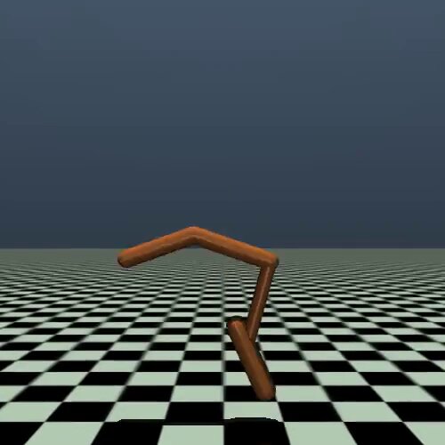
(b)

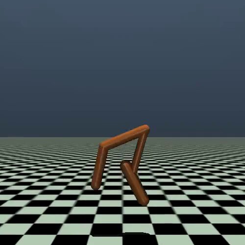
(c)

(d)

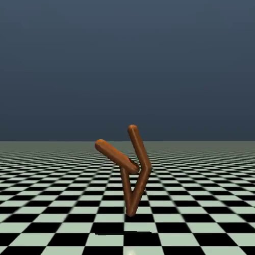
(e)

(f)

Figure 2: Expert demonstrator Hopper performs a backflip.

(a)

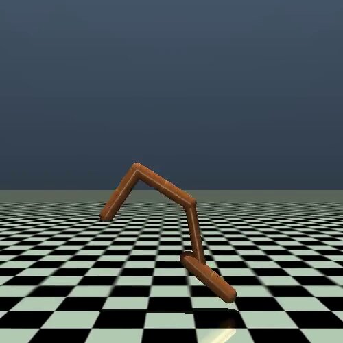
(b)

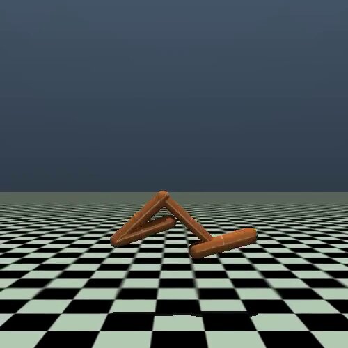
(c)

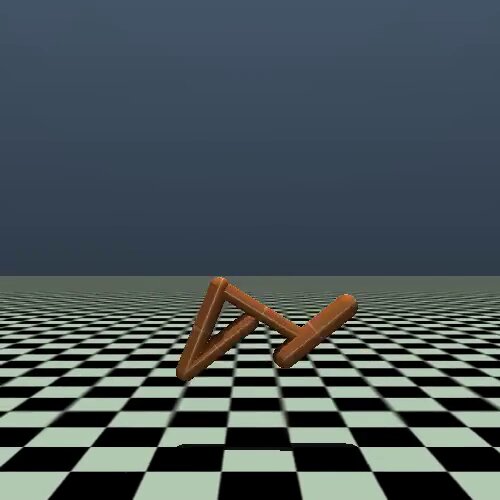
(d)

(e)

(f)

Figure 3: Hopper agent successfully performs imitation of backlip from the observations via AILOT.

Figure 4: Expert demonstrator HalfCheetah performs an upward standing.

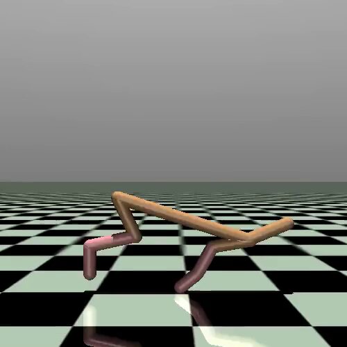
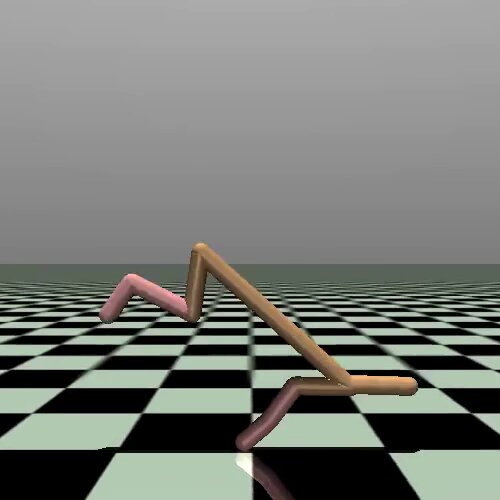
Figure 5: HalfCheetah agent successfully performs imitation of standing upwards from the observations via AILOT.

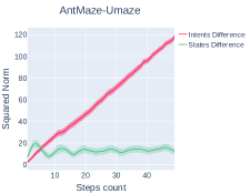
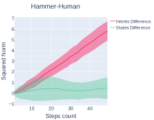
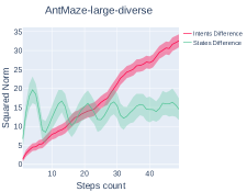
Figure 6: The squared norm of states and intents differences, depending on the total steps count between the states in the same trajectory. The average squared norm of intents differences has a near-linear dependence on the steps count. The squared norm in the state space is not a monotone function, which is less efficient for training an imitating agent.

5.2 Baselines

Performance of AILOT + IQL is compared to the following algorithms:

• IQL Kostrikov et al. (2021) is state-of-the-art offline RL algorithm, which avoids querying out of the distribution actions by viewing value function as a random variable, where upper bound of uncertanity is controlled through expectile of distribution. In our experiments, evaluation is made using ground-truth reward from D4RL tasks.

• OTR Luo et al. (2023) is a reward function algorithm, where reward signal is based on optimal transport distance between states of expert demonstration and reward unlabeled dataset.

• CLUE Liu et al. (2023) learns VAE calibrated latent space of both expert and agent state-action transitions, where intrinsic rewards can be defined as distance between agent and averaged expert transition representations.

• IQ-Learn Garg et al. (2021) is an imitation learning algorithm, which implicitly encodes into learned inverse Q-function rewards and policy from expert data.

• SQIL Reddy et al. (2019) proposes to learn soft Q-function by setting expert transitions to one and for non-expert transitions to zero.

• ORIL Zolna et al. (2020) utilizes discriminator network which distinguishes between optimal and suboptimal data in mixed dataset to provide reward relabelling through learned discriminator.

• SMODICE Ma et al. (2022a) offline state occupancy matching algorithm, which solves the problem of IL from observations through state divergence minimization by utilizing dual formulation of value function.

5.3 Results

In this section, we show the results for the following offline RL settings: (1) the imitation setting, where the goal is to mimic the behavior as closely as possible given the expert demonstrations; (2) the sparsified reward tasks, where the reward of one is given only when the agent reaches the goal state. We show that the rewards obtained through AILOT relabelling in both settings are descriptive enough to recover the demonstrated policy.

Dataset	OTR, $K=1$	AILOT, $K=1$	OTR, $K=5$	AILOT, $K=5$
halfcheetah-medium-v2	$43.3$ $\pm\>0.2$	$47.7$$\pm\>0.2$	$45.2$$\pm\>0.2$	$46.6$$\pm\>0.2$
halfcheetah-medium-replay-v2	$41.3$$\pm\>0.6$	$42.4$$\pm\>0.2$	$41.9$$\pm\>0.3$	$41.2$ $\pm\>0.5$
halfcheetah-medium-expert-v2	$89.6$ $\pm\>3.0$	$92.4$$\pm\>1.5$	$89.9$ $\pm\>1.9$	$92.4$ $\pm\>1.0$
hopper-medium-v2	$78.7$ $\pm\>5.5$	$82.2$$\pm\>5.6$	$79.5$ $\pm\>5.3$	$82.5$$\pm\>3.7$
hopper-medium-replay-v2	$84.8$ $\pm\>2.6$	$98.7$$\pm\>0.4$	$85.4$ $\pm\>1.7$	$97.4$ $\pm\>0.1$
hopper-medium-expert-v2	$93.2$ $\pm\>20.6$	$103.4$$\pm\>5.3$	$90.4$$\pm\>21.5$	$107.3$ $\pm\>5.6$
walker2d-medium-v2	$79.4$$\pm\>1.4$	$78.3$$\pm\>0.8$	$79.8$ $\pm\>1.4$	$80.9$ $\pm\>1.4$
walker2d-medium-replay-v2	$66.0$$\pm\>1.4$	$77.5$$\pm\>3.1$	$71.0$ $\pm\>5.0$	$76.9$ $\pm\>1.6$
walker2d-medium-expert-v2	$109.3$ $\pm\>0.8$	$110.2$$\pm\>1.2$	$109.4$ $\pm\>0.4$	$110.3$ $\pm\>0.4$
D4RL Locomotion total	$685.6$	$732.8$	$690.6$	$735.5$

Table 3: Normalized scores for D4RL locomotion tasks with $K=5$ expert trajectories. The highest scores are highlighted.

Offline Imitation Learning.

We compare AILOT performance on IL tasks in the offline setting. D4RL MuJoco locomotion datasets are used as the main source of offline data with the original reward signal and the action labels discarded, and the expert trajectories chosen for each task as the best episodes achieving maximal return. Results for D4RL locomotion tasks are presented in Table 1. AILOT achieves the best performance in $7$ out of $9$ benchmarks, when compared to OTR and CLUE. Note that, unlike the CLUE method, our algorithm does not rely on the action labels. Empirically, we confirm that the optimal geometrically aware map between the expert and the agent trajectories in the ICVF latent space gives reasonable guidance for the agent to learn properly.

We merge expert demos with unlabeled offline data and train ICVF on the resulting dataset, requiring only $\sim 250$k steps to provide task-agnostic useful spatial representations of states dynamics in the form of intents. Such ICVF representations can be used for finding optimal coupling between expert and agent transitions in the intents space, thus ‘pulling’ the agent towards the demonstrated behavior via intrinsic rewards as described in Section 4. We chose Euclidean distance as a measure of similarity in the intent latent space and perform exponential scaling of rewards according to Eq. (6) in order to maintain them in the appropriate range.

Also, we include additional imitation results when a custom demonstrations is provided, as in Figures 2 and 4, where the Hopper expert makes a backward flip and the HalfCheetah stands upwards respectively. Note that our agent’s dataset initially consists of only the random behaviors. Figures 3 and 5 show how the randomly initialized agent learns to recover the desired behavior through the AILOT relabelling.

Sparse-Reward Offline RL Tasks.

Next, we evaluate AILOT on several sparse D4RL benchmarks (namely, AntMaze-v2 and Adroit-v2). To obtain expert trajectories, we consider only those episodes that accomplish the goal task, dismissing all the others. As stated in the previous Section, ICVF provides structured representations in the latent space, making it easy to distinguish between any two distinct trajectories.

Table 2 compares the performance of AILOT+IQL to OTR+IQL,  CLUE+IQL, when only a single demonstration trajectory is available, and to the original IQL. We observe that AILOT outperforms the current state-of-the art results, with the hardest antmaze-large-diverse task showing the most remarkable margin. This proves the ability of AILOT to employ the expressive representations from ICVF through the optimal transport for functional learning in the sparse tasks as well.

5.4 Ablation Studies

Varying the number of expert trajectories.

We investigate whether performance of learned behavior tends to improve with increased number of provided expert trajectories. Table 3 shows overall performance for varying number of expert trajectories from $K=1$ to $K=5$ across OTR and AILOT. However, we observe that performance across both algorithms improves slightly. We make comparison with OTR here because it’s the most similar to ours (it also uses OT for reward labelling and IQL for RL problem solution). Still, AILOT achieves better normalized scores than OTR, thus proving that alignment in intents representation space improves intrinsic rewards labelling in comparison with similar rewards but with pairwise distances between original states.

Intents distance dependence on the steps count.

In the Method section, we have already mentioned that $\mathbb{E}_{t}\|\psi(s_{t+k})-\psi(s_{t})\|^{2}$ is near-linearly dependent on the steps count between the states ($k$). This important property plays a constructive role in the cost matrix in the OT problem (8), and ultimately, gives a good estimate of the distance between the trajectories. Empirical evidence of the near-linear dependence is presented in Figure 6. Here, we also show that the pairwise distances between the original states $\mathbb{E}_{t}\|s_{t+k}-s_{t}\|^{2}$ have no such feature and, thus, their direct use as a cost function is less preferable.

6 Discussion

In our work, we introduced a novel non-adversarial method for extracting expert’s reward function for offline imitation learning, called AILOT. We empirically show that it surpasses the state-of-the art results both in the sparse-reward RL tasks and in the imitation learning setting. Our method removes the traditional constraint, introduced in the previous offline imitation learning algorithms, where the action labels used to be a necessity. To the contrary, AILOT can mimic the expert behaviour without knowing its action labels, and without the ground truth rewards. Moreover, we show that the intrinsic rewards, distilled by AILOT, could be used to efficiently boost the performance of other offline RL algorithms, thanks to the proper alignment to the expert intentions via the optimal transport.

AILOT assumes there is a sufficient access to a large number of unlabeled trajectories of sub-optimal quality. In our work, we have focused on the expert behaviours, typically considered in the offline RL publications: popular synthetic environments with some comprehensible expert movements and, consequently, some sufficiently ‘intuitive’ intentions.

If, however, the expert has several goals or performs a vague action, the imitation efficiency could, of course, drop (because the expert intents may no longer be transparent to the agent). While such a trait would be on par with the way humans learn a certain skill by observing an adept, weighing the hierarchy of multiple possible intents in AILOT could prove useful to further regularize the learning dynamics in such uncertain scenarios. Notably, such an add-on could be also done in an unsupervised manner, so that the annotations would remain unneeded in the end-to-end implementation.

Another direction of future work is to venture into the cross-domain imitation. Based on the results observed here, it should be possible to generalize AILOT to handle the transition shift between the expert and the agent in the presence of larger mismatches pertinent to the different domains. ICVF is agnostic to the domain setting, making us believe that the cross-domain extension is feasible.

In conclusion, the development of AILOT sets a robust benchmark for future generalizations, enhancing ongoing research in crafting generalist agents with comprehensive knowledge distillation capabilities.

AILOT Flow Diagram

In this Appendix, we provide additional details about the experimental setup and the hyperparameters, along with short discussion on crucial differences from previous works. We also visualize some XMagical trajectories and the intents to show how AILOT manages to comprehend the goal of the expert in the offline RL setting.

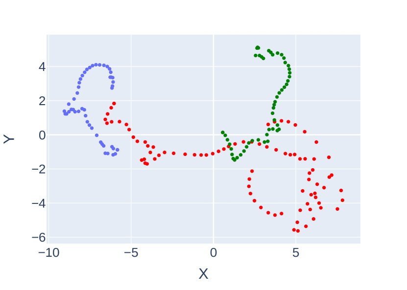
(a)

Figure 7: ICVF $\psi$ TSNE projections for three different trajectories from XMagical dataset.

Experimental Details

Hyperparameters

It should be noted that IQL incorporates its own rewards rescaling function within the dataset. We apply similar technique, using the reward scaling factor of

$$\frac{1000}{\mbox{max\_return}-\mbox{min\_return}}.$$

For MuJoco locomotion benchmarks and for AntMaze-v2, we subtract 1 from the rewards provided by AILOT. All the other parameters for IQL are kept intact. The other parameters are presented in Tables 4 and 5. For AntMaze tasks, the parameters are the same as for Mujoco, except for the expectile in IQL, which we set to $0.9$. ICVF pretraining executed for $250$k steps, since we found that it is enough for ICVF intentions to converge.

Algorithm	Hyperparameter	Value
IQL	Temperature	6
	Expectile	0.7
AILOT	$\tau$	0.5
	A	5
	Sinkhorn $\epsilon$	0.001
	k	2
ICVF	Pretraining steps	250k

Table 4: Hyperparameters for MuJoco tasks.

Algorithm	Hyperparameter	Value
IQL	Temperature	5
	Expectile	0.7
AILOT	$\tau$	10
	A	5
	Sinkhorn $\epsilon$	0.001
	k	2
ICVF	Pretraining steps	250k

Table 5: Hyperparameters for Adroit tasks.

Additional ICVF Plots

We include additional graphs, depicting the advantage of using ICVF for the initialization of intents. To prove this point, we provide additional low-dimensional projections of intents from $\psi$ for XMagical dataset. XMagical benchmark consists of four agents with different morphologies and frequently used to measure learning abilities of agent in cross-domain setting. Target goal is to Sweep 3 blocks towards pink zone on top. Each agent has it is own physics dynamics due to unique embodiment. The ground-truth reward is the amount of debris located at pink zone (denoted as $\mathbb{G}$) at the end of episode, i.e $\frac{1}{3}\sum^{3}_{i=1}\mathbb{I}\{b\in\mathbb{G}\}$. In Fig 8 we give results of how well AILOT performs imitation from data of other agents in offline setting for Mediumstick, trained on Lonsgstick, Shortstick.

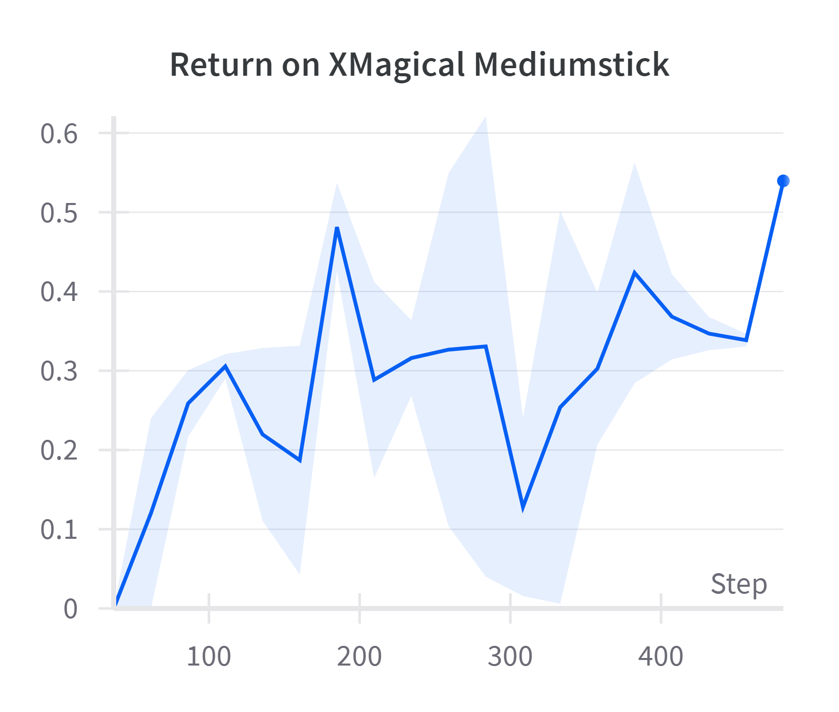
(a)

Figure 8: Mediumstick return by using AILOT from data of Shortstick and Longstick agents.

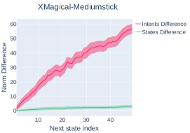
Figure 9: Mediumstick difference between intentions is linear, which corresponds to temporal consistency between their indices, while states difference flattens at some point.

Fig 12 shows intents difference between the corresponding states (top and below) for XMagical gripper agent. ICVF is lower for states which are similiar to each other. We also note that such crucial feature generalizes to cross-domain setting, thus paving a way towards finding a generalization of AILOT for cross-embodiment setting.

Visualizations of XMagical Trajectories

Fig 7 shows visualization of TSNE projection of ICVF $\psi$ for three different trajectories from Gripper environment. We observe that the geometry of learned features from $\psi$ is informative enough to clearly distinguish between trajectories and push one trajectory into the other by means of AILOT, so that the intrinsic rewards guide agent towards correct behavior. However, we should point out that it is hard to derive right conclusions from the low-dimensional projections alone, because such techniques usually distort learned distance information.

Moreover, Fig 13 shows $\psi$ TSNE projections for different XMagical agents. Despite having different morphologies, we observe that trajectories of different agents create clusters and similiar clusters correspond to similiar states visited by distinct agents.

Differences from Previous Approaches

AILOT provides guidance towards mimicking expert behavior by means of intrinsic rewards in offline setting. The closest works are OTR and CLUE. As was stated in main text body, our approach significantly differs from them in the sense of considering intrinsic rewards guidance from intentions perspective. In contrast, OTR considers optimal transport distance in the original state space, which is very noisy and lacks spatial information between different states as shown in Fig 9. CLUE uses distance between expert and agent behaviors in VAE latent space instead. However, in order to provide discriminative distance signal, expert embeddings are collapsed towards single point, completely destroying useful information about dependencies between states and thus pushing agent towards average expert. On the contrary, AILOT leverages spatial representations of states from ICVF and optimal transport in order to align expert and agent intent measures, thus providing much clearer signal from expert in the form of rewards.

Code

We commit to make our code public upon acceptance of the paper to the conference. Along with ICVF checkpoints used for optimal transport alignment.

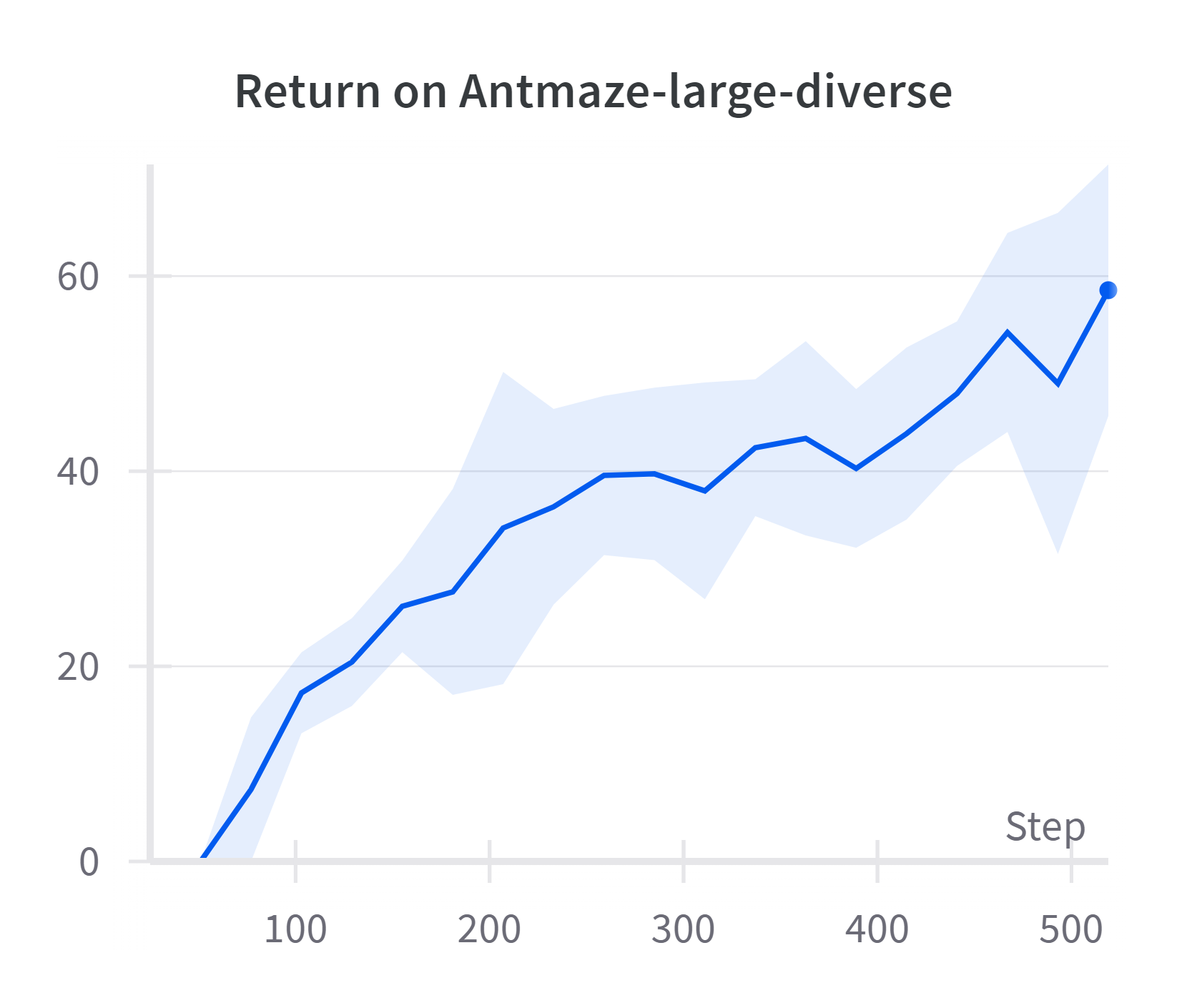
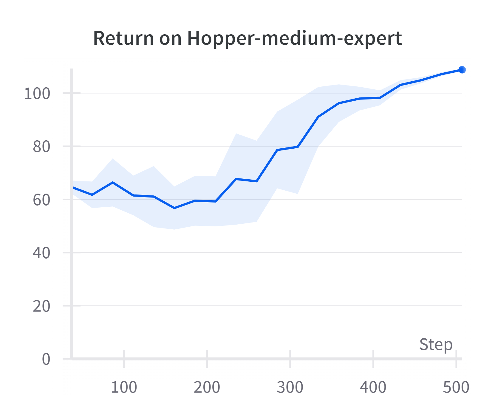
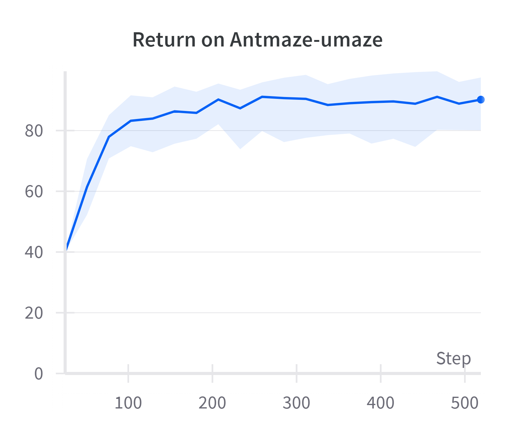
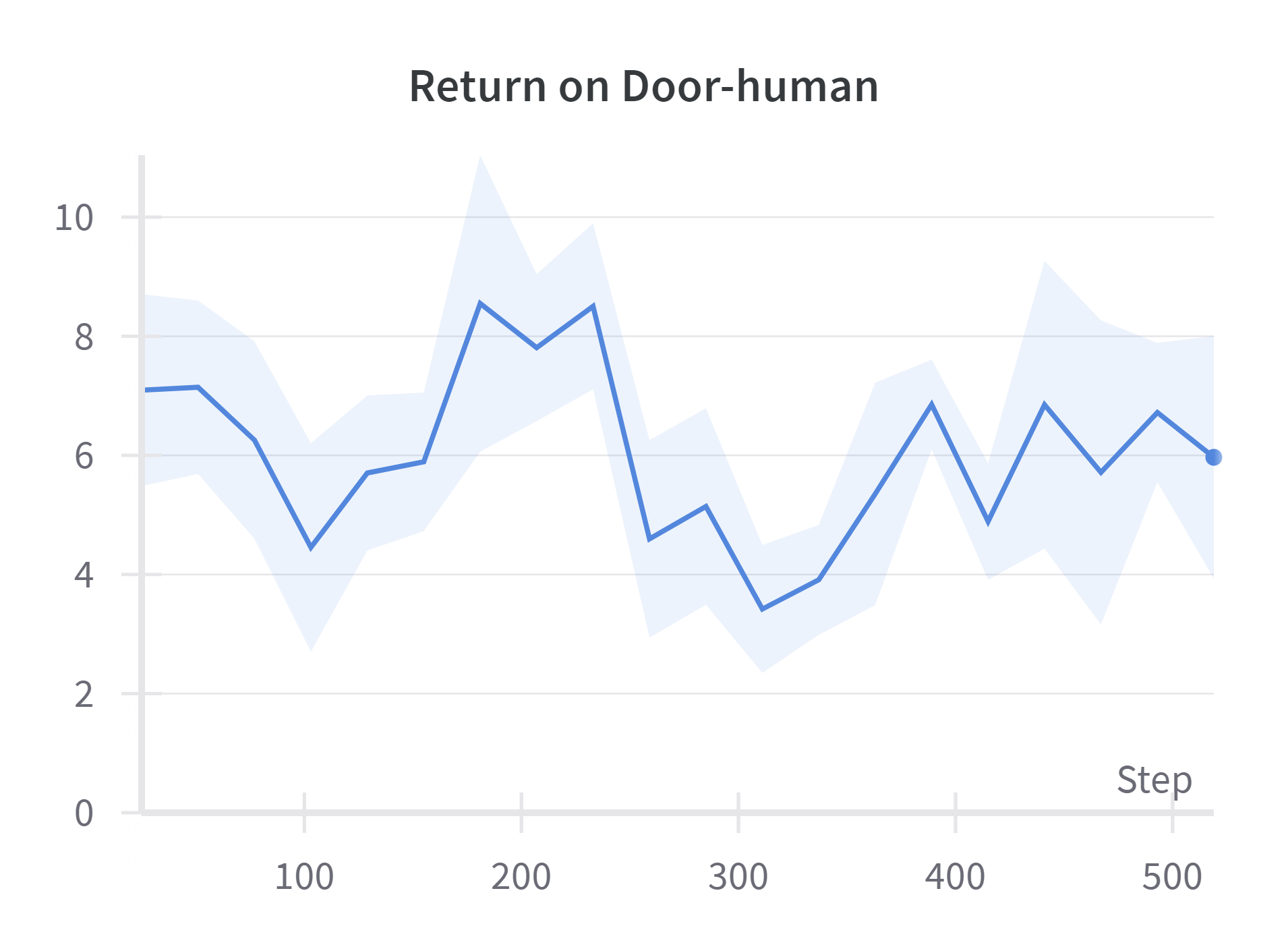
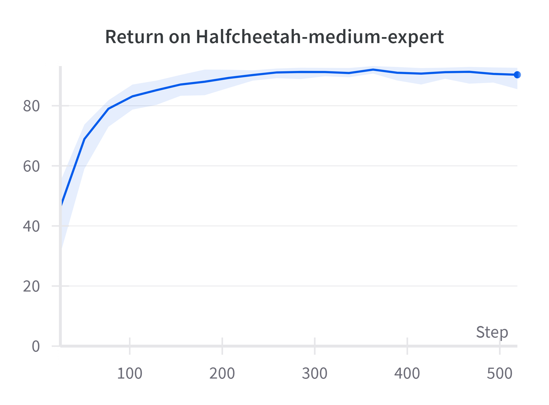
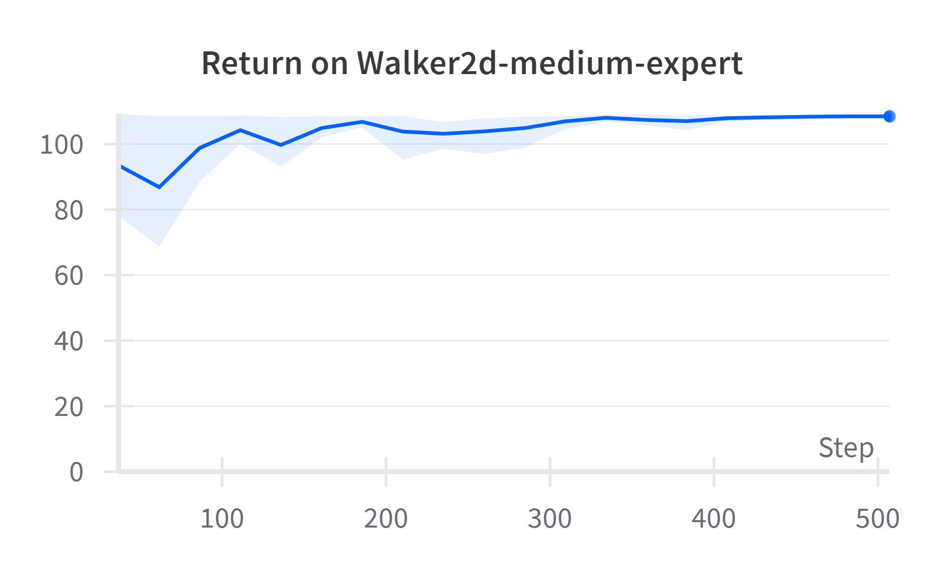
Figure 10: Return curves for different benchmarks during learning of AILOT + IQL

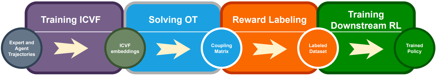
Figure 11: Flow diagram of intrinsic reward guidance via AILOT.

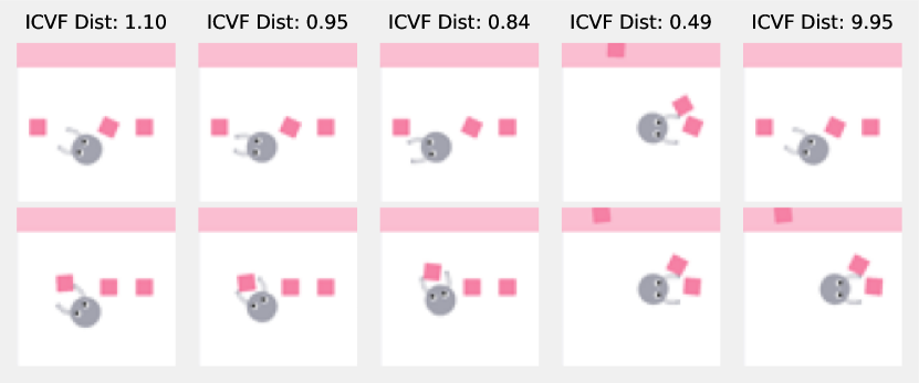
(a)

Figure 12: Visualizations of two different trajectories of Gripper agent with corresponding $L^{2}$ distances between the intents.

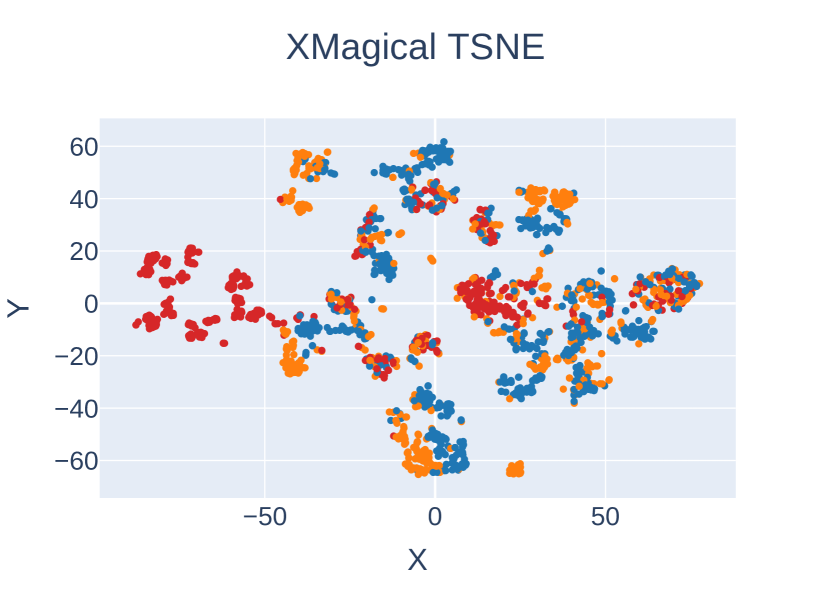
(a)

Figure 13: ICVF visualizations of random samples from XMagical sticks agent’s datasets. Red: Longstick agent. Orange: Mediumstick agent. Blue: Shortstick agent.

References

- Bespalov et al. [2020] Iaroslav Bespalov, Nazar Buzun, and Dmitry V. Dylov. Brulé: Barycenter-regularized unsupervised landmark extraction. Pattern Recognit., 131:108816, 2020.
- Bespalov et al. [2022] Iaroslav Bespalov, Nazar Buzun, Oleg Kachan, and Dmitry V. Dylov. Lambo: Landmarks augmentation with manifold-barycentric oversampling. IEEE Access, 10:117757–117769, 2022.
- Bradbury et al. [2018] James Bradbury, Roy Frostig, Peter Hawkins, Matthew James Johnson, Chris Leary, Dougal Maclaurin, George Necula, Adam Paszke, Jake VanderPlas, Skye Wanderman-Milne, and Qiao Zhang. JAX: composable transformations of Python+NumPy programs, 2018.
- Brown and Niekum [2019] Daniel S Brown and Scott Niekum. Deep bayesian reward learning from preferences. arXiv preprint arXiv:1912.04472, 2019.
- Cuturi et al. [2022] Marco Cuturi, Laetitia Meng-Papaxanthos, Yingtao Tian, Charlotte Bunne, Geoff Davis, and Olivier Teboul. Optimal transport tools (ott): A jax toolbox for all things wasserstein. arXiv preprint arXiv:2201.12324, 2022.
- Cuturi [2013] Marco Cuturi. Sinkhorn distances: Lightspeed computation of optimal transport. Advances in neural information processing systems, 26, 2013.
- Dayan [1993] Peter Dayan. Improving generalization for temporal difference learning: The successor representation. Neural computation, 5(4):613–624, 1993.
- Eysenbach et al. [2018] Benjamin Eysenbach, Abhishek Gupta, Julian Ibarz, and Sergey Levine. Diversity is all you need: Learning skills without a reward function. arXiv preprint arXiv:1802.06070, 2018.
- Fujimoto et al. [2019] Scott Fujimoto, David Meger, and Doina Precup. Off-policy deep reinforcement learning without exploration. In International conference on machine learning, pages 2052–2062. PMLR, 2019.
- Garg et al. [2021] Divyansh Garg, Shuvam Chakraborty, Chris Cundy, Jiaming Song, and Stefano Ermon. Iq-learn: Inverse soft-q learning for imitation. Advances in Neural Information Processing Systems, 34:4028–4039, 2021.
- Ghosh et al. [2023] Dibya Ghosh, Chethan Anand Bhateja, and Sergey Levine. Reinforcement learning from passive data via latent intentions. In International Conference on Machine Learning, pages 11321–11339. PMLR, 2023.
- Ho and Ermon [2016] Jonathan Ho and Stefano Ermon. Generative adversarial imitation learning, 2016.
- Ibarz et al. [2018] Borja Ibarz, Jan Leike, Tobias Pohlen, Geoffrey Irving, Shane Legg, and Dario Amodei. Reward learning from human preferences and demonstrations in atari. Advances in neural information processing systems, 31, 2018.
- Kidger and Garcia [2021] Patrick Kidger and Cristian Garcia. Equinox: neural networks in JAX via callable PyTrees and filtered transformations. Differentiable Programming workshop at Neural Information Processing Systems 2021, 2021.
- Kim et al. [2022] Geon-Hyeong Kim, Seokin Seo, Jongmin Lee, Wonseok Jeon, Hyeongjoo Hwang, Hongseok Yang, and Kee-Eung Kim. Demodice: Offline imitation learning with supplementary imperfect demonstrations. 01 2022.
- Korotin et al. [2022] Alexander Korotin, Daniil Selikhanovych, and Evgeny Burnaev. Neural optimal transport. arXiv preprint arXiv:2201.12220, 2022.
- Kostrikov et al. [2021] Ilya Kostrikov, Ashvin Nair, and Sergey Levine. Offline reinforcement learning with implicit q-learning. 2021.
- Krylov et al. [2020] Dmitrii Krylov, Dmitry V. Dylov, and Michael Rosenblum. Reinforcement learning for suppression of collective activity in oscillatory ensembles. Chaos: An Interdisciplinary Journal of Nonlinear Science, 30(3), March 2020.
- Kumar et al. [2021] Aviral Kumar, Joey Hong, Anikait Singh, and Sergey Levine. Should i run offline reinforcement learning or behavioral cloning? In International Conference on Learning Representations, 2021.
- Lee et al. [2019] Lisa Lee, Benjamin Eysenbach, Emilio Parisotto, Eric Xing, Sergey Levine, and Ruslan Salakhutdinov. Efficient exploration via state marginal matching. arXiv preprint arXiv:1906.05274, 2019.
- Levine et al. [2020] Sergey Levine, Aviral Kumar, George Tucker, and Justin Fu. Offline reinforcement learning: Tutorial, review, and perspectives on open problems. arXiv preprint arXiv:2005.01643, 2020.
- Li et al. [2023] Qiyang Li, Jason Zhang, Dibya Ghosh, Amy Zhang, and Sergey Levine. Accelerating exploration with unlabeled prior data. arXiv preprint arXiv:2311.05067, 2023.
- Liu et al. [2023] Jinxin Liu, Lipeng Zu, Li He, and Donglin Wang. Clue: Calibrated latent guidance for offline reinforcement learning, 2023.
- Luo et al. [2023] Yicheng Luo, Zhengyao Jiang, Samuel Cohen, Edward Grefenstette, and Marc Peter Deisenroth. Optimal transport for offline imitation learning. arXiv preprint arXiv:2303.13971, 2023.
- Ma et al. [2022a] Yecheng Ma, Andrew Shen, Dinesh Jayaraman, and Osbert Bastani. Versatile offline imitation from observations and examples via regularized state-occupancy matching. In International Conference on Machine Learning, pages 14639–14663. PMLR, 2022.
- Ma et al. [2022b] Yecheng Jason Ma, Andrew Shen, Dinesh Jayaraman, and Osbert Bastani. Versatile offline imitation from observations and examples via regularized state-occupancy matching, 2022.
- Park et al. [2023] Seohong Park, Dibya Ghosh, Benjamin Eysenbach, and Sergey Levine. Hiql: Offline goal-conditioned rl with latent states as actions. arXiv preprint arXiv:2307.11949, 2023.
- Peyré et al. [2019] Gabriel Peyré, Marco Cuturi, et al. Computational optimal transport: With applications to data science. Foundations and Trends® in Machine Learning, 11(5-6):355–607, 2019.
- Pomerleau [1991] Dean A. Pomerleau. Efficient training of artificial neural networks for autonomous navigation. Neural Computation, 3(1):88–97, 1991.
- Reddy et al. [2019] Siddharth Reddy, Anca D Dragan, and Sergey Levine. Sqil: Imitation learning via reinforcement learning with sparse rewards. arXiv preprint arXiv:1905.11108, 2019.
- Ross and Bagnell [2010] Stéphane Ross and Drew Bagnell. Efficient reductions for imitation learning. In Proceedings of the thirteenth international conference on artificial intelligence and statistics, pages 661–668. JMLR Workshop and Conference Proceedings, 2010.
- Rout et al. [2021] Litu Rout, Alexander Korotin, and Evgeny Burnaev. Generative modeling with optimal transport maps. arXiv preprint arXiv:2110.02999, 2021.
- Saboo et al. [2021] Krishnakant Saboo, Anirudh Choudhary, Yurui Cao, Gregory Worrell, David Jones, and Ravishankar Iyer. Reinforcement learning based disease progression model for alzheimer’s disease. In M. Ranzato, A. Beygelzimer, Y. Dauphin, P.S. Liang, and J. Wortman Vaughan, editors, Advances in Neural Information Processing Systems, volume 34, pages 20903–20915. Curran Associates, Inc., 2021.
- Salimans et al. [2018] Tim Salimans, Han Zhang, Alec Radford, and Dimitris Metaxas. Improving gans using optimal transport. arXiv preprint arXiv:1803.05573, 2018.
- Singh et al. [2020] Avi Singh, Albert Yu, Jonathan Yang, Jesse Zhang, Aviral Kumar, and Sergey Levine. Cog: Connecting new skills to past experience with offline reinforcement learning. arXiv preprint arXiv:2010.14500, 2020.
- Sinha et al. [2022] Samarth Sinha, Ajay Mandlekar, and Animesh Garg. S4rl: Surprisingly simple self-supervision for offline reinforcement learning in robotics. In Conference on Robot Learning, pages 907–917. PMLR, 2022.
- Wang et al. [2023] Mianchu Wang, Rui Yang, Xi Chen, and Meng Fang. Goplan: Goal-conditioned offline reinforcement learning by planning with learned models. arXiv preprint arXiv:2310.20025, 2023.
- Yu et al. [2020] Xingrui Yu, Yueming Lyu, and Ivor Tsang. Intrinsic reward driven imitation learning via generative model. In International conference on machine learning, pages 10925–10935. PMLR, 2020.
- Yu et al. [2022] Tianhe Yu, Aviral Kumar, Yevgen Chebotar, Karol Hausman, Chelsea Finn, and Sergey Levine. How to leverage unlabeled data in offline reinforcement learning. In International Conference on Machine Learning, pages 25611–25635. PMLR, 2022.
- Zheng et al. [2023] Chongyi Zheng, Ruslan Salakhutdinov, and Benjamin Eysenbach. Contrastive difference predictive coding. arXiv preprint arXiv:2310.20141, 2023.
- Zolna et al. [2020] Konrad Zolna, Alexander Novikov, Ksenia Konyushkova, Caglar Gulcehre, Ziyu Wang, Yusuf Aytar, Misha Denil, Nando de Freitas, and Scott Reed. Offline learning from demonstrations and unlabeled experience. arXiv preprint arXiv:2011.13885, 2020.