Towards Trustworthy Reranking:
A Simple yet Effective Abstention Mechanism

Abstract

Neural Information Retrieval (NIR) has significantly improved upon heuristic-based IR systems. Yet, failures remain frequent, the models used often being unable to retrieve documents relevant to the user’s query. We address this challenge by proposing a lightweight abstention mechanism tailored for real-world constraints, with particular emphasis placed on the reranking phase. We introduce a protocol for evaluating abstention strategies in a black-box scenario, demonstrating their efficacy, and propose a simple yet effective data-driven mechanism. We provide open-source code for experiment replication and abstention implementation, fostering wider adoption and application in diverse contexts.

1 Introduction

In recent years, Neural Information Retrieval (NIR) has emerged as a promising approach to addressing the challenges of Information Retrieval (IR) on various tasks Guo et al. (2016); Mitra and Craswell (2017); Zhao et al. (2022). Central to the NIR paradigm are the pivotal stages of retrieval and reranking Robertson et al. (1995); Ni et al. (2021); Neelakantan et al. (2022), which collectively play a fundamental role in shaping the performance and outcomes of IR systems Thakur et al. (2021). While the objective of the retrieval stage is to efficiently fetch candidate documents from a vast corpus based on a user’s query (frequentist Ramos et al. (2003); Robertson et al. (2009) or bi-encoder-based approaches Karpukhin et al. (2020)), reranking aims at reordering these retrieved documents in a slower albeit more effective way, using more sophisticated techniques (bi-encoder- or cross-encoder-based Nogueira and Cho (2019); Khattab and Zaharia (2020)).

However, despite advancements in NIR techniques, retrieval and reranking processes frequently fail, due for instance to the quality of the models being used, to ambiguous user queries or insufficient relevant documents in the database. These can have unsuitable consequences, particularly in contexts like Retrieval-Augmented Generation (RAG) Lewis et al. (2020), where retrieved information is directly used in downstream tasks, thus undermining the overall reliability of the system Yoran et al. (2023); Wang et al. (2023); Baek et al. (2023).

Recognizing the critical need to address these challenges, the implementation of abstention mechanisms emerges as a significant promise within the IR landscape. This technique offers a pragmatic approach by abstaining from delivering results when the model shows signs of uncertainty, thus ensuring users are not misled by potentially erroneous information. Although the subject of abstention in machine learning has long been of interest Chow (1957); El-Yaniv and Wiener (2010); Geifman and El-Yaniv (2017, 2019), most research has focused on the classification setting, leaving lack of significant initiatives in IR. The few related work proposes computationally intensive learning strategies Cheng et al. (2010); Mao et al. (2023), making them difficult to implement in the case of NIR, where the models can have up to billions of parameters.

Contributions. In this paper, we explore lightweight abstention mechanisms that adhere to realistic industrial constraints encountered in practice, namely (i) black-box access-only to query-documents relevance scores (compatible with API services), (ii) marginal computational and latency overhead, (iii) configurable abstention rates depending on the application. In line with industrial applications of IR systems for RAG or search engines, our method focuses on assessing the reranking quality of the top retrieved documents.

Our key contributions are:

1. We devise a detailed protocol for evaluating abstention strategies in a black-box reranking setting and demonstrate their relevance.
2. We devise a simple yet effective reference-based abstention mechanism, outperforming reference-free heuristics at zero incurred cost. We perform ablations and analyses on this method and are confident about it’s potential in practical settings.
3. We release a code package and artifacts to enable full replication of our experiments and the implementation of plug-and-play abstention mechanisms for any use cases.

2 Problem Statement & Related Work

2.1 Notations

General notations. Let $\mathcal{V}$ denote the vocabulary and $\mathcal{V}^{*}$ the set of all possible textual inputs (Kleene closure of $\mathcal{V}$). Let $\mathcal{Q}\subset\mathcal{V}^{*}$ be the set of queries and $\mathcal{D}\subset\mathcal{V}^{*}$ the document database. In the reranking setting, a query $q\in\mathcal{Q}$ is associated with $k\in\mathbb{N}$ candidate documents $\left(d_{1},\cdots,d_{k}\right)\in\mathcal{D}^{k}$ coming from the preceding retrieval phase, some of them being relevant to the query and the others not. When available, we denote by $\mathbf{y}\in\left\{0,1\right\}^{k}$ the ground truth vector, such that $y_{j}=1$ if $d_{j}$ is relevant to $q$ and $y_{j}=0$ otherwise.

Dataset. When specified, we have access to a labeled reference dataset $\mathcal{S}$ composed of $N\in\mathbb{N}$ instances, each of them comprising of a query and $k$ candidate documents, $x=\left(q,d_{1},\cdots,d_{k}\right)\in\mathcal{Q}\times\mathcal{D}^{k}$, and a ground truth $\mathbf{y}\in\left\{0,1\right\}^{k}$. Formally,

$$\mathcal{S}=\left\{\left(x^{i},\mathbf{y}^{i}\right)\right\}_{i=1}^{N}.$$ (1)

Relevance scoring. A crucial step in the reranking task is the calculation of query-document relevance scores. We denote by $f_{\bm{\theta}}:\mathcal{Q}\times\mathcal{D}\rightarrow\mathbb{R}$ the encoder-based relevance function that maps a query-document pair to its corresponding relevance score, with $\bm{\theta}\in\Theta$ standing for the encoder parameters. We also define $g_{\bm{\theta}}:\mathcal{Q}\times\mathcal{D}^{k}\rightarrow\mathbb{R}^{k}$, the function taking a query and $k$ candidate documents as input and returning the corresponding vector of relevance scores. Formally, given $x\in\mathcal{Q}\times\mathcal{D}^{k}$,

$$g_{\bm{\theta}}\left(x\right)=\left(f_{\bm{\theta}}\left(q,d_{1}\right),\cdots,f_{\bm{\theta}}\left(q,d_{k}\right)\right).$$ (2)

Additionally, we define the sort function $s:\mathbb{R}^{k}\rightarrow\mathbb{R}^{k}$ that takes a vector of scores as input and returns its sorted version in increasing order. For a given $\mathbf{z}\in\mathbb{R}^{k}$, $s(\mathbf{z})$ is such that $s_{1}(\mathbf{z})\leq\cdots\leq s_{k}(\mathbf{z})$. We denote by $s_{\bm{\theta}}:\mathcal{Q}\times\mathcal{D}^{k}\rightarrow\mathbb{R}^{k}$ the function that takes a query and $k$ candidate documents and directly returns the sorted relevance scores, i.e.,

$$s_{\bm{\theta}}=s\circ g_{\bm{\theta}}$$ (3)

Document ranking. Once the scores are computed, we have a notion of the relevance level of each document with respect to the query. The idea is then to rank the documents by relevance score. For a given vector of scores $\mathbf{z}\in\mathbb{R}^{k}$, let $r(\mathbf{z})\in\mathfrak{S}_{k}$ denote the corresponding vector of positions in the ascending sort, $s(\mathbf{z})$, where $\mathfrak{S}_{k}$ is the symmetric group of $k$ elements comprising of the $k!$ permutations of $\left\{1,\cdots,k\right\}$. In other terms, $r_{i}(\mathbf{z})=j$ if $z_{i}$ is ranked $j^{\text{th}}$ in the ascending sort of $\mathbf{z}$. We then define the full reranking function $r_{\bm{\theta}}:\mathcal{Q}\times\mathcal{D}^{k}\rightarrow\mathfrak{S}_{k}$, taking a query and $k$ candidate documents as input and returning the corresponding ranking by relevance score. More formally,

$$r_{\bm{\theta}}=r\circ g_{\bm{\theta}}$$ (4)

Instance-wise metric. Finally, when a ground truth vector $\mathbf{y}$ is available, it is possible to evaluate the quality of the ranking generated by $r_{\bm{\theta}}$ on a given query-documents tuple $x\in\mathcal{Q}\times\mathcal{D}^{k}$. Therefore, we denote by $m:\mathbb{R}^{k}\times\left\{0,1\right\}^{k}\rightarrow\mathbb{R}$ the evaluation function that takes a vector of scores $g_{\bm{\theta}}(x)$ and a ground truth vector $\mathbf{y}$ as input and returns the corresponding metric value. Without any lack of generality, we assume that $m$ increases with the ranking quality ("higher is better").

2.2 Abstention in Reranking

In this work, our goal is to design an abstention mechanism built directly on top of reranker $r_{\bm{\theta}}$. We therefore aim to find a confidence function $c:\mathcal{Q}\times\mathcal{D}^{k}\rightarrow\mathbb{R}$ and a threshold $\tau\in\mathbb{R}$ such that ranking $r_{\bm{\theta}}(x)$ is outputted for a given query-documents tuple $x\in\mathcal{Q}\times\mathcal{D}^{k}$ if and only if $c(x)>\tau$. Formally, we want to come up with a function $\rho_{\bm{\theta}}:\left(\mathcal{Q}\times\mathcal{D}^{k}\right)\times\mathbb{R}\rightarrow\mathfrak{S}_{k}\cup\{\perp\}$ such that for given $x$ and $\tau$,

$$\begin{split}\rho_{\bm{\theta}}(x,\tau)=\begin{cases}\begin{aligned} &r_{\bm{\theta}}(x),&&\text{if }c(x)>\tau\\ &\perp,&&\text{otherwise}\end{aligned}\end{cases},\end{split}$$ (5)

where $\perp$ denotes the abstention decision.

Requirements. In compliance with the set of constraints defined in the introduction (1), $c$ must not incur important extra computational costs, either during training or at inference time. The idea behind this requirement is that rerankers are for the most part already very large models, and we do not want to create an additional layer that makes them significantly heavier.
1. In this work, we therefore focus on the case in which the encoder parameters $\bm{\theta}$ are not learnable.
2. Furthermore, we constrain the choice of $c$ to the set of functions that only regard the relevance scores, i.e., $c\in\left\{u\circ g_{\bm{\theta}}\ |\ u:\mathbb{R}^{k}\rightarrow\mathbb{R}\right\}$.

2.3 Related Work

As far as our knowledge, no paper in the literature has specifically addressed the development of abstention mechanisms in the field of IR while respecting the black-box constraint. The closest initiatives encompass works proposing abstention strategies applied to general ranking cases, with the idea to allow a model to abstain at a certain cost during training by developing an approach based on partial rankings Cheng et al. (2010); Mao et al. (2023). As mentioned, however, these methods do not meet the no-training constraint.

More generally, abstention initiatives have been around for a long time in the classification setting Chow (1957), most of them being closely related to the notion of prediction confidence or uncertainty. Among the existing methods, three categories can be distinguished: learning-based, white-box, and black-box methods.

Among learning-based methods, the most well-known remain Bayesian neural networks, which have a built-in capacity for uncertainty estimation Blundell et al. (2015). Similarly, aleatoric uncertainty estimation requires the use of a log-likelihood loss function Loquercio et al. (2020), thus greatly modifying the training process. Some approaches also include specific regularizers in the loss function Xin et al. (2021); Zeng et al. (2021), while others incorporate abstention as a class during training Rajpurkar et al. (2018), most of the time with a certain cost associated Bartlett and Wegkamp (2008); El-Yaniv and Wiener (2010); Cortes et al. (2016); Geifman and El-Yaniv (2019). In any case, these methods do not align with the no-training constraint.

Most white-box methods, on the other hand, do not require specific training. Monte Carlo dropout is a popular approach involving randomly deactivating neurons of a model at inference time to estimate its epistemic uncertainty Houlsby et al. (2011); Gal et al. (2017); Smith and Gal (2018), while other approaches rely on a statistical analysis of the model’s features (hidden layers) Lee et al. (2018); Ren et al. (2021); Podolskiy et al. (2021); Haroush et al. (2021); Gomes et al. (2022). In both cases, white-box access to the model is required, which cannot be guaranteed (e.g., API services).

Finally, black-box approaches assume only access to the output layer of the classifier, i.e., the soft probabilities. Some works estimate uncertainty by using the probability of the mode Hendrycks and Gimpel (2016); Lefebvre-Brossard et al. (2023); Hein et al. (2019); Hsu et al. (2020); Wang et al. (2023) while others utilize the entire logit distribution Liu et al. (2020). However, it is unclear how to apply these frameworks to the ranking scenario, where relevance scores are not soft probabilities.

3 Confidence Assessment for Document Reranking

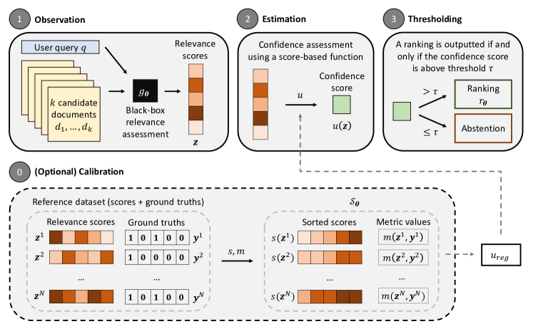
Figure 1: Procedure diagram for black-box confidence estimation and abstention decision in a reranking setting. In the reference-free scenario, confidence function $u$ is a simple heuristic (e.g., maximum). In the reference-based scenario, $u$ is a light non-trivial function of the relevance scores (e.g., learned linear combination).

In this paper, as stated in Section 2.2, the confidence scorer we build only takes into account the vector of relevance scores. The intuition behind such an approach is that it is possible, given the distribution of these scores, to estimate the degree of confidence of our ranker on a given instance. In the next two subsections, we describe two methods to calculate this confidence score: the first being reference-free, and the second one requiring an access to a reference dataset.

3.1 Reference-Free Scenario

First, we present the reference-free approach, which can be divided into three stages (Figure 1).
1. Observation. We first observe the relevance scores $\mathbf{z}=g_{\bm{\theta}}(x)$ (Equation 2) for a given test instance $x=\left(q,d_{1},\cdots,d_{k}\right)\in\mathcal{Q}\times\mathcal{D}^{k}$.
2. Estimation. We then assess confidence using a simple heuristic function $u_{\text{base}}$, based solely on these relevance scores (e.g., maximum).
3. Thresholding. Finally, we compare the confidence score computed in step 2 to a threshold $\tau$. If $u_{\text{base}}(\mathbf{z})>\tau$, we make a prediction using ranker $r_{\bm{\theta}}$, otherwise, we abstain (Equation 5).

In this work, we evaluate a bunch of reference-free confidence functions, relying on simple statistics computed on the vector of relevance scores. We focus more particularly on three functions inspired from MSP Hendrycks and Gimpel (2016): (i) the maximum relevance score $u_{\text{max}}$, (ii) the standard deviation of the relevance scores $u_{\text{std}}$, and (iii) the difference between the first and second highest relevance scores $u_{\text{1-2}}$ Narayanan et al. (2012).

3.2 Data-Driven Scenario

In this scenario, rather than arbitrarily constructing a relevance-score-based confidence scorer, we consider that we have access to a reference set $\mathcal{S}=\left\{(x^{i},\mathbf{y}^{i})\right\}_{i=1}^{N}$ (Equation 1) and are therefore able to evaluate ranker $r_{\bm{\theta}}$ (Equation 4) on each of the $N$ labeled instances. We thus define dataset $\mathcal{S}_{\bm{\theta}}$:

$$\mathcal{S}_{\bm{\theta}}=\left\{\left(s_{\bm{\theta}}(x),m\left(g_{\bm{\theta}}(x),\mathbf{y}\right)\right)\ |\ (x,\mathbf{y})\in\mathcal{S}\right\}.$$ (6)

As a reminder, $s_{\bm{\theta}}(x)$ is the ascending sort of query-document relevance scores (Equation 3) and $m\left(g_{\bm{\theta}}(x),\mathbf{y}\right)$ is the evaluation of the ranking induced by $g_{\bm{\theta}}(x)$ given ground truth $\mathbf{y}$ and metric function $m$.

An intuitive approach is to fit a simple supervised model whose objective is to predict ranking performance $m\left(g_{\bm{\theta}}(x),\mathbf{y}\right)$ given a vector of sorted relevance scores $s_{\bm{\theta}}(x)$. In this section, we develop a regression-based approach (see Figure 1).
0. Calibration. We use reference set $\mathcal{S}$ to derive $\mathcal{S}_{\bm{\theta}}$ (Equation 6) and then fit a regressor $h_{\text{reg}}:\mathbb{R}^{k}\rightarrow\mathbb{R}$ on $\mathcal{S}_{\bm{\theta}}$. Next, we derive $u_{\text{reg}}=h_{\text{reg}}\circ s$, the function that takes a vector of unsorted scores as input and returns the predicted ranking quality.
1. Observation. As in 3.1, we observe the relevance scores $\mathbf{z}=g_{\bm{\theta}}(x)$ for a given test instance $x$.
2. Estimation. We then assess confidence using the $u_{\text{reg}}$ function. Intuitively, the greater $u_{\text{reg}}(\mathbf{z})$, the more confident we are that $r_{\bm{\theta}}$ correctly ranks the documents with respect to the query.
3. Thresholding. As in 3.1, an abstention decision is finally made by comparing $u_{\text{reg}}(\mathbf{z})$ to $\tau$. In Section 5.3, we propose an approach to choose $\tau$.

In this work, we use a linear-regression-based confidence function $u_{\text{lin}}$ Fisher (1922). Formally, for a given unsorted vector of relevance scores $\mathbf{z}$,

$$u_{\text{lin}}(\mathbf{z})=\beta_{0}+\beta_{1}s_{1}(\mathbf{z})+\cdots+\beta_{k}s_{k}(\mathbf{z}),$$

where $\beta_{0},\cdots,\beta_{k}\in\mathbb{R}$ are the coefficients fitted on $\mathcal{S}_{\bm{\theta}}$, with an $l_{2}$ regularization parameter $\lambda=0.1$ Hoerl and Kennard (1970). More data-driven confidence functions are explored in Appendix D.

4 Experimental Setup

In this section, we propose a novel experimental setup for assessing the performance of abstention mechanisms in a black-box reranking setting. We present the datasets and models that make up our benchmark, as well as the evaluation methods used.

4.1 Models and Datasets

An extensive benchmark is built to evaluate the abstention mechanisms presented in Section 3. We collect six open-source reranking datasets Lhoest et al. (2021) in three different languages, English, French and Chinese: stackoverflowdupquestions-reranking Zhang et al. (2015), denoted StackOverflow in the experiments, askubuntudupquestions-reranking Lei et al. (2015), denoted AskUbuntu, scidocs-reranking Cohan et al. (2020), denoted SciDocs, mteb-fr-reranking-alloprof-s2p Lefebvre-Brossard et al. (2023), denoted Alloprof, CMedQAv1-reranking Zhang et al. (2017), denoted CMedQAv1, and Mmarco-reranking Bonifacio et al. (2021), denoted Mmarco.

We also collect 22 open-source models for evaluation on each of the six datasets. These include models of various sizes, bi-encoders and cross-encoders, monolingual and multilingual: ember-v1 (paper to be released soon), llm-embedder Zhang et al. (2023), bge-base-en-v1.5, bge-reranker-base/large Xiao et al. (2023), multilingual-e5-small/large, e5-small-v2/large Wang et al. (2022), msmarco-MiniLM-L6-cos-v5, msmarco-distilbert-dot-v5, ms-marco-TinyBERT-L-2-v2, ms-marco-MiniLM-L-6-v2 Reimers and Gurevych (2021), stsb-TinyBERT-L-4, stsb-distilroberta-base, multi-qa-distilbert-cos-v1, multi-qa-MiniLM-L6-cos-v1, all-MiniLM-L6-v2, all-distilroberta-v1, all-mpnet-base-v2, quora-distilroberta-base and qnli-distilroberta-base Reimers and Gurevych (2019).

In addition, each dataset is preprocessed in such a way that there are only 10 candidate documents per query and a maximum of five positive documents, in order to create a scenario close to real-life reranking use cases. Moreover, to fit the black-box setting, query-documents relevance scores are calculated upstream of the evaluation and are not used thereafter. Further details are given in appendix A.

4.2 Instance-Wise Metrics

In this work, we rely on three of the metrics most commonly used in the IR setting (e.g., in the MTEB leaderboard Muennighoff et al. (2022)): Average Precision (AP), Normalized Discounted Cumulative Gain (NDCG) and Reciprocal Rank (RR): AP Zhu (2004) computes a proxy of the area under the precision-recall curve; NDCG Järvelin and Kekäläinen (2002) measures the relevance of the top-ranked items by discounting those further down the list using a logarithmic factor; and RR Voorhees et al. (1999) computes the inverse rank of the first relevant element in the predicted ranking. For all three metrics, higher values indicate better performance. Note that, when relevant, we rely on their averaged versions across multiple instances: mAP, mNDCG and mRR.

4.3 Assessing Abstention Performance

The compromise between abstention rate and performance in predictive modeling represents a delicate balance that requires careful consideration El-Yaniv and Wiener (2010). First, we want to make sure that an increasing abstention rate implies increasing performance, otherwise the mechanism employed is ineffective or even deleterious. Secondly, we aim to abstain in the best possible way for every abstention rate, i.e., we want to maximize the growth of the performance-abstention curve.

Inspired by the risk-coverage curve El-Yaniv and Wiener (2010); Geifman and El-Yaniv (2017), we evaluate abstention strategies by reporting the normalized Area Under the performance-abstention Curve, where the x-axis corresponds to the abstention rate of the strategy and the y-axis to the achieved average performance regarding metric function $m$. Our evaluation protocol can be divided into four steps, assuming access to a test set, $\mathcal{S}^{\prime}$.
1. Multi-thresholding. First of all, we evaluate abstention mechanism $\rho_{\bm{\theta}}$ (Equation 5) on test set $\mathcal{S}^{\prime}$ for a list of abstention thresholds $\tau_{1}<...<\tau_{n}\in\mathbb{R}$. For a given $\tau\in\mathbb{R}$, the performance of mechanism $\rho_{\bm{\theta}}$ on $\mathcal{S}^{\prime}$ and its corresponding abstention rate are respectively denoted by

$$\begin{cases}\begin{aligned} P_{\tau,m}\left(\rho_{\bm{\theta}}\right)&=\frac{1}{\left|\mathcal{S}_{\tau}^{\prime}\right|}\sum_{\left(x,\mathbf{y}\right)\in\mathcal{S}_{\tau}^{\prime}}m\left(r_{\bm{\theta}}(x),\mathbf{y}\right),\\ R_{\tau}\left(\rho_{\bm{\theta}}\right)&=1-\frac{\left|\mathcal{S}_{\tau}^{\prime}\right|}{\left|\mathcal{S}^{\prime}\right|}\end{aligned}\end{cases},$$ (7)

$\mathcal{S}_{\tau}^{\prime}$ being the set of predicted instances, i.e., $\mathcal{S}_{\tau}^{\prime}=\left\{\left(x,\mathbf{y}\right)\in\mathcal{S}^{\prime}\ |\ \rho_{\bm{\theta}}\left(x,\tau\right)\neq\perp\right\}$. We collect $n$ abstention rates, $\left(R_{\tau_{i}}\left(\rho_{\bm{\theta}}\right)\right)_{i=1}^{n}$, and associated performances, $\left(P_{\tau_{i},m}\left(\rho_{\bm{\theta}}\right)\right)_{i=1}^{n}$, and compute the area under the curve $AUC_{m}\left(\rho_{\bm{\theta}}\right)$ for metric function $m$.
2. Random mechanism evaluation. Second, we evaluate $\tilde{\rho}$, the mechanism that performs random (i.e., ineffective) abstention. Intuitively, random abstention shows flat performance as the abstention rate increases, equal to $P_{-\infty,m}\left(\rho_{\bm{\theta}}\right)$ (Equation 7).
3. Oracle evaluation. Then, we evaluate the oracle $\rho^{*}$ on the same task. Intuitively, the oracle has access to the test labels and can therefore select the best instances for a given abstention rate. $AUC_{m}\left(\rho^{*}\right)$ thus upper-bounds $AUC_{m}\left(\rho_{\bm{\theta}}\right)$.
4. Normalization. We finally compute normalized AUC. Formally,

$$nAUC_{m}\left(\rho_{\bm{\theta}}\right)=\frac{AUC_{m}\left(\rho_{\bm{\theta}}\right)-AUC_{m}\left(\tilde{\rho}\right)}{AUC_{m}\left(\rho^{*}\right)-AUC_{m}\left(\tilde{\rho}\right)}.$$ (8)

In particular, $nAUC_{m}(\rho_{\bm{\theta}})=1$ means that abstention mechanism $\rho_{\bm{\theta}}$ reaches oracle performance. In contrast, $nAUC_{m}(\rho_{\bm{\theta}})<0$ indicates that $\rho_{\bm{\theta}}$ has a deleterious effect, with declining average ranking performance while abstention increases.

In this study, in order to guarantee consistent comparisons between abstention mechanisms, we randomly set aside 20% of the initial dataset as a test set, treating the remaining 80% as the reference set. Results, unless specified otherwise, are averaged across five random seeds.

5 Results

5.1 Abstention Performance

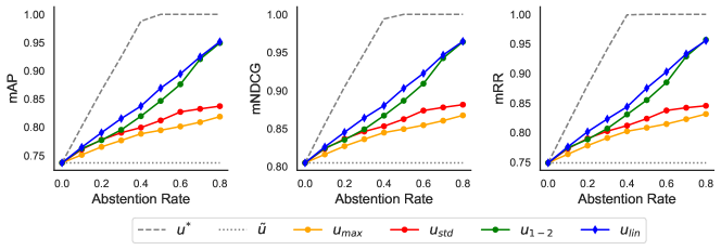
Figure 2: Performance-abstention curves for the ember-v1 model on the StackOverflow dataset. All methods show increasing curves, indicating effective abstention. The reference-based method, $u_{\text{lin}}$, stands out above the others, demonstrating superior abstention performance. Note that $u^{*}$ and $\tilde{u}$ respectively denote the oracle and the random abstention confidence functions.

Table 1: Abstention performance assessment. nAUCs (in %) averaged model-wise, for each method, dataset and metric.

	Method	$u_{\text{max}}$	$u_{\text{std}}$	$u_{\text{1-2}}$	$u_{\text{lin}}$
Dataset	Metric
SciDocs	mAP	49.2	58.7	4.7	65.4
	mNDCG	54.9	62.9	10.2	66.6
	mRR	80.2	80.3	41.3	80.5
AskUbuntu	mAP	24.1	16.2	7.3	22.0
	mNDCG	28.1	15.7	8.6	24.5
	mRR	32.7	16.6	14.0	26.2
StackOverflow	mAP	20.7	24.6	35.7	42.6
	mNDCG	21.0	25.0	35.6	42.6
	mRR	21.4	24.8	36.1	42.8
Alloprof	mAP	16.6	17.0	19.3	29.7
	mNDCG	16.8	16.9	18.8	29.3
	mRR	16.9	16.7	19.1	28.9
CMedQAv1	mAP	24.4	23.3	22.3	30.6
	mNDCG	25.0	23.5	22.3	30.7
	mRR	26.5	24.2	23.4	31.5
Mmarco	mAP	30.1	31.0	39.4	34.0
	mNDCG	30.5	30.9	38.8	34.1
	mRR	30.1	31.0	39.6	34.3
Average	mAP	27.5	28.5	21.5	37.4
	mNDCG	29.4	29.1	22.4	38.0
	mRR	34.6	32.3	28.9	40.7

We report abstention nAUC (Equation 8) for all methods described in Section 3, averaged model-wise (Table 1), and illustrate the dynamics of the performance-abstention curves for the ember-v1 model on the StackOverflow dataset in Figure 2.

Abstention works. All evaluated abstention-based methods improve downstream evaluation metrics (nAUCs greater than 0), showcasing the relevance of abstention approaches in a practical setting.

Reference-based abstention works better. The value of reference-based abstention approaches is demonstrated in Table 1, in which we notice that the linear-regression-based method $u_{\text{lin}}$ performs on average largely better than all reference-free baselines, edging out the best baseline strategy ($u_{\text{std}}$) by almost 10 points on the mAP metric.

Having shown the superiority of reference-based abstention methods across the entire benchmark, we conduct (unless otherwise specified) the following experiments on the ember-v1 model using the mAP as a metric function, and compare $u_{\text{lin}}$ to $u_{\text{std}}$, the best reference-free method mAP-wise.

5.2 Abstention Effectiveness vs. Raw Model Performance

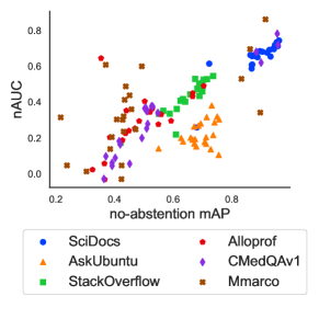
Figure 3: Abstention performance (nAUC in %) vs. no-abstention performance (mAP), for all models and datasets, using $u_{\text{lin}}$ as a confidence function. Each data point represents a model-dataset pair.

Table 2: Pearson’s correlations between no-abstention mAP and abstention nAUC, for each dataset.

Dataset	Correlation
SciDocs	0.85
AskUbuntu	0.38
StackOverflow	0.90
Alloprof	0.56
CMedQAv1	0.94
Mmarco	0.63
General	0.73

We investigate whether a correlation exists between abstention effectiveness and model raw performance (i.e., without abstention) on the reranking task. For each model-dataset pair, we compute both no-abstention mAP and abstention nAUC, using $u_{\text{lin}}$ as a confidence function (Figure 3, Table 2).

A better ranker implies better abstention. Figure 3 and Table 2 showcase a clear positive correlation between model raw performance and abstention effectiveness, albeit with disparities from one dataset to another. Logically, better reranking methods exhibit more calibrated score distributions, enabling better abstention performance. This finding reinforces the interest of implementing abstention mechanisms in high-performance retrieval systems.

5.3 Threshold Calibration

Table 3: Threshold calibration analysis. MAEs between target and achieved abstention rates and performance levels (in %) (model: ember-v1, dataset: StackOverflow, metric: mAP).

	Target Abstention	10%	50%	90%
Rate	$u_{\text{std}}$	1.10	1.80	1.08
	$u_{\text{lin}}$	1.07	1.79	1.09
mAP	$u_{\text{std}}$	1.24	1.52	3.09
	$u_{\text{lin}}$	1.22	1.33	1.51

In practical industrial settings, a major challenge with abstention methods lies in choosing the right threshold to ensure a desired abstention rate or performance level on new data. To evaluate threshold calibration quality, we sequentially choose three target abstention rates (10%, 50%, and 90%) and rely on the reference set to infer the corresponding threshold and level of performance (here, the mAP). Then, the Mean Absolute Error (MAE) between target and achieved values on test instances is reported (Table 3), averaging across 1000 random seeds on the StackOverflow dataset.

$u_{\text{lin}}$ is better calibrated than $u_{\text{std}}$. The lower part of Table 3 shows that the MAE between the target and achieved mAP increases with the abstention rate, which is logical because a higher abstention rate reduces the number of evaluated instances and therefore increases volatility. However, we observe that the MAE increases much less significantly for the $u_{\text{lin}}$ method than for the $u_{\text{std}}$ method, with the latter having a MAE twice as high at a target abstention rate of 90%. This provides strong evidence that $u_{\text{lin}}$ is more reliable at high abstention rates.

5.4 Domain Adaptation Study

Table 4: Domain adaptation study. nAUCs (in %) averaged test-set-wise (model: ember-v1, metric: mAP).

Method	$u_{\text{max}}$	$u_{\text{std}}$	$u_{\text{1-2}}$	$u_{\text{lin}}$
Reference set
Alloprof	30.1	32.7	17.1	31.4
AskUbuntu	28.5	32.1	19.8	34.2
CMedQAv1	27.9	31.1	17.2	34.2
Mmarco	27.5	32.2	18.9	34.9
SciDocs	23.0	23.5	22.3	11.6
StackOverflow	29.3	30.7	11.9	20.6
Average	27.7	30.4	17.9	27.8

In a practical setting, it is rare to have a reference set that perfectly matches the distribution of samples seen at test time. To measure the robustness of our method to strong data drifts, we fit them on a given dataset and evaluate on all others.

Reference-based approaches are globally not robust to domain changes. From Table 4, we see on average that the reference-based method underperforms reference-free baselines when fitted on the "wrong" reference set. However, certain reference datasets seem to enable methods to generalize better overall, even out of distribution, which is mainly an artifact of the number of positive documents per instance (further insights in Appendix C).

5.5 Reference Set Minimal Size

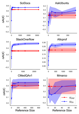
Figure 4: Reference set size analysis. nAUC vs. reference set size for $u_{\text{lin}}$ and $u_{\text{std}}$ on all datasets (model: ember-v1, metric: mAP).

Table 5: Reference set size analysis. Minimum reference set size required for $u_{\text{lin}}$ to outperform $u_{\text{std}}$ (model: ember-v1, metric: mAP).

Dataset	Break-Even
SciDocs	12
AskUbuntu	9
StackOverflow	19
Alloprof	58
CMedQAv1	50
Mmarco	80
Average	38

Calibrated reference-based methods outperform reference-free baselines (Section 5.1) but require having access to an in-domain reference set (Section 5.4). To assess the efforts required for calibrating these techniques to extract best abstention performance, we study the impact of reference set size on method performance.

Small reference sets suffice. From Figure 4 and Table 5, we note that $u_{\text{lin}}$ requires only a fairly small amount of reference data (less than 40 samples on average) to outperform $u_{\text{std}}$, which demonstrates the effectiveness of using a reference set even when data is scarce. This demonstrates the applicability of our method to practical industrial contexts, the labeling of around 50 samples appearing perfectly tractable in such settings.

5.6 Computational Overhead Analysis

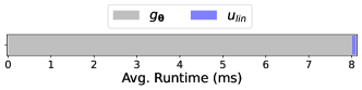
Figure 5: Computational overhead analysis. Comparison between relevance score ($g_{\bm{\theta}}$) and confidence score ($u_{\text{lin}}$) calculation times (on average, 8 ms and 0.1 ms respectively on one Apple M1 CPU) (model: all-MiniLM-L6-v2, dataset: StackOverflow).

Crucial to the adoption of our abstention method is the minor latency overhead incurred at inference time. In our setup, we consider documents are pre-embedded by the bi-encoders, and stored in a vector database. We average timed results over 100 runs on a single instance prediction, running the calculations on one Apple M1 CPU (Figure 5). To upper-bound the abstention method overhead, we baseline the smallest model with the fastest embedding time available (all-MiniLM-L6-v2).

Our data-based abstention method is free of any significant time overhead. $u_{\text{lin}}$-based confidence estimation accounts for only 1.2% of the time needed for relevance scores computation (Figure 5), making it an almost cost-free option.

6 Conclusion

We developed a lightweight abstention mechanism tailored to real-world constraints, agnostic to the ranking method and shown to be effective across various settings and use cases. Our method, which only requires black-box access to relevance scores and a small reference set for calibration, is essentially a free-lunch to plug to any retrieval system, in order to gain better control over the whole IR pipeline. A logical next step would be to generalize findings to ensembling-based retrieval methods which boost downstream performance while outputting a richer signal for confidence estimations.

Limitations

Our work studies abstention mechanisms within the scope of the reranking stage of a larger information retrieval pipeline. While this enables estimating confidence for the final prediction of the IR system, the lack of existing document-wise-labeled datasets has prevented us from evaluating our methods at the primary ranking stage, although they should theoretically be directly applicable. Additionally, our study primarily focuses on reranking scenarios with the top-10 retrieved documents, which correspond to standard industrial use cases, but it would be interesting to extend this scenario to top-50 or top-100 documents. Our linear-regression-based abstention method is easily scalable and should theoretically benefit from additional document scores in its decision-making process, but the performance impact remains to be quantified. Finally, in RAG applications, an LLM is given the retrieved documents as context, but might not use all of them to formulate an answer, thus acting as a final abstention mechanism. Studies have even shown these RAG LLMs work best when given a certain ratio of non-relevant documents in order to induce a filtering behavior Cuconasu et al. (2024). Studying the impact of abstention mechanisms on end-to-end RAG performance would thus be an interesting future work direction. Additionally, in the future, we could rely on anomaly detection algorithms to remove any need for training, specifically, we want to investigate the use of isolation forest Darrin et al. (2023), data depths Colombo et al. (2022, 2023b); Staerman et al. (2021); Picot et al. (2022a, b), information measures Colombo et al. (2023a) and projections Darrin et al. (2022); Picot et al. (2022c), and Wasserstein distances Guerreiro et al. (2022).

Ethical Statement

The proposed abstention mechanism enables IR systems to refrain from making predictions when signs of unreliability are detected. This approach enhances the accuracy and effectiveness of retrieval systems, but also contributes to the construction of a more trustworthy AI technology, by reducing the risks of providing potentially inaccurate or irrelevant results to users. Furthermore, abstention enables downstream systems to avoid using computational resources on unreliable or irrelevant predictions, optimizing resource utilization and therefore minimizing energy consumption. In the context of RAG systems, where large-scale computations are prevalent, introducing abstention mechanisms is a positive stride towards trustworthy and sustainable AI development, reducing overall computational demands while potentially improving system performance.

Appendices

Appendix A Additional Information on Models and Datasets

Table 6: Dataset details after preprocessing.

	$N$	$k$	$p_{\text{min}}$	$p_{\text{max}}$	$\bar{p}$
SciDocs	3978	10	1	5	4.9
AskUbuntu	351	10	1	5	3.6
StackOverflow	2980	10	1	5	1.2
Alloprof	2316	10	1	5	1.3
CMedQAv1	1000	10	1	5	1.8
Mmarco	100	10	1	3	1.1

Table 7: Details on raw datasets.

	Reference	Language	$N$	$k_{\text{min}}$	$k_{\text{max}}$	$\bar{k}$	$p_{\text{min}}$	$p_{\text{max}}$	$\bar{p}$
SciDocs	Cohan et al. 2020	English	3978	26	60	29.8	1	10	4.9
AskUbuntu	Lei et al. 2015	English	375	20	20	20.0	1	20	6.0
StackOverflow	Zhang et al. 2015	English	2992	20	30	29.9	1	6	1.2
Alloprof	Lefebvre-Brossard et al. 2023	French	2316	10	35	10.7	1	29	1.3
CMedQAv1	Zhang et al. 2017	Chinese	1000	100	100	100.0	1	19	1.9
Mmarco	Bonifacio et al. 2021	Chinese	100	1000	1002	1000.3	1	3	1.1

Table 8: Model details.

	Reference	Languages	Type	Similarity	$|\bm{\theta}|$
ember-v1	TBA	English	bi	cos	335
llm-embedder	Zhang et al. 2023	English	bi	cos	109
bge-base-en-v1.5	Xiao et al. 2023	English	bi	cos	109
bge-reranker-base	Xiao et al. 2023	English, Chinese	cross	n.a.	278
bge-reranker-large	Xiao et al. 2023	English, Chinese	cross	n.a.	560
e5-small-v2	Wang et al. 2022	English	bi	cos	33
e5-large-v2	Wang et al. 2022	English	bi	cos	335
multilingual-e5-small	Wang et al. 2022	94	bi	cos	118
multilingual-e5-large	Wang et al. 2022	94	bi	cos	560
msmarco-MiniLM-L6-cos-v5	Reimers and Gurevych 2021	English	bi	cos	23
msmarco-distilbert-dot-v5	Reimers and Gurevych 2021	English	bi	cos	66
ms-marco-TinyBERT-L-2-v2	Reimers and Gurevych 2021	English	cross	n.a.	4
ms-marco-MiniLM-L-6-v2	Reimers and Gurevych 2021	English	cross	n.a.	23
stsb-TinyBERT-L-4	Reimers and Gurevych 2019	English	cross	n.a.	14
stsb-distilroberta-base	Reimers and Gurevych 2019	English	cross	n.a.	82
multi-qa-distilbert-cos-v1	Reimers and Gurevych 2019	English	bi	cos	66
multi-qa-MiniLM-L6-cos-v1	Reimers and Gurevych 2019	English	bi	cos	23
all-MiniLM-L6-v2	Reimers and Gurevych 2019	English	bi	cos	23
all-distilroberta-v1	Reimers and Gurevych 2019	English	bi	cos	82
all-mpnet-base-v2	Reimers and Gurevych 2019	English	bi	cos	109
quora-distilroberta-base	Reimers and Gurevych 2019	English	cross	n.a.	82
qnli-distilroberta-base	Reimers and Gurevych 2019	English	cross	n.a.	82

Table 9: Models’ raw performances (mAP, mNDCG, mRR without abstention) on the whole benchmark.

Dataset $\rightarrow$	SciDocs			AskUbuntu			StackOverflow			Alloprof			CMedQAv1			Mmarco			Average
Metric $\rightarrow$	mAP	mNDCG	mRR	mAP	mNDCG	mRR	mAP	mNDCG	mRR	mAP	mNDCG	mRR	mAP	mNDCG	mRR	mAP	mNDCG	mRR	mAP	mNDCG	mRR
Model $\downarrow$
ember-v1	0.96	0.98	0.99	0.74	0.85	0.84	0.74	0.81	0.75	0.55	0.66	0.56	0.51	0.64	0.55	0.43	0.57	0.44	0.65	0.75	0.69
llm-embedder	0.94	0.97	0.99	0.71	0.83	0.82	0.70	0.78	0.72	0.52	0.64	0.53	0.51	0.64	0.55	0.47	0.60	0.47	0.64	0.74	0.68
bge-base-en-v1.5	0.93	0.97	0.98	0.73	0.84	0.83	0.72	0.79	0.73	0.53	0.65	0.54	0.53	0.66	0.57	0.45	0.58	0.45	0.65	0.75	0.68
bge-reranker-base	0.87	0.94	0.96	0.67	0.80	0.78	0.57	0.68	0.58	0.67	0.75	0.68	0.96	0.97	0.96	0.90	0.92	0.90	0.77	0.84	0.81
bge-reranker-large	0.88	0.95	0.97	0.71	0.82	0.81	0.59	0.69	0.60	0.70	0.78	0.72	0.96	0.97	0.96	0.92	0.94	0.92	0.79	0.86	0.83
e5-small-v2	0.93	0.97	0.98	0.69	0.81	0.78	0.68	0.76	0.70	0.48	0.61	0.50	0.53	0.66	0.57	0.44	0.57	0.44	0.63	0.73	0.66
e5-large-v2	0.95	0.98	0.99	0.71	0.83	0.81	0.69	0.77	0.70	0.56	0.67	0.57	0.55	0.67	0.59	0.49	0.61	0.50	0.66	0.76	0.69
multilingual-e5-small	0.92	0.96	0.98	0.69	0.82	0.80	0.68	0.76	0.69	0.59	0.70	0.61	0.88	0.92	0.90	0.83	0.87	0.83	0.77	0.84	0.80
multilingual-e5-large	0.94	0.98	0.99	0.71	0.83	0.81	0.69	0.77	0.70	0.67	0.75	0.68	0.90	0.93	0.92	0.86	0.90	0.86	0.80	0.86	0.83
msmarco-MiniLM-L6-cos-v5	0.86	0.94	0.96	0.67	0.80	0.79	0.62	0.72	0.64	0.38	0.53	0.40	0.42	0.57	0.45	0.37	0.52	0.37	0.56	0.68	0.60
msmarco-distilbert-dot-v5	0.87	0.94	0.97	0.68	0.81	0.79	0.64	0.73	0.65	0.44	0.58	0.45	0.45	0.60	0.49	0.43	0.57	0.44	0.59	0.70	0.63
ms-marco-TinyBERT-L-2-v2	0.87	0.94	0.96	0.63	0.77	0.74	0.63	0.73	0.65	0.45	0.58	0.46	0.40	0.56	0.43	0.41	0.55	0.41	0.57	0.69	0.61
ms-marco-MiniLM-L-6-v2	0.89	0.95	0.97	0.66	0.79	0.75	0.66	0.75	0.67	0.52	0.64	0.53	0.42	0.57	0.45	0.43	0.56	0.43	0.60	0.71	0.63
stsb-TinyBERT-L-4	0.87	0.94	0.96	0.63	0.77	0.73	0.55	0.66	0.56	0.33	0.49	0.33	0.39	0.55	0.42	0.39	0.53	0.39	0.53	0.66	0.57
stsb-distilroberta-base	0.87	0.94	0.96	0.67	0.80	0.79	0.61	0.71	0.63	0.43	0.57	0.44	0.37	0.54	0.40	0.22	0.40	0.21	0.53	0.66	0.57
multi-qa-distilbert-cos-v1	0.90	0.96	0.97	0.75	0.85	0.84	0.70	0.78	0.71	0.51	0.63	0.53	0.51	0.64	0.55	0.39	0.53	0.39	0.63	0.73	0.66
multi-qa-MiniLM-L6-cos-v1	0.90	0.95	0.97	0.73	0.84	0.82	0.68	0.76	0.69	0.44	0.58	0.45	0.51	0.65	0.55	0.42	0.56	0.42	0.61	0.72	0.65
all-MiniLM-L6-v2	0.95	0.98	0.99	0.74	0.84	0.83	0.69	0.77	0.70	0.35	0.50	0.36	0.50	0.64	0.55	0.46	0.59	0.46	0.62	0.72	0.65
all-distilroberta-v1	0.96	0.98	0.99	0.76	0.85	0.85	0.70	0.78	0.71	0.47	0.60	0.49	0.49	0.63	0.54	0.43	0.57	0.44	0.63	0.74	0.67
all-mpnet-base-v2	0.96	0.98	0.99	0.76	0.85	0.85	0.70	0.78	0.71	0.50	0.63	0.52	0.51	0.65	0.55	0.42	0.56	0.42	0.64	0.74	0.67
quora-distilroberta-base	0.72	0.86	0.89	0.67	0.80	0.79	0.61	0.71	0.62	0.37	0.52	0.38	0.39	0.55	0.43	0.24	0.41	0.24	0.50	0.64	0.56
qnli-distilroberta-base	0.68	0.82	0.80	0.55	0.71	0.63	0.42	0.56	0.43	0.37	0.52	0.38	0.36	0.53	0.40	0.30	0.46	0.30	0.45	0.60	0.49

In this section, we give details on the datasets used in our work, before the preprocessing phase (Table 7), and after preprocessing (Table 6). As in the main text, $N$ denotes the number of instances and $k$ represents the number of candidate documents. In the same logic, $k_{\text{min}}$, $k_{\text{max}}$ and $\bar{k}$ respectively denote the minimum, maximum and average number of candidate documents in the dataset. In addition, $p_{\text{min}}$, $p_{\text{max}}$, $\bar{p}$ denote the minimum, maximum and average number of positive documents respectively. Additionally, we provide information on models’ raw performance (without abstention) across the whole benchmark in Table 9.

In the data preprocessing phase, we limit the number of candidate documents to 10 and the number of positive documents per instance to five, for the sake of realism and simplicity. Intuitively, these 10 documents are to be interpreted as the output of a retriever. In practice, for each instance taken from a raw dataset, we randomly sample the positive documents (maximum of five) and complete with a random sampling of the negative documents. When a raw instance contains fewer than 10 documents, it is automatically discarded.

Additionally, we provide some details about the 22 models used in our study (Table 8): their reference paper, the language(s) in which they were trained, their type (bi-encoder or cross-encoder), the similarity function used (when applicable) and finally their number of parameters denoted $|\bm{\theta}|$ (in millions).

Appendix B Additional Results on Abstention Performance

Table 10: Methods’ nAUCs (in %) on the whole benchmark.

	Dataset $\rightarrow$	SciDocs				AskUbuntu				StackOverflow				Alloprof				CMedQAv1				Mmarco
	Method $\rightarrow$	$u_{\text{max}}$	$u_{\text{std}}$	$u_{\text{1-2}}$	$u_{\text{lin}}$	$u_{\text{max}}$	$u_{\text{std}}$	$u_{\text{1-2}}$	$u_{\text{lin}}$	$u_{\text{max}}$	$u_{\text{std}}$	$u_{\text{1-2}}$	$u_{\text{lin}}$	$u_{\text{max}}$	$u_{\text{std}}$	$u_{\text{1-2}}$	$u_{\text{lin}}$	$u_{\text{max}}$	$u_{\text{std}}$	$u_{\text{1-2}}$	$u_{\text{lin}}$	$u_{\text{max}}$	$u_{\text{std}}$	$u_{\text{1-2}}$	$u_{\text{lin}}$
Model $\downarrow$	Metric $\downarrow$
all-MiniLM-L6-v2	mAP	-6.3	73.4	52.5	66.5	6.0	21.6	23.6	13.5	35.6	43.5	19.0	25.1	28.3	64.5	37.1	-8.3	30.5	36.5	28.6	25.0	27.6	36.0	23.2	11.2
	mNDCG	-2.2	74.9	59.7	71.8	6.7	24.3	29.4	13.5	35.5	43.4	19.3	25.7	27.2	63.1	37.3	-7.0	29.6	36.6	28.6	24.1	27.6	36.1	24.5	11.3
	mRR	24.0	91.3	89.8	93.3	13.9	32.5	38.8	21.6	36.5	43.6	20.3	25.6	28.4	61.9	37.9	-7.4	27.9	36.0	28.8	24.1	29.6	37.8	23.3	10.3
all-distilroberta-v1	mAP	-5.8	71.3	49.9	63.3	25.2	10.5	26.1	9.0	41.7	47.1	16.5	24.4	17.2	25.3	20.1	17.6	15.5	20.0	3.5	12.4	25.9	23.5	19.7	18.0
	mNDCG	-0.5	72.0	56.5	67.7	26.5	16.3	31.9	8.3	41.6	47.3	16.7	25.0	16.8	25.0	19.9	17.2	15.4	18.8	4.9	12.4	24.9	21.0	19.8	17.3
	mRR	36.8	91.1	93.7	89.1	32.9	24.1	42.2	12.2	42.1	47.4	17.1	24.7	17.0	24.1	19.2	16.9	15.5	18.5	7.9	13.0	26.7	25.2	19.0	18.3
all-mpnet-base-v2	mAP	-11.4	74.4	51.0	64.9	19.2	30.3	34.6	19.7	43.4	50.6	20.0	24.1	28.4	40.4	27.2	22.2	19.5	27.8	19.3	22.2	18.9	4.7	7.6	18.8
	mNDCG	-9.8	75.7	57.0	69.7	22.5	33.7	39.1	17.9	43.4	50.4	20.7	24.8	27.7	40.0	27.6	22.2	18.5	25.7	18.7	21.4	18.7	6.3	8.6	19.8
	mRR	10.9	90.2	89.0	93.6	31.5	37.0	45.1	19.1	44.0	50.6	21.6	24.5	28.3	40.4	27.8	22.0	18.4	24.6	19.1	21.3	20.2	7.7	8.2	19.5
bge-base-en-v1.5	mAP	-1.4	65.4	46.4	58.2	0.7	38.1	35.2	14.2	46.4	52.8	23.9	32.3	27.8	36.4	17.1	25.0	24.4	37.7	29.1	34.4	38.2	43.8	40.0	27.7
	mNDCG	4.7	66.5	53.3	62.1	0.5	38.8	39.2	10.2	46.1	53.1	24.5	32.8	26.8	35.3	17.2	24.8	23.2	36.6	28.8	34.2	36.2	45.2	40.5	27.0
	mRR	40.4	83.1	83.7	79.8	3.8	37.6	41.7	3.1	46.4	52.6	24.8	32.5	26.6	34.9	16.6	24.4	23.8	36.2	28.6	34.1	38.5	43.3	39.6	26.6
bge-reranker-base	mAP	2.7	58.7	47.1	53.8	-8.9	19.0	24.2	8.1	26.7	35.2	20.7	24.1	38.2	45.0	25.1	30.4	65.1	78.2	74.9	61.4	65.8	34.2	51.3	38.1
	mNDCG	8.5	59.2	51.3	57.0	-6.7	21.1	29.4	7.7	26.6	34.9	20.7	24.4	37.7	44.3	25.4	30.8	67.3	79.7	78.1	64.3	64.4	37.3	53.1	40.5
	mRR	36.4	66.9	67.0	68.1	0.4	22.9	37.5	13.0	27.5	35.9	20.8	24.3	38.0	44.0	25.3	30.7	70.9	83.6	82.3	67.5	64.6	35.3	53.5	42.3
bge-reranker-large	mAP	12.0	65.5	54.2	59.6	-1.7	17.7	23.7	24.4	24.4	33.6	17.1	24.0	44.0	49.0	25.5	32.6	59.6	71.9	70.9	56.9	85.2	86.2	75.8	75.1
	mNDCG	18.0	66.9	59.3	64.0	-1.5	15.5	25.3	23.9	24.2	33.6	17.0	24.1	43.6	48.8	25.9	32.9	61.3	75.8	74.5	59.6	85.3	86.4	76.3	75.5
	mRR	49.1	79.9	80.4	81.4	4.9	6.1	26.5	24.8	24.6	33.9	17.3	24.2	44.0	48.8	26.0	32.5	64.6	78.5	81.0	64.6	85.2	86.2	75.8	75.1
e5-large-v2	mAP	3.2	71.9	52.0	63.7	12.9	20.4	17.6	16.2	39.2	47.2	23.3	27.6	20.6	33.1	18.3	23.9	22.7	34.0	26.8	30.2	64.2	60.0	52.6	54.0
	mNDCG	8.0	72.9	58.1	68.0	16.5	23.9	22.9	15.7	39.1	47.5	23.6	28.1	19.8	32.6	18.4	23.5	22.6	33.4	26.3	29.7	64.0	60.2	53.0	54.2
	mRR	41.6	85.8	87.6	88.2	27.1	24.4	27.1	14.1	40.1	48.1	23.9	28.1	19.8	32.3	18.7	22.9	23.9	32.2	24.7	28.2	64.4	59.4	52.4	53.7
e5-small-v2	mAP	1.1	69.2	49.1	61.8	16.6	26.9	23.1	15.8	38.3	47.5	22.4	27.4	20.5	29.4	12.2	17.9	19.9	37.5	30.8	32.9	50.2	48.8	46.7	47.3
	mNDCG	7.3	70.7	56.1	66.9	18.7	29.2	26.8	14.3	38.3	47.5	22.8	28.0	20.0	29.0	12.7	17.9	20.3	37.4	30.5	32.9	49.1	46.3	46.3	46.7
	mRR	44.2	87.3	86.6	88.3	26.5	29.4	27.6	10.6	38.8	48.1	23.4	27.7	19.8	28.7	13.5	17.4	22.0	37.4	30.8	32.9	50.9	48.5	46.4	46.9
ember-v1	mAP	-4.7	73.6	50.7	65.2	10.2	28.6	30.2	16.3	48.0	54.6	23.7	31.7	20.8	27.6	16.4	20.4	23.6	35.9	28.2	30.5	37.9	41.3	42.2	36.4
	mNDCG	0.4	73.8	56.8	68.4	14.2	30.8	35.2	13.9	47.8	54.0	24.3	32.3	20.2	27.3	16.9	20.4	22.3	34.3	27.5	29.7	36.8	40.4	41.4	35.8
	mRR	34.6	83.6	83.4	81.1	22.2	31.0	41.1	11.3	48.1	54.0	25.0	32.0	20.8	26.9	17.0	19.8	21.7	33.6	27.2	30.6	36.8	41.5	42.1	36.8
llm-embedder	mAP	1.9	69.9	47.2	62.3	1.7	31.6	31.7	20.7	47.1	52.6	26.0	32.3	22.8	34.5	19.7	22.7	21.5	36.7	22.4	29.8	40.5	24.7	18.0	25.5
	mNDCG	5.8	69.9	52.9	66.4	2.1	34.7	36.7	19.4	47.0	52.7	26.5	32.8	22.5	34.4	20.0	22.6	20.6	36.0	23.0	29.9	40.6	25.5	18.8	25.4
	mRR	36.7	86.4	83.1	85.4	6.4	40.3	42.0	19.8	47.8	53.2	26.8	32.5	23.0	34.5	19.7	22.5	21.6	37.5	25.1	31.4	39.8	25.7	19.0	26.4
ms-marco-MiniLM-L-6-v2	mAP	16.1	65.1	52.6	56.3	5.0	20.1	21.7	24.3	38.3	44.3	18.8	21.3	19.9	34.4	24.7	29.3	13.2	16.4	9.2	4.1	18.7	30.1	-6.8	32.9
	mNDCG	25.1	66.6	58.8	61.9	3.6	23.1	25.9	27.3	38.0	44.4	19.2	21.9	19.4	34.1	24.7	29.0	13.4	16.3	9.2	3.5	17.3	30.8	-4.9	32.4
	mRR	72.4	86.4	87.4	86.9	6.2	20.6	29.5	32.7	38.6	44.6	19.4	21.9	20.2	33.9	25.0	29.1	14.5	16.6	8.1	4.5	19.7	28.1	-7.3	32.4
ms-marco-TinyBERT-L-2-v2	mAP	27.6	60.7	53.6	55.6	0.6	18.0	26.5	27.3	32.2	41.7	24.4	20.0	14.0	24.0	12.1	7.9	-2.3	8.9	5.4	-9.1	29.0	30.3	26.5	45.0
	mNDCG	35.4	62.9	59.2	61.0	-0.3	22.4	29.4	29.0	31.9	41.5	24.5	20.5	13.6	23.8	12.4	7.9	-3.3	8.0	4.7	-8.9	27.4	29.5	26.8	43.5
	mRR	76.1	83.4	85.8	85.4	2.4	21.9	30.3	28.4	32.4	41.7	24.5	20.2	14.1	23.8	12.2	8.0	-2.9	5.5	3.4	-7.5	29.8	31.2	27.2	44.2
msmarco-MiniLM-L6-cos-v5	mAP	1.4	66.3	51.5	59.9	10.1	19.3	19.5	12.0	36.0	40.7	22.1	22.1	15.1	20.3	10.6	10.0	16.9	18.2	11.0	9.9	49.3	60.8	21.9	26.8
	mNDCG	7.6	67.4	57.0	63.1	10.3	22.4	24.3	10.1	36.0	41.0	22.6	22.7	14.1	19.3	10.8	9.8	16.1	17.6	10.5	9.0	48.2	58.1	21.9	26.3
	mRR	40.4	79.7	79.5	74.9	14.9	24.3	28.4	6.6	36.6	41.8	23.4	23.3	14.0	17.8	11.1	9.8	17.0	18.5	10.2	7.8	48.7	59.6	22.1	25.4
msmarco-distilbert-dot-v5	mAP	2.3	66.1	50.3	59.7	2.1	15.2	15.1	13.0	36.4	40.2	20.8	24.3	8.7	22.5	11.4	16.2	6.8	5.5	1.3	8.4	54.6	32.1	-0.1	21.8
	mNDCG	8.0	67.4	55.5	63.3	3.0	17.9	20.1	13.1	36.3	40.1	21.1	24.7	8.4	22.2	11.8	15.6	6.4	5.2	2.1	8.2	53.6	29.8	1.0	20.6
	mRR	41.0	79.5	77.7	76.4	11.1	24.9	26.6	13.7	37.2	40.9	21.2	24.6	8.8	22.1	11.4	15.9	7.5	6.2	3.6	6.1	53.4	28.8	0.2	19.9
multi-qa-MiniLM-L6-cos-v1	mAP	-2.1	68.5	52.7	60.6	13.0	13.7	25.1	6.7	42.0	47.5	19.7	27.1	19.0	35.3	32.4	23.2	19.7	34.9	26.6	30.4	22.1	-3.0	15.3	21.6
	mNDCG	4.6	70.5	59.6	66.1	14.6	16.1	30.7	3.0	41.8	47.5	20.2	27.5	18.4	34.9	32.3	22.8	18.5	34.7	27.1	30.4	22.2	-4.4	15.3	21.1
	mRR	40.4	86.9	88.2	87.6	19.2	23.4	40.2	1.6	42.5	47.8	20.8	27.1	18.8	35.2	33.0	23.3	18.8	35.4	28.5	31.5	22.2	-0.2	15.5	22.4
multi-qa-distilbert-cos-v1	mAP	-1.4	68.1	52.3	60.5	20.7	31.9	32.9	27.7	38.6	45.9	19.4	24.1	21.2	34.6	27.0	24.6	20.4	25.3	12.1	18.3	40.5	20.5	29.0	30.9
	mNDCG	4.3	68.8	58.6	65.2	22.6	32.5	38.0	25.8	38.6	46.0	19.6	24.7	20.7	34.4	27.5	24.7	19.8	25.8	12.7	17.9	39.4	21.8	28.8	30.7
	mRR	35.9	81.9	83.7	82.5	27.1	35.0	46.5	26.0	39.4	46.3	20.1	24.5	20.4	34.0	27.6	25.1	21.5	27.8	14.6	18.0	40.6	20.0	29.0	30.5
multilingual-e5-large	mAP	2.8	69.5	49.4	62.6	-16.2	16.8	17.2	10.5	43.2	50.2	23.0	27.5	37.5	43.1	16.9	27.7	48.9	62.0	59.3	47.3	87.2	69.6	74.3	52.7
	mNDCG	7.8	70.9	55.8	66.9	-16.3	18.7	21.5	10.7	43.0	50.3	23.4	28.0	37.1	42.7	17.4	27.8	51.1	65.3	63.5	49.4	86.8	68.8	75.2	54.3
	mRR	40.7	86.2	88.0	86.7	-13.8	17.0	24.9	13.2	43.8	50.8	23.7	27.8	37.1	42.7	18.1	27.1	56.7	70.0	70.2	52.0	87.3	69.4	76.5	57.1
multilingual-e5-small	mAP	4.1	67.6	46.1	59.3	-0.6	28.0	29.8	20.3	45.5	52.9	25.4	31.4	20.4	29.5	8.5	22.3	48.3	68.1	61.1	56.1	86.0	53.0	62.8	43.5
	mNDCG	9.1	68.6	52.2	63.7	1.2	33.7	34.1	22.9	45.4	53.0	25.7	31.8	19.8	28.7	8.7	22.2	50.1	70.1	63.7	57.5	86.0	52.8	63.5	44.6
	mRR	41.8	84.9	82.7	86.4	5.5	37.0	37.6	29.7	45.8	53.6	25.5	31.4	19.7	27.2	9.3	21.1	54.0	73.9	67.8	59.5	85.9	53.0	62.9	43.3
qnli-distilroberta-base	mAP	10.7	25.8	19.3	23.8	3.9	14.1	11.2	8.5	8.9	17.3	13.8	12.7	-1.1	-3.2	2.2	0.5	-1.7	-2.9	-5.5	2.3	1.2	1.3	17.6	8.3
	mNDCG	13.2	25.6	19.0	23.0	4.6	14.7	10.3	6.8	8.1	16.9	13.6	12.5	-1.0	-2.2	2.1	0.8	-1.5	-3.6	-4.8	2.0	1.7	2.6	18.1	7.9
	mRR	18.8	24.9	18.6	21.2	2.8	15.1	8.9	6.8	8.0	16.0	13.6	12.0	-0.7	-1.9	1.5	0.6	0.2	-3.7	-3.4	1.3	2.2	2.3	16.6	8.0
quora-distilroberta-base	mAP	56.3	61.5	60.7	61.0	25.8	26.3	27.6	27.6	20.5	21.9	18.0	17.7	-1.9	5.7	-1.3	-0.9	6.3	4.4	7.9	6.8	3.8	4.7	20.2	25.6
	mNDCG	60.9	65.0	64.5	64.8	29.2	30.6	31.1	31.2	20.4	21.9	17.9	17.7	-1.4	4.9	-1.6	-1.5	6.0	5.4	8.4	6.8	2.8	5.7	18.9	24.1
	mRR	75.8	76.7	76.6	76.5	31.1	32.5	32.6	32.8	20.0	21.2	17.6	17.3	-1.0	3.6	-1.2	-1.2	6.5	6.9	9.8	7.1	4.4	4.6	19.4	24.5
stsb-TinyBERT-L-4	mAP	-8.8	61.0	45.2	56.4	7.3	20.0	14.7	13.6	25.7	33.5	16.3	15.9	-1.1	2.3	7.2	-1.8	1.5	6.1	-2.0	3.3	21.0	13.8	13.0	22.5
	mNDCG	-4.0	62.2	51.2	60.5	9.3	18.6	16.4	12.2	25.3	33.3	16.6	16.3	-1.9	2.5	7.7	-2.3	1.5	6.0	-1.3	4.0	20.0	17.1	12.2	21.1
	mRR	20.7	73.5	73.2	73.6	17.6	18.3	21.4	12.9	25.7	33.5	17.7	16.6	-1.8	3.4	8.0	-2.6	0.2	7.9	-1.3	5.4	20.1	17.1	12.0	21.2
stsb-distilroberta-base	mAP	3.8	65.7	49.2	56.8	6.5	16.9	19.3	7.6	28.1	36.2	21.8	23.1	4.7	18.7	-4.7	11.2	11.1	9.7	15.0	-0.5	-1.1	31.5	11.4	-0.8
	mNDCG	11.4	66.9	55.0	61.8	8.8	20.2	21.1	7.3	27.9	36.6	21.8	23.5	4.5	18.9	-4.9	10.5	10.3	9.6	14.1	-1.8	0.2	32.7	11.2	-0.9
	mRR	50.4	80.7	78.6	80.4	14.2	20.7	23.9	12.2	28.6	36.9	22.1	23.5	4.1	18.0	-5.7	9.1	10.8	8.7	15.6	-1.8	-0.4	31.0	8.8	-2.3

In this section, we propose a comprehensive evaluation of our abstention strategies, for each model on the benchmark (Table 10). It is clear that our reference-based strategies consistently outperform all baselines, whatever the size, nature (bi- or cross-encoder) or training language of the model concerned. These results support the observations made in Section 5.1 of the main text.

Appendix C Additional Results on Domain Adaptation

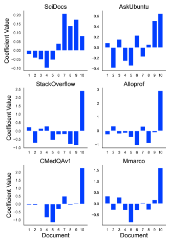
Figure 6: Domain adaptation study. Coefficients of the $u_{\text{lin}}$ confidence function (model: ember-v1, metric: mAP). Recall that documents are sorted in increasing order of relevance scores. Therefore, document 10 corresponds to the document with highest relevance score while document 1 is the least relevant to the query.

Table 11: Extensive domain adaptation study. nAUCs (in %) for all reference-test relevant pairs (model: ember-v1, metric: mAP).

	Method	$u_{\text{max}}$	$u_{\text{std}}$	$u_{\text{1-2}}$	$u_{\text{lin}}$
Reference Set	Test Set
SciDocs	AskUbuntu	23.8	21.7	8.1	24.6
	StackOverflow	19.6	28.6	47.6	-10.0
	Alloprof	15.9	18.8	21.5	8.6
	CMedQAv1	27.0	26.9	21.3	17.6
	Mmarco	28.8	21.3	13.0	17.3
AskUbuntu	SciDocs	51.2	64.9	-4.3	62.8
	StackOverflow	19.6	28.6	47.6	26.5
	Alloprof	15.9	18.8	21.5	21.8
	CMedQAv1	27.0	26.9	21.3	30.1
	Mmarco	28.8	21.3	13.0	29.9
StackOverflow	SciDocs	51.2	64.9	-4.3	15.5
	AskUbuntu	23.8	21.7	8.1	15.1
	Alloprof	15.9	18.8	21.5	25.7
	CMedQAv1	27.0	26.9	21.3	28.8
	Mmarco	28.8	21.3	13.0	18.0
Alloprof	SciDocs	51.2	64.9	-4.3	34.1
	AskUbuntu	23.8	21.7	8.1	20.9
	StackOverflow	19.6	28.6	47.6	48.1
	CMedQAv1	27.0	26.9	21.3	32.7
	Mmarco	28.8	21.3	13.0	21.4
CMedQAv1	SciDocs	51.2	64.9	-4.3	55.9
	AskUbuntu	23.8	21.7	8.1	23.0
	StackOverflow	19.6	28.6	47.6	43.8
	Alloprof	15.9	18.8	21.5	27.5
	Mmarco	28.8	21.3	13.0	20.7
Mmarco	SciDocs	51.2	64.9	-4.3	44.9
	AskUbuntu	23.8	21.7	8.1	23.2
	StackOverflow	19.6	28.6	47.6	44.7
	Alloprof	15.9	18.8	21.5	28.1
	CMedQAv1	27.0	26.9	21.3	33.8

In this section, we provide additional results concerning domain adaptation. In particular, we propose to take a closer look at the coefficients of our $u_{\text{lin}}$ confidence function (Figure 6) and to relate this information to abstention performance on the whole benchmark (Table 11).

A simple observation that can be made from Figure 6 is that the value taken by the coefficients depends very strongly on the number of positive documents per instance (see Table 6). Indeed, when we look at the results for the SciDocs dataset (five positive documents per instance on average), we see that $u_{\text{lin}}$ has positive weights on the first five documents and negative weights on the last five. A similar observation can be made for the other five datasets.

These observations are corroborated by Table 11, which shows that domain adaptation works well when the average number of positive documents per instance is approximately the same (e.g., from StackOverflow to Alloprof). On the contrary, we can see that when calibration is performed on SciDocs, performance transfers much less well, since the rest of the datasets have a significantly lower number of positive documents per instance. We therefore stress again the importance of using a reference set drawn from the same distribution as the test instances to avoid this kind of pitfall, since we remind that the number of positive documents per instance is unknown to the user.

Appendix D Additional Reference-Based Confidence Functions

In this section, we introduce two other ways to tackle confidence assessment in a reference-based setting: classification-based and distance-based methods.

D.1 Classification-Based Approach

Confidence assessment can be seen as a classification problem in which the good instances constitute the positive class, the bad instances constitute the negative class and the rest belongs to a neutral class. We therefore need to slightly modify reference set $\mathcal{S}_{\bm{\theta}}$ (Equation 6) to make it suitable for the classification setting. We thus build

$$\begin{split}\mathcal{S}_{\bm{\theta}}^{\text{clf}}=\bigr{\{}\left(\mathbf{z},\mathbbm{1}_{\left\{y>m^{+}\right\}}-\mathbbm{1}_{\left\{y<m^{-}\right\}}\right)\ |\ \\ (\mathbf{z},y)\in\mathcal{S}_{\bm{\theta}}\bigl{\}}.\end{split}$$ (9)

where $m^{+}>m^{-}\in\mathbb{R}$ are the thresholds above and below which an instance is considered good and bad respectively. Then, we fit a probabilistic classifier $\pi:\mathbb{R}^{k}\rightarrow[0,1]^{3}$ on $\mathcal{S}_{\bm{\theta}}^{\text{clf}}$, taking a vector of sorted scores $s(\mathbf{z})\in\mathbb{R}^{k}$ as input and returning the estimated probabilities of $s(\mathbf{z})$ to belong to class $-1$ (bad instances), $0$ (average instances) and $1$ (good instances). We finally define confidence function $u_{\text{clf}}$ such that for a given unsorted vector of relevance scores $\mathbf{z}$, $u_{\text{clf}}(\mathbf{z})=\pi_{2}\left(s(\mathbf{z})\right)-\pi_{0}\left(s(\mathbf{z})\right)$ (probability that $\mathbf{z}$ stems from a good instance minus the probability that $\mathbf{z}$ stems from a bad instance). The higher $u_{\text{clf}}(\mathbf{z})$, the more confident we are that $\mathbf{z}\in\mathbb{R}^{k}$ stems from a good instance.

In this work, we use a logistic regressor Cox and Snell (1989) with $l_{2}$ regularization parameter $\lambda=0.1$, $u_{\text{log}}$, and consider by default that the top and bottom 25% of instances with respect to metric function $m$ represent the good and bad instances respectively. We challenge this parameter in Appendix D.4.

D.2 Distance-Based Approach

Confidence estimation can also be seen as a distance problem. While $u_{\text{lin}}$ and $u_{\text{log}}$ are fully supervised, it is possible to imagine a distance-based confidence function $u_{\text{dist}}$ that evaluates how close an instance is to the set of good instances and how far it is from the set of bad instances.

For this purpose, based on thresholds $m^{+}$ and $m^{-}$ defined in Section D.1, we build $\mathcal{Z}_{\bm{\theta}}^{+}$ and $\mathcal{Z}_{\bm{\theta}}^{-}$, the sets composed of good and bad instances respectively. Formally,

$$\begin{cases}\begin{aligned} \mathcal{Z}_{\bm{\theta}}^{+}=\left\{\mathbf{z}:(\mathbf{z},y)\in\mathcal{S}_{\bm{\theta}},\ y>m^{+}\right\}\\ \mathcal{Z}_{\bm{\theta}}^{-}=\left\{\mathbf{z}:(\mathbf{z},y)\in\mathcal{S}_{\bm{\theta}},\ y<m^{-}\right\}\end{aligned}.\end{cases}$$

Then, we construct a confidence scorer $u_{\text{dist}}$ based on the distributions observed in $\mathcal{Z}_{\bm{\theta}}^{+}$ and $\mathcal{Z}_{\bm{\theta}}^{-}$. We define $u_{\text{dist}}=\delta\left(s(\cdot),\mathcal{Z}_{\bm{\theta}}^{-}\right)-\delta\left(s(\cdot),\mathcal{Z}_{\bm{\theta}}^{+}\right)$ as the difference between the distance to the set of bad instances and the distance to the set of good instances. Intuitively, the higher $u_{\text{dist}}(\mathbf{z})$, the more confident we are that $\mathbf{z}$ stems from a good instance.

In this experiment, we rely on the Mahalanobis distance Mahalanobis (2018); Lee et al. (2018); Ren et al. (2021). We compute the Mahalanobis distance between set $\mathcal{Z}\subset\mathbb{R}^{k}$ and $\mathbf{z}\in\mathbb{R}^{k}$ as

$$\delta_{\text{mah}}\left(\mathbf{z},\mathcal{Z}\right)=\left(\mathbf{z}-\bm{\mu}_{\mathcal{Z}}\right)\Sigma_{\mathcal{Z}}^{-1}\left(\mathbf{z}-\bm{\mu}_{\mathcal{Z}}\right)^{T},$$

where $\bm{\mu}_{\mathcal{Z}}\in\mathbb{R}^{k}$ denotes the average vector of reference set $\mathcal{Z}$ and $\Sigma_{\mathcal{Z}}^{-1}\in\mathbb{R}^{k\times k}$ the inverse of its covariance matrix.

D.3 Experimental Results

Table 12: Abstention performance assessment. nAUCs (in %) averaged over the whole set of available models, for each method including $u_{\text{log}}$ and $u_{\text{mah}}$.

	Method	$u_{\text{max}}$	$u_{\text{std}}$	$u_{\text{1-2}}$	$u_{\text{lin}}$	$u_{\text{log}}$	$u_{\text{mah}}$
Dataset	Metric
SciDocs	mAP	49.2	58.7	4.7	65.4	68.8	65.8
	mNDCG	54.9	62.9	10.2	66.6	70.2	66.8
	mRR	80.2	80.3	41.3	80.5	78.1	65.6
AskUbuntu	mAP	24.1	16.2	7.3	22.0	20.0	10.1
	mNDCG	28.1	15.7	8.6	24.5	21.9	10.5
	mRR	32.7	16.6	14.0	26.2	24.2	11.3
StackOverflow	mAP	20.7	24.6	35.7	42.6	42.0	37.5
	mNDCG	21.0	25.0	35.6	42.6	42.1	37.4
	mRR	21.4	24.8	36.1	42.8	42.3	37.7
Alloprof	mAmP	16.6	17.0	19.3	29.7	29.4	25.1
	mNDCG	16.8	16.9	18.8	29.3	28.9	24.9
	mRR	16.9	16.7	19.1	28.9	28.7	24.3
CMedQAv1	mAP	24.4	23.3	22.3	30.6	29.1	25.7
	mNDCG	25.0	23.5	22.3	30.7	27.0	24.8
	mRR	26.5	24.2	23.4	31.5	30.3	25.5
Mmarco	mAP	30.1	31.0	39.4	34.0	24.9	22.7
	mNDCG	30.5	30.9	38.8	34.1	24.9	23.3
	mRR	30.1	31.0	39.6	34.3	23.5	22.8
Average	mAP	27.5	28.5	21.5	37.4	35.7	31.1
	mNDCG	29.4	29.1	22.4	38.0	35.8	31.3
	mRR	34.6	32.3	28.9	40.7	37.8	31.2

Table 12 shows the normalized AUCs averaged model-wise for each dataset of the benchmark. We globally see that $u_{\text{lin}}$ remains the best reference-based method, although $u_{\text{log}}$ and $u_{\text{mah}}$ both show satisfactory results, outperforming the reference-free baselines.

D.4 Impact of Instance Qualification

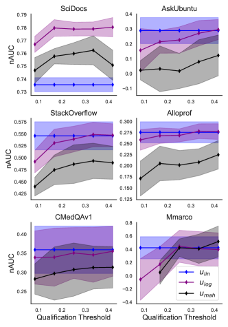
Figure 7: Instance qualification analysis. nAUC vs. instance quantile threshold for all datasets (model: ember-v1, metric: mAP).

In this section, we analyze the impact of the instance qualification threshold on the performance of the $u_{\text{log}}$ and $u_{\text{mah}}$ confidence functions. More precisely, the idea of this experiment is to vary the qualification threshold and to test the impact on nAUC over the whole benchmark. For the sake of readability, we present the results for the ember-v1 model and for the mAP only (see Figure 7).

The first observation we can make is that the confidence functions $u_{\text{log}}$ and $u_{\text{mah}}$ are sensitive to variations in the qualification threshold. For all the datasets presented, it is noticed that both methods performs better for thresholds between 30% and 40%. Intuitively, too low a threshold would lead to considering too few instances as good or bad, making it difficult to provide proper characterization and therefore resulting in less relevant confidence estimation. Conversely, a higher threshold creates less specific classes but with more instances, which seems to be better suited to our use case.

Additionally, while $u_{\text{mah}}$ performs less well overall than $u_{\text{lin}}$, $u_{\text{log}}$ competes fairly well when its qualification threshold is optimized. But the slight transformation required for the $\mathcal{S}_{\bm{\theta}}$ dataset (Equation 9) makes it a little less competitive in terms of computation time.

References

- Baek et al. (2023) Jinheon Baek, Soyeong Jeong, Minki Kang, Jong C Park, and Sung Ju Hwang. 2023. Knowledge-augmented language model verification. arXiv preprint arXiv:2310.12836.
- Bartlett and Wegkamp (2008) Peter L Bartlett and Marten H Wegkamp. 2008. Classification with a reject option using a hinge loss. Journal of Machine Learning Research, 9(8).
- Blundell et al. (2015) Charles Blundell, Julien Cornebise, Koray Kavukcuoglu, and Daan Wierstra. 2015. Weight uncertainty in neural network. In Proceedings of the 32nd International Conference on Machine Learning, volume 37 of Proceedings of Machine Learning Research, pages 1613–1622, Lille, France. PMLR.
- Bonifacio et al. (2021) Luiz Henrique Bonifacio, Vitor Jeronymo, Hugo Queiroz Abonizio, Israel Campiotti, Marzieh Fadaee, , Roberto Lotufo, and Rodrigo Nogueira. 2021. mmarco: A multilingual version of ms marco passage ranking dataset.
- Cheng et al. (2010) Weiwei Cheng, Michaël Rademaker, Bernard De Baets, and Eyke Hüllermeier. 2010. Predicting partial orders: ranking with abstention. In Machine Learning and Knowledge Discovery in Databases: European Conference, ECML PKDD 2010, Barcelona, Spain, September 20-24, 2010, Proceedings, Part I 21, pages 215–230. Springer.
- Chow (1957) Chi-Keung Chow. 1957. An optimum character recognition system using decision functions. IRE Transactions on Electronic Computers, (4):247–254.
- Cohan et al. (2020) Arman Cohan, Sergey Feldman, Iz Beltagy, Doug Downey, and Daniel S. Weld. 2020. Specter: Document-level representation learning using citation-informed transformers. In ACL.
- Colombo et al. (2022) Pierre Colombo, Eduardo Dadalto, Guillaume Staerman, Nathan Noiry, and Pablo Piantanida. 2022. Beyond mahalanobis distance for textual ood detection. Advances in Neural Information Processing Systems, 35:17744–17759.
- Colombo et al. (2023a) Pierre Colombo, Nathan Noiry, Guillaume Staerman, and Pablo Piantanida. 2023a. A novel information-theoretic objective to disentangle representations for fair classification. arXiv preprint arXiv:2310.13990.
- Colombo et al. (2023b) Pierre Colombo, Marine Picot, Nathan Noiry, Guillaume Staerman, and Pablo Piantanida. 2023b. Toward stronger textual attack detectors. arXiv preprint arXiv:2310.14001.
- Cortes et al. (2016) Corinna Cortes, Giulia DeSalvo, and Mehryar Mohri. 2016. Boosting with abstention. Advances in Neural Information Processing Systems, 29.
- Cox and Snell (1989) David Roxbee Cox and E Joyce Snell. 1989. Analysis of binary data, volume 32. CRC press.
- Cuconasu et al. (2024) Florin Cuconasu, Giovanni Trappolini, Federico Siciliano, Simone Filice, Cesare Campagnano, Yoelle Maarek, Nicola Tonellotto, and Fabrizio Silvestri. 2024. The power of noise: Redefining retrieval for rag systems.
- Darrin et al. (2022) Maxime Darrin, Pablo Piantanida, and Pierre Colombo. 2022. Rainproof: An umbrella to shield text generators from out-of-distribution data. arXiv preprint arXiv:2212.09171.
- Darrin et al. (2023) Maxime Darrin, Guillaume Staerman, Eduardo Dadalto Câmara Gomes, Jackie CK Cheung, Pablo Piantanida, and Pierre Colombo. 2023. Unsupervised layer-wise score aggregation for textual ood detection. arXiv preprint arXiv:2302.09852.
- El-Yaniv and Wiener (2010) Ran El-Yaniv and Yair Wiener. 2010. On the foundations of noise-free selective classification. Journal of Machine Learning Research, 11(53):1605–1641.
- Fisher (1922) Ronald A Fisher. 1922. The goodness of fit of regression formulae, and the distribution of regression coefficients. Journal of the Royal Statistical Society, 85(4):597–612.
- Gal et al. (2017) Yarin Gal, Riashat Islam, and Zoubin Ghahramani. 2017. Deep bayesian active learning with image data. In International conference on machine learning, pages 1183–1192. PMLR.
- Geifman and El-Yaniv (2017) Yonatan Geifman and Ran El-Yaniv. 2017. Selective classification for deep neural networks. In Advances in Neural Information Processing Systems, volume 30. Curran Associates, Inc.
- Geifman and El-Yaniv (2019) Yonatan Geifman and Ran El-Yaniv. 2019. SelectiveNet: A deep neural network with an integrated reject option. In Proceedings of the 36th International Conference on Machine Learning, volume 97 of Proceedings of Machine Learning Research, pages 2151–2159. PMLR.
- Gomes et al. (2022) Eduardo Dadalto Camara Gomes, Florence Alberge, Pierre Duhamel, and Pablo Piantanida. 2022. Igeood: An information geometry approach to out-of-distribution detection. arXiv preprint arXiv:2203.07798.
- Guerreiro et al. (2022) Nuno M Guerreiro, Pierre Colombo, Pablo Piantanida, and André FT Martins. 2022. Optimal transport for unsupervised hallucination detection in neural machine translation. arXiv preprint arXiv:2212.09631.
- Guo et al. (2016) Jiafeng Guo, Yixing Fan, Qingyao Ai, and W Bruce Croft. 2016. A deep relevance matching model for ad-hoc retrieval. In Proceedings of the 25th ACM international on conference on information and knowledge management, pages 55–64.
- Haroush et al. (2021) Matan Haroush, Tzviel Frostig, Ruth Heller, and Daniel Soudry. 2021. A statistical framework for efficient out of distribution detection in deep neural networks. arXiv preprint arXiv:2102.12967.
- Hein et al. (2019) Matthias Hein, Maksym Andriushchenko, and Julian Bitterwolf. 2019. Why relu networks yield high-confidence predictions far away from the training data and how to mitigate the problem. In Proceedings of the IEEE/CVF Conference on Computer Vision and Pattern Recognition, pages 41–50.
- Hendrycks and Gimpel (2016) Dan Hendrycks and Kevin Gimpel. 2016. A baseline for detecting misclassified and out-of-distribution examples in neural networks. arXiv preprint arXiv:1610.02136.
- Hoerl and Kennard (1970) Arthur E Hoerl and Robert W Kennard. 1970. Ridge regression: Biased estimation for nonorthogonal problems. Technometrics, 12(1):55–67.
- Houlsby et al. (2011) Neil Houlsby, Ferenc Huszár, Zoubin Ghahramani, and Máté Lengyel. 2011. Bayesian active learning for classification and preference learning. arXiv preprint arXiv:1112.5745.
- Hsu et al. (2020) Yen-Chang Hsu, Yilin Shen, Hongxia Jin, and Zsolt Kira. 2020. Generalized odin: Detecting out-of-distribution image without learning from out-of-distribution data. In Proceedings of the IEEE/CVF Conference on Computer Vision and Pattern Recognition, pages 10951–10960.
- Järvelin and Kekäläinen (2002) Kalervo Järvelin and Jaana Kekäläinen. 2002. Cumulated gain-based evaluation of ir techniques. ACM Transactions on Information Systems (TOIS), 20(4):422–446.
- Karpukhin et al. (2020) Vladimir Karpukhin, Barlas Oğuz, Sewon Min, Patrick Lewis, Ledell Wu, Sergey Edunov, Danqi Chen, and Wen-tau Yih. 2020. Dense passage retrieval for open-domain question answering. arXiv preprint arXiv:2004.04906.
- Khattab and Zaharia (2020) Omar Khattab and Matei Zaharia. 2020. Colbert: Efficient and effective passage search via contextualized late interaction over bert. In Proceedings of the 43rd International ACM SIGIR conference on research and development in Information Retrieval, pages 39–48.
- Lee et al. (2018) Kimin Lee, Kibok Lee, Honglak Lee, and Jinwoo Shin. 2018. A simple unified framework for detecting out-of-distribution samples and adversarial attacks. Advances in neural information processing systems, 31.
- Lefebvre-Brossard et al. (2023) Antoine Lefebvre-Brossard, Stephane Gazaille, and Michel C Desmarais. 2023. Alloprof: a new french question-answer education dataset and its use in an information retrieval case study. arXiv preprint arXiv:2302.07738.
- Lei et al. (2015) Tao Lei, Hrishikesh Joshi, Regina Barzilay, Tommi Jaakkola, Katerina Tymoshenko, Alessandro Moschitti, and Lluis Marquez. 2015. Semi-supervised question retrieval with gated convolutions. arXiv preprint arXiv:1512.05726.
- Lewis et al. (2020) Patrick Lewis, Ethan Perez, Aleksandra Piktus, Fabio Petroni, Vladimir Karpukhin, Naman Goyal, Heinrich Küttler, Mike Lewis, Wen-tau Yih, Tim Rocktäschel, et al. 2020. Retrieval-augmented generation for knowledge-intensive nlp tasks. Advances in Neural Information Processing Systems, 33:9459–9474.
- Lhoest et al. (2021) Quentin Lhoest, Albert Villanova del Moral, Yacine Jernite, Abhishek Thakur, Patrick von Platen, Suraj Patil, Julien Chaumond, Mariama Drame, Julien Plu, Lewis Tunstall, Joe Davison, Mario Šaško, Gunjan Chhablani, Bhavitvya Malik, Simon Brandeis, Teven Le Scao, Victor Sanh, Canwen Xu, Nicolas Patry, Angelina McMillan-Major, Philipp Schmid, Sylvain Gugger, Clément Delangue, Théo Matussière, Lysandre Debut, Stas Bekman, Pierric Cistac, Thibault Goehringer, Victor Mustar, François Lagunas, Alexander Rush, and Thomas Wolf. 2021. Datasets: A community library for natural language processing. In Proceedings of the 2021 Conference on Empirical Methods in Natural Language Processing: System Demonstrations, pages 175–184, Online and Punta Cana, Dominican Republic. Association for Computational Linguistics.
- Liu et al. (2020) Weitang Liu, Xiaoyun Wang, John Owens, and Yixuan Li. 2020. Energy-based out-of-distribution detection. Advances in neural information processing systems, 33:21464–21475.
- Loquercio et al. (2020) Antonio Loquercio, Mattia Segu, and Davide Scaramuzza. 2020. A general framework for uncertainty estimation in deep learning. IEEE Robotics and Automation Letters, 5(2):3153–3160.
- Mahalanobis (2018) Prasanta Chandra Mahalanobis. 2018. On the generalized distance in statistics. Sankhyā: The Indian Journal of Statistics, Series A (2008-), 80:S1–S7.
- Mao et al. (2023) Anqi Mao, Mehryar Mohri, and Yutao Zhong. 2023. Ranking with abstention. arXiv preprint arXiv:2307.02035.
- Mitra and Craswell (2017) Bhaskar Mitra and Nick Craswell. 2017. Neural models for information retrieval. arXiv preprint arXiv:1705.01509.
- Muennighoff et al. (2022) Niklas Muennighoff, Nouamane Tazi, Loïc Magne, and Nils Reimers. 2022. Mteb: Massive text embedding benchmark. arXiv preprint arXiv:2210.07316.
- Narayanan et al. (2012) Arvind Narayanan, Hristo Paskov, Neil Zhenqiang Gong, John Bethencourt, Emil Stefanov, Eui Chul Richard Shin, and Dawn Song. 2012. On the feasibility of internet-scale author identification. In 2012 IEEE Symposium on Security and Privacy, pages 300–314. IEEE.
- Neelakantan et al. (2022) Arvind Neelakantan, Tao Xu, Raul Puri, Alec Radford, Jesse Michael Han, Jerry Tworek, Qiming Yuan, Nikolas Tezak, Jong Wook Kim, Chris Hallacy, et al. 2022. Text and code embeddings by contrastive pre-training. arXiv preprint arXiv:2201.10005.
- Ni et al. (2021) Jianmo Ni, Chen Qu, Jing Lu, Zhuyun Dai, Gustavo Hernández Ábrego, Ji Ma, Vincent Y Zhao, Yi Luan, Keith B Hall, Ming-Wei Chang, et al. 2021. Large dual encoders are generalizable retrievers. arXiv preprint arXiv:2112.07899.
- Nogueira and Cho (2019) Rodrigo Nogueira and Kyunghyun Cho. 2019. Passage re-ranking with bert. arXiv preprint arXiv:1901.04085.
- Pedregosa et al. (2011) Fabian Pedregosa, Gaël Varoquaux, Alexandre Gramfort, Vincent Michel, Bertrand Thirion, Olivier Grisel, Mathieu Blondel, Peter Prettenhofer, Ron Weiss, Vincent Dubourg, et al. 2011. Scikit-learn: Machine learning in python. the Journal of machine Learning research, 12:2825–2830.
- Picot et al. (2022a) Marine Picot, Federica Granese, Guillaume Staerman, Marco Romanelli, Francisco Messina, Pablo Piantanida, and Pierre Colombo. 2022a. A halfspace-mass depth-based method for adversarial attack detection. Transactions on Machine Learning Research.
- Picot et al. (2022b) Marine Picot, Nathan Noiry, Pablo Piantanida, and Pierre Colombo. 2022b. Adversarial attack detection under realistic constraints.
- Picot et al. (2022c) Marine Picot, Guillaume Staerman, Federica Granese, Nathan Noiry, Francisco Messina, Pablo Piantanida, and Pierre Colombo. 2022c. A simple unsupervised data depth-based method to detect adversarial images.
- Podolskiy et al. (2021) Alexander Podolskiy, Dmitry Lipin, Andrey Bout, Ekaterina Artemova, and Irina Piontkovskaya. 2021. Revisiting mahalanobis distance for transformer-based out-of-domain detection. In Proceedings of the AAAI Conference on Artificial Intelligence, volume 35, pages 13675–13682.
- Rajpurkar et al. (2018) Pranav Rajpurkar, Robin Jia, and Percy Liang. 2018. Know what you don’t know: Unanswerable questions for squad. arXiv preprint arXiv:1806.03822.
- Ramos et al. (2003) Juan Ramos et al. 2003. Using tf-idf to determine word relevance in document queries. In Proceedings of the first instructional conference on machine learning, volume 242, pages 29–48. Citeseer.
- Reimers and Gurevych (2019) Nils Reimers and Iryna Gurevych. 2019. Sentence-bert: Sentence embeddings using siamese bert-networks. In Proceedings of the 2019 Conference on Empirical Methods in Natural Language Processing. Association for Computational Linguistics.
- Reimers and Gurevych (2021) Nils Reimers and Iryna Gurevych. 2021. The curse of dense low-dimensional information retrieval for large index sizes. In Proceedings of the 59th Annual Meeting of the Association for Computational Linguistics and the 11th International Joint Conference on Natural Language Processing (Volume 2: Short Papers), pages 605–611, Online. Association for Computational Linguistics.
- Ren et al. (2021) Jie Ren, Stanislav Fort, Jeremiah Liu, Abhijit Guha Roy, Shreyas Padhy, and Balaji Lakshminarayanan. 2021. A simple fix to mahalanobis distance for improving near-ood detection. arXiv preprint arXiv:2106.09022.
- Robertson et al. (2009) Stephen Robertson, Hugo Zaragoza, et al. 2009. The probabilistic relevance framework: Bm25 and beyond. Foundations and Trends® in Information Retrieval, 3(4):333–389.
- Robertson et al. (1995) Stephen E Robertson, Steve Walker, Susan Jones, Micheline M Hancock-Beaulieu, Mike Gatford, et al. 1995. Okapi at trec-3. Nist Special Publication Sp, 109:109.
- Smith and Gal (2018) Lewis Smith and Yarin Gal. 2018. Understanding measures of uncertainty for adversarial example detection. arXiv preprint arXiv:1803.08533.
- Staerman et al. (2021) Guillaume Staerman, Pavlo Mozharovskyi, Pierre Colombo, Stéphan Clémençon, and Florence d’Alché Buc. 2021. A pseudo-metric between probability distributions based on depth-trimmed regions. arXiv preprint arXiv:2103.12711.
- Thakur et al. (2021) Nandan Thakur, Nils Reimers, Andreas Rücklé, Abhishek Srivastava, and Iryna Gurevych. 2021. Beir: A heterogenous benchmark for zero-shot evaluation of information retrieval models. arXiv preprint arXiv:2104.08663.
- Voorhees et al. (1999) Ellen M Voorhees et al. 1999. The trec-8 question answering track report. In Trec, volume 99, pages 77–82.
- Wang et al. (2022) Liang Wang, Nan Yang, Xiaolong Huang, Binxing Jiao, Linjun Yang, Daxin Jiang, Rangan Majumder, and Furu Wei. 2022. Text embeddings by weakly-supervised contrastive pre-training. arXiv preprint arXiv:2212.03533.
- Wang et al. (2023) Zhiruo Wang, Jun Araki, Zhengbao Jiang, Md Rizwan Parvez, and Graham Neubig. 2023. Learning to filter context for retrieval-augmented generation. arXiv preprint arXiv:2311.08377.
- Xiao et al. (2023) Shitao Xiao, Zheng Liu, Peitian Zhang, and Niklas Muennighoff. 2023. C-pack: Packaged resources to advance general chinese embedding.
- Xin et al. (2021) Ji Xin, Raphael Tang, Yaoliang Yu, and Jimmy Lin. 2021. The art of abstention: Selective prediction and error regularization for natural language processing. In Proceedings of the 59th Annual Meeting of the Association for Computational Linguistics and the 11th International Joint Conference on Natural Language Processing (Volume 1: Long Papers), pages 1040–1051.
- Yoran et al. (2023) Ori Yoran, Tomer Wolfson, Ori Ram, and Jonathan Berant. 2023. Making retrieval-augmented language models robust to irrelevant context. arXiv preprint arXiv:2310.01558.
- Zeng et al. (2021) Zhiyuan Zeng, Keqing He, Yuanmeng Yan, Zijun Liu, Yanan Wu, Hong Xu, Huixing Jiang, and Weiran Xu. 2021. Modeling discriminative representations for out-of-domain detection with supervised contrastive learning. In Proceedings of the 59th Annual Meeting of the Association for Computational Linguistics and the 11th International Joint Conference on Natural Language Processing (Volume 2: Short Papers), pages 870–878, Online. Association for Computational Linguistics.
- Zhang et al. (2023) Peitian Zhang, Shitao Xiao, Zheng Liu, Zhicheng Dou, and Jian-Yun Nie. 2023. Retrieve anything to augment large language models.
- Zhang et al. (2017) Sheng Zhang, Xin Zhang, Hui Wang, Jiajun Cheng, Pei Li, and Zhaoyun Ding. 2017. Chinese medical question answer matching using end-to-end character-level multi-scale cnns. Applied Sciences, 7(8):767.
- Zhang et al. (2015) Yun Zhang, David Lo, Xin Xia, and Jian-Ling Sun. 2015. Multi-factor duplicate question detection in stack overflow. Journal of Computer Science and Technology, 30:981–997.
- Zhao et al. (2022) Wayne Xin Zhao, Jing Liu, Ruiyang Ren, and Ji-Rong Wen. 2022. Dense text retrieval based on pretrained language models: A survey. arXiv preprint arXiv:2211.14876.
- Zhu (2004) Mu Zhu. 2004. Recall, precision and average precision. Department of Statistics and Actuarial Science, University of Waterloo, Waterloo, 2(30):6.