On gravito-inertial surface waves

Yves Colin de Verdière Université Grenoble-Alpes, CNRS, Institut Fourier, 38000 Grenoble (France) yves.colin-de-verdiere@univ-grenoble-alpes.fr  and  Jérémie Vidal Université Grenoble-Alpes, CNRS, ISTerre, 38000 Grenoble (France) jeremie.vidal@univ-grenoble-alpes.fr This paper is dedicated to the memory of Steve.
(Date: Submitted February 2024)
Abstract.

In geophysical environments, wave motions that are shaped by the action of gravity and global rotation bear the name of gravito-inertial waves. We present a geometrical description of gravito-inertial surface waves, which are low-frequency waves existing in the presence of a solid boundary. We consider an idealized fluid model for an incompressible fluid enclosed in a smooth compact three-dimensional domain, subject to a constant rotation vector. The fluid is also stratified in density under a constant Brunt-Väisälä frequency. The spectral problem is formulated in terms of the pressure, which satisfies a Poincaré equation within the domain, and a Kelvin equation on the boundary. The Poincaré equation is elliptic when the wave frequency is small enough, such that we can use the Dirichlet-to-Neumann operator to reduce the Kelvin equation to a pseudo-differential equation on the boundary. We find that the wave energy is concentrated on the boundary for large covectors, and can exhibit surface wave attractors for generic domains. In an ellipsoid, we show that these waves are square-integrable and reduce to spherical harmonics on the boundary.

Key words and phrases:
Spectral theory, microlocal analysis, gravito-inertial waves, surface waves.
2020 Mathematics Subject Classification:
Primary 53Z05, 35Q35; Secondary 76U60, 76B70
JV received funding from European Research Council (erc) under the European Union’s Horizon 2020 research and innovation programme (grant agreement no. 847433, theia project).

1. Introduction

Global rotation and buoyancy are ubiquitous ingredients of many geophysical systems (e.g. the Earth’s oceans, or the liquid cores of planets). When the density stratification is stable (i.e. when a light fluid lies above a denser one), the Coriolis and buoyancy forces can sustain gravito-inertial waves. Since these waves are often believed to be key to understand the dynamics of geophysical flows, they have received considerable interest. From a mathematical viewpoint, these waves are governed by a mixed hyperbolic-elliptic equation [FS82a], which is referred to as the Poincaré equation below. Indeed, the latter reduces to the so-called Poincaré equation (denoted by Cartan [Car22] after the seminal work of poincaré [Poi85]) for pure inertial waves without density stratification [CdVV23]. Let us consider the simplest case (known as the $f-$plane approximation in geophysical modeling), where the fluid is subject to a constant global rotation $\overrightarrow{\Omega}=(f/2)\overrightarrow{e}_{3}$ and stratified in density with a constant Brunt-Väisälä frequency $N$ under the constant gravity $\overrightarrow{g}=-g\overrightarrow{e}_{3}$. In unbounded fluids, the angular frequency $\omega\in\mathbb{R}\setminus 0$ of gravito-inertial waves is then given by

(1.1) $$\omega||\boldsymbol{\xi}||^{2}=N^{2}(\xi_{1}^{2}+\xi_{2})^{2}+f^{2}\xi_{3}^{2},\quad\boldsymbol{\xi}=(\xi_{1},\xi_{2},\xi_{3}),$$

which is obtained when the principal symbol of the Poincaré equation vanishes. Dispersion relation (1.1) shows that gravito-inertial waves only exist when $\min(N,f)\leq|\omega|\leq\max(N,f)$. Hence, there is a frequency gap without waves when the fluid is unbounded. However, low-frequency gravito-inertial waves can exist in this frequency gap when the fluid domain is bounded [FS82a]. Motivated by geophysical applications, we recently revisited this canonical problem and (surprisingly) found these low-frequency waves are polynomials when the boundary is an ellipsoid [VCdV24].

The goal of this study is to present a geometrical description of these gravito-inertial surface waves, which are denoted below by Kelvin waves. Indeed, they share similar properties with surface waves studied by Lord Kelvin in oceanography [Kel80]. This is based on a reduction to the boundary of the wave equations, following our previous works on inertial [CdVV23] and gravito-inertial waves [VCdV24]. We consider an incompressible fluid in a smooth compact three-dimensional (3D) domain $D$, which is subject to a constant global rotation. The fluid is also supposed to be stably stratified in density with a constant Brunt-Väisälä frequency $N$. The motion of the fluid can be recovered from the pressure $\phi$, which satisfies a Poincaré equation inside $D$, and a Kelvin equation on the boundary $\partial D$. If the frequency $\omega$ is small enough, the Poincaré equation is elliptic. Thus, we can use the Dirichlet-to-Neumann operator (see Appendix B) to reduce the Kelvin equation to a pseudo-differential equation on the boundary. In this case, the eigensolutions concentrate on the boundary for large covectors (i.e. large wave numbers in the physical terminology).

The manuscript is organized as follows. We first present general properties of the Poincaré and Kelvin equations in §2 and §3. Then, a detailed derivation of the Kelvin equation is given in §4. Next, a microlocal analysis of the Kelvin equation is presented in §5 and §6. Finally, the case where $\partial D$ is an ellipsoid is considered in §7. Notably, we show that the spectrum is pure point with polynomial eigenvectors, and that the pressure field reduces to a spherical harmonic on $\partial D$.

2. The Poincaré operator

We consider a fluid in a compact domain $D\subset\mathbb{R}^{3}$ with a smooth boundary $\partial D$, and we equip $\mathbb{R}^{3}$ with the canonical (orthogonal) basis vectors $(\overrightarrow{e}_{1},\overrightarrow{e}_{2},\overrightarrow{e}_{3})$. We assume that the fluid domain is submitted to a constant global rotation $\overrightarrow{\Omega}$ (with respect to an inertial frame), and that the fluid is stably stratified in density with a Brunt-Väisälä frequency $N>0$ under the imposed gravity $\overrightarrow{g}=-g\overrightarrow{e}_{3}$. In this paper, we always assume that $\overrightarrow{g}$ and $N$ are constant. We seek small-amplitude periodic motions, with angular frequency $\omega$, with respect to a hydrostatic reference configuration. We refer the interested reader to [VCdV24] for further details about the physical model. In the linear theory, the equations in the rotating frame are

(2.1) $$i\omega\overrightarrow{u}+2\overrightarrow{\Omega}\wedge\overrightarrow{u}-\rho\overrightarrow{g}=-\nabla\phi,\quad\mathrm{div}\overrightarrow{u}=0,\quad i\omega\rho=N^{2}u_{3}/g,$$

where the velocity vector field $\overrightarrow{u}$ is tangent to the boundary $\partial D$, where $\phi$ is the pressure, and $\rho$ is the density perturbation. We can rewrite these equations in a symmetric form as

(2.2) $$i\omega\overrightarrow{u}+2\overrightarrow{\Omega}\wedge\overrightarrow{u}+N\rho_{1}\overrightarrow{e}_{3}=-\nabla\phi,\quad\mathrm{div}\overrightarrow{u}=0,\quad i\omega\rho_{1}=Nu_{3},$$

where $\rho_{1}:=\rho g/N$ is a rescaled density of the fluid.

Using the Leray projector denoted by $\Pi$ (see Appendix A) and defining $\Pi_{0}$ the operator acting on a pair $(\overrightarrow{u},\rho)$ by

$$\Pi_{0}(\overrightarrow{u},\rho_{1}):=(\Pi\overrightarrow{u},\rho_{1}),$$

we can reformulate the spectral problem as the spectral properties of the Poincaré operator $\mathcal{P}$ defined by

(2.3) $${\mathcal{P}}:=i\Pi_{0}A\Pi_{0},\quad A=\left(\begin{matrix}0&-2\Omega_{3}&2\Omega_{2}&0\\ 2\Omega_{3}&0&-2\Omega_{1}&0\\ -2\Omega_{2}&2\Omega_{1}&0&N\\ 0&0&-N&0\end{matrix}\right),$$

where $iA$ is self-adjoint on $L^{2}(D,{\mathbb{C}}^{4})$. The eigenvalues of $iA$ are $\pm\omega_{\pm}$ with

(2.4) $$\omega_{\pm}=\sqrt{\frac{1}{2}\left(N^{2}+f^{2}\pm\sqrt{(N^{2}+f^{2})^{2}-16N^{2}\Omega_{3}^{2}}\right)},$$

where we have introduced $f:=2\|\overrightarrow{\Omega}\|$ (which is called the Coriolis parameter in the geophysical literature). Then, the spectrum of $\mathcal{P}$ (i.e. the set of values of $\omega$ for which $\mathcal{P}-\omega I$ is not invertible, where $I$ is the identity operator) is given by the following theorem.

Theorem 2.1.

The Poincaré operator $\mathcal{P}$ is a bounded self-adjoint operator in $L^{2}(D,\mathbb{C}^{4})$, and its spectrum $\sigma(\mathcal{P})$ is given by

$$\sigma(\mathcal{P})=[-\omega_{+},\omega_{+}].$$
Proof.

We have $\|\Pi_{0}\|=1$, while the eigenvalues of the Hermitian matrix $iA$ are $\pm\omega_{\pm}$. This proves that $\|\mathcal{P}\|\leq\omega_{+}$. Moreover, $\mathcal{P}$ is not elliptic when $\omega_{-}\leq|\omega|\leq\omega_{+}$, and we will see in Section 5.3 that the Kelvin equation is not elliptic for $0<|\omega|<\omega_{-}$. The theorem follows from these observations and Appendix C (see also Theorem 2.1. of [CdV20]). ∎

Our main interest in this paper will be the study of $\sigma(\mathcal{P})\cap]-\omega_{-},\omega_{-}[$. The low-frequency waves in this interval are refereed as class-II solutions in [FS82a]. This part of the spectrum is controlled by an equation $K_{\omega}\phi=0$ satisfied by the pressure on the boundary, which we call the Kelvin equation. The solutions of the Kelvin equation for large covectors are localized on the boundary. This shows that these solutions are associated with surface waves of the Poincaré operator.

3. Equations for the boundary value of the pressure

We want to recast the equations for the velocity $\overrightarrow{u}$ and the density $\rho_{1}$ as a boundary-value problem for the scalar pressure $\phi$. Indeed, this will ease the microlocal analysis of the problem. The pressure satisfies an equation in $D$, called the Poincaré equation, and boundary conditions given by the Kelvin equation. We explain below how to obtain these two equations in the general case.

3.1. Poincaré equation

When $\omega\neq\pm\omega_{\pm}$, we can solve the equation

(3.1) $$\overrightarrow{u}=M_{\omega}(i\nabla\phi)$$

with $M_{\omega}=j^{\star}(\omega-iA)^{-1}j$ where $j:{\mathbb{R}}^{3}\rightarrow{\mathbb{R}}^{4}$ is the injection $\overrightarrow{u}\rightarrow(\overrightarrow{u},0)^{\top}$. Then, we make use of the divergenceless condition ${\rm div}(\overrightarrow{u})=0$ to obtain the Poincaré equation $P_{\omega}\phi=0$ for $\phi$. This is a partial differential equation of degree two with constant coefficients, which is given by

(3.2) $$P_{\omega}\phi=\omega\left((\omega^{2}-N^{2})\Delta+N^{2}\frac{\partial^{2}}{\partial x_{3}^{2}}-4\left(\sum_{i=1}^{3}\Omega_{i}\frac{\partial}{\partial x_{i}}\right)^{2}\right)\phi.$$

Note that, if we do that directly, the equation that we obtain has a simple zero at $\omega=0$. Equation (3.2) is also defined using a determinant as

$$P_{\omega}\phi=-\begin{vmatrix}\omega-iA&\begin{pmatrix}\partial_{1}\\ \partial_{2}\\ \partial_{3}\\ 0\end{pmatrix}\\ \begin{pmatrix}\partial_{1}&\partial_{2}&\partial_{3}&0\end{pmatrix}&0\end{vmatrix}\phi$$

The symbol of $P_{\omega}$ is

$$\sigma_{\omega}(\boldsymbol{\xi})=\omega\left((N^{2}-\omega^{2})\|\boldsymbol{\xi}\|^{2}-N^{2}\xi_{3}^{2}+4\left(\boldsymbol{\xi}.\overrightarrow{\Omega}\right)^{2}\right),$$

where $\boldsymbol{\xi}=(\xi_{1},\xi_{2},\xi_{3})$ is the covector of norm $||\boldsymbol{\xi}||=(\xi_{1}^{2}+\xi_{2}^{2}+\xi_{3}^{2})^{1/2}$. We also define the real-valued matrix $\Sigma_{\omega}$, associated with the quadratic form $\sigma_{\omega}$, as

$$\sigma_{\omega}(\boldsymbol{\xi}):=\langle\Sigma_{\omega}\boldsymbol{\xi}|\boldsymbol{\xi}\rangle$$

where $\langle.|.\rangle$ is the canonical duality product. If $0<\omega<\omega_{-}$, $\Sigma_{\omega}$ is a real-valued, symmetric, and strictly positive matrix. The Poincaré operator is elliptic if and only if $0<|\omega|<\omega_{-}$ or $|\omega|>\omega_{+}$.

3.2. Kelvin equation

Using again the equation $\overrightarrow{u}=M_{\omega}(i\nabla\phi)$, we write that $\overrightarrow{u}$ is tangent to $\partial D$. This allows us to obtain the Kelvin equation. Since this equation is quite complicated in general, we will compute it in some special cases (see §4). In the general case, the Kelvin equation can be written as a pseudo-differential equation $K_{\omega}\phi=0$ on the boundary $\partial D$, which satisfies Theorem 3.1.

Theorem 3.1.

The Poincaré equation is elliptic when $0<|\omega|<\omega_{-}$, and the Kelvin equation reads

(3.3) $$K_{\omega}\phi=DtN_{\omega}\phi+i\overrightarrow{W}_{\omega}\phi,$$

where the Dirichlet to Neumann operator $DtN_{\omega}$ (see Appendix B) is defined using the Euclidian metric $g_{\omega}$ associated to the symbol $\sigma_{\omega}$ of $P_{\omega}$, that is $g_{\omega}=\Sigma_{\omega}^{-1}$, and $\overrightarrow{W}_{\omega}$ is a real-valued vector field tangent to the boundary. Moreover, $\overrightarrow{W}_{\omega}$ is divergenceless with respect to the area $v_{\omega}$ associated to the restriction $g_{\omega,\partial}$ of $g_{\omega}$ to $\partial D$. In particular, $K_{\omega}$ is a self-adjoint pseudo-differential operator  of degree $1$ on $L^{2}(\partial D,v_{\omega})$ whose principal symbol is

(3.4) $$k_{\omega}(x,\boldsymbol{\xi})=\sqrt{g_{\omega,\partial}^{\star}(x,\boldsymbol{\xi})}-\langle\boldsymbol{\xi}|\overrightarrow{W}_{\omega}(x)\rangle,$$

where $(x,\boldsymbol{\xi})\in T^{\star}(\partial D)$ and $g_{\omega,\partial}^{\star}$ is the dual of $g_{\omega,\partial}$. The Kelvin equation $K_{\omega}\phi=0$ is elliptic at $x\in\partial D$ if and only if $\|\overrightarrow{W}_{\omega}(x)\|_{g_{\omega,\partial}}<1$.

Proof.

For any two smooth functions $\phi_{1}$ and $\phi_{2}$ on $D$, let us consider the Hermitian bracket

$$((\phi_{1}|\phi_{2}))=\langle i\nabla\phi_{1}|M_{\omega}(i\nabla\phi_{2})\rangle_{L^{2}}$$

where $\langle u_{1}|u_{2}\rangle_{L^{2}}=\int_{D}u_{1}\cdot\overline{u}_{2}\,|dx|$ where $\overline{u}$ is the complex conjugate of $u$. Integrating by part, we get

$$((\phi_{1}|\phi_{2}))=-\int_{D}\phi_{1}\overline{{\rm div}\left(M_{\omega}\nabla\phi_{2}\right)}\,|dx|+\int_{\partial D}\phi_{1}\overline{L_{\omega}{\phi}_{2}}\,v_{\omega}$$

where $L_{\omega}$ is a complex-valued vector field. Let us assume now that $P_{\omega}\phi_{2}=0$, and we get

$$((\phi_{1}|\phi_{2}))=\int_{\partial D}\phi_{1}\overline{L_{\omega}{\phi}_{2}}\,v_{\omega}$$

This vanishes if and only if $M_{\omega}(\nabla\phi_{2})$ is orthogonal to all gradient fields and, hence, is tangent to the boundary. In other words, the equation $L_{\omega}\phi=0$ is the boundary condition for $\phi$, that is the Kelvin equation. Assuming also that $P_{\omega}\phi_{1}=0$, we see that $L_{\omega}$ is self-adjoint. We can always decompose the vector field $L_{\omega}$ as $\Psi\overrightarrow{n}_{\omega}+i\overrightarrow{W}_{1}$ where $\Psi$ is a function, $\overrightarrow{n}_{\omega}$ is the unit outgoing normal to $\partial D$ for the metric $g_{\omega}$, and $\overrightarrow{W}$ is a complex vector field tangent to $\partial D$. Then, we can rewrite $L_{\omega}$ as $L_{\omega}=\Psi DtN_{\omega}+i\overrightarrow{W}_{1}$. The self-adjointness of the operator $L_{\omega}$ implies that the principal symbol is real-valued. $\Psi$ is thus real-valued, and $\overrightarrow{W}_{1}$ is a real-valued vector field. Taking the adjoint, we get

$$L_{\omega}=L_{\omega}^{\star}=DtN_{\omega}\Psi+i\overrightarrow{W}_{1}+i{\rm div}_{\omega}(\overrightarrow{W}_{1}).$$

This implies, by separation of the real and imaginary parts, that ${\rm div}_{\omega}(\overrightarrow{W}_{1})=0$ and $\Psi DtN_{\omega}-DtN_{\omega}\Psi=0$. The last equation implies that $\Psi:\partial D\rightarrow{\mathbb{R}}$ is invariant by the geodesic flow of $g_{\omega,\partial}$ and, hence, constant. Removing this real constant, we get the final result. ∎

4. Computing the Kelvin equation

Let us fix a point $x\in\partial D$, and we assume that the tangent plane to $\partial D$ is given by $a_{1}x_{1}+a_{2}x_{2}+a_{3}x_{3}=0$ where $\boldsymbol{a}=(a_{1},a_{2},a_{3})$ is a non zero outward normal covector of $D$. The condition that $\overrightarrow{u}$ is tangent on $\partial D$ can be written as a vanishing condition for the determinant given by

(4.1) $$B_{\omega}(\nabla\phi,\boldsymbol{a})=\begin{vmatrix}\omega-iA&\begin{pmatrix}\partial_{1}\phi\\ \partial_{2}\phi\\ \partial_{3}\phi\\ 0\end{pmatrix}\\ \begin{pmatrix}a_{1}&a_{2}&a_{3}&0\end{pmatrix}&0\end{vmatrix}.$$

The Hermitian form $B_{\omega}$ can be written as $B_{\omega}=\Sigma_{\omega}+i\Xi_{\omega}$, where $\Xi$ is real and antisymmetric. We can rewrite $B_{\omega}(\nabla\phi,\boldsymbol{a})$ as a complex-valued vector field acting on $\phi$, which gives

$$B_{\omega}(\nabla\phi,\overrightarrow{a})=\left(\overrightarrow{N}+i\overrightarrow{W}_{1}\right)\phi$$

with $\overrightarrow{N}=\Sigma_{\omega}(\boldsymbol{a})$. Using the fact that $g_{\omega}=\Sigma_{\omega}^{-1}$, we get

$$g_{\omega}(\overrightarrow{N},\overrightarrow{e})=\langle\boldsymbol{a}|\overrightarrow{e}\rangle.$$

This confirms that $\overrightarrow{N}$ is $g_{\omega}$-orthogonal to $\partial D$. We see that the vector $\overrightarrow{N}$ is outward because, if $\overrightarrow{n}$ is an outgoing vector, $g_{\omega}(\overrightarrow{N},\overrightarrow{n})=\langle\boldsymbol{a}|\overrightarrow{n}\rangle$ is positive. Moreover, we have

$$g_{\omega}(\overrightarrow{N},\overrightarrow{N})=\langle\boldsymbol{a}|\overrightarrow{N}\rangle=\sigma_{\omega}(\boldsymbol{a}).$$

Hence, we have $\overrightarrow{N}=\sqrt{\sigma_{\omega}(\boldsymbol{a})}\overrightarrow{n}_{\omega}$. Finally, we get the Kelvin equation

$$\sqrt{\sigma_{\omega}(\boldsymbol{a})}DtN_{\omega}\phi+i\overrightarrow{W}_{1}\phi=0,$$

which is of the form (3.3) with $\overrightarrow{W}=\overrightarrow{W}_{1}/\sqrt{\sigma_{\omega}(\boldsymbol{a})}$.

The Kelvin equation is non-elliptic at points where the tangent plane is given by $\boldsymbol{a}$ if and only if

$$\|\overrightarrow{W}_{1}\|_{\omega}^{2}>\sigma_{\omega}(\boldsymbol{a}).$$

At the points $x\in\partial D$ such that $\overrightarrow{W}_{1}(x)\neq 0$ for $\omega=0$, this holds when $\omega$ is small enough. Indeed, there is a coefficient $1/\omega$ in front of $g_{\omega}$ and a coefficient $\omega$ in front of $\sigma(\omega)$. Note also that $DtN_{\omega}$ and $\overrightarrow{W}_{1}$ are even functions of $\omega$ such that, if $K_{\omega}\phi=0$, we have $K_{-\omega}\bar{\phi}=0$. This allows us to obtain, as expected, real-valued eigenvectors.

5. Explicit computations

Refer to caption
Figure 1. Non-ellipticity of the Kelvin equation for different cases. Left: Aligned case with $\overrightarrow{\Omega}\propto\overrightarrow{g}$. The Kelvin equation is non-elliptic near the equator when $\cos\phi\leq\omega/N$ (see §5.1). Right: The Kelvin equation is elliptic when the tangent plane (gray) is parallel to gravity (see §5.2), whereas it is non-elliptic when the tangent plane is orthogonal to gravity (see §5.3).

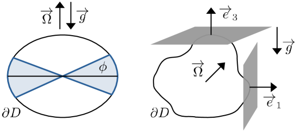
As illustrated in figure 1, we seek below whether the Kelvin equation is elliptic or not for different cases. To check the ellipticity of $K_{\omega}$, we need to compute the Hermitian form $B_{\omega}$ and the metric $g_{\omega}$. Without loss of generality, we can assume that $\overrightarrow{\Omega}=(\Omega_{1},0,\Omega_{3})^{\top}$ with $f^{2}=4(\Omega_{1}^{2}+\Omega_{3}^{2})$. The symbol of the Poincaré equation is written as

$$\sigma_{\omega}(\boldsymbol{\xi})=\omega\left[(N^{2}+4\Omega_{1}^{2}-\omega^{2})\xi_{1}^{2}+(N^{2}-\omega^{2})\xi_{2}^{2}+(4\Omega_{3}^{2}-\omega^{2})\xi_{3}^{2}+8\Omega_{1}\Omega_{3}\xi_{1}\xi_{3}\right]$$

with $\boldsymbol{\xi}=(\xi_{1},\xi_{2},\xi_{3})$, and the associated metric is

$$g_{\omega}=\frac{1}{\delta\omega}\left((4\Omega_{3}^{2}-\omega^{2})dx_{1}^{2}+(N^{2}+4\Omega_{1}^{2}-\omega^{2})dx_{3}^{2}-8\Omega_{1}\Omega_{3}dx_{1}dx_{3}\right)+\frac{dx_{2}^{2}}{\omega(N^{2}-\omega^{2})}.$$

with $\delta=(\omega^{2}-\omega_{-}^{2})(\omega^{2}-\omega_{+}^{2})$. Moreover, we have

$$\overrightarrow{W}_{1}=2\Omega_{3}(N^{2}-\omega^{2})(a_{1}\partial_{2}-a_{2}\partial_{1})+2\Omega_{1}\omega^{2}(a_{2}\partial_{3}-a_{3}\partial_{2}),$$

which is obtained from equation (4.1). We see that $\overrightarrow{W}_{1}$ is everywhere transverse to the meridians. This implies the wave propagation in the prograde direction (e.g. is eastward when $\Omega_{3}>0$). When $\omega$ is small, we also have

$$\overrightarrow{W}_{1}=2\Omega_{3}N^{2}(a_{1}\partial_{2}-a_{2}\partial_{1})+\mathcal{O}(\omega^{2})$$

and $\overrightarrow{W}=\overrightarrow{W_{1}}/\sqrt{\sigma_{\omega}(\boldsymbol{a})}$. We can now evaluate these formulas for different cases.

5.1. Vertical stratification and rotation

We describe here the Kelvin equation when the rotation vector $\overrightarrow{\Omega}$ is parallel to gravity (known as the $f-$plane approximation in geophysical literature). The corresponding Kelvin equation was derived in [FS82a], and revisited in [VCdV24] using microlocal arguments when $\partial D$ is an ellipsoid. We have $\Omega_{1}=0$ and define the Coriolis parameter $f:=2\Omega_{3}$ such that

$$\omega_{-}=\min(N,f),\quad\omega_{+}=\max(N,f),$$

and $\delta=(\omega^{2}-N^{2})(\omega^{2}-f^{2})$. The problem is then invariant by rotation around the $x_{3}$-axis. Hence, we can assume that $\boldsymbol{a}=(\cos\phi,0,\sin\phi)$ with $|\phi|\leq\pi/2$, where $\phi$ can be called the latitude. Then, we get

$$\sigma_{\omega}(\boldsymbol{a})=\omega\left[(N^{2}-\omega^{2})\cos^{2}\phi+(f^{2}-\omega^{2})\sin^{2}\phi\right]$$

and

$$\overrightarrow{W}_{1}=f(N^{2}-\omega^{2})\cos\phi\partial_{2},\quad\|\overrightarrow{W}_{1}\|_{\omega}^{2}=\frac{f^{2}(N^{2}-\omega^{2})^{2}\cos^{2}\phi}{\omega(N^{2}-\omega^{2})}.$$

We can check that the Kelvin equation is elliptic at large latitudes, that is when $|\cos\phi|<\omega/N$. In particular, the operator is never elliptic at the equator $\phi=0$.

We can also compute the symbol of $k_{\omega}$ of $K_{\omega}$. It is given by

$$k_{\omega}(x,\boldsymbol{\xi})=\omega+N\cos\phi(x)\frac{\xi_{s}}{\sqrt{\xi_{s}^{2}+\xi_{u}^{2}}},$$

where $\boldsymbol{\xi}=(\xi_{s},\xi_{u})$ are the canonical coordinates of $\boldsymbol{\xi}$ in an orthonormal basis of $T_{x}\partial D$ with $x_{s}$ a length parametrisation of the “parallel” through $x$ oriented to the “east” (i.e. in the prograde direction when $f>0$). In particular, we see that

  • When $0<N\leq f$, $T^{\star}\partial D\setminus 0$ is foliated by the cones $H^{-1}(\omega)$ with $|\omega|\leq\omega_{-}=N$.

  • When $0<f<N$, we have

    $$\cup_{|\omega|\leq f}H^{-1}(\omega)=\left\{\left|\cos\phi\frac{\xi_{s}}{\sqrt{\xi_{s}^{2}+\xi_{u}^{2}}}\right|\leq f/N\right\},$$

    which is not the full cotangent space. This will have some implications on the Weyl asymptotics for the eigenvalues when $\partial D$ is an ellipsoid.

5.2. Stratification parallel to the boundary

We consider the case where the tangent plane is horizontal $\{x_{3}\leq 0\}$, such that $\boldsymbol{a}=(0,0,1)$ and the stratification with $N>0$ is parallel to the tangent plane. Then, we have

$$\overrightarrow{W}_{1}=-2\Omega_{1}\omega^{2}\partial_{2},\quad\|\overrightarrow{W}_{1}\|_{\omega}^{2}=\frac{4\Omega_{1}^{2}\omega^{4}}{\omega(N^{2}-\omega^{2})},\quad\sigma_{\omega}(\boldsymbol{a})=\omega(4\Omega_{3}^{2}-\omega^{2}).$$

The ellipticity condition is given by

$$\|\overrightarrow{W}_{1}\|_{\omega}^{2}<\omega(4\Omega_{3}^{2}-\omega^{2}).$$

After some calculations, this gives

$$(\omega^{2}-\omega_{-}^{2})(\omega^{2}-\omega_{+}^{2})>0$$

which is satisfied when $0<|\omega|<\omega_{-}$. Hence, there are no surface waves in this case.

5.3. Stratification orthogonal to the boundary

We assume that $\boldsymbol{a}=(1,0,0)$ and $\Omega_{3}\neq 0$. Then, we have

$$\overrightarrow{W}_{1}=2(N^{2}-\omega^{2})\Omega_{3}\partial_{2},\quad\|\overrightarrow{W}_{1}\|_{\omega}^{2}=\frac{4(N^{2}-\omega^{2})\Omega_{3}^{2}}{\omega},\quad\sigma_{\omega}(\boldsymbol{a})=\omega(N^{2}+4\Omega_{1}^{2}-\omega^{2}).$$

After some calculations, this gives the ellipticity condition

$$(\omega^{2}-\omega_{-}^{2})(\omega^{2}-\omega_{+}^{2})<0.$$

We see that the Kelvin equation is non-elliptic when $0<|\omega|<\omega_{-}$. Hence, there are always surface waves located near the equator. This completes the fact that the spectrum is always $[-\omega_{+},\omega_{+}]$, as stated in Theorem 2.1.

6. Dynamics of waves

We can study a more general problem. Let $(X,g)$ be a closed Riemannian surface, and $\overrightarrow{W}$ be a divergenceless vector field on $X$. We consider a self-adjoint operator $K$ defined by

$$K=E-\frac{1}{i}\overrightarrow{W},$$

where $E$ is an elliptic self-adjoint pseudo-differential operator of principal symbol $e$ of degree $1$. The principal symbol $k$ of $K$ is given by

$$k(x,\boldsymbol{\xi})=e(x,\boldsymbol{\xi})-\langle\boldsymbol{\xi}|\overrightarrow{W}(x)\rangle.$$

If the characteristic cone $\Sigma=k^{-1}(0)$ is non-degenerate, $K$ is called of principal type. The projection on $X$ of $\Sigma$ is $S=\pi_{M}(\Sigma=\{\|\overrightarrow{W}\|_{g}\geq 1\}$. For each $x\in\partial D$ such that $\|\overrightarrow{W}(x)\|_{g}>1$, there is exactly two covectors directions in $\Sigma$. The base of the cone $\Sigma$ consists of two copies of $S$ glued along the boundaries $\{\|\overrightarrow{W}\|_{g}=1\}$. If the Hamiltonian vector field is non-radial on $\Sigma$, this basis is the union of 2D-tori (because it supports a non-vanishing vector field: the unscaled Hamiltonian field of the symbol).

If $k$ is allowed to smoothly vary as a function of a spectral parameter $\omega$ (e.g. $k_{\omega}$ in the previous sections), the projection of the classical (the group velocity) dynamics (the group velocity) onto $X$ is given by

$$\left(\frac{\partial k_{\omega}}{\partial\omega}\right)^{-1}\left(\overrightarrow{G}+\overrightarrow{W}\right),$$

where $\overrightarrow{G}$ is the projection of the geodesic field for the corresponding values of $\xi$. The main direction is then given by $\pm\overrightarrow{W}$ with $\pm=$sign $\frac{\partial k_{\omega}}{\partial\omega}$. This gives the motion to the east in our case, at least for small values of $\omega$.

We can apply the study of attractors initiated in [CdVSR20, CdV20]. We assume that the Hamiltonian flow of $k$ satisfies the Morse-Smale assumptions of [CdVSR20]. Then, the solutions of the Kelvin equation are Lagrangian distributions located over the attractors and the repulsors. In the case of the Kelvin equation, we thus predict the existence of some attractors for the surface waves (which remain to be observed in physics).

7. The case of ellipsoids
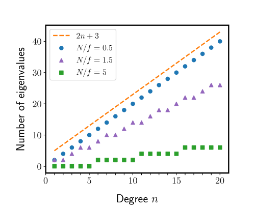
Refer to caption
Figure 2. Number of eigenvalues in the interval $0<|\omega|<\omega_{-}$ for polynomial eigenvectors of degree less than $n$. Aligned rotation and gravity (as considered in §5.1) when $\partial D$ is a sphere. For every degree $n$, the number of eigenvalues is bounded by the number $2n+3$ of spherical harmonics of degree $n+1$. Numerical calculations following the method presented in [VCdV24].

Now, we assume that $\partial D$ is an ellipsoid. Ellipsoidal models have proven useful for geophysical applications (e.g. to model some peculiar vortices in the Earth’s oceans [VCdV24]). In an ellipsoid, the spectrum of the Poincaré operator is pure-point and dense in $[-\omega_{+},\omega_{+}]$, with polynomial eigenvectors. In particular, gravito-inertial surface modes were found in [VCdV24] when $0<|\omega|<\omega_{-}$. Numerical calculations (figure 2) show that the number of eigenvalues associated with each polynomial vector space of degree $n$ is bounded by $2n+3$, which is the number of spherical harmonics of degree $n+1$. Indeed, if the velocity $\overrightarrow{u}$ is of degree $n\geq 1$, then the pressure $\phi$ is of degree $n+1$ according to equation (3.1). This strongly suggests a connection, when $\partial D$ is an ellipsoid, between the gravito-inertial surface modes and the theory of spherical harmonics. This is the subject of the subsection 7.1. Moreover, the numerical results also confirm the microlocal predictions detailed in §5.1, which show that the surface waves do not span the full cotangent space when $N\geq f$. Another natural question is thus to estimate, when the polynomial degree $n$ tends to infinity, the asymptotic number of eigenvalues of the Poincaré operator in the interval $]0,\omega_{-}[$. A conjecture for this question is given in Section 8.

7.1. Spherical harmonics

We consider the case of an ellipsoid $E:=L(B)$, where $B$ is the unit Euclidean ball and $L$ is linear. The pull-back of the Poincaré operator to $B$ is then of the form ${\mathcal{P}}_{E}=\Pi_{E}C_{E}\Pi_{E}$ where $C_{E}$ is a $4\times 4$ matrix and $\Pi_{E}$ is the Leray projector for the pull-back metric $L^{\star}(g_{0})$. It turns out that ${\mathcal{P}}_{E}$ commutes with the Legendre operator as used in [CdVV23]: recall that the Legendre operator defined on functions with values in ${\mathbb{C}}^{d}$ is defined by

$$\mathcal{L}^{\oplus d}:=\left(-\Delta-L^{\star}L\right)\otimes{\rm Id}_{{\mathbb{C}}^{d}}$$

with $L=\sum_{i=1}^{3}x_{i}\partial_{i}$, and that $\mathcal{L}^{\oplus 4}$ commutes with the Poincaré operator.

Lemma 7.1.

$\mathcal{L}^{\oplus 3}$ and $\nabla$ satisfy a commutator formula given by

$$\mathcal{L}^{\oplus 3}\nabla-\nabla\mathcal{L}^{\oplus 1}=-2\nabla(1+L).$$
Proof.

We have $[\Delta,\nabla]=0$, $[L,\nabla]=-\nabla$ and $[L^{\star},\nabla]=\nabla$. Then, the proof easily follows by using $L^{\star}=-L-3$. ∎

Lemma 7.2.

For any smooth function $\phi$ on $B$, we have

$$\left(\mathcal{L}^{\oplus 3}\nabla\phi\right)_{|S^{2}}=\nabla\left(\Delta_{S^{2}}-2\right)\phi_{|{S^{2}}}.$$
Proof.

From the previous lemma, we have

$${\mathcal{L}}^{\oplus 3}\nabla\phi=\nabla\left(-\Delta-L^{\star}L-2(1+L)\right)\phi.$$

Using polar coordinates $(r,\theta)$ with $\theta\in S^{2}$, we get

$$-\Delta-L^{\star}L-2(1+L)=-\frac{d^{2}}{dr^{2}}-\frac{2}{r}\frac{d}{dr}+\frac{1}{r^{2}}\Delta_{S^{2}}-L^{\star}L-2L-2.$$

Putting $r=1$ in the previous equation, and using $L^{\star}L=-r^{2}\dfrac{d^{2}}{dr^{2}}-4L$, we get $\left((-\Delta-L^{\star}L-2(1+L))\phi\right)_{|S^{2}}=\left(\Delta_{S^{2}}-2\right)\left(\phi_{|S^{2}}\right).$

Hence, the Laplace-Beltrami operator on $S^{2}$ will play the role of $\mathcal{L}^{\oplus 3}$ for the waves in the bulk. As a consequence, the gravito-inertial surface waves satisfy:

Theorem 7.3.

The restriction to $\partial E$ of the pressure associated with every eigenvector of the Poincaré operator is a spherical harmonic. More precisely, if the ellipsoid $E=L(B)$ where $B$ is the unit Euclidean ball and $L$ is linear, the pull-back of the pressures on the boundary of $E$ are $S^{2}$-spherical harmonics.

Proof.

It follows then from the equation $\nabla\phi=(\omega-iA)(\overrightarrow{u},\rho_{1})^{\top}$ that, if $\overrightarrow{u}$ and $\rho_{1}$ are of degree $n$ and have all components in $\ker\left({\mathcal{L}}-n(n+3)\right)$, ${\mathcal{L}}^{\oplus 3}(\nabla\phi)=n(n+3)\nabla\phi$. Then, we use the commutation relation given in Lemma 7.2 and get

$$\nabla\left(\Delta_{S^{2}}\phi_{|S^{2}}-(n+1)(n+2)\phi_{|S^{2}}\right)=0.$$

The function $\phi_{|S^{2}}$ is a spherical harmonic of degree $n+1$ up to a constant (which can be assumed to vanish). Note that this holds for any eigenvector, without any restriction on the value of $\omega$. ∎

7.2. Liouville integrability

Let us fix $\omega$ with $0<\omega<\omega_{-}$ and assume that the characteristic cone $C_{\omega}:=k_{\omega}^{-1}(0)$ is a smooth 3D sub-cone of $T^{\star}\partial D\setminus 0$ (i.e. $dk_{\omega}$ does not vanish on $C_{\omega}$). Then, we consider $\mathcal{T}_{\omega}=C_{\omega}\cap U^{\star}S^{2}$, where $U^{\star}S^{2}$ is the unit conormal bundle of $S^{2}$. We have the following propositions.

Theorem 7.4.

The set $\mathcal{T}_{\omega}$ is a smooth Lagrangian torus invariant by the geodesics flow of $S^{2}$ and the Hamiltonian flow of $k_{\omega}$.

Proof.

We consider a sequence of eigenpairs $(\phi_{j,n},\omega_{j,n})$ with

$$\Delta\phi_{j,n}=(n+1)(n+2)\phi_{j,n},\quad K_{\omega_{j,n}}\phi_{j,n}=0,$$

$\|\phi_{j,n}\|=1$, and $\lim_{n\rightarrow\infty}\omega_{j,n}=\omega$. Such a sequence exists because the eigenvalues $\omega_{j,n}$ are dense in $]0,\omega_{-}[$. We consider $h=1/n$ as a semi-classical parameter. We look then at the h-wavefront set of this sequence. We already know that it is contained in $\mathcal{T}_{\omega}$, and is invariant by the geodesic flow. Moreover, it follows from Lemma 7.5 that it is invariant by the Hamiltonian dynamics of $k_{\omega}$. Hence, the wavefront set is $\mathcal{T}_{\omega}$ (which is Lagrangian). ∎

Lemma 7.5.

Assume that $K_{\omega_{j,n}}\phi_{j,n}=0$, then the wavefront set of the sequence $\phi_{j,n}$ is invariant by the Hamiltonian dynamics of $k_{\omega}$.

Proof.

This is a local property. Hence, we can build a smooth family of Fourier integral operators $U_{\omega^{\prime}}$ for $\omega^{\prime}$ close to $\omega$ such that

$$U_{\omega^{\prime}}^{\star}K_{\omega}U_{\omega^{\prime}}=K_{\omega^{\prime}},$$

$U_{\omega}={\rm Id}$, and the associated canonical transform $\chi_{\omega^{\prime}}$ converges to the Identity. Hence, we have $K_{\omega}U_{\omega_{j,n}}\phi_{j,n}=0$ and the wavefront set $Z_{j,n}$ of $U_{\omega_{j,n}}\phi_{j,n}$ is invariant by the flow of $k_{\omega}$. Moreover, we have $WF(U_{\omega_{j,n}}\phi_{j,n})=\chi_{\omega_{j,n}}WF(\phi_{j,n})$, which converges to the wavefront set of the sequence $\phi_{j,n}$. ∎

It follows that, in the case of ellipsoids, the dynamics of waves is quasi-periodic. Unfortunately, we were not able to find a direct proof of this fact, that is to prove that the Poisson brackets $\{k_{\omega},g_{\rm can}^{\star}\}$ vanish. This would directly imply that the surface dynamics is Liouville integrable.

8. Perspectives for future work

Several questions have remained unanswered in the present study, and will be considered in future work. When $\partial D$ is an ellipsoid, we are interested in a more precise description of the low-frequency spectrum in the interval $]0,\omega_{-}[$. It would be worth explicitly obtaining the number of eigenvalues with eigenvectors of degree $n$. Then, the asymptotic distribution of the eigenvalues in $]0,\omega_{-}[$ could be obtained when $n\to\infty$. This would be complementary to the Weyl asymptotic formula in the interval $[\omega_{-},\omega_{+}]$, which has been obtained in [VCdV24]. For $(x,\boldsymbol{\xi})\in T^{\star}(\partial D)\setminus 0$, let us denote by $n(x,\boldsymbol{\xi})\in{\mathbb{N}}$ the number of values of $\omega$ such that $k_{\omega}(x,\boldsymbol{\xi})=0$ Then, we conjecture the following asymptotics:

Conjecture 8.1.

Let $\mu_{j,n}$ be the eigenvalues of the Poincaré operator with polynomial eigenvectors of degree $n$ and, for an ellipsoid $E$, $H_{E}$ be the Hamiltonian of the Kelvin equation. Then, for $0<a,b<\omega_{-}$, we have

$$\#\{\mu_{j,n}\in[a,b]\}\sim\frac{2n+3}{8\pi^{2}}\int_{U^{\star}S^{2}\cap\{(x,{\bf\xi})|k_{\omega}(x,{\bf\xi})=0,~{}\omega\in[a,b]\}}ndL$$

when $n\rightarrow+\infty$, where $L$ is the Liouville measure on $U^{\star}S^{2}$.

Proof.

This two-dimensional Weyl formula could be proved using Bohr - Sommerfeld rules (following [CdV80]). ∎

Another interesting extension would be to consider an unstable stratification (i.e. when $N^{2}<0$). In this case, the Poincaré operator is no longer self-adjoint. Then, it would be worth describing the essential spectrum (i.e. to determine the set of values of $\omega$ for which the boundary conditions are elliptic). This is a rather classical problem, which is for instance described in Chapter XX of [Hö85]. Finally, another interesting application would be the case where $\overrightarrow{g}$ is not a constant vector. For instance, this situation occurs inside planets or stars (where gravity is central). Then, for a given $\omega$, the Poincaré operator can be elliptic in some regions of $D$ and hyperbolic in others [FS82b]. The calculus of the symbol of the Kelvin operator at $x\in\partial D$ depends only on the value of $\overrightarrow{g}$ at these points, such that the microlocal analysis presented in this work could be re-employed to investigate this problem.

Appendix A The Leray projector

Recall the Helmoltz-Leray decomposition. The space of $L^{2}$ vector fields in $D$ is an orthogonal sum of the closures of $\nabla C^{\infty}(D,{\mathbb{C}}^{3})$ and the space of divergenceless vector fields tangent to $\partial D$. The Leray projector $\Pi$ is the orthogonal projection on the second space. It turns out that $\Pi$ is a pseudo-differential operator  of degree 00, whose symbol $\pi(x,\boldsymbol{\xi})$ is the orthogonal projector on $\ker\boldsymbol{\xi}$.

Appendix B The Dirichlet-to-Neumann map

Let us consider a Laplace-Beltrami operator $\Delta_{g}$ in $D$. The Dirichlet-to-Neumann operator $DtN_{g}$ acts on functions on $\partial D$ as follows. If $f:\partial D\rightarrow{\mathbb{C}}$, we extend $f$ as $F:D\rightarrow{\mathbb{C}}$ such that $\Delta_{g}F=0$ and $F_{\partial D}=f$. Then, we have $DtN_{g}f=\partial F/\partial n_{g}$, where $n_{g}$ is the outgoing unit normal along the boundary. The operator $DtN_{g}$ is a self-ajoint pseudo-differential operator  of degree $1$ on $L^{2}(\partial D,v_{g})$, where $v_{g}$ is the Riemannian volume on $\partial D$ with respect to the restriction $g_{\partial}$ of $g$ to $\partial D$. The principal symbol of $DtN_{g}$ is $\sqrt{g_{\partial}^{\star}}$, where $g_{\partial}^{\star}$ is the dual metric of $g_{\partial}$. Further details are given in Chapter 7 of [Tay13], in Part IV of [Gru08], or in [GKLP22].

Appendix C Ellipticity and spectra
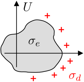
Refer to caption
Figure 3. Discrete and essential spectra defined in Theorem C.1.

We denote by $\mathcal{P}$ the analytic family of pseudo-differential equations $P_{\omega}$ (with $\omega\in{\mathbb{C}}$) on a closed manifold $X$ with degree$(P_{\omega})\equiv 0$ (we can always assume the last condition by using a left product with an invertible elliptic operator). The operators $P_{\omega}$ are continuous and linear from $L^{2}(X)$ into itself. The spectrum of this family is defined as the set of $\omega\in{\mathbb{C}}$ so that $P_{\omega}$ is not invertible. If $P_{\omega}$ is invertible, the inverse is also continuous. We also remind the reader that a pseudo-differential operator  $Q$ is elliptic at $(x,\boldsymbol{\xi})\in T^{\star}X\setminus 0$ if and only if the principal symbol $p(x,\boldsymbol{\xi})$ is invertible. $Q$ is elliptic if this holds for all $(x,\boldsymbol{\xi})\in T^{\star}X\setminus 0$. We will need the following theorem defining the different spectra (as illustrated in figure 3).

Theorem C.1.

Let $\mathcal{P}$ be as defined above, and $U\subset{\mathbb{C}}$ be the open set of the values of $\omega$ where $P_{\omega}$ is elliptic. Then, there exists a discrete subset $\sigma_{d}(\mathcal{P})$ of $U$ such that $P_{\omega}$ is not invertible. If $\omega\in\sigma_{d}(\mathcal{P})$, then $\dim(\ker(P_{\omega}))$ is finite. More precisely, for all $\omega\in U$, $P_{\omega}$ is Fredholm. If $\omega\in\sigma_{e}(\mathcal{P})={\mathbb{C}}\setminus U$, then $P_{\omega}$ is not invertible.

If $P_{\omega}$ is elliptic, we can define a right parametrix as

$$P_{\omega}R_{\omega}={\rm Id}+A_{\omega}$$

with $A_{\omega}$ smoothing and, similarly, a left parametrix $L_{\omega}$. Hence, $P_{\omega}$ is Fredholm and we can apply the Fredholm analytic theorem. Conversely, if $P_{\omega}$ is non-elliptic, it is non-invertible. We can use test functions of the form $a(x)e^{i\lambda x\boldsymbol{\xi}_{0}}$ with $p_{\omega}(a(x_{0}),\boldsymbol{\xi}_{0})=0$, where $p_{\omega}$ is the principal symbol of $P_{\omega}$, in order to show that the operator does not admit a continuous inverse (see [CdV20], section 2, for more details). This result also applies to the boundary calculus of pseudo-differential operator’s [BdM71, Gru08].

It follows from this that the essential spectrum of the Poincaré operator is the same, in the interval $0<\omega<\omega_{-}$, as the set of values of $\omega$ for which the Kelvin equation is invertible. Both properties are equivalent to say that the boundary symbol is non-elliptic. This depends on the symbolic calculus of boundary pseudo-differential operator’s, which is a rather technical issue. The identification of discrete spectra is much simpler. Indeed, we can transfer any eigenmodes of the Poincaré operator to a $H^{1}$ solution of the Kelvin equation (and conversely). More details will be given in future work, where we consider also the case of unstable stratification (i.e. $N^{2}<0$) for which a greater part of that calculation is needed.

References

  • [BdM71] Louis Boutet de Monvel. Boundary problems for pseudo-differential operators. Acta Math., 126:11–51, 1971.
  • [Car22] Élie Cartan. Sur les petites oscillations d’une masse fluide. Bull. Sci. Math., 46:317–369, 1922.
  • [CdV80] Yves Colin de Verdière. Spectre conjoint d’opérateurs pseudo-différentiels qui commutent. II. Le cas intégrable. Math. Z., 171:51–73, 1980.
  • [CdV20] Yves Colin de Verdière. Spectral theory of pseudodifferential operators of degree 0 and an application to forced linear waves. Anal. PDE, 13(5):1521–1537, 2020.
  • [CdVSR20] Yves Colin de Verdière and Laure Saint-Raymond. Attractors for two-dimensional waves with homogeneous Hamiltonians of degree 0. Commun. Pure Appl. Math., 73(2):421–462, 2020.
  • [CdVV23] Yves Colin de Verdière and Jérémie Vidal. The spectrum of the poincaré operator in an ellipsoid. arxiv:2305.01369, 2023.
  • [FS82a] Susan Friedlander and William L. Siegmann. Internal waves in a contained rotating stratified fluid. J. Fluid Mech., 114:123–156, 1982.
  • [FS82b] Susan Friedlander and William L. Siegmann. Internal waves in a rotating stratified fluid in an arbitrary gravitational field. Geophys. Astrophys. Fluid Dyn., 19(3-4):267–291, 1982.
  • [GKLP22] Alexandre Girouard, Mikhail Karpukhin, Michael Levitin, and Iosif Polterovich. The Dirichlet-to-Neumann map, the boundary Laplacian, and Hörmander’s rediscovered manuscript. J. Spectr. Theory, 12(1):195–225, 2022.
  • [Gru08] Gerd Grubb. Distributions and operators. Graduate Texts in Mathematics. Springer, 2008.
  • [Hö85] Lars Hörmander. The Analysis of Linear Partial Differential Operators III: Pseudo-differential operators. Springer-Verlag, 1985.
  • [Kel80] Lord Kelvin. On gravitational oscillations of rotating water. Proc. R. Soc. Edinburgh, 10:92–100, 1880.
  • [Poi85] Henri Poincaré. Sur l’équilibre d’une masse fluide animée d’un mouvement de rotation. Acta Math., 7:259–380, 1885.
  • [Tay13] Michael Taylor. Partial differential equations II: Qualitative studies of linear equations. Springer, 2013.
  • [VCdV24] Jérémie Vidal and Yves Colin de Verdière. Inertia-gravity waves in geophysical vortices. P. R. Soc. A, In press, 2024. https://doi.org/10.48550/arXiv.2402.10749.