Spectral Properties of Dual Complex Unit Gain Graphs

Abstract

In this paper, we study dual complex unit gain graphs and their spectral properties. We establish the interlacing theorem for dual complex unit gain graphs, and show that the spectral radius of a dual complex unit gain graph is always not greater than the spectral radius of the underlying graph, and these two radii are equal if and only if the dual complex unit gain graph is balanced. Similar results hold for the spectral radius of the Laplacian matrix of the dual complex unit gain graph too.

Key words. Unit gain graph, dual complex number, adjacency matrix, Laplacian matrix, eigenvalue.

1 Introduction

A gain graph assigns an element of a mathematical group to each of its edges, and if a group element is assigned to an edge, then the inverse of that group element is always assigned to the inverse edge of that edge [11, 14, 35]. In the literature, such a mathematical group usually consists of unit numbers of a number system. In this case, the gain graph is called a unit gain graph. The real unit gain graph is called a signed graph. The study of signed graphs is the forerunner of the study of unit gain graphs. It started in 2003 by Hou, Li and Pan [18] and was continued in [1, 3, 9, 10, 12, 13, 17, 39, 48]. In 2012, Reff [34] started the research on complex unit gain graphs. Since then, the study on complex unit gain graphs has grown explosively [2, 4, 5, 7, 8, 15, 16, 20, 21, 23, 24, 25, 26, 27, 36, 37, 38, 40, 42, 43, 44, 45, 46]. In 2022, Belardo, Brunettia, Coble, Reff and Skogman [6] studied quaternion unit gain graphs and their associated spectral theories, which were further studied in [19, 49]. The study of unit gain graphs and their spectral properties forms an important part of spectral graph theory.

In this paper, we study dual complex unit gain graphs and their spectral properties. In the literature, there are two different definitions of dual complex numbers. One is commutative in multiplication and can be regarded as a special case of dual quaternion numbers [28, 29, 41]. Such dual complex numbers found application in brain science [41]. In this paper, we consider such dual complex numbers. The other kind of dual complex numbers is noncommutative in multiplication, thus more complicated. See [29] for more explanations on these two kinds of dual complex numbers.

The study of dual complex unit gain graphs and their spectral properties will further enrich the theory of unit gain graphs, and the theory of dual complex numbers. It may also pave the way for studying dual quaternion unit gain graphs. Unit dual quaternions have wide applications in robotics research and computer graphics. In particular, it has applications in formation control of UAVs (unmanned aerial vehicles) and small satellites. Without knowing unit gain graphs, the relative configuration graphs studied in [33] are exactly dual quaternion unit gain graphs, and the dual quaternion Laplacian matrices proposed in [33] are exactly the Laplacian matrices in dual quaternion unit gain graphs. Also see [30]. It is worth exploring dual quaternion gain graphs later.

The remaining parts of this paper are distributed as follows. In the next section, we will review the knowledge of dual complex numbers and unit gain graphs. We study some basic properties of dual complex unit gain graphs in Section 3. In Section 4, we discuss the properties of eigenvalues of adjacency matrices of dual complex unit gain graphs. We establish the interlacing theorem for dual complex unit gain graphs, and show that the spectral radius of a dual complex unit gain graph is always not greater than the spectral radius of the underlying graph, and these two radii are equal if and only if the dual complex unit gain graph is balanced. Similar results hold for the spectral radius of the Laplacian matrix of the dual complex unit gain graph too. We state this in Section 5.

2 Dual Complex Numbers and Unit Gain Graphs

2.1 Dual complex numbers

A dual complex number $p=p_{s}+p_{d}\epsilon$ has standard part $p_{s}$ and dual part $p_{d}$. Both $p_{s}$ and $p_{d}$ are complex numbers. The symbol $\epsilon$ is the infinitesimal unit, satisfying $\epsilon^{2}=0$, and $\epsilon$ is commutative with complex numbers. If $p_{s}\not=0$, then we say that $p$ is appreciable. If $p_{s}$ and $p_{d}$ are real numbers, then $p$ is called a dual number. Denote the set of dual complex numbers by $\hat{\mathbb{C}}$.

The conjugate of $p=p_{s}+p_{d}\epsilon$ is $p^{*}=p_{s}^{*}+p_{d}^{*}\epsilon$, where $p_{s}^{*}$ and $p_{d}^{*}$ are the conjugates of the complex numbers $p_{s}$ and $p_{d}$, respectively. The real part of $p$ is defined by $Re(p)=Re(p_{s})+Re(p_{d})\epsilon$, where $Re(p_{s})$ and $Re(p_{d})$ are the real parts of the complex numbers $p_{s}$ and $p_{d}$, respectively. The standard part $p_{s}$ and the dual part $p_{d}$ of $p$ are also denoted by $St(p)$ and $Du(p)$, respectively.

Suppose we have two dual complex numbers $p=p_{s}+p_{d}\epsilon$ and $q=q_{s}+q_{d}\epsilon$. Then their sum is $p+q=(p_{s}+q_{s})+(p_{d}+q_{d})\epsilon$, and their product is $pq=p_{s}q_{s}+(p_{s}q_{d}+p_{d}q_{s})\epsilon$. The multiplication of dual complex numbers is commutative.

Suppose we have two dual numbers $p=p_{s}+p_{d}\epsilon$ and $q=q_{s}+q_{d}\epsilon$. By [31], if $p_{s}>q_{s}$, or $p_{s}=q_{s}$ and $p_{d}>q_{d}$, then we say $p>q$. Then this defines positive, nonnegative dual numbers, etc. If a dual number $p=p_{s}+p_{d}\epsilon$ is positive and appreciable, then

$$\sqrt{p}=\sqrt{p_{s}}+{p_{d}\over 2\sqrt{p_{s}}}\epsilon.$$

For a dual complex number $p=p_{s}+p_{d}\epsilon$, its squared norm is a nonnegative dual number

$$|p|^{2}=p^{*}p=p_{s}^{*}p_{s}+(p_{s}^{*}p_{d}+p_{d}^{*}p_{s})\epsilon,$$

and its magnitude is defined as a nonnegative dual number

$$|p|:=\left\{\begin{aligned} |p_{s}|+{(p_{s}p_{d}^{*}+p_{d}p_{s}^{*})\over 2|p_{s}|}\epsilon,&\ {\rm if}\ p_{s}\not=0,\\ |p_{d}|\epsilon,&\ {\rm otherwise}.\end{aligned}\right.$$ (1)

The dual complex number $p$ is invertible if and only if $p_{s}\neq 0$. Furthermore, if $p$ is invertible, there is $p^{-1}=\frac{p^{*}}{|p|^{2}}$.

Thus, a dual complex number $p=p_{s}+p_{d}\epsilon$ is a unit dual complex number if and only if $|p_{s}|=1$ and $p_{s}p_{d}^{*}+p_{d}p_{s}^{*}=0$. Equivalently, let $p_{s}=p_{s1}+p_{s2}i$ and $p_{d}=p_{d1}+p_{d2}i$. Then $p$ is a unit dual complex number if and only if $p_{s1}^{2}+p_{s2}^{2}=1$ and $p_{s1}p_{d1}+p_{s2}p_{d2}=0$. Furthermore, a unit dual complex number is always invertible and its inverse is its conjugate. Note that the product of two unit dual complex numbers is still a unit dual complex number. Hence, the set of unit dual complex numbers forms a group by multiplication.

Lemma 2.1.

Let $q_{1}$ and $q_{2}\in\hat{\mathbb{C}}$ be two dual complex numbers. Then

• $Re(q_{1})\leq|q_{1}|$ and the equality holds if and only if $q_{1}$ is a nonnegative dual number.

• $Re(q_{1})=Re({q^{*}_{1}})$ and $Re(q_{1}q_{2})=Re(q_{2}q_{1})$.

• $|q_{1}q_{2}|=|q_{1}||q_{2}|$.

• $|q_{1}+q_{2}|\leq|q_{1}|+|q_{2}|$.

An $n$-dimensional dual complex number vector is denoted by $\mathbf{x}=(x_{1},\cdots,x_{n})^{\top}$, where $x_{1},\dots,x_{n}$ are dual complex numbers. We may denote $\mathbf{x}=\mathbf{x}_{s}+\mathbf{x}_{d}\epsilon$, where $\mathbf{x}_{s}$ and $\mathbf{x}_{d}$ are two $n$-dimensional complex vectors. The $2$-norm of $\mathbf{x}$ is defined as

$$\|\mathbf{x}\|_{2}=\left\{\begin{array}[]{ll}\sqrt{\sum_{i=1}^{n}|x_{i}|^{2}},&\ \mathrm{if}\ \mathbf{x}_{s}\not=\mathbf{0},\\ \|\mathbf{x}_{d}\|_{2}\epsilon,&\ \mathrm{if}\ \mathbf{x}_{s}=\mathbf{0}.\end{array}\right.$$

If $\mathbf{x}_{s}\not=\mathbf{0}$, then we say that $\mathbf{x}$ is appreciable.

For an $n$-dimensional dual complex number vector $\mathbf{x}=(x_{1},\cdots,x_{n})^{\top}$, denote $\mathbf{x}^{*}=(x_{1}^{*},\cdots,x_{n}^{*})$. Let $\mathbf{y}=(y_{1},\cdots,y_{n})^{\top}$ be another $n$-dimensional dual complex number vectors. Define

$$\mathbf{x}^{*}\mathbf{y}=\sum_{j=1}^{n}x_{j}^{*}y_{j}.$$

If $\mathbf{x}^{*}\mathbf{y}=0$, we say that $\mathbf{x}$ and $\mathbf{y}$ are orthogonal. Note that $\mathbf{x}^{*}\mathbf{x}=\|\mathbf{x}\|_{2}^{2}$. Let $\mathbf{x}_{1},\cdots,\mathbf{x}_{n}$ be $n$ $n$-dimensional dual complex number vectors. If $\mathbf{x}_{i}^{*}\mathbf{x}_{j}=0$ for $i\not=j$ and $\mathbf{x}_{i}^{*}\mathbf{x}_{j}=1$ for $i=j$, $i,j=1,\cdots,n$, then we say that $\mathbf{x}_{1},\dots,\mathbf{x}_{n}$ form an orthonormal basis of the $n$-dimensional dual complex number vector space.

2.2 Dual complex matrices

Assume that $A=A_{s}+A_{d}\epsilon$ and $B=B_{s}+B_{d}\epsilon$ are two $n\times n$ dual complex matrices, where $n$ is a positive integer, $A_{s},A_{d},B_{s}$ and $B_{d}$ are four complex matrices, assume that $\lambda=\lambda_{s}+\lambda_{d}\epsilon$ and $\mu=\mu_{s}+\mu_{d}\epsilon$ are two dual complex numbers with $\lambda_{s},\lambda_{d},\mu_{s}$ and $\mu_{d}$ being complex numbers, and assume that $\mathbf{x}=\mathbf{x}_{s}+\mathbf{x}_{d}\epsilon$ and $\mathbf{y}=\mathbf{y}_{s}+\mathbf{y}_{d}\epsilon$ are two $n$-dimensional dual complex vectors with $\mathbf{x}_{s},\mathbf{x}_{d},\mathbf{y}_{s}$ and $\mathbf{y}_{d}$ being $n$-dimensional complex vectors.

If $AB=BA=I$, where $I$ is the $n\times n$ identity matrix, then we say that $B$ is the inverse of $A$ and denote that $B=A^{-1}$. We have the following proposition.

Proposition 2.2.

Suppose that $A=A_{s}+A_{d}\epsilon$ and $B=B_{s}+B_{d}\epsilon$ are two $n\times n$ dual complex matrices, where $n$ is a positive integer, $A_{s},A_{d},B_{s}$ and $B_{d}$ are four complex matrices. Then the following four statements are equivalent.

(a) $B=A^{-1}$;

(b) $AB=I$;

(c) $A_{s}B_{s}=I$ and $A_{s}B_{d}+A_{d}B_{s}=O$, where $O$ is the $n\times n$ zero matrix;

(d) $B_{s}=A_{s}^{-1}$ and $B_{d}=-A_{s}^{-1}A_{d}A_{s}^{-1}$.

If there is an $n\times n$ invertible dual complex matrix $P$ such that $A=P^{-1}BP$, then we say that $A$ and $B$ are similar, and denote $A\sim B$.

For an $n\times n$ dual complex matrix $A$, denote its conjugate transpose as $A^{*}$. If $A^{*}=A^{-1}$, then $A$ is called a unitary matrix. If a dual number matrix is a unitary matrix, then we simply call it an orthogonal matrix. Let $A\in\hat{\mathbb{C}}^{n\times m}$. Then the null space generated by $A$ is

$$\text{null}(A)=\{{\mathbf{x}}\,|\,A^{*}{\mathbf{x}}=0\},$$

and the span of $A$ is

$$\text{span}(A)=\{{\mathbf{x}}\,|\,\exists{\mathbf{y}}\in\hat{\mathbb{C}}^{m}\text{ such that }{\mathbf{x}}=A{\mathbf{y}}\}.$$

Proposition 2.3.

Let $U=[\mathbf{u}_{1},\cdots,\mathbf{u}_{n}]\in\hat{\mathbb{C}}^{n\times n}$ such that its columns form an orthonormal basis in $\hat{\mathbb{C}}^{n}$. Then ${U^{*}U}=I$ and the following results hold.

(i) For any vector ${\mathbf{x}}\in\hat{\mathbb{C}}^{n}$, there exists ${\mathbf{y}}\in\hat{\mathbb{C}}^{n}$ such that $\mathbf{x}=U\mathbf{y}$.

(ii) Suppose that $1<k<n$ and $U=[U_{1},U_{2}]$, where ${U}_{1}\in\hat{\mathbb{C}}^{n\times k}$ and ${U}_{2}\in\hat{\mathbb{C}}^{n\times(n-k)}$. Then $\text{null}({U}_{1})=\text{span}({U}_{2})$.

Proof.

(i) Let $U=U_{s}+U_{d}\epsilon$, $\mathbf{x}=\mathbf{x}_{s}+\mathbf{x}_{d}\epsilon$. Since $U_{s}^{*}U_{s}=I$, the rank of $\begin{bmatrix}U_{s}&O\\ U_{d}&U_{s}\end{bmatrix}$ is equal to $2n$. Therefore,

$$\begin{bmatrix}U_{s}&O\\ U_{d}&U_{s}\end{bmatrix}\begin{bmatrix}{\mathbf{y}}_{s}\\ {\mathbf{y}}_{d}\end{bmatrix}=\begin{bmatrix}{\mathbf{x}}_{s}\\ {\mathbf{x}}_{d}\end{bmatrix}$$

always has a solution $\mathbf{y}=\mathbf{y}_{s}+\mathbf{y}_{d}\epsilon$ for any ${\mathbf{x}}_{s}$ and ${\mathbf{x}}_{d}$.

(ii) By ${U^{*}U}=I$, we have ${U_{1}^{*}U_{2}}=O_{k\times(n-k)}$, the $k\times(n-k)$ zero matrix. Let $\mathbf{x}=U\mathbf{y}=U_{1}\mathbf{y}_{1}+U_{2}\mathbf{y}_{2}$. On one hand, if $\mathbf{x}\in\text{null}(U_{1})$, then $U_{1}^{*}\mathbf{x}=\mathbf{y}_{1}={\mathbf{0}}$. Thus $\text{null}({U}_{1})\subseteq\text{span}({U}_{2})$. On the other hand, if ${\mathbf{x}}\in\text{span}({U}_{2})$, then $\mathbf{x}=U_{2}\mathbf{y}_{2}$. Thus, ${U_{1}^{*}\mathbf{x}={\mathbf{0}}}$ and $\text{span}({U}_{2})\subseteq\text{null}({U}_{1})$.

This completes the proof. ∎

If

$$A\mathbf{x}=\lambda\mathbf{x},$$ (2)

where $\mathbf{x}$ is appreciable, i.e., $\mathbf{x}_{s}\not=\mathbf{0}$, then $\lambda$ is called an eigenvalue of $A$, with an eigenvector $\mathbf{x}$.

By definition, if $A\sim B$, then $A$ and $B$ have the same eigenvalue set. We have the following proposition.

Proposition 2.4.

Suppose that $A$ and $B$ are two $n\times n$ dual complex matrices, $A\sim B$, i.e., $A=P^{-1}BP$ for some $n\times n$ invertible dual complex matrix $P$, and $\lambda$ is a dual complex eigenvalue of $A$ with a dual complex eigenvector $\mathbf{x}$. Then $\lambda$ is an eigenvalue of $B$ with an eigenvector $P\mathbf{x}$.

Since $A=A_{s}+A_{d}\epsilon$, $\lambda=\lambda_{s}+\lambda_{d}\epsilon$ and $\mathbf{x}=\mathbf{x}_{s}+\mathbf{x}_{d}\epsilon$, (2) is equivalent to

$$A_{s}\mathbf{x}_{s}=\lambda_{s}\mathbf{x}_{s},$$ (3)

with $\mathbf{x}_{s}\not=\mathbf{0}$, i.e., $\lambda_{s}$ is an eigenvalue of $A_{s}$ with an eigenvector $\mathbf{x}_{s}$, and

$$(A_{s}-\lambda_{s}I)\mathbf{x}_{d}-\lambda_{d}\mathbf{x}_{s}=-A_{d}\mathbf{x}_{s}.$$ (4)

Following [32], we may prove that if $A$ is Hermitian, then it has exactly $n$ dual number eigenvalues, with orthonormal eigenvectors, and $A$ is positive semidefinite (definite) if and only if its eigenvalues are nonnegative (positive).

By [29], a non-Hermitian dual number matrix may have no eigenvalue at all, or have infinitely many eigenvalues. The following proposition can be found in [29].

Proposition 2.5.

Suppose that $A$ is an $n\times n$ dual complex diagonalizable matrix, i.e., $A$ is similar to a dual complex diagonal matrix. Then $A$ has exactly $n$ eigenvalues.

An $n\times n$ dual complex Hermitian matrix $A$ is always diagonalizable in the sense that $A=P{\Sigma}P^{-1}$, where ${\Sigma}$ is an $n\times n$ dual number diagonal matrix, while $P$ is a dual complex unitary matrix.

For more knowledge of dual complex matrices, please see [28, 29, 31, 41].

2.3 Unit gain graphs

Suppose $G=(V,E)$ is a graph, where $V:=\{v_{1},v_{2},\cdots,v_{n}\}$ and $E=\{e_{ij}\}$. Define $n:=|V|$ and $m:=|E|$. The degree of a vertex $v_{j}$ is denoted by $d_{j}=\text{deg}(v_{j})$ and the maximum degree is $\Delta=\max d_{j}$. An oriented edge from $v_{i}$ to $v_{j}$ is denoted by $e_{ij}$. The set of oriented edges, denoted by $\vec{E}(G)$, contains two copies of each edge with opposite directions. Then $\left|\vec{E}\right|=2m$. Even though $e_{ij}$ stands for an edge and an oriented edge simultaneously, it will always be clear in the content. By graph theory, $G$ is bidirectional.

A gain graph is a triple $\Phi=(G,\Omega,\varphi)$ consisting of an underlying graph $G=(V,E)$, the gain group $\Omega$ and the gain function $\varphi:\vec{E}(G)\rightarrow\Omega$ such that $\varphi(e_{ij})=\varphi^{-1}(e_{ji})$. The gain group may be the set of complex units, the set of unit quaternion numbers, or the set of unit dual complex numbers, etc. In this paper, we will focus on the dual complex unit gain graphs, denoted by $\hat{\mathbb{T}}$-gain graphs. If there is no confusion, then we simply denote the gain graph as $\Phi=(G,\varphi)$.

A switching function is a function $\zeta:V\rightarrow\Omega$ that switches the $\Omega$-gain graph $\Phi=(G,\varphi)$ to $\Phi^{\zeta}=(G,\varphi^{\zeta})$, where

$$\varphi^{\zeta}(e_{ij})=\zeta^{-1}(v_{i})\varphi(e_{ij})\zeta(v_{j}).$$

In this case, $\Phi$ and $\Phi^{\zeta}$ are switching equivalent, denoted by $\Phi\sim\Phi^{\zeta}$. Further, denote the switching class of $\varphi$ as $[\Phi]$, which is the set of gain graphs switching equivalent to $\Phi$.

The gain of a walk $W=v_{1}e_{12}v_{2}e_{23}v_{3}\cdots v_{k-1}e_{k-1,k}v_{k}$ is

$$\varphi(W)=\varphi(e_{12})\varphi(e_{23})\cdots\varphi(e_{k-1,k}).$$ (5)

A walk $W$ is neutral if $\varphi(W)=1_{\Omega}$, where $1_{\Omega}$ is the identity of $\Omega$. An edge set $S\subseteq E$ is balanced if every cycle $C\subseteq S$ is neutral. A subgraph is balanced if its edge set is balanced.

Let $\Phi=(G,\Omega,\varphi)$ be a gain graph and $A(\Phi)=(a_{ij}(\Phi))$ and $L(\Phi)$ be the adjacency and Laplacian matrices of $\Phi$, respectively. Define $A(\Phi)$ and $L(\Phi)$ via the gain function $\varphi(e)$ as follows,

$$a_{ij}{(\Phi)}=\left\{\begin{array}[]{cl}\varphi(e_{ij}),&\text{if }e_{ij}\in{E(\Phi)},\\ 0,&\text{otherwise},\end{array}\right.\ \text{ and }L(\Phi)=D(\Phi)-A(\Phi).$$ (6)

Here, $\varphi(e_{ij})\in\hat{\mathbb{T}}$, $\varphi(e_{ij})=\varphi(e_{ji})^{-1}=\overline{\varphi(e_{ji})}$, and $D(\Phi)$ is an $n\times n$ diagonal matrix with each diagonal element being the degree of the corresponding vertex in its underlying graph $G$.

Denote by $-\Phi$ the gain graph $(G,\Omega,-\varphi)$ obtained by replacing the gain of each edge with its opposite. Clearly, $A(-\Phi)=-A(\Phi)$. Furthermore, $\Phi$ is antibalanced if and only if $-\Phi$ is balanced.

The potential function is a function $\theta:V\rightarrow\Omega$ such that for every $e_{ij}\in{E(\Phi)}$,

$$\varphi(e_{ij})=\theta(v_{i})^{-1}\theta(v_{j}).$$ (7)

We write $(G,1_{\Omega})$ as the $\Omega$-gain graph with all neutral edges. Note $\theta$ is not unique since for any invertible variable $q\in\Omega$, $\tilde{\theta}(v_{i})=q\theta(v_{i})$ for all $v_{i}\in V$ is also a potential function of $\Phi$.

The following result can be deduced from [47]. Also see [6].

Lemma 2.6.

Let $\Phi=(G,\Omega,\varphi)$ be a gain graph. Then the following are equivalent:

• $\Phi$ is balanced.

• $\Phi\sim(G,1_{\Omega})$.

• $\varphi$ has a potential function.

3 Dual Complex Unit Gain Graphs

Let $\Phi=(G,\hat{\mathbb{T}},\varphi)$ be a dual complex unit gain graph. In the following, we simply denote the adjacency and Laplacian matrices as $A$ and $L$, respectively.

By Lemma 2.6, we have the following lemma for dual complex unit gain graphs.

Lemma 3.1.

Let $\Phi=(G,\hat{\mathbb{T}},\varphi)$ be a dual complex unit gain graph. Then the following are equivalent:

• $\Phi$ is balanced.

• $\Phi\sim(G,1_{\hat{\mathbb{T}}})$.

• $\varphi$ has a potential function.

Let $\Phi=(G,\hat{\mathbb{T}},\varphi)$ be a dual complex unit gain graph with $n$ vertices. Then the adjacency matrix $A(\Phi)$ and the Laplacian matrix $L(\Phi)$ are two $n\times n$ dual complex Hermitian matrices. Thus, each of $A(\Phi)$ and $L(\Phi)$ has $n$ eigenvalues. The set of the $n$ eigenvalues of $A(\Phi)$ is called the spectrum of $\Phi$, and denoted as $\sigma_{A}(\Phi)$, while the set of the $n$ eigenvalues of $L(\Phi)$ is called the Laplacian spectrum of $\Phi$, and denoted as $\sigma_{L}(\Phi)$. We also denote the eigenvalue sets of the adjacency and Laplacian matrices of the underlying graph $G$ as $\sigma_{A}(G)$ and $\sigma_{L}(G)$, respectively. We have the following theorem.

Theorem 3.2.

Let $\Phi=(G,\hat{\mathbb{T}},\varphi)$ be a dual complex unit gain graph with $n$ vertices. If $\Phi$ is balanced, then its spectrum $\sigma_{A}(\Phi)$ consists of $n$ real numbers, while its Laplacian spectrum $\sigma_{L}(\Phi)$ consists of one zero and $n-1$ positive numbers. Furthermore, we have $\sigma_{A}(\Phi)=\sigma_{A}(G)$ and $\sigma_{L}(\Phi)=\sigma_{L}(G)$.

Proof.

By Lemma 3.1, we have $\Phi\sim\Phi^{1}:=(G,1_{\hat{\mathbb{T}}})$. Then $\Phi^{1}$ is exactly the underlying graph $G$, and the adjacency and the Laplacian matrices of $\Phi^{1}$ are the adjacency and Laplacian matrices of $G$, respectively. It follows from $\Phi\sim\Phi^{1}$ that there exists a function $\zeta$ such that for all $e_{ij}\in\color[rgb]{0,0,0}E(\Phi)$, there is

$$\zeta^{-1}(v_{i})\varphi(e_{ij})\zeta(v_{j})=1.$$

Thus, we have

$$A(\Phi^{1})=Z^{-1}A(\Phi)Z,\text{ where }Z=\text{diag}(\zeta(v_{1}),\cdots,\zeta(v_{n})),$$

and $L(\Phi^{1})={D(\Phi^{1})}-A(\Phi^{1})=Z^{-1}({D(\Phi)}-A(\Phi))Z=Z^{-1}L(\Phi)Z$. In other words, $A(\Phi^{1})$ and $L(\Phi^{1})$ are similar with $A(\Phi)$ and $L(\Phi)$, respectively. Now, the conclusions of this theorem follow from the spectral properties of adjacency and Laplacian matrices of ordinary graphs. ∎

If $G$ is a tree, then $\Phi$ is balanced, and the eigenvalues of the adjacency and the Laplacian matrices of $\Phi$ are the same with those of the adjacency and Laplacian matrices of $G$, respectively. For instance, a path is a special tree. Let $P_{n}$ be the path graph on $n$ vertices and $\Phi=(P_{n},\hat{\mathbb{T}},\varphi$). Then the eigenvalues of $A(\Phi)$ and $L(\Phi)$ can be calculated as

$$\sigma_{A}(\Phi)=\left\{2\cos\left(\frac{\pi j}{n+1}\right):\ j\in\{1,\dots,n\}\right\},$$

and

$$\sigma_{L}(\Phi)=\left\{2-2\cos\left(\frac{\pi j}{n}\right):\ j\in\{0,\dots,n-1\}\right\}.$$

If $\Phi$ is not balanced, then the eigenvalues of $A(\Phi)$ may not be real numbers. The following example illustrates this.

(a) $\hat{\mathbb{T}}$-gain graph $\Phi_{1}$

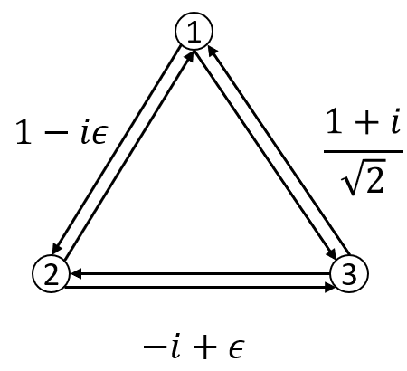
(b) $\hat{\mathbb{T}}$-gain graph $\Phi_{2}$

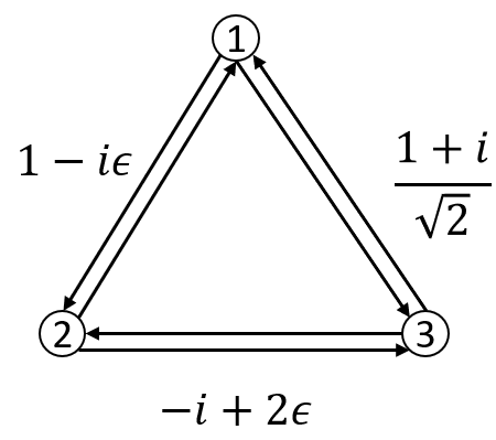
(c) $\hat{\mathbb{T}}$-gain graph $\Phi_{3}$

Figure 1: Three $\hat{\mathbb{T}}$-gain graphs

Example 3.3.

Consider three $\hat{\mathbb{T}}$-gain cycles in Figure 1. Their adjacency matrices are given as follows.

$$A(\Phi_{1})=\begin{bmatrix}0&1-i\epsilon&-i\\ 1+i\epsilon&0&-i+\epsilon\\ i&i+\epsilon&0\end{bmatrix},\quad A(\Phi_{2})=\begin{bmatrix}0&1-i\epsilon&{\frac{1-i}{\sqrt{2}}}\\ 1+i\epsilon&0&-i+\epsilon\\ \frac{1+i}{\sqrt{2}}&i+\epsilon&0\end{bmatrix},$$

and

$$A(\Phi_{3})=\begin{bmatrix}0&1-i\epsilon&{\frac{1-i}{\sqrt{2}}}\\ 1+i\epsilon&0&-i+2\epsilon\\ \frac{1+i}{\sqrt{2}}&i+2\epsilon&0\end{bmatrix},$$

respectively. The $\hat{\mathbb{T}}$-gain graph $\Phi_{1}$ is balanced, and the eigenvalues of its adjacency matrix are

$$\sigma_{A}(\Phi_{1})=\{2,\quad-1,\quad-1\},$$

which are the same with the eigenvalues of the adjacency matrix of its underlying graph. The eigenvalues of $A(\Phi_{2})$ are all real numbers, i.e.,

$$\sigma_{A}(\Phi_{2})=\{1.9319,\quad-0.5176,\quad-1.4142\}.$$

The eigenvalues of $A(\Phi_{3})$ are all dual numbers, i.e.,

$$\sigma_{A}(\Phi_{3})=\{1.9319+{0.1725}\epsilon,\quad-0.5176{-0.6440}\epsilon,\quad-1.4142{+0.4714}\epsilon\},$$

and the standard parts of $\sigma_{A}(\Phi_{3})$ are the same with $\sigma_{A}(\Phi_{2})$.

The closed form of the adjacency and Laplacian eigenvalues of a cycle $\mathbb{T}$-gain graph is presented in Theorem 5.1 in [34]. Let $C_{n}$ be the cycle on $n$ vertices and $\Phi=(C_{n},\mathbb{T},\varphi$). Suppose $\varphi(C_{n})=e^{i\theta}\in\mathbb{T}$. Then the eigenvalues of $A(\Phi)$ and $L(\Phi)$ can be calculated as

$$\sigma_{A}(\Phi)=\left\{2\cos\left(\frac{\theta+2\pi j}{n}\right):\ j\in\{0,\dots,n-1\}\right\},$$ (8)

and

$$\sigma_{L}(\Phi)=\left\{2-2\cos\left(\frac{\theta+2\pi j}{n}\right):\ j\in\{0,\dots,n-1\}\right\},$$ (9)

respectively. We now study $\hat{\mathbb{T}}$-gain graphs.

Proposition 3.4.

Let $C_{n}:=v_{1}e_{12}v_{2}\dots v_{n}e_{n1}v_{1}$ be the cycle on $n$ vertices and $\Phi=(C_{n},\hat{\mathbb{T}},\varphi$). Suppose $\varphi(C_{n})=e^{i\theta}+q_{d}\epsilon\in\hat{\mathbb{T}}$. Then the following results hold.

(i) There exists a switching function $\zeta:V(\Phi)\rightarrow\hat{\mathbb{T}}$ such that $\varphi^{\zeta}(e_{i,i+1})=1$ for $i=1,\dots,n-1$ and $\varphi^{\zeta}(e_{n,1})=\varphi(C_{n})$.

(ii) If $q_{d}=0$, then the eigenvalues of $A(\Phi)$ and $L(\Phi)$ can be calculated by equations (8) and (9), respectively.

(iii) If $q_{d}\neq 0$, then

$$St(\sigma_{A}(\Phi))=\left\{2\cos\left(\frac{\theta+2\pi j}{n}\right):\ j\in\{0,\dots,n-1\}\right\},$$

and

$$St(\sigma_{L}(\Phi))=\left\{2-2\cos\left(\frac{\theta+2\pi j}{n}\right):\ j\in\{0,\dots,n-1\}\right\}.$$

Proof.

(i) Define the switching function $\zeta:V(\Phi)\rightarrow\hat{\mathbb{T}}$ as follows:

$$\zeta(v_{i})=\left\{\begin{array}[]{ll}1,&i=1,\\ \left(\Pi_{j=1}^{i-1}\varphi(e_{j,j+1})\right)^{-1},&i=2,\cdots,n.\end{array}\right.$$

Then for $i=1$, there is

$$\varphi^{\zeta}(e_{12})=\zeta(v_{1})^{-1}\varphi(e_{12})\zeta(v_{2})=\varphi(e_{12})\varphi(e_{12})^{-1}=1.$$

For $i=2,\dots,n-1$, there is

$$\varphi^{\zeta}(e_{i,i+1}) = \zeta(v_{i})^{-1}\varphi(e_{i,i+1})\zeta(v_{i+1})$$

$$= \Pi_{j=1}^{i-1}\varphi(e_{j,j+1})\varphi(e_{i,i+1})\left(\Pi_{j=1}^{i}\varphi(e_{j,j+1})\right)^{-1}$$

$$= 1.$$

For $i=n$, there is

$$\varphi^{\zeta}(e_{n,1}) = \zeta(v_{n})^{-1}\varphi(e_{n,1})\zeta(v_{1})=\Pi_{j=1}^{n-1}\varphi(e_{j,j+1})\varphi(e_{n,1})=\varphi(C_{n}).$$

(ii) If $q_{d}=0$, then $\Phi^{\zeta}$ is a $\mathbb{T}$-gain graph, whose adjacency and Laplacian eigenvalues can be computed by (8) and (9), respectively. This conclusion follows directly from the fact that $\Phi$ and $\Phi^{\zeta}$ have the same adjacency and Laplacian eigenvalues.

(iii) If $q_{d}\neq 0$, both $A(\Phi)$ and $L(\Phi)$ are dual complex matrices, and their standard parts $St(A(\Phi))$ and $St(L(\Phi))$ are adjacency and Laplacian matrices of the $\mathbb{T}$-gain graph $\Phi_{s}=(G,\mathbb{T},St(\varphi))$, respectively. For a dual complex matrix, the standard parts of the eigenvalues are corresponding to the eigenvalues of the standard parts of this dual complex matrix [32]. Therefore, we get the desired results.

This completes the proof. ∎

4 Eigenvalues of Adjacency Matrices

The switching class has a unique adjacency spectrum.

Proposition 4.1.

Let $\Phi_{1}=(G,\varphi_{1})$ and $\Phi_{2}=(G,\varphi_{2})$ be both $\hat{\mathbb{T}}$-gain graphs. If $\Phi_{1}\sim\Phi_{2}$, then $\Phi_{1}$ and $\Phi_{2}$ have the same spectrum. That is, $\sigma_{A}(\Phi_{1})=\sigma_{A}(\Phi_{2})$.

Let $\Phi=(G,\varphi)$ be a $\hat{\mathbb{T}}$-gain graph, and $S$ be a subset of $V$. Denote $\Phi[S]$ as the induced subgraph of $\Phi$ with vertex set $S$, and $\Phi-S$ as $\Phi[V\setminus S]$, respectively. Both the adjacency matrices $A(\Phi)$ and $A(\Phi[S])$ are Hermitian matrices. As stated in Section 2, an $n\times n$ dual complex Hermitian matrix has exactly $n$ eigenvalues, which are dual numbers. The following theorem shows the eigenvalues of $A(\Phi)$ interlace with those of $A(\Phi[S])$.

Theorem 4.2.

(Interlacing Theorem) Let $\Phi=(G,\varphi)$ be a $\hat{\mathbb{T}}$-gain graph with $n$ vertices and $S$ be a subset of $V$ with $k$ vertices. Denote the eigenvalues of $A(\Phi)$ and $A(\Phi[S])$ by

$${\lambda_{1}\geq\lambda_{2}\cdots\geq\lambda_{n}\quad\text{and}\quad\mu_{1}\geq\mu_{2}\geq\cdots\geq\mu_{k},}$$

respectively. Then the following inequalities hold:

$$\lambda_{i}\geq\mu_{i}\geq\lambda_{n+i-k},\quad\forall\,1\leq i\leq k.$$ (10)

Proof.

Suppose some basis eigenvectors of $A(\Phi)$ and $A(\Phi[S])$ are $\{\mathbf{x}_{1},\dots,\mathbf{x}_{n}\}$ and $\{\mathbf{y}_{1},\dots,\mathbf{y}_{k}\}$, respectively. Without loss of generality, assume

$$A(\Phi)=\left[\begin{array}[]{cc}A(\Phi[S])&X^{*}\\ X&Z\end{array}\right].$$

For $1\leq i\leq k$, define the following vector spaces

$$U=\text{span}(\mathbf{x}_{i},\dots,\mathbf{x}_{n}),\ V=\text{span}(\mathbf{y}_{1},\dots,\mathbf{y}_{i}),\ W=\left\{\left(\begin{array}[]{c}{\mathbf{y}}\\ 0\end{array}\right)\in\hat{\mathbb{C}}^{n},{\mathbf{y}}\in V\right\}.$$

By Theorem 4.4 in [22] and Proposition 2.3 (ii), we have

$$\lambda_{i}=\max_{\mathbf{x}\in U}\ \|\mathbf{x}\|^{-2}(\mathbf{x}^{*}A(\Phi)\mathbf{x})\quad\text{and}\quad\mu_{i}=\min_{\mathbf{x}\in V}\ \|\mathbf{x}\|^{-2}(\mathbf{x}^{*}A(\Phi[S])\mathbf{x}).$$

Furthermore, the following system

$$\begin{bmatrix}U_{s}&O&-W_{s}&O\\ U_{s}&U_{d}&-W_{s}&-W_{d}\end{bmatrix}\begin{bmatrix}{\mathbf{v}}_{s}\\ {\mathbf{v}}_{d}\\ {\mathbf{z}}_{s}\\ {\mathbf{z}}_{d}\end{bmatrix}=\begin{bmatrix}O\\ O\end{bmatrix}$$

always has solutions since the size of its coefficient matrix is $2n\times(2n+2)$. Let $\mathbf{v}=\mathbf{v}_{s}+\mathbf{v}_{d}\epsilon$ and $\mathbf{z}=\mathbf{z}_{s}+\mathbf{z}_{d}\epsilon$. Then, there exists $\mathbf{w}=U{\mathbf{v}}=W{\mathbf{z}}\in U\cap W$. Suppose that $\mathbf{w}=\begin{pmatrix}{\mathbf{y}}\\ 0\end{pmatrix}$. Then we derive that

$$\lambda_{i}\geq\|\mathbf{w}\|^{-2}(\mathbf{w}^{*}A(\Phi)\mathbf{w})=\|{\mathbf{y}}\|^{-2}\left({\mathbf{y}}^{*}A(\Phi[S]){\mathbf{y}}\right)\geq\mu_{i}.$$

This proves the first part in (10).

The second inequality in (10) can be derived by choosing

$$U=\text{span}(\mathbf{x}_{1},\dots,\mathbf{x}_{n+i-k}),\ V=\text{span}(\mathbf{y}_{i},\dots,\mathbf{y}_{k}),\ W=\left\{\left(\begin{array}[]{c}v\\ 0\end{array}\right)\in\hat{\mathbb{C}}^{n},v\in V\right\},$$

and we do not repeat the details here. ∎

Corollary 4.3.

Let $\Phi=(G,\varphi)$ be a $\hat{\mathbb{T}}$-gain graph with $n$ vertices. For any vertex $v\in V$, the eigenvalues of $A(\Phi)$ and of $A(\Phi-v)$ labeled in decreasing order interlace as follows.

$$\lambda_{1}(\Phi)\geq\lambda_{1}(\Phi-v)\geq\lambda_{2}(\Phi)\geq\lambda_{2}(\Phi-v)\geq\cdots\geq\lambda_{n-1}(\Phi-v)\geq\lambda_{n}(\Phi).$$

The following proposition presents some results for the eigenvalues and eigenvectors of the adjacency matrix of a dual complex unit gain graph.

Proposition 4.4.

Let $\Phi=(G,\varphi)$ be a $\hat{\mathbb{T}}$-gain graph with $n$ vertices and $A=A(\Phi)$ be the adjacency matrix. Suppose $\lambda=\lambda_{s}+\lambda_{d}\epsilon$ is an eigenvalue of $A$ and $\mathbf{x}={\mathbf{x}}_{s}+{\mathbf{x}}_{d}\epsilon=(x_{1},\cdots,x_{n})^{\top}$ is its corresponding unit eigenvector. Then the following results hold.

• The eigenvalue satisfies

  $$\lambda=\mathbf{x}^{*}A\mathbf{x}=\sum_{e_{ij}\in E(\Phi)}2Re({x_{i}^{*}}\varphi(e_{ij})x_{j}).$$

• $\lambda_{s}$ is an eigenvalue of the complex matrix $A_{s}$ with an eigenvector ${\mathbf{x}}_{s}$.

• The dual part satisfies $\lambda_{d}={\mathbf{x}}_{s}^{*}A_{d}{\mathbf{x}}_{s}$. Furthermore, if $A_{s}$ has $n$ simple eigenvalues $\lambda_{s,i}$ with associated unit eigenvectors $x_{s,i}$’s. Then $A$ has exactly $n$ eigenvalues $\lambda_{i}=\lambda_{s,i}+\lambda_{d,i}\epsilon$ with associated eigenvectors ${\mathbf{x}}_{i}={\mathbf{x}}_{s,i}+{\mathbf{x}}_{d,i}\epsilon$, $i=1,\cdots,n$, where

  $$\lambda_{d}={\mathbf{x}}_{s}^{*}A_{d}{\mathbf{x}}_{s}\ \text{and}\ {\mathbf{x}}_{d,i}=\sum_{j\neq i}\frac{{\mathbf{x}}_{s,j}{\mathbf{x}}_{s,j}^{*}(A_{d}-\lambda_{d,i}I_{n}){\mathbf{x}}_{s,i}}{\lambda_{s,i}-\lambda_{s,j}}.$$

• Two eigenvectors of $A$, associated with two eigenvalues with distinct standard parts, are orthogonal to each other.

These results follow directly from [32] and we omit the details of their proofs here.

In general, the spectral radius of a dual complex matrix is not well defined since a dual complex matrix may have no eigenvalue at all or have infinitely many eigenvalues. When the dual complex matrix is Hermitian, all of its eigenvalues are dual numbers and we are able to define their order by [31]. Here, let $\rho_{A}(G)$ be the adjacency spectral radius of the underlying graph $G$ and $\rho_{A}(\Phi)$ be the adjacency spectral radius of the unit gain graph $\Phi$, respectively. The following theorem generalizes that of signed graphs [11, 39] and complex unit gain graphs [27].

Theorem 4.5.

Let $\Phi=(G,\varphi)$ be a $\hat{\mathbb{T}}$-gain graph. Then

$$\rho_{A}(\Phi)\leq\rho_{A}(G).$$ (11)

Furthermore, if $\Phi$ is connected, then ${\lambda_{1}}(\Phi)=\rho_{A}(G)$ (resp. $-\lambda_{n}(\Phi)=\rho_{A}(G)$) if and only if $\Phi$ is balanced (resp. antibalanced). Here, $\lambda_{1}(\Phi)$ and $\lambda_{n}(\Phi)$ are the largest and the smallest eigenvalues of $A(\Phi)$, respectively.

Proof.

Denote $A=A(G)$, and $B=(B_{ij})=A(\Phi)=B_{s}+B_{d}\epsilon$ with $B_{ij}={B_{ijs}+B_{ijd}\epsilon=}\varphi(e_{ij})$. Suppose $\mathbf{x}\in{\hat{\mathbb{C}}}^{n}$ is a unit eigenvector of $B$ corresponding to an eigenvalue $\lambda$ of $B=A(\Phi)$. Let ${\bf y}=|\mathbf{x}|$. Then we have

$$|\lambda| = |\mathbf{x}^{*}{B}\mathbf{x}|$$

$$= 2{\left|\sum_{{e_{ij}}\in E(\Phi)}Re({x_{i}^{*}}\varphi(e_{ij})x_{j})\right|}$$

$$\leq 2\sum_{{e_{ij}}\in E(\Phi)}|{x_{i}^{*}}\varphi(e_{ij})x_{j}|$$

$$= 2\sum_{{e_{ij}}\in E(\Phi)}|{x_{i}^{*}}||\varphi(e_{ij})||x_{j}|$$

$$= 2\sum_{{e_{ij}}\in E(\Phi)}|{x_{i}^{*}}||x_{j}|$$

$$= {\bf y}^{*}A(G){\bf y},$$

where the first and the second equalities follow from Proposition 4.4 (i), the first inequality and the third equality follow from Lemma 2.1, the fourth equality follows from $\varphi(e_{ij})\in\hat{\mathbb{T}}$ for any ${e_{ij}}\in\color[rgb]{0,0,0}E(\Phi)$. Therefore,

$$St(|\lambda|)\leq St({\bf y}^{*}A(G){\bf y})\leq\rho_{A}(G).$$

If $St(|{\lambda}|)<\rho_{A}(G)$ for any eigenvalue $\lambda$ of $B$, then $\rho_{A}(\Phi)<\rho_{A}(G)$. Otherwise, if there exists an eigenvalue $\lambda$ of $B=A(\Phi)$ satisfying $St(|{\lambda|})=St({\bf y}^{*}A(G){\bf y})=\rho_{A}(G)$, we claim that ${\lambda_{d}}=0$.

By Proposition 4.4, we have

$${\lambda_{d}}=\mathbf{x}_{s}^{*}B_{d}\mathbf{x}_{s}=\sum_{{e_{ij}}\in E(\Phi)}x_{is}^{*}B_{ijd}x_{js}=\sum_{{e_{ij}}\in E(\Phi)\cap\mathcal{A}_{x}}x_{is}^{*}B_{ijd}x_{js},$$

where $\mathcal{A}_{x}=\{{e_{ij}}\,|\,x_{is}\neq 0,\ x_{js}\neq 0\}$. Since $St(|{\lambda}|)=St({\bf y}^{*}A(G){\bf y})$, the equality of the standard part holds true in (4). Therefore, for all ${e_{ij}}\in E(\Phi)\cap\mathcal{A}_{x}$, we have

$$B_{ijs}=\frac{x_{is}}{|x_{is}|}\frac{x_{js}^{*}}{|x_{js}|}.$$

Since each element in $B$ is a unit dual complex number, there is $B_{ijs}^{*}B_{ijd}+B_{ijd}^{*}B_{ijs}=0$ for all ${e_{ij}}\in E(\Phi)$. Therefore,

$${\lambda_{d}} = \sum_{{e_{ij}}\in E(\Phi)\cap\mathcal{A}_{x}}x_{is}^{*}B_{ijd}x_{js}$$

$$= \sum_{{e_{ij}}\in E(\Phi)\cap\mathcal{A}_{x}}B_{ijd}B_{ijs}^{*}|x_{is}||x_{js}|$$

$$= \frac{1}{2}\sum_{{e_{ij}}\in E(\Phi)\cap\mathcal{A}_{x}}(B_{ijd}B_{ijs}^{*}+B_{jid}B_{jis}^{*})|x_{is}||x_{js}|$$

$$= \frac{1}{2}\sum_{{e_{ij}}\in E(\Phi)\cap\mathcal{A}_{x}}(B_{ijd}B_{ijs}^{*}+B_{ijd}^{*}B_{ijs})|x_{is}||x_{js}|$$

$$= 0.$$

Here, the third equality repeats all edges twice, the fourth equality follows from the fact that $B$ is Hermitian, and the last equality holds because each element in $B$ is a unit dual complex number. This proves $|\lambda|\leq\rho_{A}(G)$ for any eigenvalue $\lambda$ of $A(\Phi)$. Thus, $\rho_{A}(\Phi)\leq\rho_{A}(G)$.

We now prove the second conclusion of this theorem. Since $\Phi$ is connected, $A(G)$ is a real irreducible nonnegative matirx. It follows from the Perron-Frobenius Theorem that $\rho_{A}(G)$ is an eigenvalue of $A(G)$, i.e., the largest eigenvalue $\lambda_{1}(G)=\rho_{A}(G)$. Furthermore, the eigenvector corresponding to $\lambda_{1}(G)$ is real and positive.

On one hand, suppose that $\lambda_{1}(\Phi)=\rho_{A}(G)$, then the inequality (4) holds with equality and ${\bf y}^{*}A(G){\bf y}=\rho_{A}(G)$. This implies that

$$c_{ij}:={x_{i}^{*}}\varphi(e_{ij})x_{j}=|{x_{i}^{*}}||x_{j}|$$

is a positive real number for all ${e_{ij}}\in E$ and ${\bf y_{s}}$ is the Perron-Frobenius eigenvector of $A(G)$. Since ${\mathbf{y}_{s}}$ is a positive vector, $|x_{i}|>0$ and $x_{i}$ is invertible for all $i=1,\cdots,n$. Therefore,

$$\varphi(e_{ij})=({x_{i}^{*}})^{-1}c_{ij}x_{j}^{-1}=c_{ij}\frac{{x_{i}}}{|x_{i}|^{2}}\frac{{x_{j}^{*}}}{|x_{j}|^{2}}=\frac{{x_{i}}}{|x_{i}|}\frac{{x_{j}^{*}}}{|x_{j}|},$$

where the last equality follows from $|\varphi(e_{ij})|=1$. In the other words,

$$\theta(v_{i})=\frac{{x_{i}^{*}}}{|x_{i}|}$$

is a potential function of $\Phi$. This verifies that $\Phi$ is balanced.

On the other hand, suppose $\Phi$ is balanced. It follows from Proposition 4.1 that $A(\Phi)$ and $A(G)$ share the same set of eigenvalues. Therefore, $\lambda_{1}(G)=\lambda_{1}(\Phi)$ and

$$\rho_{A}(\Phi)\leq\rho_{A}(G)=\lambda_{1}(G)=\lambda_{1}(\Phi)\leq\rho_{A}(\Phi),$$

where the first inequality follows from (11) and the second equality follows from the Perron-Frobenius Theorem. Hence, $\lambda_{1}(\Phi)=\rho_{A}(G)$.

Finally, the last conclusion follows from $-\lambda_{n}(\Phi)=\lambda_{1}(-\Phi)$ and $\Phi$ is antibalanced if and only if $-\Phi$ is balanced.

This completes the proof. ∎

The following result follows partially from the Gershgorian type theorem for dual quaternion Hermitian matrices in [33].

Proposition 4.6.

Let $\Phi=(G,\varphi)$ be a $\hat{\mathbb{T}}$-gain graph. Then

$${\rho_{A}(\Phi)}\leq\Delta.$$

Here, $\Delta$ is the maximum vertex degree of $G$.

Proof.

Suppose $\lambda\in\hat{\mathbb{C}}$ is an eigenvalue of $A(\Phi)$ and $\mathbf{x}$ is its corresponding eigenvector; namely, $A(\Phi)\mathbf{x}=\lambda\mathbf{x}$. Let $i\in\arg\max_{l}|x_{l}|$. Then we have

$$|\lambda||x_{i}|=|\lambda x_{i}|={\left|\sum_{j\neq i}\varphi(e_{ij})x_{j}\right|}\leq\sum_{j\neq i}|\varphi(e_{ij})||x_{j}|.$$

Therefore,

$$|\lambda|\leq\max_{i}\sum_{j\neq i}|\varphi(e_{ij})|=\max_{i}\ d_{i}=\Delta.$$

This completes the proof. ∎

5 Eigenvalues of Laplacian Matrices

Similar to Proposition 4.1, the switching class has also a unique Laplacian spectrum.

Proposition 5.1.

Let $\Phi_{1}=(G,\varphi_{1})$ and $\Phi_{2}=(G,\varphi_{2})$ be both $\hat{\mathbb{T}}$-gain graphs. If $\Phi_{1}\sim\Phi_{2}$, then $\Phi_{1}$ and $\Phi_{2}$ have the same Laplacian spectrum. That is, $\sigma_{L}(\Phi_{1})=\sigma_{L}(\Phi_{2})$.

The interlacing theorem of the adjacency matrix in Theorem 4.2 also holds true for the Laplacian matrix.

Theorem 5.2.

(Interlacing Theorem of the Laplacian Matrix) Let $\Phi=(G,\varphi)$ be a $\hat{\mathbb{T}}$-gain graph with $n$ vertices and $S$ be a subset of $V$ with $k$ vertices. Denote the eigenvalues of $L(\Phi)$ and $L(\Phi[S])$ by

$${\lambda_{1}\geq\lambda_{2}\cdots\geq\lambda_{n}\quad\text{and}\quad\mu_{1}\geq\mu_{2}\geq\cdots\geq\mu_{k},}$$

respectively. Then the following inequalities hold:

$$\lambda_{i}\geq\mu_{i}\geq\lambda_{n+i-k},\quad\forall\,1\leq i\leq k.$$

The proof is similar to the proof of Theorem 4.2 and we omit the details of the proof here.

Let the signnless Laplacian matrix be $Q(G)=D(G)+A(G)$ and $\Phi^{1}=(G,-1)$ be the $\hat{\mathbb{T}}$-gain graph with all gains $-1$. Again, since the Laplacian matrix of a dual complex unit gain graph $\Phi$ is Hermitian, we may denote the spectral radius of that Laplacian matrix (resp. signless Laplacian matrix) of $\Phi$ as $\rho_{L}(\Phi)$ (resp. $\rho_{Q}(\Phi)$), the spectral radius of the Laplacian matrix (resp. signless Laplacian matrix) of its underlying graph $G$ as $\rho_{L}(G)$ (resp. $\rho_{Q}(G)$), respectively, and discuss their properties. Then we have the following theorem.

Theorem 5.3.

Let $\Phi=(G,\varphi)$ be a $\hat{\mathbb{T}}$-gain graph and $\Phi^{1}=(G,-1)$. Then

$$\rho_{L}(\Phi)\leq\color[rgb]{0,0,0}\rho_{L}(\Phi^{1})=\rho_{Q}(G).$$

Furthermore, if $\Phi$ is connected, then $\rho_{L}(\Phi)=\rho_{Q}(G)$ if and only if $\Phi\sim\Phi^{1}$.

Proposition 5.4.

Let $\Phi=(G,\varphi)$ be a $\hat{\mathbb{T}}$-gain graph. Then

$${\rho_{L}(\Phi)}\leq 2\Delta.$$

Here, $\Delta$ is the maximum vertex degree of $G$.

Acknowledgment The first and third authors of this paper are thankful to Professor Zhuoheng He, who showed them the paper [6]. This caught their attention to the area of unit gain graphs.

Declarations

Funding This research is supported by the R&D project of Pazhou Lab (Huangpu) (No. 2023K0603), the National Natural Science Foundation of China (No. 12371348), and the Fundamental Research Funds for the Central Universities (Grant No. YWF-22-T-204).

Conflicts of Interest The author declares no conflict of interest.

Data Availability Data will be made available on reasonable request.

References

• [1] S. Akbari, F. Belardo, F. Heydari, M. Maghasedi and M. Souri, “On the largest eigenvalue of signed unicyclic graphs”, Linear Algebra and its Applications 581 (2019) 145-162.
• [2] A. Alazemi, M. Andelić, F. Belardo, M. Brunetti and C.M. da Fonseca, “Line and subdivision graphs determined by ${\mathbb{T}}_{4}$-gain graphs”, Mathematics 7 (2019) 926.
• [3] F. Belardo, “Balancedness and the least eigenvalue of Laplacian of signed graphs”, Linear Algebra and its Applications 446 (2014) 133-147.
• [4] F. Belardo and M. Brunetti, “Line graphs of complex unit gain graphs with least eigenvalue -2”, The Electronic Journal of Linear Algebra 37 (2021) 14-30.
• [5] F. Belardo and M. Brunetti, “On eigenspaces of some compound complex unit gain graphs”, Transactions on Combinatorics 11 (2022) 131-152.
• [6] F. Belardo, M. Brunetti, N. J. Coble, N. Reff and H. Skogman, “Spectra of quaternion unit gain graphs”, Linear Algebra and its Applications 632 (2022) 15-49.
• [7] F. Belardo, M. Brunetti and S. Khan, “NEPS of complex unit gain graphs”, Electronic Journal of Linear Algebra 39 (2023) 621-643.
• [8] F. Belardo, M. Brunetti and N. Reff, “Balancedness and the least Laplacian eigenvalue of some complex unit gain graphs”, Discussiones Mathematicae Graph Theory 40 (2020) 417-433.
• [9] F. Belardo and P. Petecki, “Spectral characterizations of signed lollipop graphs”, Linear Algebra and its Applications 480 (2015) 144-167.
• [10] F. Belardo and S.K. Simić, “On the Laplacian coefficients of signed graphs”, Linear Algebra and its Applications 475 (2015) 94-113.
• [11] M. Cavaleri, D. D’Angeli and A. Donno, “A group representation approach to balance of gain graphs”, Journal of Algebraic Combinatorics 54 (2021) 265-293.
• [12] Y.Z. Fan, “On the least eigenvalue of a unicyclic mixed graph”, Linear and Multilinear Algebra 53 (2005) 97-113.
• [13] Y.Z. Fan, B.S. Tam and J. Zhou, “Maximizing spectral radius of unoriented Laplacian matrix over bicyclic graphs of a given order”, Linear and Multilinear Algebra 56 (2008) 381-397.
• [14] S. Hameed K and K.A. Germina, “Balance in gain graphs - A spectral analysis”, Linear Algebra and its Applications 436 (2012) 1114-1121.
• [15] S. He, R.X. Hao and F.M. Dong, “The rank of a complex unit gain graph in terms of the matching number”, Linear Algebra and its Applications 589 (2020) 158-185.
• [16] S. He, R.X. Hao and A. Yu, “Bounds for the rank of a complex unit gain graph in terms of the independence number”, Linear and Multilinear Algebra 70 (2022) 1382-1402.
• [17] Y. Hou, “Bounds for the least Laplacian eigenvalue of a signed graph”, Acta Mathematica Sinica, English Series 21 (2005) 955-960.
• [18] Y.P. Hou, J.S. Li and Y.L. Pan, “On the Laplacian eigenvalues of signed graphs”, Linear and Multilinear Algebra 51 (2003) 21-30.
• [19] I.I. Kyrchei, E. Treister and V.O. Pelykh, “The determinant of the Laplacian matrix of a quaternion unit gain graph”, December 2023, arXiv:2312.10012.
• [20] S. Li and W. Wei, “The multiplicity of an A$\alpha$-eigenvalue: A unified approach for mixed graphs and complex unit gain graphs”, Discrete Mathematics 343 (2020) 111916.
• [21] S. Li and T. Yang, “On the relation between the adjacency rank of a complex unit gain graph and the matching number of its underlying graph”, Linear and Multilinear Algebra 20 (2022) 1768-1787.
• [22] C. Ling, L. Qi and H. Yan, “Minimax principle for eigenvalues of dual quaternion Hermitian matrices and generalized inverses of dual quaternion matrices”, Numerical Functional Analysis and Optimization, 44 (2023) 1371-1394.
• [23] L. Lu, J. Wang and Q. Huang, “Complex unit gain graphs with exactly one positive eigenvalue”, Linear Algebra and its Applications 608 (2021) 270-281.
• [24] Y. Lu, L. Wang and P. Xiao, “Complex unit gain bicyclic graphs with rank $2$, $3$ or $4$”, Linear Algebra and its Applications 523 (2017) 169-186.
• [25] Y. Lu, L. Wang and Q. Zhou, “The rank of a complex unit gain graph in terms of the rank of its underlying graph”, Journal of Combinatorial Optimization 38 (2019) 570-588.
• [26] Y. Lu and J. Wu, “Bounds for the rank of a complex unit gain graph in terms of its maximum degree”, Linear Algebra and its Applications 610 (2021) 73-85.
• [27] R. Mehatari, M.R. Kannan and A. Samanta, “On the adjacency matrix of a complex unit gain graph”, Linear and Multilinear Algebra 70 (2022) 1798-1813.
• [28] L. Qi, D.M. Alexander, Z. Chen, C. Ling and Z. Luo, “Low rank approximation of dual complex matrices”, March 2022, arXiv:2201.12781.
• [29] L. Qi and C. Cui, “Eigenvalues and Jordan forms of dual complex matrices”, Communications on Applied Mathematics and Computation (2023) DOI. 10.1007/s42967-023-00299-1.
• [30] L. Qi and C. Cui, “Dual quaternion Laplacian matrix and formation control”, January 2024, arXiv:2401.05132v2.
• [31] L. Qi, C. Ling and H. Yan, “Dual quaternions and dual quaternion vectors”, Communications on Applied Mathematics and Computation 4 (2022) 1494-1508.
• [32] L. Qi and Z. Luo, “Eigenvalues and singular values of dual quaternion matrices”, Pacific Journal of Optimization 19 (2023) 257-272.
• [33] L. Qi, X. Wang and Z. Luo, “Dual quaternion matrices in multi-agent formation control”, Communications in Mathematical Sciences 21 (2023) 1865-1874.
• [34] N. Reff, “Spectral properties of complex unit gain graphs”, Linear Algebra and its Applications 436 (2012) 3165-3176.
• [35] N. Reff, “Oriented gain graphs, line graphs and eigenvalues”, Linear Algebra and its Applications 506 (2016) 316-328.
• [36] A. Samanta, “On bounds of A$\alpha$-eigenvalue multiplicity and the rank of a complex unit gain graph”, Discrete Mathematics 346 (2023) 113503.
• [37] A. Samanta and M.R. Kannan, “Bounds for the energy of a complex unit gain graph”, Linear Algebra and its Applications 612 (2021) 1-29.
• [38] A. Samanta and M.R. Kannan, “Gain distance matrices for complex unit gain graphs”, Discrete Mathematics 345 (2022) 112634.
• [39] Z. Stanić, “Integral regular net-balanced signed graphs with vertex degree at most four”, Ars Mathematica Contemporanea 17 (2019) 103-114.
• [40] Y. Wang, S.C. Gong and Y.Z. Fan, “On the determinant of the Laplacian matrix of a complex unit gain graph”, Discrete Mathematics 341 (2018) 81-86.
• [41] T. Wei, W. Ding and Y. Wei, “Singular value decomposition of dual matrices and its application to traveling wave identification in the brain”, SIAM Journal on Matrix Analysis and Applications 45 (2024) 634-660.
• [42] P. Wissing and E.R. van Dam, “Unit gain graphs with two distinct eigenvalues and systems of lines in complex space”, Discrete Mathematics 345 (2022) 112827.
• [43] Q. Wu and Y. Lu, “Inertia indices of a complex unit gain graph in terms of matching number”, Linear and Multilinear Algebra 71 (2023) 1504-1520.
• [44] F. Xu, Q. Zhou, D. Wong and F. Tian, “Complex unit gain graphs of rank 2”, Linear Algebra and its Application 597 (2020) 155-169.
• [45] G. Yu, H. Qu and J. Tu, “Inertia of complex unit gain graphs”, Applied Mathematics and Computation 265 (2015) 619-629.
• [46] S. Zaman and X. He, “Relation between the inertia indices of a complex unit gain graph and those of its underlying graph”, Linear and Multilinear Algebra 70 (2022) 843-877.
• [47] T. Zaslavsky, “Biased graphs. I. Bias, balance, and gains”, Journal of Combinatorial Theory, Series B 47 (1989) 32-52.
• [48] T. Zaslavsky, “Matrices in the theory of signed simple graphs”, Advances in Discrete Mathematics and Applications: Mysore, 2008, Ramanujan Math. Soc. Lect. Notes Ser., vol.13, Ramanujan Math. Soc., Mysore, 2010, 207-229.
• [49] Q. Zhou and Y. Lu, “Relation between the row left rank of a quaternion unit gain graph and the rank of its underlying graph”, The Electronic Journal of Linear Algebra 39 (2023) 181-198.