and Bethe Center for Theoretical Physics, Universität Bonn, 53115 Bonn, Germany22institutetext: Technische Universität Darmstadt, Department of Physics, 64289 Darmstadt, Germany33institutetext: ExtreMe Matter Institute EMMI and Helmholtz Forschungsakademie Hessen für FAIR (HFHF), GSI Helmholtzzentrum für Schwerionenforschung GmbH, 64291 Darmstadt, Germany44institutetext: College of Science, University of Shanghai for Science and Technology, Shanghai 200093, China55institutetext: Tbilisi State University, 0186 Tbilisi, Georgia66institutetext: School of Physical Sciences, University of Chinese Academy of Sciences, Beijing 100049, China
Lüscher equation with long-range forces
Abstract
We derive the modified Lüscher equation in the presence of the long-range force caused by the exchange of a light particle. It is shown that the use of this equation enables one to circumvent the problems related to the strong partial-wave mixing and the -channel sub-threshold singularities. It is also demonstrated that the present method is intrinsically linked to the so-called modified effective-range expansion (MERE) in the infinite volume. A detailed comparison with the two recently proposed alternative approaches is provided.
1 Introduction
In recent decades, the Lüscher method Luscher:1990ux has become a standard tool for the extraction of the scattering phase shifts from the finite-volume energy levels, measured in lattice QCD. The method has been generalized to the case of moving frames, particles with spin and coupled two-body channels (see here Rummukainen:1995vs ; Lage:2009zv ; Bernard:2010fp ; He:2005ey ; Liu:2005kr ; Hansen:2012tf ; Briceno:2012yi ; Li:2012bi ; Guo:2012hv ; Leskovec:2012gb ; Kim:2005gf ; Gockeler:2012yj for a representative list of references). In all cases, the formalism is based on the fundamental assumptions, namely:
-
•
The interactions between particles are short-range. The relation holds, where is the characteristic range of interaction and denotes the size of the cubic box (the spatial extension of the lattice) in which the system is placed. The quantity is typically given by the inverse of the lightest mass in the theory, .
-
•
Owing to the condition , the polarization corrections, proportional to , are strongly suppressed and can be neglected. This allows one to write down an equation (referred to as the Lüscher equation or the two-body quantization condition), which determines the finite-volume spectrum in terms of the observables (-matrix elements) only. The details of the short-range interactions do not matter.
-
•
Again, owing to the condition , the partial-wave mixing is small, and it is possible to truncate higher partial waves in the Lüscher equation.
Obviously, the condition is violated, when the scattering in the presence of the electromagnetic interactions is considered (QCD+photons on the lattice). Moreover, at physical quark masses the pions are rather light, which leads to problems in the study of nucleon-nucleon interactions on the lattice. Namely, as explicitly demonstrated in the recent paper Meng:2021uhz , the partial-wave mixing at the physical point in the Lüscher equation for the scattering is indeed substantial. A closely related problem is the appearance of the so-called -channel (left-hand) cut in the scattering amplitude running from negative infinity till along the real axis in the complex -plane, see, e.g., Raposo:2023nex ; Raposo:2023oru (Here, and denote the nucleon and the pion masses, respectively.). Since in nature, the gap between the -channel cut and the right-hand unitarity cut is very small. On the other hand, as seen in the latest studies of the scattering on the lattice, many energy levels are located on the -channel cut (see, e.g., Fig. 3 in Ref. Green:2021qol ). The standard Lüscher approach is obviously not applicable in this case. Note also that scattering is not only the physically interesting process where these problems emerge. For example, in the description of the state the same problem shows up in full glory. Moreover, it can be seen that the structure of the singularities is completely different in the two cases and , and hence reveals a critical dependence on the values of quark masses used in the lattice calculations Du:2023hlu .
As a remedy to the above problems, the authors of Ref. Meng:2021uhz have advocated solving the quantization condition in the three-dimensional plane-wave basis, in order to determine the parameters of the effective chiral Lagrangian directly from the fit to the lattice energy levels.111Albeit all calculations in Ref. Meng:2021uhz have been carried out in the framework of the chiral EFT, one could choose here any EFT that allows a controllable expansion of the scattering amplitude in some small parameter(s) in the energy region of interest. A similar method has recently been applied to the analysis of lattice data aimed at the extraction of the pole Du:2023hlu ; Meng:2023bmz .222Note also that earlier the same method has been used in the continuum, namely, for the study of the energy dependence of the scattering amplitude at non-physical quark masses as well Baru:2015ira ; Baru:2016evv . This proposal solves the problem in principle and translates the output of lattice calculations into the parameters of the effective Hamiltonian. The phase shifts and other infinite-volume observables are then obtained by solving integral equations in the infinite volume. As a side remark, note that a (conceptually) similar solution is adopted in all formulations of the three-body quantization condition Hansen:2014eka ; Hansen:2015zga ; Hammer:2017uqm ; Hammer:2017kms ; Mai:2017bge ; Mai:2018djl , where no other approach to the problem has been found so far. However, in the much simpler two-body case, one is tempted to look further for the alternatives (similar to the Lüscher formula) which directly express the finite-volume two-body spectrum in terms of the physical observables.
An alternative solution, which has been suggested recently Raposo:2023nex ; Raposo:2023oru , is based on splitting the hadron interactions into the long-range and short-range components that are then treated separately. In this respect, the approach described in these papers is conceptually close to the one pursued in the present work. While a detailed comparison of all existing approaches will be given at the end of this work, we still mention here the most important difference between Refs. Raposo:2023nex ; Raposo:2023oru and our paper. Namely, in Refs. Raposo:2023nex ; Raposo:2023oru an auxiliary on-shell -matrix has been introduced, which has to be determined from the fit to the lattice data. Once this is done, one should solve the integral equations, in order to arrive at the physical amplitudes. So, it is essentially a two-step process. In our paper an analog of this auxiliary -matrix is introduced as well. However, its relation to the physical amplitude has an algebraic form and there is no need to solve integral equations. From this point of view, our approach is closer to the original Lüscher single-step formalism than the approach described in Refs. Raposo:2023nex ; Raposo:2023oru .
Note also that in Ref. Hansen:2024ffk , in the context of the study of the meson, it was proposed to solve the problem of the -channel cut by writing down three-body equations, even in case of a stable meson. Below, we shall consider this proposal in more detail. Here we only note that, in latter case, it is very close to the solution proposed in Refs. Meng:2021uhz ; Du:2023hlu ; Meng:2023bmz .
For completeness, we also note that, the two-body quantization condition (as well as the two-body Lellouch-Lüscher formula) in the presence of the Coulomb force was considered in Refs. Beane:2014qha ; Cai:2018why ; Christ:2021guf . In the final expressions, the Coulomb potential has been treated perturbatively in the fine structure constant. Such a treatment can be justified for sufficiently small values of the box size .
The aim of the present paper is to address the problem of the long-range force in the Lüscher equation in a general fashion and to derive a modified Lüscher equation, which has a much larger domain of applicability than the original one. To simplify life as much as possible, in this paper we do not consider the theories with massless particles – the inclusion of QED is relegated to future publications. Furthermore, we ignore purely technical issues like the inclusion of spin, relativistic kinematics or moving frames. The key observation that allows one to achieve the stated objective is that the long-range part of the potential, which gives rise to all above problems, is usually well known and can be expressed in terms of few parameters that can be accurately measured on the lattice (like the axial-vector coupling constant or the pion decay constant in case of the one-pion exchange). The short-range part of potential is unknown and should be fitted to the lattice data on the two-body energy levels by using the modified Lüscher equation.
We shall see below that the method to achieve the above goal is to reformulate the so-called modified effective-range expansion (MERE) vanHaeringen:1981pb in a finite volume. To this end, in Sect. 2 we invest a certain effort to relate MERE to the non-relativistic effective theory (NREFT) framework along the lines described in Ref. Kong:1999sf and discuss, in particular, the inclusion of the non-derivative couplings which were omitted in Ref. Kong:1999sf . The latter framework can be directly recast in a finite volume, as done in Sect. 3, and leads to a modified quantization condition with the long-range part split off. Section 4 is dedicated to the comparison of our approach to alternative ones known in the literature. The numerical implementation of the proposed framework constitutes a separate piece of work and will not be considered here.
2 Modified effective-range expansion in the effective field theory framework
2.1 Modified effective range expansion
In Ref. vanHaeringen:1981pb , van Haeringen and Kok consider a non-relativistic scattering problem for a sum of two local, rotationally invariant potentials:
| (1) |
Here, and denote the long-range and short-range parts of the potential, respectively. Due to the long-range nature of the full potential, the effective-range expansion in the partial-wave with the angular momentum ,
| (2) |
has a very small radius of convergence. This happens, e.g., if the effective range and the subsequent coefficients (shape parameters) are unnaturally large. However, for a general long-range potential it is also possible that the radius of convergence is zero, as in the case of a Coulomb potential.
Further, the authors define the function
| (3) |
Here, denote, respectively, the full phase shift and the phase shift in the problem with the long-range potential only (i.e., setting ). Furthermore,
| (4) |
where is the Jost solution in the case , and
| (5) |
The main result of Ref. vanHaeringen:1981pb consists in demonstrating the fact that the quantity , defined by Eq. (3), is a polynomial in the variable , with a radius of convergence much larger than the original version of the effective-range expansion, displayed in Eq. (2).
The derivation given in Ref. vanHaeringen:1981pb , however, has a caveat that has been briefly mentioned already in the same paper and was discussed in more detail in Ref. Badalian:1981xj . Namely, the quantity is well-defined, if and only if the potential is regular enough at the origin, so that stays analytic at . The class of such potentials is termed “superregular” in Ref. Badalian:1981xj . The usual Coulomb or Yukawa potentials do not belong to this class, even for S-wave scattering.
If one is dealing with potentials which are not superregular, one has to use certain convention on top of Eq. (4) in order to define the quantity . This is nothing but a renormalization prescription that has to be imposed on the ultraviolet-divergent loop containing an arbitrary number of instantaneous “exchanges” corresponding to the potential . A non-trivial problem consists in a mathematically consistent formulation of the renormalization prescription, using the same language as used in the derivation of Eqs. (3) and (4). There exists a well-known exact solution of the problem for any in case of the Coulomb interaction that is given in the textbooks, see, e.g., Goldberger-Watson . The solution for a general potential which is less singular than is discussed in Ref. Badalian:1981xj albeit only in the case and, roughly speaking, boils down to a subtraction of the -independent (divergent) constant from . We are not, however, aware of the discussion of the case in the literature. The term that is divergent at can be identified in this case as well. However, its coefficient is -dependent, in general, and the challenge consists in showing that this coefficient is a low-energy polynomial in in the wide region determined by the heavy scale. For this reason, in the present paper we adopt a different strategy. Namely, we truncate the partial-wave expansion from the beginning and regularize the potential in order to render it superregular. For example, a kind of the Pauli-Villars regularization will perfectly do the job in case of the Yukawa potential we shall be primarily dealing with:
| (6) |
Here, , where denotes a typical heavy scale of the theory (determined, for instance, by the inverse range in ), whereas are numbers of order unity. The requirement that the first terms in the Laurent expansion vanish leads to the following linear system of equations:
| (7) |
It is straightforwardly seen that the regularized potential is indeed superregular for all . Note, however, that the equations in Eq. (7) do not determine the and uniquely. The constants have to be picked such that the masses are of order and different from each other. This ensures that Eq. (7) has a solution and no unnaturally large coefficients emerge.
Finally, in the splitting , one could modify both and , adding and subtracting the same string of the short-range Yukawa terms. This will render superregular and will not change the interpretation of as a short-range potential.
2.2 NREFT framework
In the literature, there have been several attempts to reformulate the modified effective-range expansion in the effective field theory language Kong:1999sf ; Beane:2014qha ; Birse:1998dk ; Steele:1998zc . We shall mainly follow the path outlined in these papers and derive an analog of Eq. (3) in the effective field theory setting. In order to do this, we recall that, in the non-relativistic effective field theory, the scattering amplitude is merely a solution of the Lippmann-Schwinger (LS) equation with the potential determined by a matrix element of the interaction Lagrangian between the free two-particle states. We still assume that the potential is a sum of long-range and short-range parts, but do not assume anymore that the potential is local. The short-range potential in momentum space is a familiar low-energy polynomial. Its partial-wave expansion can be written in the following form
| (8) |
Here,
| (9) |
Furthermore, , denotes a unit vector in direction of , and are the spherical harmonics. Writing down explicitly the first few terms in the potential, one gets
| (10) |
which in the position space corresponds to a sum of a -like potential and the derivatives thereof. The long-range potential might be taken to be the regularized Yukawa potential, corresponding to an exchange of a light particle, see above. In any case, it is assumed to be local. Furthermore, ultraviolet divergences will be present in the LS equation, in general. We assume that these divergences are regularized and renormalized in a standard fashion (say, the power-divergence subtraction (PDS) scheme, bearing the case of scattering in mind). Since the presence of a long-range force non-trivially affects only the infrared behavior of the theory, it is expected that the issue of renormalization is inessential in the present context. To simplify things, one could also merely assume that the momentum cutoff is performed at a very large value , and the -dependent effective couplings are adjusted order by order to reproduce the behavior of the -matrix elements at low momenta.
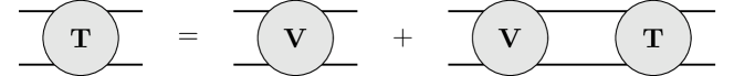
The fully off-shell LS equation for the matrix is illustrated in Fig. 1. The corresponding integral equation in momentum space is given by
| (11) |
where the explicit expression for the two-particle Green function
| (12) |
was used and the regularization of the momentum integration with the cutoff is left implicit. The partial-wave amplitudes are defined as follows:
| (13) |
The phase shift is related to the on-shell partial-wave amplitudes via:
| (14) |
Next, we split the full potential into the long- and short range parts, , and define the scattering amplitude and the Green function for the long-range potential only. This construction is shown diagrammatically in Fig. 2.
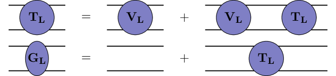
The first line gives the Lippmann-Schwinger for , while the second line gives the expression for in terms of and . Both quantities are needed for the NREFT formulation of the modified effective range expansion. The explicit expressions read
| (15) |
Moreover, we define the short-range matrix ,
| (16) |
which is shown diagrammatically in Fig. 3. Note that the loop integration now involves instead of .

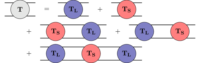
This amounts to adding and dressed by in all possible ways.
The above expressions are of course familiar from the theory of scattering on two potentials. Note that we have used operator notation in Eqs. (2.2, 16, 17) to keep the notation clear. The integrations over intermediate states will only be shown explicitly in the following when required for clarity.
In order to simplify life further, we assume that the long-range potential is repulsive and does not create bound states. Then, the spectral representation of the long-range Green function takes the form:
| (18) |
where denote the eigenfunctions of the Hamiltonian , corresponding to the eigenvalue , and specifies outgoing/ingoing boundary conditions on the wave function. These wave functions can be constructed with the use of the Møller operators:
| (19) |
Now, let us consider Born series for the quantity
| (20) | |||||
where we have used the abbreviation
| (21) |
On the energy shell , the above expression simplifies to
The partial-wave expansion of the asymptotic wave functions is defined as follows:
| (23) |
Furthermore,
| (24) |
where denotes the scattering phase shift in case of the long-range potential only. Now, the partial-wave expansion of the quantity defined in Eq. (2.2) is given by
| (25) |
where
| (26) |
| (27) |
and is equal to the partial-wave amplitude on the energy shell . In analogy to Eq. (14), one may write
| (28) |
Using Eqs. (17) and (25), one finally gets:
| (29) |
2.3 Non-derivative interactions
Let us first restrict ourselves to and assume that only the coupling is different from zero. Then, the potential is separable:
| (30) |
Here, stands for the wave function in the coordinate space. Then, on the energy shell , the S-wave amplitude takes the form
| (31) |
where
| (32) |
Let us now assume that the conditions of Ref. vanHaeringen:1981pb are fulfilled and, namely, the long-range potential is local. It is convenient to define the partial-wave expansion of the Green function in the momentum/coordinate spaces as follows:
| (33) |
with . Then,
| (34) |
Using the result of Appendix A, we can write
| (35) |
where is given by Eq. (4). The real polynomial can be safely dropped as it corresponds to the choice of the renormalization prescription. Next, we require the scattering wave function defined in Eq. (86). Using
| (36) |
along with Eqs. (28) and (31), we obtain
| (37) |
for the S-wave phase shift. The essence of the modified effective-range expansion is now crystal clear: it has a larger radius of convergence which is governed by the short-range potential only.
2.4 Derivative interactions
Consider now the situation when the matrix element of the potential is a generic low-energy polynomial defined in Eq. (10). This is no more true for the potential , defined in Eq. (27). Here, we wish to address the structure of the latter in more detail. The partial-wave expansion of the has the form:
Convoluting Eq. (8) with the wave functions, integrals of the following type emerge
| (38) |
One can now use the identity
| (39) |
and rewrite Eq. (38) as
| (40) |
Here, as in Ref. vanHaeringen:1981pb , it is assumed that the long-range potential is local and spherically symmetric. Furthermore, consider the case first. Using the Schrödinger equation, one then gets
| (41) |
In the case of a regularized Yukawa coupling, the quantity is finite.
Acting now with the operator on both sides of this equation once more, one gets a term, containing , as well as terms with the space derivatives acting on . Continuing this operation, we get a string of terms, containing . Furthermore, owing to the rotational symmetry,
| (44) |
One could stick to the dimensional regularization here, in which all are finite. Furthermore, in the dimensional regularization, , where denotes the small mass scale of the long-distance potential (the pion mass , in case of Yukawa interactions). We remind the reader that we are dealing here with the long-distance (infrared) problems, for which the details of the ultraviolet renormalization should not matter.
The Kronecker -symbols, which are present in Eq. (44), can be further contracted with acting on the wave function, turning them into the Laplacians that can be again eliminated with the use of the Schrödinger equation. At the end of the day, for ,
| (45) |
where the coefficients are expressed through and the derivatives of the potential at the origin. It is important to mention that the mass scale in the derivatives is set by the long-range potential and, therefore, the expansion in the derivatives is converging fast.
Next, consider the case and restore the factor in the expression for . This factor contains exactly derivatives which should be commuted through all potentials to the right. Performing the limit , it is straightforward to ensure that
| (46) | |||||
where
| (47) |
Furthermore, using
| (48) |
one obtains
| (49) |
In the above expression, the couplings are expressed through in form of the series in the small scale . In other words, no unnaturally large couplings emerge. This property is crucial for arguing that the sum, given in the above equation, still represents a low-energy polynomial. To summarize, unlike , is not a low-energy polynomial. The difference is however minimal and boils down to the Jost functions that enter the expression as a multiplicative factor.
At the next step, we carry out the partial-wave expansion in Eq. (26) and use the following ansatz for the partial-wave amplitude:
| (50) |
This gives
Let us now define a new amplitude that obeys an integral equation with a regular kernel:
| (52) | |||||
These two amplitudes on the energy shell are related by
| (53) | |||||
Note that , like , is a low-energy polynomial. Identifying , we obtain:
| (54) |
Finally, using Eqs. (28) and (35), one arrives at the modified effective-range expansion as given in Eq. (3), with being by a low-energy polynomial.
To summarize, using effective field theory methods, we have rederived the modified effective range expansion formula of Ref. vanHaeringen:1981pb , where the effects of the long-range interactions are separated and included in the functions and that do not depend on the short-range potential . This neat separation is, however, based on the assumption that the long-range potential is local. The most important cases of the long-range force: the one-pion exchange as well as Coulomb interactions are exactly of this type. It can be further expected that, with some effort, the method could be generalized to the case of a finite sum , albeit the final formula probably takes a more complicated form (Here, the couplings in front of are assumed to be of natural size.). In this paper, we are not pursuing this idea further. On the other hand, a generic non-local long-range potential (say, a separable potential with a very smooth cutoff) is most likely not amenable to this kind of treatment at all. In other words, in general, there are two mass scales present in the potential – the one associated with the momentum transfer and the one associated with the relative momentum in the CM frame, respectively. A long-range potential, in which the former scale is small whereas the latter scale is of a natural size, can be treated with the method in a similar way as described above.
3 Modified Lüscher equation
3.1 Derivation of the quantization condition
In a finite box, the Green function , which enters in the equation for , can be expanded in a sum over all eigenvectors of the Hamiltonian in a finite volume:
| (55) |
Furthermore, the finite-volume spectrum of the system is determined by the pole positions of the full matrix that can be written down in a form of a finite-volume analog of Eq. (17). Using the fact that the poles of will eventually cancel Doring:2009bi (see also Appendix B), it is straightforward to conclude that the spectrum will be determined by the poles of . Moreover, it is easily seen that no spurious poles emerge, since the poles that emerge in are shifted by the short-range interaction. Using now the basis of eigenfunctions of the Hamiltonian and defining the quantity
| (56) |
we get
| (57) |
(The dependence of on is suppressed hereafter). Furthermore, using the partial-wave expansion
| (58) |
we get
| (59) |
The next steps in the derivation repeat those in the infinite volume. We use following ansatz for the matrix
| (60) |
and get
| (61) | |||||
Define again
| (62) | |||||
The infinite-volume limit in this (subtracted) equation can be performed, and the quantity tends to in this limit. On the mass shell, with we, therefore, obtain
| (63) | |||||
where
| (64) |
The modified quantization condition, derived from Eq. (63) takes the form . Using again, as in Eq. (54), the definition , we arrive at the following expression for the matrix :
| (65) |
3.2 Calculation of the function
Owing to our choice of the superregular long-range potential, the quantity is free of the ultraviolet divergences for . However, one still needs a finite renormalization, in order to ensure that the definition of the function in a finite volume is consistent with its infinite-volume counterpart. Below, we shall consider the cases and separately.
3.2.1 Negative energies,
In the case , a consistent definition of the loop function is given by
| (66) |
It should be mentioned here that the functions and hence are analytic in the upper half of the complex -plane.333Considering the Born series of the Green function , it is easy to get convinced that is real everywhere below threshold. Consequently, is well-defined for negative values of , taking into account the presence of the infinitesimal positive imaginary part in . Furthermore, using Eqs. (2.2), (64) and applying the Poisson formula, one gets:
| (67) |
where
| (68) |
The first term here is the standard Lüscher zeta-function. In order to calculate the remaining two terms, let us consider the Lippmann-Schwinger equation for (a finite-volume counterpart of Eq. (2.2)). Carrying out the partial-wave expansion
| (69) |
one gets
| (70) | |||||
where
| (71) |
The quantity is analytic in the upper half-plane of the variable and vanishes exponentially, when . Note that is always even for identical particles.
For the following discussion, it is convenient to define for negative arguments,
| (72) |
and, hence, from Eq. (70) one concludes that
| (73) | |||||
This means that the integration over the variable can be extended over the whole real axis, from to :
| (74) | |||||
Using now the fact that is analytic in the upper half-plane, one may shift the variables . The value of is restricted by the singularities appearing in the free Green function as well as in the potential . Namely, must fulfill the condition , for the free Green function to stay regular. The restriction coming from the potential does not depend on . For instance, in case of Yukawa interaction, we have . The quantity should obey both conditions. Performing the contour shift in the second and third lines of Eq. (3.2.1) as well, one sees that the finite-volume corrections to are suppressed by the factor .
3.2.2 Positive energies,
For , the Poisson formula can not be used. The infinite-volume limit of the quantity in this case implies using the principal value prescription. Furthermore, from unitarity one can straightforwardly conclude that
| (75) | |||||
where
| (76) |
Here, denotes the -matrix for the scattering on the long-range potential. Furthermore, since, by definition, , with the use of Eqs. (3) and (35) one obtains, on the one hand,
| (77) |
and, on the other hand,
| (78) | |||||
Using now Eq. (2.2) and performing the partial-wave expansion of the on-shell function in analogy with Eq. (85), we obtain:
| (79) |
where is the on-shell wave function. Performing the limit in this equation, we get:
| (80) |
Finally, from Eq. (48), one concludes that Eqs. (77) and (78) are consistent. This represents a nice check of our approach.
A consistent definition of the quantity is given by
| (81) |
where is defined by a counterpart of Eq. (64), with sums replaced by integrals with the principal-value prescription everywhere. Note also that, since the potential is superregular, no ultraviolet divergences arise except in the free loop containing no potential exchange. There, it can be handled, as usual, by using dimensional regularization and cancels anyway in the difference of the finite-volume and the infinite-volume contributions.
Neglecting exponentially suppressed contributions from the long-range interactions, one could reduce the calculation of the function to the solution of the system of linear equations in the angular-momentum basis. This equation has the following form:
| (82) |
Here, are the partial-wave on-shell -matrices, corresponding to the long-range potential, and
| (83) |
This quantity can be expressed through a linear combination of the Lüscher zeta-functions. The quantity should be taken equal to zero in this case.
Note however that neglecting exponential corrections coming from the long-range potential might be dangerous. This is seen, for example, from the fact that, below threshold, , the quantity develops the -channel singularity that was mentioned earlier, whereas the exact function is of course regular there. The derivation of the modified quantization condition, which was presented above, nicely demonstrates the origin of the problem and a way to circumvent it. In fact, the problem is handmade and is not present in Eq. (65). It emerges first, when one tries to evaluate from Eq. (82) and continue analytically below threshold. All this is perfectly consistent with the discussion in the recent paper Raposo:2023oru .
3.3 Partial-wave mixing
Above threshold, the modified zeta-function is determined from Eq. (82) or from the pertinent equation in the plane-wave basis. Since is a long-range potential, it is expected that many partial waves will contribute to this expression. However, this is not a problem, since is a well-known function, with parameters that are determined very precisely elsewhere (e.g., the pion mass and the pion axial-vector coupling, in case of the one-pion exchange potential). Hence, the solution of Eq. (82) does not require a fit to lattice data. On the other hand, the short-range interaction, encoded in the function , is determined from the fit. One expects that the partial-wave mixing effect in the modified Lüscher equation is small, exactly because of the short-range nature of these interactions.
3.4 Exponentially suppressed effects
Up to now, we have consistently dropped the exponentially suppressed effects. However, as mentioned already in the introduction, these effects can turn relatively large, owing to the small mass scale. In the case of, say, scattering, one may indirectly estimate the size of the exponential effects, comparing the finite-volume spectra obtained in the plane-wave basis with the solutions of the modified Lüscher equation with the same input. A simpler method to estimate the size of the exponential effects is the comparison of the modified Lüscher functions , calculated in the plane-wave basis and in the angular-momentum basis. This comparison does not involve any parameters that characterize the short-range interactions.
There is one place, however, where one already knows that the exponential effects are important. We remind the reader that the energy levels, which lie on the -channel cut, are indeed observed in the system on the lattice Green:2021qol . Physical bound states cannot be present there and, hence, the infinite-volume limit of the Lüscher equation does not predict a pole in this region. The observed poles can only emerge because of the exponential contributions.
4 Comparison with the existing approaches
So far, several different frameworks (including the present one) have been proposed to treat the finite-volume scattering in the presence of the long-range forces. All three approaches have one thing in common – namely, they all treat the long-range part of the potential explicitly, without trying to approximate it by a string of contact interactions (like in the derivation of the ordinary Lüscher equation). After that point, the paths start to diverge.
In the recent paper Raposo:2023oru a modified two-body quantization condition has been derived in the presence of both the long- and short-range forces. The authors present their central result in two different forms. Namely, Eq. (3.63) of that paper is written down in a plane wave and angular-momentum basis. From this point of view, it bears strong resemblance with the approach of Ref. Meng:2021uhz , however, with a conceptual difference. Namely, all short-range interactions in Ref. Raposo:2023oru are summed up and enter the quantization condition through an auxiliary on-shell -matrix . No particular parameterization of the on-shell -matrix is specified. We note, however, that for any realistic application to lattice data involving partial-wave mixing such a parameterization would be required. In contrast, the long- and short-range interactions are treated on equal footing in Ref. Meng:2021uhz , and the short-range -matrix is implicitly parameterized in terms of the effective couplings appearing in the Hamiltonian.
Furthermore, in Eqs. (5.3) and (5.4) of Ref. Raposo:2023oru the authors recast their central result in the angular-momentum basis. This result bears close analogy to our modified quantization condition. For example, the quantity from their Eq. (5.4) is similar to our modified Lüscher function . The main difference, as already noted in the introduction, is that the authors of Ref. Raposo:2023oru propose a two-step procedure for the analysis of lattice data. Namely, at the first step, an auxiliary matrix is determined from data. At the next step, is substituted into the integral equation which is solved to obtain the physical -matrix. We propose to unite these two steps in one – in our approach, the auxiliary -matrix is related to the physical one at the same CM energy through a simple algebraic expression.
Last but not least, it has been recently proposed to solve the -channel problem in the two-body scattering by writing down three-body scattering equations Hansen:2024ffk . In particular, the -channel cut that emerges close to threshold in scattering (assuming a stable ) does not show up in the three-body quantization condition for the system, even if the bound state in the subsystem lies below the elastic threshold. The results seems surprising at a first glance. Let us recall however that the three-body quantization condition is written down in the space of spectator momenta. Hence, in case of the stable meson, this approach, up to the exponentially suppressed contributions should be algebraically equivalent to the plane-wave solution proposed in Refs. Meng:2021uhz ; Du:2023hlu ; Meng:2023bmz . Note however that, in difference to the latter, the approach of Ref. Hansen:2024ffk allows for a smooth transition to the case of an unstable meson.444Note also that the calculation of the infinite-volume scattering amplitude in the region of the -channel cut has been carried out earlier in Ref. Dawid:2023jrj . In these calculations it was explicitly shown that the particle-dimer amplitude develops the left-hand singularity. The method of Ref. Hansen:2024ffk essentially stems from this observation.
To summarize, the difference between the existing approaches mainly boils down to the following two points:
-
1.
Technical convenience. The quantization condition can be written down in the plane-wave basis as well as in the angular-momentum basis. Given modern computing capacities, the difference between these two representations is not a decisive factor anymore. Despite this, we still prefer a more compact representation in the angular-momentum basis, which reduces to a single algebraic equation if the partial-wave mixing for the short-range interactions can be neglected. The same statement applies to relating physical observables to quantities extracted from the fit to lattice data. For example, in order to relate to the physical -matrix, integral equations need to be solved Raposo:2023oru , whereas the corresponding link in our approach is given by a simple algebraic relation.
-
2.
The choice of quantities extracted from lattice data. This is a more subtle issue. In an idealized world with single-channel scattering and no partial-wave mixing, the Lüscher equation just gives the scattering phase in terms of the level energy. In realistic situations, however, one often needs a parameterization of the -matrix in order to solve the quantization condition. Without any doubt, the use of an effective Hamiltonian provides such a parameterization within the range of applicability of this particular EFT. In this case, the quantities that are extracted from data at first hand are the couplings of the effective Hamiltonian. However, expressing the lattice energy levels directly in terms of the physical -matrix, in our opinion, renders the approach more flexible: for example, one might use different EFTs (or expansions) in different energy regions to cover a larger energy range.
5 Conclusions
-
i)
In this paper, we have derived a modified Lüscher equation in the presence of both the long-range and short-range interactions. The presence of the former leads to several (interrelated) conceptual difficulties in the standard Lüscher equation. Namely,
-
–
The partial-wave expansion may converge slowly, and hence there could be a significant admixture of the higher partial waves in the Lüscher equation that complicates the analysis of data.
-
–
The long-range interactions lead to a -channel cut in the scattering amplitude that moves very close to the threshold, if the range of the interactions increases. Using lattice energy levels that lie below the -channel threshold in the Lüscher equation is inconsistent.
-
–
The exponentially suppressed contributions could be still significant for not so large values of .
Our approach which, loosely speaking, represents a re-formulation of the modified effective-range expansion of Ref. vanHaeringen:1981pb in a finite volume, is capable to address all above challenges.
-
–
-
ii)
Several alternative approaches have appeared recently in the literature Meng:2021uhz ; Raposo:2023oru ; Hansen:2024ffk . In our paper, a detailed comparison to these approaches is given. We argue that our method is conceptually closest to the original Lüscher framework. It allows to directly extract the scattering phase shift from the measured energy spectrum, if the partial-wave mixing for the short-range interactions is negligible and if the parameters of the long-range potential (i.e., the mass and the coupling of the pion) are known accurately for a given lattice ensemble. Hence, it should be possible to analyze lattice data analog to the original Lüscher approach once the modified Lüscher function is available.
-
iii)
The modified Lüscher function, which incorporates the long-range interaction, is a central ingredient of our approach. In the present paper we consider the evaluation of this function in great detail, paying particular attention to the issues of the ultraviolet divergences and renormalization. Once this function, which does not depend on the unknown parameters of the short-range force, is calculated and tabulated, the analysis of data exactly follows the standard pattern. An explicit calculation of this function is however a rather challenging enterprise and will be discussed in a separate publication.
-
iv)
Note that in this paper we deliberately ignored all issues related with the spin of particles, moving frames, relativistic effects, etc. All this is inessential in the context of the problems considered here and would only blur the discussion.
-
v)
It remains to be seen, whether the Coulomb interaction can be treated consistently in the same manner, and whether the results would add something substantial to the findings of Refs. Beane:2014qha ; Cai:2018why ; Christ:2021guf . Here, it should be also mentioned that, due to the removal of the zero mode of the Coulomb field in case of periodic boundary conditions, the resulting Lagrangian is not local anymore. This, in its turn, might cause problems in the matching of the non-relativistic effective field theory, which is used for the derivation of the Lüscher equation, to its relativistic counterpart (see, e.g., Ref. Davoudi:2018qpl ). In this context, it would be interesting to explore the possibility of using different boundary conditions. An alternative to this would be to use the formulation with massive protons, see, e.g. Endres:2015gda .
-
vi)
The major challenge consists in using the same method in the three-particle problem. For instance, it remains to be seen, whether the long-range one-pion exchange force in the three-nucleon system can be separated as neatly from the short-range interactions as done in case of the nucleon-nucleon scattering.
Acknowledgments: The authors thank Vadim Baru, Evgeny Epelbaum, Jambul Gegelia, Christoph Hanhart, Nils Hermanssohn-Truedsson, Bai-Long Hoid, Lu Meng and Fernando Romero-Lopez for interesting discussions. The work of R.B, F.M. and A.R. was funded in part by the Deutsche Forschungsgemeinschaft (DFG, German Research Foundation) – Project-ID 196253076 – TRR 110 and by the Ministry of Culture and Science of North Rhine-Westphalia through the NRW-FAIR project. A.R., in addition, thanks Volkswagenstiftung (grant no. 93562) and the Chinese Academy of Sciences (CAS) President’s International Fellowship Initiative (PIFI) (grant no. 2024VMB0001) for the partial financial support. The work of J.-Y.P. and J.-J.W. was supported by the National Natural Science Foundation of China (NSFC) under Grants No. 12135011, 12175239, 12221005, and by the National Key R&D Program of China under Contract No. 2020YFA0406400, and by the Chinese Academy of Sciences under Grant No. YSBR-101, and by the Xiaomi Foundation / Xiaomi Young Talents Program. H.-W.H. was supported by Deutsche Forschungsgemeinschaft (DFG, German Research Foundati on) – Project ID 279384907 – SFB 1245.
Appendix A Calculating the Green function
The Green function in the coordinate space can be expressed through the Møller operator
| (84) |
In Ref. Fuda:1973zz , Fuda and Whiting defined the off-shell scattering wave function (cf. with Eq. (2.2)):
| (85) |
This scattering wave function obeys the equation
| (86) |
where
| (87) |
are expressed through the spherical Bessel, Neumann and Hankel functions, respectively. The familiar on-shell wave function is given by .
Using the expansion of the plane wave into spherical functions in Eq. (84), we obtain
| (88) |
Performing the limit , one gets:
| (89) |
where
| (90) |
Note that the same definition of the operator is used, if is replaced by an arbitrary function.
In order to perform the integral over , we rewrite the wave function in terms of the off-shell functions Fuda:1973zz :
| (91) | |||||
where . Here, the function obeys the equation
| (92) |
and has the asymptotic normalization
| (93) |
The off-shell Jost functions are defined as
| (94) |
and the usual Jost functions are obtained from the off-shell Jost functions according to .
Substituting Eq. (91) into Eq. (89), it is seen that the integration can be extended from to , owing to the symmetry of the integrand:
| (95) | |||||
Note that the factor has disappeared, since contains the factor instead of , cf. Eq. (90).
In order to perform the integral by using Cauchy’s theorem, it is important to show that the Jost solutions do not have singularities in the upper complex plane of the variable . To this end, we define the functions
| (96) |
Using Eq. (92) and the asymptotic condition, it can be shown that the function obeys the following integral equation
| (97) | |||||
Solving this equation iteratively, one arrives at
| (98) |
An exact form of the kernel is not important. It suffices to know that the kernel does not depend on and vanishes at . Furthermore, assuming , we get
| (99) |
Acting now with the operator on Eq. (98) and taking the limit , one gets:
| (100) |
Again, , are independent of . Performing now Cauchy integrals, one gets:
| (101) | |||||
Here, one has used the fact that the integral, multiplying , vanishes in the symmetric boundaries. Furthermore
| (102) | |||||
Here, denotes a polynomial of order in the variable . The coefficients of this polynomial are ultraviolet-divergent and can be regularized, e.g., introducing a momentum cutoff on the integration momenta, .
One more remark is in order. It should be pointed out that the final result crucially depends on the validity of Eqs. (101) and (102). Using Cauchy’s theorem straightforwardly is not allowed, since the integrand does not vanish sufficiently fast at the infinity. The result given above corresponds to the choice of symmetric boundary conditions and , which follows from extending the initial integration area by using the fact that the integrand is even under the interchange . The terms containing the potential are vanishing exponentially on a large semicircle in the complex plane, and so Cauchy’s theorem can be used there without further ado.
Appendix B Cancellation of the poles
Using Eq. (17), it is straightforward to see that the full Green function can be espressed as
| (104) |
Our aim is to show that the poles of will cancel in . Note that our reasoning will be valid both in a finite as well as in the infinite volume.
Owing to the spectral representation written down in Eq. (55), in the vicinity of an isolated pole at , the Green function has the following representation:
| (105) |
where is regular at . Furthermore, defining the quantity
| (106) |
which is apparenly regular at , we obtain
| (107) |
It is explicitly seen that this expression does not contain a pole at , if the matrix element in the denominator does not accidentally vanish. Moreover, using Eqs. (105) and (107) in Eq. (104), after a simple algebra one obtains:
| (108) |
Again, the poles that emerge from , have canceled in the final result.
References
- [1] Martin Lüscher. Two particle states on a torus and their relation to the scattering matrix. Nucl. Phys. B, 354:531–578, 1991.
- [2] K. Rummukainen and Steven A. Gottlieb. Resonance scattering phase shifts on a nonrest frame lattice. Nucl. Phys. B, 450:397–436, 1995.
- [3] Michael Lage, Ulf-G. Meißner, and Akaki Rusetsky. A Method to measure the antikaon-nucleon scattering length in lattice QCD. Phys. Lett. B, 681:439–443, 2009.
- [4] V. Bernard, M. Lage, U.-G. Meißner, and A. Rusetsky. Scalar mesons in a finite volume. JHEP, 01:019, 2011.
- [5] Song He, Xu Feng, and Chuan Liu. Two particle states and the S-matrix elements in multi-channel scattering. JHEP, 07:011, 2005.
- [6] Chuan Liu, Xu Feng, and Song He. Two particle states in a box and the S-matrix in multi-channel scattering. Int. J. Mod. Phys. A, 21:847–850, 2006.
- [7] Maxwell T. Hansen and Stephen R. Sharpe. Multiple-channel generalization of Lellouch-Luscher formula. Phys. Rev. D, 86:016007, 2012.
- [8] Raul A. Briceno and Zohreh Davoudi. Moving multichannel systems in a finite volume with application to proton-proton fusion. Phys. Rev. D, 88(9):094507, 2013.
- [9] Ning Li and Chuan Liu. Generalized Lüscher formula in multichannel baryon-meson scattering. Phys. Rev. D, 87(1):014502, 2013.
- [10] Peng Guo, Jozef Dudek, Robert Edwards, and Adam P. Szczepaniak. Coupled-channel scattering on a torus. Phys. Rev. D, 88(1):014501, 2013.
- [11] Luka Leskovec and Sasa Prelovsek. Scattering phase shifts for two particles of different mass and non-zero total momentum in lattice QCD. Phys. Rev. D, 85:114507, 2012.
- [12] C. h. Kim, C. T. Sachrajda, and Stephen R. Sharpe. Finite-volume effects for two-hadron states in moving frames. Nucl. Phys. B, 727:218–243, 2005.
- [13] M. Gockeler, R. Horsley, M. Lage, U.-G. Meißner, P. E. L. Rakow, A. Rusetsky, G. Schierholz, and J. M. Zanotti. Scattering phases for meson and baryon resonances on general moving-frame lattices. Phys. Rev. D, 86:094513, 2012.
- [14] Lu Meng and E. Epelbaum. Two-particle scattering from finite-volume quantization conditions using the plane wave basis. JHEP, 10:051, 2021.
- [15] André Baião Raposo and Maxwell T. Hansen. The Lüscher scattering formalism on the t-channel cut. PoS, LATTICE2022:051, 2023.
- [16] André Baião Raposo and Maxwell T. Hansen. Finite-volume scattering on the left-hand cut. 11 2023.
- [17] Jeremy R. Green, Andrew D. Hanlon, Parikshit M. Junnarkar, and Hartmut Wittig. Weakly bound dibaryon from SU(3)-flavor-symmetric QCD. Phys. Rev. Lett., 127(24):242003, 2021.
- [18] Meng-Lin Du, Arseniy Filin, Vadim Baru, Xiang-Kun Dong, Evgeny Epelbaum, Feng-Kun Guo, Christoph Hanhart, Alexey Nefediev, Juan Nieves, and Qian Wang. Role of Left-Hand Cut Contributions on Pole Extractions from Lattice Data: Case Study for Tcc(3875)+. Phys. Rev. Lett., 131(13):131903, 2023.
- [19] Lu Meng, Vadim Baru, Evgeny Epelbaum, Arseniy A. Filin, and Ashot M. Gasparyan. Solving the left-hand cut problem in lattice QCD: from finite volume energy levels. 12 2023.
- [20] V. Baru, E. Epelbaum, A. A. Filin, and J. Gegelia. Low-energy theorems for nucleon-nucleon scattering at unphysical pion masses. Phys. Rev. C, 92(1):014001, 2015.
- [21] V. Baru, E. Epelbaum, and A. A. Filin. Low-energy theorems for nucleon-nucleon scattering at MeV. Phys. Rev. C, 94(1):014001, 2016.
- [22] Maxwell T. Hansen and Stephen R. Sharpe. Relativistic, model-independent, three-particle quantization condition. Phys. Rev., D90(11):116003, 2014.
- [23] Maxwell T. Hansen and Stephen R. Sharpe. Expressing the three-particle finite-volume spectrum in terms of the three-to-three scattering amplitude. Phys. Rev., D92(11):114509, 2015.
- [24] Hans-Werner Hammer, Jin-Yi Pang, and A. Rusetsky. Three-particle quantization condition in a finite volume: 1. The role of the three-particle force. JHEP, 09:109, 2017.
- [25] H. W. Hammer, J. Y. Pang, and A. Rusetsky. Three particle quantization condition in a finite volume: 2. General formalism and the analysis of data. JHEP, 10:115, 2017.
- [26] M. Mai and M. Döring. Three-body Unitarity in the Finite Volume. Eur. Phys. J., A53(12):240, 2017.
- [27] Maxim Mai and Michael Döring. Finite-Volume Spectrum of and Systems. Phys. Rev. Lett., 122(6):062503, 2019.
- [28] Maxwell T. Hansen, Fernando Romero-López, and Stephen R. Sharpe. Incorporating effects and left-hand cuts in lattice QCD studies of the . 1 2024.
- [29] Silas R. Beane and Martin J. Savage. Two-Particle Elastic Scattering in a Finite Volume Including QED. Phys. Rev. D, 90(7):074511, 2014.
- [30] Yiming Cai and Zohreh Davoudi. QED-corrected Lellouch-Luescher formula for decay. PoS, LATTICE2018:280, 2018.
- [31] Norman Christ, Xu Feng, Joseph Karpie, and Tuan Nguyen. - scattering, QED, and finite-volume quantization. Phys. Rev. D, 106(1):014508, 2022.
- [32] H. van Haeringen and L. P. Kok. Modified Effective Range Function. Phys. Rev. A, 26:1218–1225, 1982.
- [33] Xinwei Kong and Finn Ravndal. Coulomb effects in low-energy proton proton scattering. Nucl. Phys. A, 665:137–163, 2000.
- [34] A. M. Badalian, L. P. Kok, M. I. Polikarpov, and Yu. A. Simonov. Resonances in Coupled Channels in Nuclear and Particle Physics. Phys. Rept., 82:31–177, 1982.
- [35] Marvin L. Goldberger and Kenneth M. Watson. Collision Theory. Dover Publications, 10 2004.
- [36] Michael C. Birse, Judith A. McGovern, and Keith G. Richardson. A Renormalization group treatment of two-body scattering. Phys. Lett. B, 464:169–176, 1999.
- [37] James V. Steele and R. J. Furnstahl. Removing pions from two nucleon effective field theory. Nucl. Phys. A, 645:439–461, 1999.
- [38] M. Doring, C. Hanhart, F. Huang, S. Krewald, and U. G. Meissner. The Role of the background in the extraction of resonance contributions from meson-baryon scattering. Phys. Lett. B, 681:26–31, 2009.
- [39] Sebastian M. Dawid, Md Habib E. Islam, and Raúl A. Briceño. Analytic continuation of the relativistic three-particle scattering amplitudes. Phys. Rev. D, 108(3):034016, 2023.
- [40] Zohreh Davoudi, James Harrison, Andreas Jüttner, Antonin Portelli, and Martin J. Savage. Theoretical aspects of quantum electrodynamics in a finite volume with periodic boundary conditions. Phys. Rev. D, 99(3):034510, 2019.
- [41] Michael G. Endres, Andrea Shindler, Brian C. Tiburzi, and Andre Walker-Loud. Massive photons: an infrared regularization scheme for lattice QCD+QED. Phys. Rev. Lett., 117(7):072002, 2016.
- [42] Michael G. Fuda and James S. Whiting. Generalization of the Jost Function and Its Application to Off-Shell Scattering. Phys. Rev. C, 8:1255–1261, 1973.