Efficient adjustment for complex covariates:
Gaining efficiency with DOPE

Abstract.

Covariate adjustment is a ubiquitous method used to estimate the average treatment effect (ATE) from observational data. Assuming a known graphical structure of the data generating model, recent results give graphical criteria for optimal adjustment, which enables efficient estimation of the ATE. However, graphical approaches are challenging for high-dimensional and complex data, and it is not straightforward to specify a meaningful graphical model of non-Euclidean data such as texts. We propose an general framework that accommodates adjustment for any subset of information expressed by the covariates. We generalize prior works and leverage these results to identify the optimal covariate information for efficient adjustment. This information is minimally sufficient for prediction of the outcome conditionally on treatment.

Based on our theoretical results, we propose the Debiased Outcome-adapted Propensity Estimator (DOPE) for efficient estimation of the ATE, and we provide asymptotic results for the DOPE under general conditions. Compared to the augmented inverse propensity weighted (AIPW) estimator, the DOPE can retain its efficiency even when the covariates are highly predictive of treatment. We illustrate this with a single-index model, and with an implementation of the DOPE based on neural networks, we demonstrate its performance on simulated and real data. Our results show that the DOPE provides an efficient and robust methodology for ATE estimation in various observational settings.

1. Introduction

Estimating the population average treatment effect (ATE) of a treatment on an outcome variable is a fundamental statistical task. A naive approach is to contrast the mean outcome of a treated population with the mean outcome of an untreated population. Using observational data this is, however, generally a flawed approach due to confounding. If the underlying confounding mechanisms are captured by a set of pre-treatment covariates $\mathbf{W}$, it is possible to adjust for confounding by conditioning on $\mathbf{W}$ in a certain manner. Given that multiple subsets of $\mathbf{W}$ may be valid for this adjustment, it is natural to ask if there is an ‘optimal adjustment subset’ that enables the most efficient estimation of the ATE.

Assuming a causal linear graphical model, Henckel et al. (2022) established the existence of – and gave graphical criteria for – an optimal adjustment set for the OLS estimator. Rotnitzky & Smucler (2020) extended the results of Henckel et al. (2022), by proving that the optimality was valid within general causal graphical models and for all regular and asymptotically linear estimators. Critically, this line of research assumes knowledge of the underlying graphical structure.

To accommodate the assumption of no unmeasured confounding, observational data is often collected with as many covariates as possible, which means that $\mathbf{W}$ can be high-dimensional. In such cases, assumptions of a known graph are unrealistic, and graphical estimation methods are statistically unreliable (Uhler et al., 2013; Shah & Peters, 2020; Chickering et al., 2004). Furthermore, for non-Euclidean data such as images or texts, it is not clear how to impose any graphical structure pertaining to causal relations. Nevertheless, we can in these cases still imagine that the information that $\mathbf{W}$ represents can be separated into distinct components that affect treatment and outcome directly, as illustrated in Figure 1.

Figure 1. The covariate $\mathbf{W}$ can have a complex data structure, even if the information it represents is structured and can be categorized into components that influence treatment and outcome separately.

In this paper, we formalize this idea and formulate a novel and general adjustment theory with a focus on efficiency bounds for the estimation of the average treatment effect. Based on the adjustment theory, we propose a general estimation procedure and analyze its asymptotic behavior.

1.1. Setup

Throughout we consider a discrete treatment variable $T\in\mathbb{T}$, a square-integrable outcome variable $Y\in$, and pre-treatment covariates $\mathbf{W}\in\mathbb{W}$. For now we only require that $\mathbb{T}$ is a finite set and that $\mathbb{W}$ is a measurable space. The joint distribution of $(T,\mathbf{W},Y)$ is denoted by $P$ and it is assumed to belong to a collection of probability measures $\mathcal{P}$. If we need to make the joint distribution explicit, we denote expectations and probabilities with $\mathbb{E}_{P}$ and $\mathbb{P}_{P}$, respectively, but usually the $P$ is omitted for ease of notation.

Our model-free target parameters of interest are of the form

(1) $$\chi_{t}\coloneq\mathbb{E}[\mathbb{E}[Y\,|\,T=t,\mathbf{W}]]=\mathbb{E}\left[\frac{\mathbbl{1}(T=t)Y}{\mathbb{P}(T=t\,|\,\mathbf{W})}\right],\qquad t\in\mathbb{T}.$$

In words, these are treatment specific means of the outcome when adjusting for the covariate $\mathbf{W}$. To ensure that this quantity is well-defined, we assume the following condition, commonly known as positivity.

Assumption 1.1 (Positivity).

It holds that $0<\mathbb{P}(T=t\,|\,\mathbf{W})<1$ almost surely for each $t\in\mathbb{T}$.

Under additional assumptions common in causal inference literature – which informally entail that $\mathbf{W}$ captures all confounding – the target parameter $\chi_{t}$ has the interpretation as the interventional mean, which is expressed by $\mathbb{E}[Y\,|\,\mathrm{do}(T=t)]$ in do-notation or by $\mathbb{E}[Y^{t}]$ using potential outcome notation (Peters et al., 2017; van der Laan & Rose, 2011). Under such causal assumptions, the average treatment effect is identified, and when $\mathbb{T}=\{0,1\}$ it is typically expressed as the contrast $\chi_{1}-\chi_{0}$. The theory in this paper is agnostic with regards to whether or not $\chi_{t}$ has this causal interpretation, although it is the primary motivation for considering $\chi_{t}$ as a target parameter.

Given $n$ i.i.d. observations of $(T,\mathbf{W},Y)$, one may proceed to estimate $\chi_{t}$ by estimating either of the equivalent expressions for $\chi_{t}$ in Equation (1). Within parametric models, the outcome regression function

$$g(t,\mathbf{w})=\mathbb{E}[Y\,|\,T=t,\mathbf{W}=\mathbf{w}]$$

can typically be estimated with a $\sqrt{n}$-rate. In this case, the sample mean of the estimated regression function yields a $\sqrt{n}$-consistent estimator of $\chi_{t}$ under Donsker class conditions or sample splitting. However, many contemporary datasets indicate that parametric model-based regression methods get outperformed by nonparametric methods such as boosting and neural networks (Bojer & Meldgaard, 2021).

Nonparametric estimators of the regression function typically converge at rates slower than $\sqrt{n}$, and likewise for estimators of the propensity score

$$m(t\mid\mathbf{w})=\mathbb{P}(T=t\,|\,\mathbf{W}=\mathbf{w}).$$

Even if both nonparametric estimators have rates slower than $\sqrt{n}$, it is in some cases possible to achieve a $\sqrt{n}$-rate of $\chi_{t}$ by modeling both $m$ and $g$, and then combining their estimates in a way that achieves ‘rate double robustness’ (Smucler et al., 2019). That is, an estimation error of the same order as the product of the errors for $m$ and $g$. Two prominent estimators that have this property are the Augmented Inverse Probability Weighted estimator (AIPW) and the Targeted Minimum Loss-based Estimator (TMLE) (Robins & Rotnitzky, 1995; Chernozhukov et al., 2018; van der Laan & Rose, 2011).

In what follows, the premise is that even with a $\sqrt{n}$-rate estimator of $\chi_{t}$, it might still be intractable to model $m$ – and possibly also $g$ – as a function of $\mathbf{W}$ directly. This can happen for primarily two reasons: (i) the sample space $\mathbb{W}$ is high-dimensional or has a complex structure, or (ii) the covariate is highly predictive of treatment, leading to unstable predictions of the inverse propensity score $\mathbb{P}(T=t\,|\,\mathbf{W})^{-1}$.

In either of these cases, which are not exclusive, we can try to manage these difficulties by instead working with a representation $\mathbf{Z}=\varphi(\mathbf{W})$, given by a measurable mapping $\varphi$ from $\mathbb{W}$ into a more tractable space such as ^d. In the first case above, such a representation might be a pre-trained word embedding, e.g., the celebrated BERT and its offsprings (Devlin et al., 2018). The second case has been well-studied in the special case where $\mathbb{W}=^{k}$ and where $\mathcal{P}$ contains the distributions that are consistent with respect to a fixed DAG (or CPDAG). We develop a general theory that subsumes both cases, and we discuss how to represent the original covariates to efficiently estimate the adjusted mean $\chi_{t}$.

1.2. Relations to existing literature

Various studies have explored the adjustment for complex data structures by utilizing a (deep) representation of the covariates, as demonstrated in works such as Shi et al. (2019); Veitch et al. (2020). In a different research direction, the Collaborative TMLE (van der Laan & Gruber, 2010) has emerged as a robust method for estimating average treatment effects by collaboratively learning the outcome regression and propensity score, particularly in scenarios where covariates are highly predictive of treatment (Ju et al., 2019). Our overall estimation approach shares similarities with the mentioned strategies; for instance, our proof-of-concept estimator in the experimental section employs neural networks with shared layers. However, unlike the cited works, it incorporates the concept of efficiently tuning the representation specifically for predicting outcomes, rather than treatment. Related to this idea is another interesting line of research, which builds upon the outcome adapted lasso proposed by Shortreed & Ertefaie (2017). Such works include Ju et al. (2020); Benkeser et al. (2020); Greenewald et al. (2021); Baldé et al. (2023). These works all share the common theme of proposing estimation procedures that select covariates based on $L_{1}$-penalized regression onto the outcome, and then subsequently estimate the propensity score based on the selected covariates adapted to the outcome. The theory of this paper generalizes the particular estimators proposed in the previous works, and also allows for other feature selection methods than $L_{1}$-penalization. Moreover, our generalization of (parts of) the efficient adjustment theory from Rotnitzky & Smucler (2020) allows us to theoretically quantify the efficiency gains from these estimation methods. Finally, our asymptotic theory considers a novel regime, which, according to the simulations, seems more adequate for describing the finite sample behavior than the asymptotic results of Benkeser et al. (2020) and Ju et al. (2020).

Our general adjustment results in Section 3 draws on the vast literature on classical adjustment and confounder selection, for example Rosenbaum & Rubin (1983); Hahn (1998); Henckel et al. (2022); Rotnitzky & Smucler (2020); Guo et al. (2022); Perković et al. (2018); Peters et al. (2017); Forré & Mooij (2023). In particular, two of our results are direct extensions of results from Rotnitzky & Smucler (2020); Henckel et al. (2022).

1.3. Organization of the paper

In Section 2 we discuss generalizations of classical adjustment concepts to abstract conditioning on information. In Section 3 we discuss information bounds in the framework of Section 2. In Section 4 we propose a novel method, the DOPE, for efficient estimation of adjusted means, and we discuss the asymptotic behavior of the resulting estimator. In Section 5 we implement the DOPE and demonstrate its performance on synthetic and real data. The paper is concluded by a discussion in Section 6.

2. Generalized adjustment concepts

In this section we discuss generalizations of classical adjustment concepts. These generalizations are motivated by the premise from the introduction: it might be intractable to model the propensity score directly as a function of $\mathbf{W}$, so instead we consider adjusting for a representation $\mathbf{Z}=\varphi(\mathbf{W})$. This is, in theory, confined to statements about conditioning on $\mathbf{Z}$, and is therefore equivalent to adjusting for any representation of the form $\widetilde{\mathbf{Z}}=\psi\circ\varphi(\mathbf{W})$, where $\psi$ is a bijective and bimeasureable mapping. The equivalence class of such representations is characterized by the $\sigma$-algebra generated by $\mathbf{Z}$, denoted by $\sigma(\mathbf{Z})$, which informally describes the information contained in $\mathbf{Z}$. In view of this, we define adjustment with respect to sub $\sigma$-algebras contained in $\sigma(\mathbf{W})$.

Remark 2.1.

Conditional expectations and probabilities are, unless otherwise indicated, defined conditionally on $\sigma$-algebras as in Kolmogoroff (1933), see also Kallenberg (2021, Ch. 8). Equalities between conditional expectations are understood to hold almost surely. When conditioning on the random variable $T$ and a $\sigma$-algebra $\mathcal{Z}$ we write ‘$\,|\,T,\mathcal{Z}$’ as a shorthand for ‘$\,|\,\sigma(T)\vee\mathcal{Z}$’. Finally, we define conditioning on both the event $(T=t)$ and on a $\sigma$-algebra $\mathcal{Z}\subseteq\sigma(\mathbf{W})$ by $\mathbb{E}[Y\,|\,T=t,\mathcal{Z}]\coloneq\frac{\mathbb{E}[Y\mathbbl{1}(T=t)\,|\,\mathcal{Z}]}{\mathbb{P}(T=t\,|\,\mathcal{Z})},$ which is well-defined under Assumption 1.1. ∎

Definition 2.2.

A sub $\sigma$-algebra $\mathcal{Z}\subseteq\sigma(\mathbf{W})$ is called a description of $\mathbf{W}$. For each $t\in\mathbb{T}$ and $P\in\mathcal{P}$, and with $\mathcal{Z}$ a description of $\mathbf{W}$, we define

$$\pi_{t}(\mathcal{Z};P) \coloneq\mathbb{P}_{P}(T=t\,|\,\mathcal{Z}),$$

$$b_{t}(\mathcal{Z};P) \coloneq\mathbb{E}_{P}[Y\,|\,T=t,\mathcal{Z}],$$

$$\chi_{t}(\mathcal{Z};P) \coloneq\mathbb{E}_{P}[b_{t}(\mathcal{Z};P)]=\mathbb{E}_{P}[\pi_{t}(\mathcal{Z};P)^{-1}\mathbbl{1}(T=t)Y].$$

If a description $\mathcal{Z}$ of $\mathbf{W}$ is given as $\mathcal{Z}=\sigma(\mathbf{Z})$ for a representation $\mathbf{Z}=\varphi(\mathbf{W})$, we may write $\chi_{t}(\mathbf{Z};P)$ instead of $\chi_{t}(\sigma(\mathbf{Z});P)$ etc.

We say that

$$\mathcal{Z} P \qquad\chi_{t}(\mathcal{Z};P)=\chi_{t}(\mathbf{W};P), \text{ for all }t\in\mathbb{T},$$ is -valid if:

$$\mathcal{Z} P \qquad b_{t}(\mathcal{Z};P)=b_{t}(\mathbf{W};P), \text{ for all }t\in\mathbb{T},$$ is -OMS if:

$$\mathcal{Z} P \qquad Y\,{\perp\!\!\!\perp}_{P}\,\mathbf{W}\,|\,T,\mathcal{Z}.$$ is -ODS if:

Here OMS means Outcome Mean Sufficient and ODS means Outcome Distribution Sufficient. If $\mathcal{Z}$ is $P$-valid for all $P\in\mathcal{P}$, we say that it is $\mathcal{P}$-valid. We define $\mathcal{P}$-OMS and $\mathcal{P}$-ODS analogously. ∎

A few remarks are in order.

• We have implicitly extended the shorthand notation described in Remark 2.1 to the quantities in Definition 2.2.

• The quantity $\chi_{t}(\mathcal{Z};P)$ is deterministic, whereas $\pi_{t}(\mathcal{Z};P)$ and $b_{t}(\mathcal{Z};P)$ are $\mathcal{Z}$-measurable real valued random variables. Thus, if $\mathcal{Z}$ is generated by a representation $\mathbf{Z}$, then by the Doob-Dynkin lemma (Kallenberg, 2021, Lemma 1.14) these random variables can be expressed as functions of $\mathbf{Z}$. This fact does not play a role until the discussion of estimation in Section 4.

• There are examples of descriptions $\mathcal{Z}\subseteq\sigma(\mathbf{W})$ that are not given by representations. Such descriptions might be of little practical importance, but our results do not require $\mathcal{Z}$ to be given by a representation. We view the $\sigma$-algebraic framework as a convenient abstraction that generalizes equivalence classes of representations.

• We have the following hierarchy of the properties in Definition 2.2:

  $$P\textnormal{-ODS}\Longrightarrow P\textnormal{-OMS}\Longrightarrow P\textnormal{-valid},$$

  and the relations also hold if $P$ is replaced by $\mathcal{P}$.

• The $P$-ODS condition relates to existing concepts in statistics. The condition can be viewed as a $\sigma$-algebraic analogue of prognostic scores (Hansen, 2008), and it holds that any prognostic score generates a $P$-ODS description. Moreover, if a description $\mathcal{Z}=\sigma(\mathbf{Z})$ is $P$-ODS, then its generator $\mathbf{Z}$ is $c$-equivalent to $\mathbf{W}$ in the sense of Pearl (2009), see in particular the claim following his Equation (11.8). In Remark 3.12 we discuss the relations between $\mathcal{P}$-ODS descriptions and classical statistical sufficiency.

The notion of $\mathcal{P}$-valid descriptions can be viewed as a generalization of valid adjustment sets, where subsets are replaced with sub $\sigma$-algebras.

Example 2.3 (Comparison with adjustment sets in causal DAGs).

Suppose $\mathbf{W}\in^{k}$ and let $\mathcal{D}$ be a DAG on the nodes $\mathbf{V}=(T,\mathbf{W},Y)$. Let $\mathcal{P}=\mathcal{M}(\mathcal{D})$ be the collection of continuous distributions (on ^k+2) that are Markovian with respect to $\mathcal{D}$ and with $\mathbb{E}|Y|<\infty$.

Any subset $\mathbf{Z}\subseteq\mathbf{W}$ is a representation of $\mathbf{W}$ given by a coordinate projection, and the corresponding $\sigma$-algebra $\sigma(\mathbf{Z})$ is a description of $\mathbf{W}$. In this framework, a subset $\mathbf{Z}\subseteq\mathbf{W}$ is called a valid adjustment set for $(T,Y)$ if for all $P\in\mathcal{P}$, $t\in\mathbb{T}$, and $y\in$

$$\mathbb{E}_{P}\left[\frac{\mathbbl{1}(T=t)\mathbbl{1}(Y\leq y)}{\mathbb{P}_{P}(T=t\,|\,\mathrm{pa}_{\mathcal{D}}(T))}\right]=\mathbb{E}_{P}[\mathbb{P}_{P}(Y\leq y\,|\,T=t,\mathbf{Z})],$$

see, e.g., Definition 2 in Rotnitzky & Smucler (2020). It turns out that $\mathbf{Z}$ is a valid adjustment set if and only if

$$\mathbb{E}_{P}\left[\frac{\mathbbl{1}(T=t)Y}{\mathbb{P}_{P}(T=t\,|\,\mathrm{pa}_{\mathcal{D}}(T))}\right]=\mathbb{E}_{P}[\mathbb{E}_{P}[Y\,|\,T=t,\mathbf{Z}]]=\chi_{t}(\mathcal{Z};P)$$

for all $P\in\mathcal{P}$ and $t\in\mathbb{T}$. This follows from results of Perković et al. (2018), which we discuss for completeness in Proposition A.1. Thus, if we assume that $\mathbf{W}$ is a valid adjustment set, then any subset $\mathbf{Z}\subseteq\mathbf{W}$ is a valid adjustment set if and only if the corresponding description $\sigma(\mathbf{Z})$ is $\mathcal{P}$-valid. ∎

In general, $\mathcal{P}$-valid descriptions are not necessarily generated from valid adjustment sets. This can happen if structural assumptions are imposed on the conditional mean, which is illustrated in the following example.

Example 2.4.

Suppose that the outcome regression is known to be invariant under rotations of $\mathbf{W}\in^{k}$ such that for any $P\in\mathcal{P}$,

$$\mathbb{E}_{P}[Y\,|\,T,\mathbf{W}]=\mathbb{E}_{P}[Y\,|\,T,\|\mathbf{W}\|\,]\eqcolon g_{P}(T,\|\mathbf{W}\|).$$

Without further graphical assumptions, we cannot deduce that any proper subset of $\mathbf{W}$ is a valid adjustment set. In contrast, the magnitude $\|\mathbf{W}\|$ generates a $\mathcal{P}$-OMS – and hence also $\mathcal{P}$-valid – description of $\mathbf{W}$ by definition.

Suppose that there is a distribution $\tilde{P}\in\mathcal{P}$ for which $g_{\tilde{P}}(t,\cdot)$ is bijective. Then $\sigma(\|\mathbf{W}\|)$ is also the smallest $\mathcal{P}$-OMS description up to $\mathbb{P}_{\tilde{P}}$-negligible sets: if $\mathcal{Z}$ is another $\mathcal{P}$-OMS description, we see that $b_{t}(\mathcal{Z};\tilde{P})=b_{t}(\mathbf{W};\tilde{P})=g_{\tilde{P}}(t,\|\mathbf{W}\|)$ almost surely. Hence

$$\sigma(\|\mathbf{W}\|)=\sigma(g_{\tilde{P}}(t,\|\mathbf{W}\|))\subseteq\overline{\sigma(b_{t}(\mathcal{Z};\tilde{P}))}\subseteq\overline{\mathcal{Z}},$$

where overline denotes the $\mathbb{P}_{\tilde{P}}$-completion of a $\sigma$-algebra. That is, $\overline{\mathcal{Z}}$ is the smallest $\sigma$-algebra containing $\mathcal{Z}$ and all its $\mathbb{P}_{\tilde{P}}$-negligible sets. ∎

Even in the above example, where the regression function is known to depend on a one-dimensional function of $\mathbf{W}$, it is generally not possible to estimate the regression function at a $\sqrt{n}$-rate without restrictive assumptions. Thus, modeling of the propensity score is required in order to obtain a $\sqrt{n}$-rate estimator of the adjusted mean. If $\mathbf{W}$ is highly predictive of treatment, then naively applying a doubly robust estimator (AIPW, TMLE) can be statistically unstable due to large inverse propensity weights. Alternatively, since $\sigma(\|\mathbf{W}\|)$ is a $\mathcal{P}$-valid description, we could also base our estimator on the pruned propensity $\mathbb{P}(T=t\,|\,\|\mathbf{W}\|)$. This approach should intuitively provide more stable weights, as we expect $\|\mathbf{W}\|$ to be less predictive of treatment. We proceed to analyze the difference between the asymptotic efficiencies of the two approaches and we show that, under reasonable conditions, the latter approach is never worse asymptotically.

3. Efficiency bounds for adjusted means

We now discuss efficiency bounds based on the concepts introduced in Section 2. To this end, let $\mathbf{Z}=\varphi(\mathbf{W})$ be a representation of $\mathbf{W}$. Under a sufficiently dense model $\mathcal{P}$, the influence function for $\chi_{t}(\mathbf{Z};P)$ is given by

(2) $$\psi_{t}(\mathbf{Z};P)=b_{t}(\mathbf{Z};P)+\frac{\mathbbl{1}(T=t)}{\pi_{t}(\mathbf{Z};P)}(Y-b_{t}(\mathbf{Z};P))-\chi_{t}(\mathbf{Z};P).$$

The condition that $\mathcal{P}$ is sufficiently dense entails that no ‘structural assumptions’ are imposed on the functional forms of $\pi_{t}$ and $b_{t}$, see also Robins et al. (1994); Robins & Rotnitzky (1995); Hahn (1998). Structural assumptions do not include smoothness conditions, but do include, for example, parametric model assumptions on the outcome regression.

Using the formalism of Section 2, we define $\psi_{t}(\mathcal{Z};P)$ analogously to (2) for any description $\mathcal{Z}$ of $\mathbf{W}$. We denote the variance of the influence function by

$$\mathbb{V}_{t}(\mathcal{Z};P) \coloneq\operatorname{Var}_{P}[\psi_{t}(\mathcal{Z};P)]$$

(3) $$=\mathbb{E}_{P}\left[\frac{\operatorname{Var}_{P}(Y\,|\,T=t,\mathcal{Z})}{\pi_{t}(\mathcal{Z};P)}\right]+\operatorname{Var}_{P}(b_{t}(\mathcal{Z};P)).$$

The importance of this variance was highlighted by Hahn (1998), who computed $\mathbb{V}_{t}(\mathbf{W};P)$ as the semiparametric efficiency bound for regular asymptotically linear (RAL) estimators of $\chi_{t}(\mathbf{W};P)$. That is, for any $\mathcal{P}$-consistent RAL estimator $\widehat{\chi}_{t}(\mathbf{W};P)$ based on $n$ i.i.d. observations, the asymptotic variance of $\sqrt{n}(\widehat{\chi}_{t}(\mathbf{W};P)-\chi_{t}(\mathbf{W};P))$ is bounded below by $\mathbb{V}_{t}(\mathbf{W};P)$, provided that $\mathcal{P}$ does not impose structural assumptions on $\pi_{t}(\mathbf{W})$ and $b_{t}(\mathbf{W})$. Moreover, the asymptotic variance of both the TMLE and AIPW estimators achieve this lower bound when the propensity score and outcome regression can be estimated with sufficiently fast rates (Chernozhukov et al., 2018; van der Laan & Rose, 2011).

Since the same result can be applied for the representation $\mathbf{Z}=\varphi(\mathbf{W})$, we see that estimation of $\chi_{t}(\mathbf{Z};P)$ has a semiparametric efficiency bound of $\mathbb{V}_{t}(\mathbf{Z};P)$. Now suppose that $\sigma(\mathbf{Z})$ is a $\mathcal{P}$-valid description of $\mathbf{W}$, which means that $\chi_{t}\coloneq\chi_{t}(\mathbf{W};P)=\chi_{t}(\mathbf{Z};P)$ for all $P$. It is then natural to ask if we should estimate $\chi_{t}$ based on $\mathbf{W}$ or the representation $\mathbf{Z}$? We proceed to investigate this question based on which of the efficiency bounds $\mathbb{V}_{t}(\mathbf{Z};P)$ or $\mathbb{V}_{t}(\mathbf{W};P)$ is smallest.

If $\mathbb{V}_{t}(\mathbf{Z};P)$ is smaller than $\mathbb{V}_{t}(\mathbf{W};P)$, then $\mathbb{V}_{t}(\mathbf{W};P)$ is not an actual efficiency bound for $\chi_{t}(\mathbf{W};P)$. This does not contradict the result of Hahn (1998), as we have assumed the existence of a non-trivial $\mathcal{P}$-valid description of $\mathbf{W}$, which implicitly imposes structural assumptions on the functional form of $b_{t}(\mathbf{W})$. Nevertheless, it is sensible to compare the variances $\mathbb{V}_{t}(\mathbf{Z};P)$ and $\mathbb{V}_{t}(\mathbf{W};P)$, as these are the asymptotic variances of the AIPW when using either $\mathbf{Z}$ or $\mathbf{W}$, respectively, as a basis for the nuisance functions.

We formulate our efficiency bounds in terms of the more general contrast parameter

(4) $$\Delta=\Delta(\mathbf{W};P)=\sum_{t\in\mathbb{T}}c_{t}\chi_{t}(\mathbf{W};P),$$

where $\mathbf{c}\coloneq(c_{t})_{t\in\mathbb{T}}$ are fixed real-valued coefficients. The prototypical example, when $\mathbb{T}=\{0,1\}$, is $\Delta=\chi_{1}-\chi_{0}$, which is the average treatment effect under causal assumptions, cf. the discussion following Assumption 1.1. Note that the family of $\Delta$-parameters includes the adjusted mean $\chi_{t}$ as a special case.

To estimate $\Delta$, we consider estimators of the form

(5) $$\widehat{\Delta}(\mathcal{Z};P)=\sum_{t\in\mathbb{T}}c_{t}\widehat{\chi}_{t}(\mathcal{Z};P),$$

where $\widehat{\chi}_{t}(\mathcal{Z};P)$ denotes a consistent RAL estimator of $\chi_{t}(\mathcal{Z};P)$. Correspondingly, the efficiency bound for such an estimator is

(6) $$\mathbb{V}_{\!\Delta}(\mathcal{Z};P)\coloneq\operatorname{Var}_{P}\Big{(}\sum_{t\in\mathbb{T}}c_{t}\psi_{t}(\mathcal{Z};P)\Big{)}.$$

It turns out that two central results by Rotnitzky & Smucler (2020), specifically their Lemmas 4 and 5, can be generalized from covariate subsets to descriptions. One conceptual difference is that there is a priori no natural generalization of precision variables and overadjustment (instrumental) variables. To wit, if $\mathcal{Z}_{1}$ and $\mathcal{Z}_{2}$ are descriptions, there is no canonical way to subtract $\mathcal{Z}_{2}$ from $\mathcal{Z}_{1}$ in a way that maintains their join $\mathcal{Z}_{1}\vee\mathcal{Z}_{2}\coloneq\sigma(\mathcal{Z}_{1},\mathcal{Z}_{2})$. Apart from this technical detail, the proofs translate more or less directly. The following lemma is a direct extension of Rotnitzky & Smucler (2020, Lemma 4).

Lemma 3.1 (Deletion of overadjustment).

Fix a distribution $P\in\mathcal{P}$ and let $\mathcal{Z}_{1}\subseteq\mathcal{Z}_{2}$ be $\sigma$-algebras such that $Y\,{\perp\!\!\!\perp}_{P}\,\mathcal{Z}_{2}\,|\,T,\mathcal{Z}_{1}$. Then it always holds that

$$\mathbb{V}_{\!\Delta}(\mathcal{Z}_{2};P)-\mathbb{V}_{\!\Delta}(\mathcal{Z}_{1};P)=\sum_{t\in\mathbb{T}}c_{t}^{2}D_{t}(\mathcal{Z}_{1},\mathcal{Z}_{2};P)\geq 0,$$

where for each $t\in\mathbb{T}$,

$$D_{t} (\mathcal{Z}_{1},\mathcal{Z}_{2};P)\coloneq\mathbb{V}_{t}(\mathcal{Z}_{2};P)-\mathbb{V}_{t}(\mathcal{Z}_{1};P)$$

$$=\mathbb{E}_{P}\,\Big{[}\pi_{t}(\mathcal{Z}_{1};P)\operatorname{Var}(Y\,|\,T=t,\mathcal{Z}_{1})\operatorname{Var}\big{(}\pi_{t}(\mathcal{Z}_{2};P)^{-1}\big{|}\;T=t,\mathcal{Z}_{1}\big{)}\Big{]}.$$

Moreover, if $\mathcal{Z}_{2}$ is a description of $\mathbf{W}$ then $\mathcal{Z}_{1}$ is $P$-valid if and only if $\mathcal{Z}_{2}$ is $P$-valid.

The lemma quantifies the efficiency lost in adjustment when adding information that is irrelevant for the outcome.

We proceed to apply this lemma to the minimal information in $\mathbf{W}$ that is predictive of $Y$ conditionally on $T$. To define this information, we use the regular conditional distribution function of $Y$ given $T=t,\mathbf{W}=\mathbf{w}$, which we denote by

$$F(y\,|\,t,\mathbf{w};P)\coloneq\mathbb{P}_{P}(Y\leq y\,|\,T=t,\mathbf{W}=\mathbf{w}),\qquad y\in,t\in\mathbb{T},\mathbf{w}\in\mathbb{W}.$$

See Kallenberg (2021, Sec. 8) for a rigorous treatment of regular conditional distributions. We will in the following, by convention, take

(7) $$b_{t}(\mathbf{w};P)=\int y\,\mathrm{d}F(y\,|\,t,\mathbf{w};P),$$

so that $b_{t}(\mathbf{W};P)$ is given in terms of the regular conditional distribution.

Definition 3.2.

Define the $\sigma$-algebras

$$\mathcal{Q} \coloneq\bigvee_{P\in\mathcal{P}}\mathcal{Q}_{P},\qquad\mathcal{Q}_{P}\coloneq\sigma(F(y\,|\,t,\mathbf{W};P);\,y\in,t\in\mathbb{T}),$$

$$\mathcal{R} \coloneq\bigvee_{P\in\mathcal{P}}\mathcal{R}_{P},\qquad\mathcal{R}_{P}\coloneq\sigma(b_{t}(\mathbf{W};P);\,t\in\mathbb{T}).$$

∎

Figure 2. The $\sigma$-algebra $\mathcal{Q}$ given in Definition 3.2 as a description of $\mathbf{W}$.

Note that $\mathcal{Q}_{P}$, $\mathcal{Q}$, $\mathcal{R}_{P}$ and $\mathcal{R}$ are all descriptions of $\mathbf{W}$, see Figure 2 for a depiction of the information contained in $\mathcal{Q}$. Note also that $\mathcal{R}_{P}\subseteq\mathcal{Q}_{P}$ by the convention (7).

We now state one of the main results of this section.

Theorem 3.3.

Fix $P\in\mathcal{P}$. Then, under Assumption 1.1, it holds that

1. If $\mathcal{Z}$ is a description of $\mathbf{W}$ and $\mathcal{Q}_{P}\subseteq\overline{\mathcal{Z}}$, then $\mathcal{Z}$ is $P$-ODS. In particular, $\mathcal{Q}_{P}$ is a $P$-ODS description of $\mathbf{W}$.

2. If $\mathcal{Z}$ is $P$-ODS description, then $\mathcal{Q}_{P}\subseteq\overline{\mathcal{Z}}$.

3. For any $P$-ODS description $\mathcal{Z}$ it holds that

   (8) $$\mathbb{V}_{\!\Delta}(\mathcal{Z};P)-\mathbb{V}_{\!\Delta}(\mathcal{Q}_{P};P)=\sum_{t\in\mathbb{T}}c_{t}^{2}D_{t}(\mathcal{Q}_{P},\mathcal{Z};P)\geq 0,$$

   where $D_{t}$ is given as in Lemma 3.1.

Together parts $(i)$ and $(ii)$ state that a description of $\mathbf{W}$ is $P$-ODS if and only if its $\mathbb{P}_{P}$-completion contains $\mathcal{Q}_{P}$. Part $(iii)$ states that, under $P\in\mathcal{P}$, $\mathcal{Q}_{P}$ leads to the optimal efficiency bound among all $P$-ODS descriptions.

In the following corollary we use $\overline{\mathcal{Z}}^{P}$ to denote the $\mathbb{P}_{P}$-completion of a $\sigma$-algebra $\mathcal{Z}$.

Corollary 3.4.

Let $\mathcal{Z}$ be a description of $\mathbf{W}$. Then $\mathcal{Z}$ is $\mathcal{P}$-ODS if and only if $\mathcal{Q}_{P}\subseteq\overline{\mathcal{Z}}^{P}$ for all $P\in\mathcal{P}$. A sufficient condition for $\mathcal{Z}$ to be $\mathcal{P}$-ODS is that $\mathcal{Q}\subseteq\overline{\mathcal{Z}}^{P}$ for all $P\in\mathcal{P}$, in which case

(9) $$\mathbb{V}_{\!\Delta}(\mathcal{Z};P)-\mathbb{V}_{\!\Delta}(\mathcal{Q};P)=\sum_{t\in\mathbb{T}}c_{t}^{2}D_{t}(\mathcal{Q},\mathcal{Z};P)\geq 0,\qquad P\in\mathcal{P}.$$

In particular, $\mathcal{Q}$ is a $\mathcal{P}$-ODS description of $\mathbf{W}$, and (9) holds with $\mathcal{Z}=\sigma(\mathbf{W})$.

Remark 3.5.

It is a priori not obvious if $\mathcal{Q}$ is given by a representation, i.e., if $\mathcal{Q}=\sigma(\varphi(\mathbf{W}))$ for some measurable mapping $\varphi$. In Example 2.4 it is, since the arguments can be reformulated to conclude that $\mathcal{Q}=\sigma(\|\mathbf{W}\|)$. ∎

Instead of working with the entire conditional distribution, it suffices to work with the conditional mean when assuming, e.g., independent additive noise on the outcome.

Proposition 3.6.

For fixed $P\in\mathcal{P}$, then $\mathcal{Q}_{P}=\mathcal{R}_{P}$ if any of the following statements are true:

• $F(y\,|\,t,\mathbf{W};P)$ is $\sigma(b_{t}(\mathbf{W};P))$-measurable for each $t\in\mathbb{T},y\in$.

• $Y$ is a binary outcome.

• $Y$ has independent additive noise, i.e., $Y=b_{T}(\mathbf{W})+\varepsilon_{Y}$ with $\varepsilon_{Y}\,{\perp\!\!\!\perp}_{P}\,T,\mathbf{W}$.

If $\mathcal{Q}_{P}=\mathcal{R}_{P}$ holds, then (8) also holds for any $P$-OMS description.

Remark 3.7.

When $\mathcal{Q}_{P}=\mathcal{R}_{P}$ for all $P\in\mathcal{P}$ we have $\mathcal{Q}=\mathcal{R}$. There is thus the same information in the $\sigma$-algebra $\mathcal{R}$ generated by the conditional means of the outcome as there is in the $\sigma$-algebra $\mathcal{Q}$ generated by the entire conditional distribution of the outcome. The three conditions in Proposition 3.6 are sufficient but not necessary to ensure this. ∎

We also have a result analogous to Lemma 4 of Rotnitzky & Smucler (2020):

Lemma 3.8 (Supplementation with precision).

Fix $P\in\mathcal{P}$ and let $\mathcal{Z}_{1}\subseteq\mathcal{Z}_{2}$ be descriptions of $\mathbf{W}$ such that $T\,{\perp\!\!\!\perp}_{P}\,\mathcal{Z}_{2}\,|\,\mathcal{Z}_{1}$. Then $\mathcal{Z}_{1}$ is $P$-valid if and only if $\mathcal{Z}_{2}$ is $P$-valid. Irrespectively, it always holds that

$$\mathbb{V}_{\!\Delta}(\mathcal{Z}_{1};P)-\mathbb{V}_{\!\Delta}(\mathcal{Z}_{2};P)=\mathbf{c}^{\top}\operatorname{Var}_{P}[\mathbf{R}(\mathcal{Z}_{1},\mathcal{Z}_{2};P)]\mathbf{c}\geq 0$$

where $\mathbf{R}(\mathcal{Z}_{1},\mathcal{Z}_{2};P)\coloneq(R_{t}(\mathcal{Z}_{1},\mathcal{Z}_{2};P))_{t\in\mathbb{T}}$ with

$$R_{t}(\mathcal{Z}_{1},\mathcal{Z}_{2};P) \coloneq\left(\frac{\mathbbl{1}(T=t)}{\pi_{t}(\mathcal{Z}_{2};P)}-1\right)\left(b_{t}(\mathcal{Z}_{2};P)-b_{t}(\mathcal{Z}_{1};P)\right).$$

Writing $R_{t}=R_{t}(\mathcal{Z}_{1},\mathcal{Z}_{2};P)$, the components of the covariance matrix of $\mathbf{R}$ are given by

$$\operatorname{Var}_{P}(R_{t}) =\mathbb{E}_{P}\left[\left(\frac{1}{\pi_{t}(\mathcal{Z}_{1};P)}-1\right)\operatorname{Var}_{P}[b_{t}(\mathcal{Z}_{2};P)\,|\,\mathcal{Z}_{1}]\right],$$

$$\operatorname{Cov}_{P}(R_{s},R_{t}) =-\mathbb{E}_{P}[\operatorname{Cov}_{P}(b_{s}(\mathcal{Z}_{2};P)b_{t}(\mathcal{Z}_{2};P)\,|\,\mathcal{Z}_{1})].$$

As a consequence, we obtain the well-known fact that the propensity score is a valid adjustment if $\mathbf{W}$ is, cf. Theorems 1–3 in Rosenbaum & Rubin (1983).

Corollary 3.9.

Let $\Pi_{P}=\sigma(\pi_{t}(\mathbf{W};P)\colon\,t\in\mathbb{T})$. If $\mathcal{Z}$ is a description of $\mathbf{W}$ containing $\Pi_{P}$, then $\mathcal{Z}$ is $P$-valid and

$$\mathbb{V}_{\!\Delta}(\Pi_{P};P)-\mathbb{V}_{\!\Delta}(\mathcal{Z};P)=\mathbf{c}^{\top}\operatorname{Var}_{P}[\mathbf{R}(\mathcal{R}_{P},\mathcal{Z};P)]\mathbf{c}\geq 0.$$

The corollary asserts that while the information contained in the propensity score is valid, it is asymptotically inefficient to adjust for in contrast to all the information of $\mathbf{W}$. This is in similar spirit to Theorem 2 of Hahn (1998), which states that the efficiency bound $\mathbb{V}_{\!\Delta}(\mathbf{W};P)$ remains unaltered if the propensity is considered as known. However, the corollary also quantifies the difference of the asymptotic efficiencies.

Corollary 3.4 asserts that $\mathcal{Q}$ is maximally efficient over all $\mathcal{P}$-ODS descriptions $\mathcal{Z}$ satisfying $\mathcal{Q}\subseteq\overline{\mathcal{Z}}^{P}$, and Proposition 3.6 asserts that in special cases, $\mathcal{Q}$ reduces to $\mathcal{R}$. Since $\mathcal{R}$ is $\mathcal{P}$-OMS, hence $\mathcal{P}$-valid, it is natural to ask if $\mathcal{R}$ is generally more efficient than $\mathcal{Q}$. The following example shows that their efficiency bounds may be incomparable uniformly over $\mathcal{P}$.

Example 3.10.

Let $0<\delta<\frac{1}{2}$ be fixed and let $\mathcal{P}$ be the collection of data generating distributions that satisfy:

• $\mathbf{W}\in[\delta,1-\delta]$ with a symmetric distribution, i.e., $\mathbf{W}\stackrel{{\scriptstyle\mathcal{D}}}{{=}}1-\mathbf{W}$.

• $T\in\{0,1\}$ with $\mathbb{E}(T\,|\,\mathbf{W})=\mathbf{W}$.

• $Y=T+g(|\mathbf{W}-\frac{1}{2}|)+v(\mathbf{W})\varepsilon_{Y}$, where $\varepsilon_{Y}\,\perp\!\!\!\perp\,{}(T,\mathbf{W})$, $\mathbb{E}[\varepsilon_{Y}^{2}]<\infty$, $\mathbb{E}[\varepsilon_{Y}]=0$, and where $g\colon[0,\frac{1}{2}-\delta]\to$ and $v\colon[\delta,1-\delta]\to[0,\infty)$ are continuous functions.

Letting $\mathbf{Z}=|\mathbf{W}-\frac{1}{2}|$, it is easy to verify directly from Definition 3.2 that

$$\mathcal{Q}=\sigma(\mathbf{W})\neq\sigma(\mathbf{Z})=\mathcal{R}.$$

It follows that $\mathbf{Z}$ is $\mathcal{P}$-OMS but not $\mathcal{P}$-ODS. However, $\mathbf{Z}$ is $\mathcal{P}_{1}$-ODS in the homoscedastic submodel $\mathcal{P}_{1}=\{P\in\mathcal{P}\,|\,v\equiv 1\}$. In fact, it generates the $\sigma$-algebra $\mathcal{Q}$ within this submodel, i.e., $\sigma(\mathbf{Z})=\vee_{P\in\mathcal{P}_{1}}\mathcal{Q}_{P}$. Thus $\mathbb{V}_{\!\Delta}(\mathbf{Z};P)\leq\mathbb{V}_{\!\Delta}(\mathbf{W};P)$ for all $P\in\mathcal{P}_{1}$.

We refer to the supplementary Section A.6 for complete calculations of the subsequent formulas.

From symmetry it follows that $\pi_{1}(\mathbf{Z})=0.5$ and hence we conclude that $T\,\perp\!\!\!\perp\,\mathbf{Z}$. By Lemma 3.8, it follows that $0$ (the trivial adjustment) is $\mathcal{P}$-valid, but with $\mathbb{V}_{\!\Delta}(\mathbf{Z};P)\leq\mathbb{V}_{\!\Delta}(0;P)$ for all $P\in\mathcal{P}$.

Alternatively, direct computation yields that

$$\mathbb{V}_{t}(0) =2\operatorname{Var}(g(\mathbf{Z}))+2\,\mathbb{E}[v(\mathbf{W})^{2}]\mathbb{E}[\varepsilon_{Y}^{2}]$$

$$\mathbb{V}_{t}(\mathbf{Z}) =\operatorname{Var}\left(g(\mathbf{Z})\right)+2\,\mathbb{E}[v(\mathbf{W})^{2}]\mathbb{E}[\varepsilon_{Y}^{2}]$$

$$\mathbb{V}_{t}(\mathbf{W}) =\operatorname{Var}\left(g(\mathbf{Z})\right)+\mathbb{E}\left[v(\mathbf{W})^{2}/\mathbf{W}\right]\mathbb{E}[\varepsilon_{Y}^{2}].$$

With $\Delta=\chi_{t}$, the first two equalities confirm that $\mathbb{V}_{\!\Delta}(\mathbf{Z};P)\leq\mathbb{V}_{\!\Delta}(0;P)$, $P\in\mathcal{P}$, and the last two yield that indeed $\mathbb{V}_{\!\Delta}(\mathbf{Z};P)\leq\mathbb{V}_{\!\Delta}(\mathbf{W};P)$ for $P\in\mathcal{P}_{1}$ by applying Jensen’s inequality. In fact, these are strict inequalities whenever $g(\mathbf{Z})$ and $\varepsilon_{Y}$ are non-degenerate.

Finally, we show that it is possible for $\mathbb{V}_{\!\Delta}(\mathbf{Z};P)>\mathbb{V}_{\!\Delta}(\mathbf{W};P)$ for $P\notin\mathcal{P}_{1}$. Let $\tilde{P}\in\mathcal{P}$ be a data generating distribution with $\mathbb{E}_{\tilde{P}}[\varepsilon_{Y}^{2}]>0$, $v(\mathbf{W})=\mathbf{W}^{2}$, and with $\mathbf{W}$ uniformly distributed on $[\delta,1-\delta]$. Then

$$2\,\mathbb{E}_{\tilde{P}}[v(\mathbf{W})^{2}] =\,2\mathbb{E}_{\tilde{P}}[\mathbf{W}^{4}]=2\frac{(1-\delta)^{5}-\delta^{5}}{5(1-2\delta)}\xrightarrow{\delta\to 0}\frac{2}{5}$$

$$\mathbb{E}_{\tilde{P}}\left[\frac{v(\mathbf{W})^{2}}{\mathbf{W}}\right] =\mathbb{E}_{\tilde{P}}[\mathbf{W}^{3}]=\frac{(1-\delta)^{4}-\delta^{4}}{4(1-2\delta)}\xrightarrow{\delta\to 0}\frac{1}{4}.$$

So for sufficiently small $\delta$, it holds that $\mathbb{V}_{\!\Delta}(\mathbf{Z};\tilde{P})>\mathbb{V}_{\!\Delta}(\mathbf{W};\tilde{P})$. The example can also be modified to work for other $\delta>0$ by taking $v$ to be a sufficiently large power of $\mathbf{W}$. ∎

Remark 3.11.

Following Theorem 1 of Benkeser et al. (2020), it is stated that the asymptotic variance $\mathbb{V}_{\!\Delta}(\mathcal{R}_{P};P)$ is generally smaller than $\mathbb{V}_{\!\Delta}(\mathbf{W};P)$. The example demonstrates that this requires some assumptions on the outcome distribution, such as the conditions in Proposition 3.6. ∎

Remark 3.12.

Suppose that $\mathcal{P}=\{f_{\theta}\cdot\mu\colon\theta\in\Theta\}$ is a parametrized family of measures with densities $\{f_{\theta}\}_{\theta\in\Theta}$ with respect to a $\sigma$-finite measure $\mu$. Then informally, a sufficient sub $\sigma$-algebra is any subset of the observed information for which the remaining information is independent of $\theta\in\Theta$, see Billingsley (2017) for a formal definition. Superficially, this concept seems similar to that of a $\mathcal{P}$-ODS description. In contrast however, the latter is a subset of the covariate information $\sigma(\mathbf{W})$ rather than the observed information $\sigma(T,\mathbf{W},Y)$, and it concerns sufficiency for the outcome distribution rather than the entire data distribution. Moreover, the Rao-Blackwell theorem asserts that conditioning an estimator of $\theta$ on a sufficient sub $\sigma$-algebra leads to an estimator that is never worse. Example 3.10 demonstrates that the situation is more delicate when considering statistical efficiency for adjustment. ∎

4. Estimation based on outcome-adapted representations

In this section we develop a general estimation method based on the insights of Section 3, and we provide an asymptotic analysis of this methodology under general conditions. Our method modifies the AIPW estimator, which we proceed to discuss in more detail.

We have worked with the propensity score, $\pi_{t}$, and the outcome regression, $b_{t}$, as random variables. We now consider, for each $P\in\mathcal{P}$, their function counterparts obtained as regular conditional expectations:

$$m_{P} \colon\mathbb{T}\times\mathbb{W}\to, m_{P}(t\,|\,\mathbf{w})\coloneq\mathbb{P}_{P}(T=t\,|\,\mathbf{W}=\mathbf{w}),$$

$$g_{P} \colon\mathbb{T}\times\mathbb{W}\to, g_{P}(t,\mathbf{w})\coloneq\mathbb{E}_{P}[Y\,|\,T=t,\mathbf{W}=\mathbf{w}].$$

To target the adjusted mean, $\chi_{t}$, the AIPW estimator utilizes the influence function – given by (2) – as a score equation. To be more precise, given estimates $(\widehat{m},\widehat{g})$ of the nuisance functions $(m_{P},g_{P})$, the AIPW estimator of $\chi_{t}$ is given by

(10) $$\widehat{\chi}_{t}^{\mathrm{aipw}}(\widehat{m},\widehat{g})\coloneq\mathbb{P}_{n}\Big{[}\widehat{g}(t,\mathbf{W})+\frac{\mathbbl{1}(T=t)(Y-\widehat{g}(t,\mathbf{W}))}{\widehat{m}(t\,|\,\mathbf{W})}\Big{]},$$

where $\mathbb{P}_{n}[\cdot]$ is defined as the empirical mean over $n$ i.i.d. observations from $P$. The natural AIPW estimator of $\Delta$ given by $\eqref{eq:hatDelta}$ is then $\widehat{\Delta}^{\mathrm{aipw}}(\widehat{m},\widehat{g})=\sum_{t\in\mathbb{T}}c_{t}\widehat{\chi}_{t}^{\mathrm{aipw}}(\widehat{m},\widehat{g})$.

Roughly speaking, the AIPW estimator $\widehat{\chi}_{t}^{\mathrm{aipw}}$ converges to $\chi_{t}$ with a $\sqrt{n}$-rate if

(11) $$n\cdot\mathbb{P}_{n}\big{[}(\widehat{m}(t\,|\,\mathbf{W})-m_{P}(t\,|\,\mathbf{W}))^{2}\big{]}\cdot\mathbb{P}_{n}\big{[}(\widehat{g}(t\,|\,\mathbf{W})-g_{P}(t\,|\,\mathbf{W}))^{2}\big{]}\longrightarrow 0.$$

If $(\widehat{m},\widehat{g})$ are estimated using the same data as $\mathbb{P}_{n}$, then the above asymptotic result relies on Donsker class conditions on the spaces containing $\widehat{m}$ and $\widehat{g}$. Among others, Chernozhukov et al. (2018) propose circumventing Donsker class conditions by sample splitting techniques such as $K$-fold cross-fitting.

4.1. Representation adjustment and the DOPE

Suppose that the outcome regression function factors through an intermediate representation:

(12) $$g_{P}(t,\mathbf{w})=h_{P}(t,\varphi(\theta_{P},\mathbf{w})),\qquad t\in\mathbb{T},\mathbf{w}\in\mathbb{W},$$

where $\varphi\colon\Theta\times\mathbb{W}\to^{d}$ is a known measurable mapping with unknown parameter $\theta\in\Theta$, and where $h_{P}\colon\mathbb{T}\times^{d}\to$ is an unknown function. We use $\mathbf{Z}_{\theta}=\varphi(\theta,\mathbf{W})$ to denote the corresponding representation parametrized by $\theta\in\Theta$. If a particular covariate value $\mathbf{w}\in\mathbb{W}$ is clear from the context, we also use the implicit notation $\mathbf{z}_{\theta}=\varphi(\theta,\mathbf{w})$.

Example 4.1 (Single-index model).

The (partial) single-index model applies to $\mathbf{W}\in^{k}$ and assumes that (12) holds with $\varphi(\theta,\mathbf{w})=\mathbf{w}^{\top}\theta$, where $\theta\in\Theta\subseteq^{k}$. In other words, it assumes that the outcome regression factors through the linear predictor $\mathbf{Z}_{\theta}=\mathbf{W}^{\top}\theta$ such that

(13) $$\forall P\in\mathcal{P}:\qquad Y=h_{P}(T,\mathbf{Z}_{\theta_{P}})+\varepsilon_{Y},\qquad\mathbb{E}_{P}[\varepsilon_{Y}\,|\,T,\mathbf{W}]=0.$$

For each treatment $T=t$, the model extends the generalized linear model (GLM) by assuming that the (inverse) link function $h_{P}(t,\cdot)$ is unknown.

The semiparametric least squares (SLS) estimator proposed by Ichimura (1993) estimates $\theta_{P}$ and $h_{P}$ by performing a two-step regression procedure. Alternative estimation procedures are given in Powell et al. (1989); Delecroix et al. (2003). ∎

Given an estimator $\hat{\theta}$ of $\theta_{P}$, independent of $(T,\mathbf{W},Y)$, we use the following notation for various functions and estimators thereof:

$$g_{\hat{\theta}}(t,\mathbf{w}) \coloneq\mathbb{E}_{P}[Y\,|\,T=t,\mathbf{Z}_{\hat{\theta}}=\mathbf{z}_{\hat{\theta}},\hat{\theta}\,],$$

$$m_{\hat{\theta}}(t\,|\,\mathbf{w}) \coloneq\mathbb{P}_{P}(T=t\,|\,\mathbf{Z}_{\hat{\theta}}=\mathbf{z}_{\hat{\theta}},\hat{\theta}\,),$$

$$\widehat{g}(t,\mathbf{w}) \colon\text{an estimator of }g_{P}(t,\mathbf{w}),$$

(14a) $$\widehat{g}_{\hat{\theta}}(t,\mathbf{w}) \colon\text{an estimator of }g_{\hat{\theta}}(t,\mathbf{w})\text{ of the form }\widehat{h}(t,\mathbf{z}_{\hat{\theta}}),$$

(14b) $$\widehat{m}_{\hat{\theta}}(t\,|\,\mathbf{w}) \colon\text{an estimator of }m_{\hat{\theta}}(t\,|\,\mathbf{w})\text{ of the form }\widehat{f}(t,\mathbf{z}_{\hat{\theta}}).$$

In other words, $g_{\hat{\theta}}$ and $m_{\hat{\theta}}$ are the theoretical propensity score and outcome regression, respectively, when using the estimated representation $\mathbf{Z}_{\hat{\theta}}=\varphi(\hat{\theta},\mathbf{W})$. Note that we have suppressed $P$ from the notation on the left-hand side, as we will be working under a fixed $P$ in this section.

Sufficient conditions are well known that ensure

$$\sqrt{n}(\widehat{\chi}_{t}^{\mathrm{aipw}}(\widehat{m},\widehat{g})-\chi_{t})\xrightarrow{d}\mathrm{N}(0,\mathbb{V}_{t}(\mathbf{W};P)).$$

Such conditions, e.g., Assumption 5.1 in Chernozhukov et al. (2018), primarily entail the condition in (11). We will leverage (12) to derive more efficient estimators under similar conditions.

Suppose for a moment that $\theta_{P}$ is known. Since $\mathbf{Z}_{\theta_{P}}$ is $P$-OMS under (13), it holds that $\chi_{t}(\mathbf{Z}_{\theta_{P}};P)=\chi_{t}$. Then under analogous conditions for the estimators $(\widehat{m}_{\theta_{P}},\widehat{g}_{\theta_{P}})$, we therefore have

$$\sqrt{n}(\widehat{\chi}_{t}^{\mathrm{aipw}}(\widehat{m}_{\theta_{P}},\widehat{g}_{\theta_{P}})-\chi_{t})\xrightarrow{d}\mathrm{N}(0,\mathbb{V}_{t}(\mathbf{Z}_{\theta_{P}};P)).$$

Under the conditions of Corollary 3.6, it holds that $\mathbb{V}_{t}(\mathbf{Z}_{\theta_{P}};P)\leq\mathbb{V}_{t}(\mathbf{W};P)$. In other words, $\widehat{\chi}_{t}^{\mathrm{aipw}}(\widehat{m}_{\theta_{P}},\widehat{g}_{\theta_{P}})$ is asymptotically at least as efficient as $\widehat{\chi}_{t}^{\mathrm{aipw}}(\widehat{m},\widehat{g})$.

In general, the parameter $\theta_{P}$ is, of course, unknown, and we therefore consider adjusting for an estimated representation $\mathbf{Z}_{\hat{\theta}}$. For simplicity, we present the special case $\Delta=\chi_{t}$, but the results are easily extended to general contrasts $\Delta$. Our generic estimation procedure is described in Algorithm 1, where

$$\mathbf{Z}_{\hat{\theta},i}\coloneq\varphi(\hat{\theta},\mathbf{W}_{i})$$

denotes the estimated representation of the $i$-th observed covariate. We refer to the resulting estimator as the Debiased Outcome-adapted Propensity Estimator (DOPE), and it is denoted by $\widehat{\chi}_{t}^{\mathrm{dope}}$.

1 input: observations $(T_{i},\mathbf{W}_{i},Y_{i})_{i\in[n]}$, index sets $\mathcal{I}_{1},\mathcal{I}_{2},\mathcal{I}_{3}\subseteq[n]$;

2 options: method for computing $\hat{\theta}$, regression methods for propensity score and outcome regression of the form (14);

3 begin

4       compute estimate $\hat{\theta}$ based on data $(T_{i},\mathbf{W}_{i},Y_{i})_{i\in\mathcal{I}_{1}}$;

5      

6      regress outcomes $(Y_{i})_{i\in\mathcal{I}_{2}}$ onto $(T_{i},\mathbf{Z}_{\hat{\theta},i})_{i\in\mathcal{I}_{2}}$ to obtain $\widehat{g}_{\hat{\theta}}(\cdot,\cdot)$;

7      

8      regress treatments $(T_{i})_{i\in\mathcal{I}_{2}}$ onto $(\mathbf{Z}_{\hat{\theta},i})_{i\in\mathcal{I}_{2}}$ to obtain $\widehat{m}_{\hat{\theta}}(\cdot\,|\,\cdot)$;

9      

10      compute AIPW based on data $(T_{i},\mathbf{W}_{i},Y_{i})_{i\in\mathcal{I}_{3}}$ and nuisance estimates $(\widehat{m}_{\hat{\theta}},\widehat{g}_{\hat{\theta}})$:

$$\widehat{\chi}_{t}^{\mathrm{dope}}=\frac{1}{|\mathcal{I}_{3}|}\sum_{i\in\mathcal{I}_{3}}\left(\widehat{g}_{\hat{\theta}}(t,\mathbf{W}_{i})+\frac{\mathbbl{1}(T_{i}=t)(Y_{i}-\widehat{g}_{\hat{\theta}}(t,\mathbf{W}_{i}))}{\widehat{m}_{\hat{\theta}}(t\,|\,\mathbf{W}_{i})}\right)$$

11 end

12

return DOPE: $\widehat{\chi}_{t}^{\mathrm{dope}}$.

Algorithm 1 Debiased Outcome-adapted Propensity Estimator

Algorithm 1 is formulated such that $\mathcal{I}_{1}$, $\mathcal{I}_{2}$, and $\mathcal{I}_{3}$ can be arbitrary subsets of $[n]$, and for the asymptotic theory we assume that they are disjoint. However, in practical applications it might be reasonable to use the full sample for every estimation step, i.e., employing the algorithm with $\mathcal{I}_{1}=\mathcal{I}_{2}=\mathcal{I}_{3}=[n]$. In this case, we also imagine that line 4 and line 5 are run simultaneously given that $\hat{\theta}$ may be derived from an outcome regression, cf. the SLS estimator in the single-index model (Example 4.1). In the supplementary Section C, we also describe a more advanced cross-fitting scheme for Algorithm 1

Remark 4.2.

Benkeser et al. (2020) use a similar idea as the DOPE, but their propensity factors through the final outcome regression function instead of a general intermediate representation. That our general formulation of Algorithm 1 contains their collaborative one-step estimator as a special case is seen as follows. Suppose $T\in\{0,1\}$ is binary and let

$$\Theta=\{\theta=(g_{P}(0,\cdot),g_{P}(1,\cdot))\colon P\in\mathcal{P}\}$$

be the collection of outcome regression functions. Define the intermediate representation as the canonical pairing $\varphi(\theta,\mathbf{W})=(\theta_{1}(\mathbf{W}),\theta_{2}(\mathbf{W}))$. Then, for any outcome regression estimate $\hat{\theta}$, we may set $\hat{g}_{\hat{\theta}}(t,\mathbf{w})=(1-t)\hat{\theta}_{1}(\mathbf{w})+t\hat{\theta}_{2}(\mathbf{w})$, and the propensity score $\hat{m}_{\hat{\theta}}(t\mid\mathbf{w})$ factors through the outcome regressions. In this case and with $\mathcal{I}_{1}=\mathcal{I}_{2}=\mathcal{I}_{3}$, Algorithm 1 yields the collaborative one-step estimator of Benkeser et al. (2020, App. D). Accordingly, we refer to this special case as DOPE-BCL (Benkeser, Cai and Laan). ∎

4.2. Asymptotics of the DOPE

We proceed to discuss the asymptotics of the DOPE. For our theoretical analysis, we assume that the index sets in Algorithm 1 are disjoint. That is, the theoretical analysis relies on sample splitting.

Assumption 4.1.

The observations $(T_{i},\mathbf{W}_{i},Y_{i})_{i\in[n]}$ used to compute $\widehat{\chi}_{t}^{\mathrm{dope}}$ are i.i.d. with the same distribution as $(T,\mathbf{W},Y)$, and $[n]=\mathcal{I}_{1}\cup\mathcal{I}_{2}\cup\mathcal{I}_{3}$ is a partition such that $|\mathcal{I}_{3}|\to\infty$ as $n\to\infty$.

In our simulations, employing sample splitting did not seem to enhance performance, and hence we regard Assumption 4.1 as a theoretical convenience rather than a practical necessity in all cases. Our results can likely also be established under alternative assumptions that avoid sample splitting, in particular Donsker class conditions.

We also henceforth use the convention that each of the quantities $\pi_{t},b_{t},\chi_{t}$, and $\mathbb{V}_{t}$ are defined conditionally on $\hat{\theta}$, e.g.,

$$\chi_{t}(\mathbf{Z}_{\hat{\theta}})=\mathbb{E}[b_{t}(\mathbf{Z}_{\hat{\theta}})\,|\,\hat{\theta}\,]=\mathbb{E}[\mathbb{E}[Y\,|\,T=t,\mathbf{Z}_{\hat{\theta}},\hat{\theta}\,]\,|\,\hat{\theta}\,].$$

The error of the DOPE estimator can then be decomposed as

(15) $$\widehat{\chi}_{t}^{\mathrm{dope}}-\chi_{t}=(\widehat{\chi}_{t}^{\mathrm{dope}}-\chi_{t}(\mathbf{Z}_{\hat{\theta}}))+(\chi_{t}(\mathbf{Z}_{\hat{\theta}})-\chi_{t}).$$

The first term is the error had our target been the adjusted mean when adjusting for the estimated representation $\mathbf{Z}_{\hat{\theta}}$, whereas the second term is the adjustment bias that arises from adjusting for $\mathbf{Z}_{\hat{\theta}}$ rather than $\mathbf{W}$ (or $\mathbf{Z}_{\theta}$).

4.2.1. Estimation error conditionally on representation

To describe the asymptotics of the first term of (15), we consider the decomposition

(16) $$\sqrt{|\mathcal{I}_{3}|}\widehat{\chi}_{t}^{\mathrm{dope}} =U_{\hat{\theta}}^{(n)}+R_{1}+R_{2}+R_{3},$$

where

$$U_{\hat{\theta}}^{(n)} \coloneq\frac{1}{\sqrt{|\mathcal{I}_{3}|}}\sum_{i\in\mathcal{I}_{3}}u_{i}(\hat{\theta}), u_{i}(\hat{\theta})\coloneq g_{\hat{\theta}}(t,\mathbf{W}_{i})+\frac{\mathbbl{1}(T_{i}=t)(Y_{i}-g_{\hat{\theta}}(t,\mathbf{W}_{i}))}{m_{\hat{\theta}}(t\,|\,\mathbf{W}_{i})},$$

$$R_{1} \coloneq\frac{1}{\sqrt{|\mathcal{I}_{3}|}}\sum_{i\in\mathcal{I}_{3}}r_{i}^{1}, r_{i}^{1}\coloneq\left(\widehat{g}_{\hat{\theta}}(t,\mathbf{W}_{i})-g_{\hat{\theta}}(t,\mathbf{W}_{i})\right)\left(1-\frac{\mathbbl{1}(T_{i}=t)}{m_{\hat{\theta}}(t\,|\,\mathbf{W}_{i})}\right),$$

$$R_{2} \coloneq\frac{1}{\sqrt{|\mathcal{I}_{3}|}}\sum_{i\in\mathcal{I}_{3}}r_{i}^{2}, r_{i}^{2}\coloneq(Y_{i}-g_{\hat{\theta}}(t,\mathbf{W}_{i}))\left(\frac{\mathbbl{1}(T_{i}=t)}{\widehat{m}_{\hat{\theta}}(t\,|\,\mathbf{W}_{i})}-\frac{\mathbbl{1}(T_{i}=t)}{m_{\hat{\theta}}(t\,|\,\mathbf{W}_{i})}\right),$$

$$R_{3} \coloneq\frac{1}{\sqrt{|\mathcal{I}_{3}|}}\sum_{i\in\mathcal{I}_{3}}r_{i}^{3}, r_{i}^{3}\coloneq\big{(}\widehat{g}_{\hat{\theta}}(t,\mathbf{W}_{i})-g_{\hat{\theta}}(t,\mathbf{W}_{i})\big{)}\left(\frac{\mathbbl{1}(T_{i}=t)}{\widehat{m}_{\hat{\theta}}(t\,|\,\mathbf{W}_{i})}-\frac{\mathbbl{1}(T_{i}=t)}{m_{\hat{\theta}}(t\,|\,\mathbf{W}_{i})}\right).$$

We show that the oracle term, $U_{\hat{\theta}}^{(n)}$, drives the asymptotic limit, and that the terms $R_{1},R_{2},R_{3}$ are remainder terms, subject to the conditions stated below.

Assumption 4.2.

For $(T,\mathbf{W},Y)\sim P$ satisfying the representation model (12), it holds that:

1. There exists $c>0$ such that $\max\{|\widehat{m}_{\hat{\theta}}-\frac{1}{2}|,|m_{\hat{\theta}}-\frac{1}{2}|\}\leq\frac{1}{2}-c$.

2. There exists $C>0$ such that $\mathbb{E}[Y^{2}\,|\,\mathbf{W},T]\leq C$.

3. There exists $\delta>0$ such that $\mathbb{E}\big{[}|Y|^{2+\delta}\big{]}<\infty$.

4. It holds that $\mathcal{E}_{1,t}^{(n)}\coloneq\frac{1}{|\mathcal{I}_{3}|}\sum_{i\in\mathcal{I}_{3}}(\widehat{m}_{\hat{\theta}}(t\,|\,\mathbf{W}_{i})-m_{\hat{\theta}}(t\,|\,\mathbf{W}_{i}))^{2}\xrightarrow{P}0$.

5. It holds that $\mathcal{E}_{2,t}^{(n)}\coloneq\frac{1}{|\mathcal{I}_{3}|}\sum_{i\in\mathcal{I}_{3}}(\widehat{g}_{\hat{\theta}}(t,\mathbf{W}_{i})-g_{\hat{\theta}}(t,\mathbf{W}_{i}))^{2}\xrightarrow{P}0$.

6. It holds that $|\mathcal{I}_{3}|\cdot\mathcal{E}_{1,t}^{(n)}\mathcal{E}_{2,t}^{(n)}\xrightarrow{P}0$.

Classical convergence results of the AIPW are proven under similar conditions, but with $(vi)$ replaced by the stronger convergence in (11). We establish conditional asymptotic results under conditions on the conditional errors $\mathcal{E}_{1,t}^{(n)}$ and $\mathcal{E}_{2,t}^{(n)}$. To the best of our knowledge, the most similar results that we are aware of are those of Benkeser et al. (2020), and our proof techniques are most similar to those of Chernozhukov et al. (2018); Lundborg & Pfister (2023).

We can now state our first asymptotic result for the DOPE.

Theorem 4.3.

Under Assumptions 4.1 and 4.2, it holds that

$$\mathbb{V}_{t}(\mathbf{Z}_{\hat{\theta}})^{-1/2}\cdot U_{\hat{\theta}}^{(n)}\xrightarrow{d}\mathrm{N}(0,1),\qquad\text{and}\qquad R_{i}\xrightarrow{P}0,\quad i=1,2,3,$$

as $n\to\infty$. As a consequence,

$$\sqrt{|\mathcal{I}_{3}|}\cdot\mathbb{V}_{t}(\mathbf{Z}_{\hat{\theta}})^{-1/2}\left(\widehat{\chi}_{t}^{\mathrm{dope}}-\chi_{t}(\mathbf{Z}_{\hat{\theta}})\right)\xrightarrow{d}\mathrm{N}(0,1).$$

In other words, we can expect the DOPE to have an asymptotic distribution, conditionally on $\hat{\theta}$, approximated by

$$\widehat{\chi}_{t}^{\mathrm{dope}}(\widehat{g}_{\hat{\theta}},\widehat{m}_{\hat{\theta}})\,|\,\hat{\theta}\quad\stackrel{{\scriptstyle as.}}{{\sim}}\quad\mathrm{N}\Big{(}\chi_{t}(\mathbf{Z}_{\hat{\theta}}),\,\frac{1}{|\mathcal{I}_{3}|}\mathbb{V}_{t}(\mathbf{Z}_{\hat{\theta}})\Big{)}.$$

Note that if $|\mathcal{I}_{3}|=\lfloor n/3\rfloor$, say, then the asymptotic variance is $\frac{3}{n}\mathbb{V}_{t}(\mathbf{Z}_{\hat{\theta}})$. Our simulation study indicates that the asymptotic approximation may be valid in some cases without the use of sample splitting, in which case $|\mathcal{I}_{3}|=n$ and the asymptotic variance is $\frac{1}{n}\mathbb{V}_{t}(\mathbf{Z}_{\hat{\theta}})$. A direct implementation of the sample splitting procedure thus comes with an efficiency cost. In the supplementary Section C we discuss how the cross-fitting procedure makes use of sample splitting without an efficiency cost.

Given nuisance estimates $(\widehat{g},\widehat{m})$ we consider the empirical variance estimator given by

(17) $$\widehat{\mathcal{V}}_{t}(\widehat{g},\widehat{m})=\frac{1}{|\mathcal{I}_{3}|}\sum_{i\in\mathcal{I}_{3}}\widehat{u}_{i}^{2}-\Big{(}\frac{1}{|\mathcal{I}_{3}|}\sum_{i\in\mathcal{I}_{3}}\widehat{u}_{i}\Big{)}^{2}=\frac{1}{|\mathcal{I}_{3}|}\sum_{i\in\mathcal{I}_{3}}\Big{(}\widehat{u}_{i}-\frac{1}{|\mathcal{I}_{3}|}\sum_{j\in\mathcal{I}_{3}}\widehat{u}_{j}\Big{)}^{2},$$

where

$$\widehat{u}_{i}=\widehat{u}_{i}(\widehat{g},\widehat{m})=\widehat{g}(t,\mathbf{W}_{i})+\frac{\mathbbl{1}(T=t)(Y_{i}-\widehat{g}(t,\mathbf{W}_{i}))}{\widehat{m}(t\,|\,\mathbf{W}_{i})}.$$

The following theorem states that the variance estimator with nuisance functions $(\widehat{g}_{\hat{\theta}},\widehat{m}_{\hat{\theta}})$ is consistent for the asymptotic variance in Theorem 4.3.

Theorem 4.4.

Under Assumptions 4.1 and 4.2, it holds that

$$\widehat{\mathcal{V}}_{t}(\widehat{g}_{\hat{\theta}},\widehat{m}_{\hat{\theta}})-\mathbb{V}_{t}(\mathbf{Z}_{\hat{\theta}})\xrightarrow{P}0$$

as $n\to\infty$.

4.2.2. Asymptotics of representation induced error

We now turn to the discussion of the second term in (15), i.e., the difference between the adjusted mean for the estimated representation $\mathbf{Z}_{\hat{\theta}}$ and the adjusted mean for the full covariate $\mathbf{W}$. Under sufficient regularity, the delta method (van der Vaart, 2000, Thm. 3.8) describes the distribution of this error:

Proposition 4.5.

Assume $(T,\mathbf{W},Y)\sim P$ satisfies the model (12) with $\theta_{P}\in\Theta\subseteq^{p}$. Let $u\colon\Theta\to$ be the function given by $u(\theta)=\chi_{t}(\varphi(\theta,\mathbf{W});P)$ and assume that $u$ is differentiable in $\theta_{P}$. Suppose that $\hat{\theta}$ is an estimator of $\theta_{P}$ with rate $r_{n}$ such that

$$r_{n}\cdot(\hat{\theta}-\theta_{P})\xrightarrow{d}\mathrm{N}(0,\Sigma).$$

Then

$$r_{n}\cdot(\chi_{t}(\mathbf{Z}_{\hat{\theta}})-\chi_{t})\xrightarrow{d}\mathrm{N}(0,\nabla u(\theta_{P})^{\top}\Sigma\nabla u(\theta_{P}))$$

as $n\to\infty$.

The delta method requires that the adjusted mean, $\chi_{t}=\chi_{t}(\varphi(\theta,\mathbf{W});P)$, is differentiable with respect to $\theta\in\Theta$. The theorem below showcases that this is the case for the single-index model in Example 4.1.

Theorem 4.6.

Let $(T,\mathbf{W},Y)\sim P$ be given by the single-index model in Example 4.1 with $h_{t}(\cdot)\coloneq h(t,\cdot)\in C^{1}(\mathbb{R})$. Assume that $\mathbf{W}$ has a distribution with density $p_{\mathbf{W}}$ with respect to Lebesgue measure on ^d and that $p_{\mathbf{W}}$ is continuous almost everywhere with bounded support. Assume also that the propensity $m(t\mid\mathbf{w})=\mathbb{P}(T=t\,|\,\mathbf{W}=\mathbf{w})$ is continuous in $\mathbf{w}$.

Then $u\colon^{d}\to$, defined by $u(\theta)=\chi_{t}(\mathbf{W}^{\top}\theta;P)$, is differentiable at $\theta=\theta_{P}$ with

$$\nabla u(\theta_{P})=\mathbb{E}_{P}\Big{[}h_{t}^{\prime}(\mathbf{W}^{\top}\theta_{P})\Big{(}1-\frac{\mathbb{P}(T=t\,|\,\mathbf{W})}{\mathbb{P}(T=t\,|\,\mathbf{W}^{\top}\theta_{P})}\Big{)}\mathbf{W}\Big{]}.$$

The theorem is stated with some restrictive assumptions that simplify the proof, but these are likely not necessary. It should also be possible to extend this result to more general models of the form (12), but we leave such generalizations for future work. In fact, the proof technique of Theorem 4.6 has already found application in Gnecco et al. (2023) in a different context.

The convergences implied in Theorem 4.3 and Proposition 4.5, with $r_{n}=\sqrt{|\mathcal{I}_{3}|}$, suggest that the MSE of the DOPE is of order

$$\mathbb{E}[(\widehat{\chi}_{t}^{\mathrm{dope}}-\chi_{t})^{2}] =\mathbb{E}[(\widehat{\chi}_{t}^{\mathrm{dope}}-\chi_{t}(\mathbf{Z}_{\hat{\theta}}))^{2}]+\mathbb{E}[(\chi_{t}(\mathbf{Z}_{\hat{\theta}})-\chi_{t})^{2}]$$

$$\qquad+2\,\mathbb{E}[(\widehat{\chi}_{t}^{\mathrm{dope}}-\chi_{t}(\mathbf{Z}_{\hat{\theta}}))(\chi_{t}(\mathbf{Z}_{\hat{\theta}})-\chi_{t})]$$

(18) $$\approx\frac{1}{|\mathcal{I}_{3}|}\Big{(}\mathbb{E}[\mathbb{V}_{t}(\mathbf{Z}_{\hat{\theta}})]+\nabla u(\theta_{P})^{\top}\Sigma\nabla u(\theta_{P})\Big{)}+o\left(|\mathcal{I}_{3}|^{-1}\right)$$

The informal approximation ‘$\approx$’ can be turned into an equality by establishing (or simply assuming) uniform integrability, which enables the distributional convergences to be lifted to convergences of moments.

Remark 4.7.

The expression in (4.2.2) suggests an approximate confidence interval of the form

$$\widehat{\chi}_{t}^{\mathrm{dope}}\pm\frac{z_{1-\alpha}}{\sqrt{|\mathcal{I}_{3}|}}(\widehat{\mathcal{V}}_{t}+\widehat{\nabla}^{\top}\widehat{\Sigma}\widehat{\nabla}),$$

where $\widehat{\Sigma}$ is a consistent estimator of the asymptotic variance of $\sqrt{|\mathcal{I}_{3}|}(\hat{\theta}-\theta_{P})$, and where $\widehat{\nabla}$ is a consistent estimator of $\nabla_{\theta}\chi_{t}(\varphi(\theta,\mathbf{W}))|_{\theta=\theta_{P}}$. However, the requirement of constructing both $\widehat{\Sigma}$ and $\widehat{\nabla}$ adds further to the complexity of the methodology, so it might be preferable to rely on bootstrapping techniques in practice. In the simulation study we return to the question of inference and examine the coverage of a naive interval that does not include the term $\widehat{\nabla}^{\top}\widehat{\Sigma}\widehat{\nabla}$. ∎

5. Experiments

In this section, we showcase the performance of the DOPE on simulated and real data. All code is publicly available on GitHub.

5.1. Simulation study

We present results of a simulation study based on the single-index model from Example 4.1. We demonstrate the performance of the DOPE from Algorithms 1 and 2, and compare with various alternative estimators.

5.1.1. Sampling scheme

We simulated datasets consisting of $n$ i.i.d. copies of $(T,\mathbf{W},Y)$ sampled according to the following scheme:

$$\mathbf{W}=(W^{1},\ldots,W^{d}) \sim\mathrm{Unif}(0,1)^{\otimes d}$$

$$T\,|\,\mathbf{W} \sim\mathrm{Bern}(0.01+0.98\cdot\mathbbl{1}(W^{1}>0.5))$$

(19) $$Y\,|\,T,\mathbf{W},\beta_{Y} \sim\mathrm{N}(h(T,\mathbf{W}^{\top}\beta_{Y}),1)$$

where $\beta_{Y}$ is sampled once for each dataset with

$$\beta_{Y} =(1,\tilde{\beta}_{Y}),\qquad\tilde{\beta}_{Y}\sim\mathrm{N}(0,\mathbf{I}_{d-1}),$$

and where $n,d$, and $h$ are experimental parameters. The settings considered were $n\in\{300,900,2700\}$, $d\in\{4,12,36\}$, and with $h$ being one of

(22) $$\begin{array}[]{ll}h_{\text{lin}}(t,z)=t+3z,&h_{\text{square}}(t,z)=z^{1+t},\\ h_{\text{cbrt}}(t,z)=(2+t)z^{1/3},&h_{\text{sin}}(t,z)=(3+t)\sin(\pi z).\end{array}$$

For each setting, $N=300$ datasets were simulated.

Note that while $\mathbb{E}[T]=0.01+0.98\cdot\mathbb{P}(W^{1}>0.5)=0.5$, the propensity score $m(t\mid\mathbf{w})=0.01+0.98\cdot\mathbbl{1}(w^{1}>0.5)$ takes the rather extreme values $\{0.01,0.99\}$. Even though it technically satisfies (strict) positivity, these extreme values of the propensity makes the adjustment for $\mathbf{W}$ a challenging task. For each dataset, the adjusted mean $\chi_{1}$ (conditional on $\beta_{Y}$) was considered as the target parameter, and the ground truth was numerically computed as the sample mean of $10^{7}$ observations of $h(1,\mathbf{W}^{\top}\beta_{Y})$.

5.1.2. Simulation estimators

This section contains an overview of the estimators used in the simulation. For a complete description see Section B in the supplementary material.

Two settings were considered for outcome regression (OR):

• Linear: Ordinary Least Squares (OLS).

• Neural network: A feedforward neural network with two hidden layers: a linear layer with one neuron, followed by a fully connected ReLU-layer with 100 neurons. The first layer is a linear bottleneck that enforces the single-index model, and we denote the weights by $\theta\in^{d}$. An illustration of the architecture can be found in the supplementary Section B. For a further discussion of leaning single-and multiple-index models with neural networks, see Parkinson et al. (2023) and references therein.

For propensity score estimation, logistic regression was used across all settings. A ReLU-network with one hidden layer with 100 neurons was also considered for estimation of the propensity score, but it did not enhance the performance of the resulting ATE estimators in this setting. Random forests and other methods were also initially used for both outcome regression and propensity score estimation. They were subsequently excluded because they did not seem to yield any noteworthy insights beyond what was observed for the methods above.

For each outcome regression, two implementations were explored: a stratified regression where $Y$ is regressed onto $\mathbf{W}$ separately for each stratum $T=1$ and $T=2$, and a joint regression where $Y$ is regressed onto $(T,\mathbf{W})$ simultaneously. In the case of joint regression, the neural network architecture represents the regression function as a single index model, given by $Y=h(\alpha T+\theta^{\top}\mathbf{W})+\varepsilon_{Y}$. This representation differs from the description of the regression function specified in the sample scheme (5.1.1), which allows for a more complex interaction between treatment and the index of the covariates. In this sense, the joint regression is misspecified.

Based on these methods for nuisance estimation, we considered the following estimators of the adjusted mean:

• The regression estimator $\widehat{\chi}_{1}^{\mathrm{reg}}\coloneq\mathbb{P}_{n}[\widehat{g}(1,\mathbf{W})]$.

• The AIPW estimator given in Equation (10).

• The DOPE from Algorithm 1, where $\mathbf{Z}_{\hat{\theta}}=\mathbf{W}^{\top}\hat{\theta}$ and where $\hat{\theta}$ contains the weights of the first layer of the neural network designed for single-index regression. We refer to this estimator as the DOPE-IDX.

• The DOPE-BCL described in Remark 4.2, where the propensity score is based on the final outcome regression. See also Benkeser et al. (2020, App. D).

We considered two versions of each DOPE estimator: one without sample splitting and another using 4-fold cross-fitting. For the latter, the final empirical mean is calculated based on the hold-out fold, while the nuisance parameters are fitted using the remaining three folds. For each fold $k=1,\ldots,4$, this means employing Algorithm 1 with $\mathcal{I}_{1}=\mathcal{I}_{2}=[n]\setminus J_{k}$ and $\mathcal{I}_{3}=J_{k}$. The two versions showed comparable performance for larger samples. In this section we only present the results for the DOPE without sample splitting, which performed better overall in our simulations. However, a comparison with the cross-fitted version can be found in Section B in the supplement.

Numerical results for the IPW estimator $\widehat{\chi}_{1}^{\mathrm{ipw}}\coloneq\mathbb{P}_{n}[\mathbbl{1}(T=t)Y/\widehat{m}(1\,|\,\mathbf{W})]$ were also gathered. It performed poorly in our settings, and we have omitted the results for the sake of clarity in the presentation.

5.1.3. Empirical performance of estimators

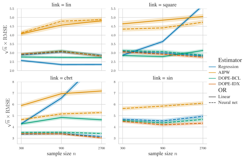
Figure 3. Root mean square errors for various estimators of $\chi_{1}$ plotted against sample size. Each data point is an average over 900 datasets, 300 for each choice of $d\in\{4,12,36\}$. The bands around each line correspond to $\pm 1$ standard error. For this plot, the outcome regression (OR) was fitted separately for each stratum $T=1$ and $T=2$.

The results for stratified outcome regression are shown in Figure 3. Each panel, corresponding to a link function in (22), displays the RMSE for various estimators against sample size. Across different values of $d\in\{4,12,36\}$, the results remain consistent, and thus the RMSE is averaged over the $3\times 300$ datasets with varying $d$. In the upper left panel, where the link is linear, the regression estimator $\widehat{\chi}_{1}^{\mathrm{reg}}$ with OLS performs best as expected. The remaining estimators exhibit similar performance, except for AIPW, which consistently performs poorly across all settings. This can be attributed to extreme values of the propensity score, resulting in a large efficiency bound for AIPW. All estimators seem to maintain an approximate $\sqrt{n}$-consistent RMSE for the linear link as anticipated.

For the nonlinear links, we observe that the OLS-based regression estimators perform poorly and do not exhibit approximate $\sqrt{n}$-consistency. For the sine link, the RMSEs for all OLS-based estimators are large, and they are not shown for ease of visualization. For neural network outcome regression, the AIPW still performs the worst across all nonlinear links. The regression estimator and the DOPE estimators share similar performance when used with the neural network, with DOPE-IDX being more accurate overall. Since the neural network architecture is tailored to the single-index model, it is not surprising that the outcome regression works well, and as a result there is less need for debiasing. On the other hand, the debiasing introduced in the DOPE does not hurt the accuracy, and in fact, improves it in this setting.

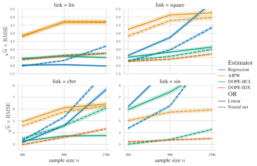
Figure 4. Root mean square errors for various estimators of $\chi_{1}$ plotted against sample size. Each data point is an average over 900 datasets, 300 for each choice of $d\in\{4,12,36\}$. The bands around each line correspond to $\pm 1$ standard error. For this plot, the outcome regression (OR) was fitted jointly onto $(T,\mathbf{W})$.

The results for joint regression of $Y$ on $(T,\mathbf{W})$ are shown in Figure 4. The results for the OLS-based estimators provide similar insights as previously discussed, so we focus on the results for the neural network based estimators. The jointly trained neural network is, in a sense, misspecified for the single-index model (except for the linear link), as discussed in Subsection 5.1.2. Thus it is not surprising that the regression estimator fails to adjust effectively for larger sample sizes. What is somewhat unexpected, however, is that the precision of DOPE, especially the DOPE-IDX, does not appear to be compromised by the misspecified outcome regression. In fact, the DOPE-IDX even seems to perform better with joint outcome regression. We suspect that this could be attributed to the joint regression producing more robust predictions for the rare treated subjects with $W^{1}\leq 0.5$, for which $m(1\,|\,\mathbf{W})=0.01$. The predictions are more robust since the joint regression can leverage some of the information from the many untreated subjects with $W^{1}\leq 0.5$ at the cost of introducing systematic bias, which the DOPE-IDX deals with in the debiasing step. While this phenomenon is interesting, a thorough exploration of its exact details, both numerically and theoretically, is a task we believe is better suited for future research.

In summary, the DOPE serves as a middle ground between the regression estimator and the AIPW. It provides an additional safeguard against biased outcome regression, all while avoiding the potential numerical instability entailed by using standard inverse propensity weights.

5.1.4. Inference

We now consider approximate confidence intervals obtained from the empirical variance estimator $\widehat{\mathcal{V}}$ defined in (17). Specifically, we consider intervals of the form $\widehat{\chi}_{1}\pm\frac{z_{0.975}}{\sqrt{n}}\widehat{\mathcal{V}}^{-1/2}$, where $z_{0.975}$ is the $0.975$ quantile of the standard normal distribution.

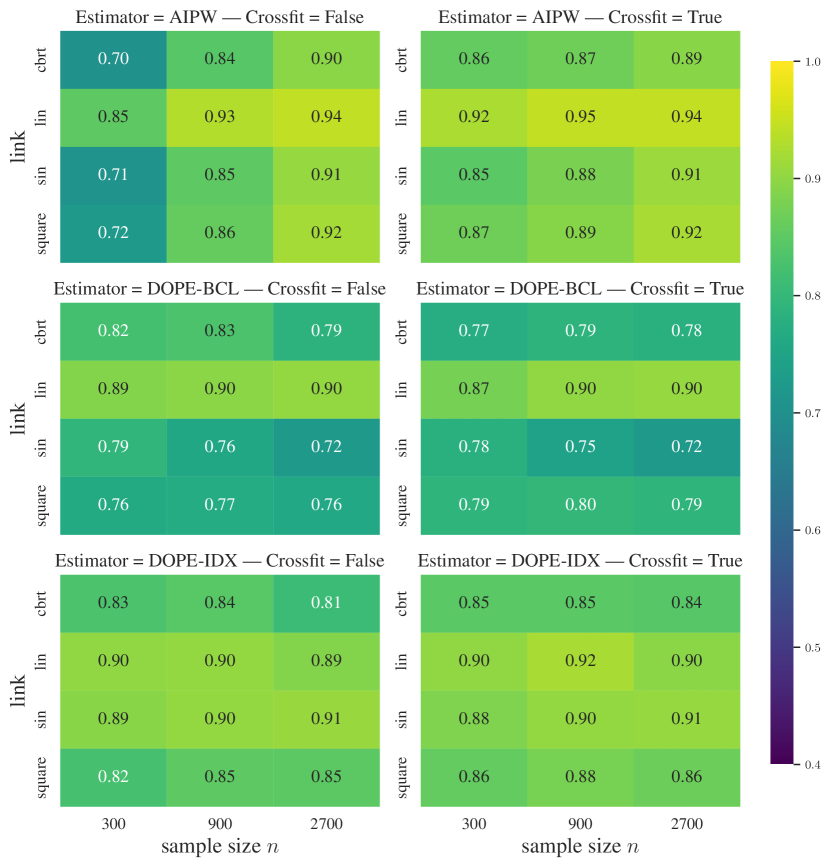
Figure 5. Coverage of asymptotic confidence intervals of the adjusted mean $\chi_{1}$, aggregated over $d\in\{4,12,36\}$ and with the true $\beta$ given in (5.1.1).

Figure 5 shows the empirical coverage of $\chi_{1}$ for the AIPW, DOPE-BCL and DOPE-IDX, all based on neural network outcome regression fitted jointly. Based on the number of repetitions, we can expect the estimated coverage probabilities to be accurate up to $\pm 0.01$ after rounding.

The left column shows the results for no sample splitting, whereas the right column shows the results for 4-fold cross-fitting. For all estimators, cross-fitting seems to improve coverage slightly for large sample sizes. The AIPW is a little anti-conservative, especially for the links $h_{\text{sin}}$ and $h_{\text{cbrt}}$, but overall maintains approximate coverage. The slight miscoverage is to be expected given the challenging nature with the extreme propensity weights. For the DOPE-BCL and DOPE-IDX, the coverage probabilities are worse, but with the DOPE-IDX having better coverage overall. According to our asymptotic analysis, specifically Theorem 4.3, the DOPE-BCL and DOPE-IDX intervals will only achieve asymptotic $95\%$ coverage of the random parameters $\chi_{1}(\widehat{h}(t,\mathbf{Z}_{\hat{\theta}}))$ and $\chi_{1}(\mathbf{Z}_{\hat{\theta}})$, respectively. Thus we do not anticipate these intervals to asymptotically achieve the nominal $95\%$ coverage of $\chi_{1}$. However, we show in Figure 9 in the supplementary Section B that the average widths of the confidence intervals are significantly smaller for the DOPE intervals than the AIPW interval. Hence it is possible that the DOPE intervals can be corrected – as we have also discussed in Remark 4.7 – to gain advantage over the AIPW interval, but we leave such explorations for future work.

In summary, the lack of full coverage for the naively constructed intervals are consistent with the asymptotic analysis conditionally on a representation $\mathbf{Z}_{\hat{\theta}}$. In view of this, our asymptotic results might be more realistic and pragmatic than the previously studied regime (Benkeser et al., 2020; Ju et al., 2020), which assumes fast unconditional rates of the nuisance parameters $(\widehat{m}_{\hat{\theta}},\widehat{g}_{\hat{\theta}})$.

5.2. Application to NHANES data

We consider the mortality dataset collected by the National Health and Nutrition Examination Survey I Epidemiologic Followup Study (Cox et al., 1997), henceforth referred to as the NHANES dataset. The dataset was initially collected as in Lundberg et al. (2020). The dataset contains several baseline covariates, and our outcome variable is the indicator of death at the end of study. To deal with missing values, we considered both a complete mean imputation as in Lundberg et al. (2020), or a trimmed dataset where covariates with more than $50\%$ of their values missing are dropped and the rest are mean imputed. The latter approach reduces the number of covariates from $79$ to $65$. The final results were similar for the two imputation methods, so we only report the results for the mean imputed dataset here. In the supplementary Section B we show the results for the trimmed dataset.

The primary aim of this section is to evaluate the different estimation methodologies on a realistic and real data example. For this purpose we consider a treatment variable based on pulse pressure and study its effect on mortality. Pulse pressure is defined as the difference between systolic and diastolic blood pressure (BP). High pulse pressure is not only used as an indicator of disease but is also reported to increase the risk of cardiovascular diseases (Franklin et al., 1999). We investigate the added effect of high pulse pressure when adjusting for other baseline covariates, in particular systolic BP and levels of white blood cells, hemoglobin, hematocrit, and platelets. We do not adjust for diastolic BP, as it determines the pulse pressure when combined with systolic BP, which would therefore lead to a violation of positivity.

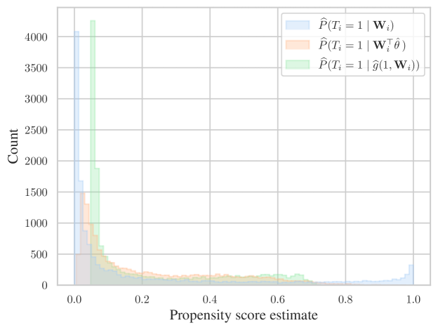
Figure 6. Distribution of estimated propensity scores based on the full covariate set $\mathbf{W}$, the single-index $\mathbf{W}^{\top}\hat{\theta}$, and the outcome predictions $\widehat{g}(1,\mathbf{W})$, respectively.

A pulse pressure of 40 mmHg is considered normal, and as the pressure increases past 50 mmHg, the risk of cardiovascular diseases is reported to increase. Some studies have used 60 mmHg as the threshold for high pulse pressure (Homan et al., 2024), and thus we consider the following treatment variable corresponding to high pulse pressure:

$$T=\mathbbl{1}\left(\textrm{pulse pressure}>60\textrm{ mmHg}\right).$$

For the binary outcome regression we consider logistic regression and a variant of the neural network from Section 5.1.2 with an additional ‘sigmoid-activation’ on the output layer. Based on 5-fold cross-validation, logistic regression yields a log-loss of $0.50$, whereas the neural network yields a log-loss of $0.48$ (smaller is better).

Figure 6 shows the distribution of the estimated propensity scores used in the AIPW, DOPE-IDX, and DOPE-BCL, based on neural network regression. As expected, we see that the full covariate set yields propensity scores that essentially violate positivity, with this effect being less pronounced for DOPE-IDX and even less so for DOPE-BCL, where the scores are comparatively less extreme.

Estimator	Estimate	BS se	BS CI
Regr. (NN)	0.022	0.009	(0.004, 0.037)
Naive contrast	0.388	0.010	(0.369, 0.407)
Regr. (Logistic)	0.026	0.010	(0.012, 0.049)
DOPE-BCL (Logistic)	0.023	0.010	(0.003, 0.040)
DOPE-BCL (NN)	0.021	0.010	(0.001, 0.039)
DOPE-IDX (NN)	0.024	0.012	(0.002, 0.048)
AIPW (NN)	0.023	0.015	(-0.009, 0.051)
AIPW (Logistic)	0.026	0.015	(-0.004, 0.056)
IPW (Logistic)	-0.040	0.025	(-0.103, -0.006)

Table 1. Adjusted effect estimates of unhealthy pulse pressure on mortality based on NHANES dataset. Estimators are sorted in increasing order after bootstrap (BS) standard error.

Table 1 shows the estimated treatment effects $\widehat{\Delta}=\widehat{\chi}_{1}-\widehat{\chi}_{0}$ for various estimators together with $95\%$ bootstrap confidence intervals. The estimators are sorted according to bootstrap variance based on $B=1000$ bootstraps. Because we do not know the true effect, we cannot directly decide which estimator is best. The naive contrast provides a substantially larger estimate than all of the adjustment estimators, which indicates that the added effect of high pulse pressure on mortality when adjusting is different from the unadjusted effect. The IPW estimator, $\widehat{\chi}_{1}^{\mathrm{ipw}}$, is the only estimator to yield a negative estimate of the adjusted effect, and its bootstrap variance is also significantly larger than the other estimators. Thus it is plausible, that the IPW estimator fails to adjust appropriately. This is not surprising given extreme distribution of the propensity weights, as shown in blue in Figure 6.

The remaining estimators yield comparable estimates of the adjusted effect, with the logistic regression based estimators having a marginally larger estimates than their neural network counterparts. The (bootstrap) standard errors are comparable for the DOPE and regression estimators, but the AIPW estimators have the slightly larger standard errors. As a result, the added effect of high pulse pressure on mortality cannot be considered statistically significant for the AIPW estimators, whereas it can for the other estimators.

In summary, the results indicate that the choice treatment effect estimator impacts the final estimate and confidence interval. While it is uncertain which estimator is superior for this particular application, the DOPE estimators seem to offer a reasonable and stable estimate.

6. Discussion

In this paper, we address challenges posed by complex data with unknown underlying structure, an increasingly common scenario in observational studies. Specifically, we have formulated a refined and general formalism for studying efficiency of covariate adjustment. This formalism extends and builds upon the efficiency principles derived from causal graphical models, in particular results provided by Rotnitzky & Smucler (2020). Our theoretical framework has led to the identification of the optimal covariate information for adjustment. From this theoretical groundwork, we introduced the DOPE for general estimation of the ATE with increased efficiency.

Several key areas within this research merit further investigation:

Extension to other targets and causal effects: Our focus has predominantly been on the adjusted mean $\chi_{t}=\mathbb{E}[\mathbb{E}[Y\,|\,T=t,\mathbf{W}]]$. However, the extension of our methodologies to continuous treatments, instrumental variables, or other causal effects, such as the average treatment effect among the treated, is an area that warrants in-depth exploration. We suspect that many of the fundamental ideas can be modified to prove analogous results for such target parameters.

Beyond neural networks: While our examples and simulation study has applied the DOPE with neural networks, its compatibility with other regression methods such as kernel regression and gradient boosting opens new avenues for alternative adjustment estimators. Investigating such estimators can provide practical insights and broaden the applicability of our approach. The Outcome Highly Adapted Lasso (Ju et al., 2020) is a similar method in this direction that leverages the Highly Adaptive Lasso (Benkeser & van der Laan, 2016) for robust treatment effect estimation.

Causal representation learning integration: Another possible direction for future research is the integration of our efficiency analysis into the broader concept of causal representation learning (Schölkopf et al., 2021). This line of research, which is not concerned with specific downstream tasks, could potentially benefit from some of the insights of our efficiency analysis and the DOPE framework.

Implications of sample splitting: Our current asymptotic analysis relies on the implementation of three distinct sample splits. Yet, our simulation results suggest that sample splitting might not be necessary. Using the notation of Algorithm 1, we hypothesize that the independence assumption $\mathcal{I}_{3}\cap(\mathcal{I}_{1}\cup\mathcal{I}_{2})=\emptyset$ could be replaced with Donsker class conditions. However, the theoretical justifications for setting $\mathcal{I}_{1}$ identical to $\mathcal{I}_{2}$ are not as evident, thus meriting additional exploration into this potential simplification.

Valid and efficient confidence intervals: The naive confidence intervals explored in the simulation study, cf. Section 5.1.4, do not provide an adequate coverage of the unconditional adjusted mean. As indicated in Remark 4.7, it would be interesting to explore methods for correcting the intervals, for example by: (i) adding a bias correction, (ii) constructing a consistent estimator of the unconditional variance, or (iii) using bootstrapping. Appealing to bootstrapping techniques, however, might be computationally expensive, in particular when combined with cross-fitting. To implement (i), one approach could be to generalize Theorem 4.6 to establish general differentiability of the adjusted mean with respect to general representations, and then construct an estimator of the gradient. However, one must asses whether this bias correction could negate the efficiency benefits of the DOPE.

Supplement to ‘Efficient adjustment for complex covariates: Gaining efficiency with DOPE’

The supplementary material is organized as follows: Section A contains proofs of the results in the main text and a few auxiliary results; Section B contains details on the experiments in Section 5; and Section C contains a description of the cross-fitting algorithm.

Appendix A Auxiliary results and proofs

The proposition below relaxes the criteria for being a valid adjustment set in a causal graphical model. It follows from the results of Perković et al. (2018), which was pointed out to the authors by Leonard Henckel, and is stated here for completeness.

Proposition A.1.

Let $T,\mathbf{Z}$, and $Y$ be pairwise disjoint node sets in a DAG $\mathcal{D}=(\mathbf{V},\mathbf{E})$, and let $\mathcal{M}(\mathcal{D})$ denote the collection of continuous distributions that are Markovian with respect to $\mathcal{D}$ and with $\mathbb{E}|Y|<\infty$. Then $\mathbf{Z}$ is an adjustment set relative to $(T,Y)$ if and only if for all $P\in\mathcal{M}(\mathcal{D})$ and all $t$

$$\mathbb{E}_{P}[Y\,|\,\mathrm{do}(T=t)]=\mathbb{E}_{P}\left[\frac{\mathbbl{1}(T=t)Y}{\mathbb{P}_{P}(T=t\,|\,\mathrm{pa}_{\mathcal{D}}(T))}\right]=\mathbb{E}_{P}[\mathbb{E}_{P}[Y\,|\,T=t,\mathbf{Z}]]$$

Proof.

The ‘only if’ direction is straightforward if we use an alternative characterization of $\mathbf{Z}$ being an adjustment set: for any density $p$ of a distribution $P\in\mathcal{P}$ it holds that

$$p(y\,|\,\mathrm{do}(T=t))=\int p(\mathbf{y}|\mathbf{z},t)p(\mathbf{z})\mathrm{d}\mathbf{z},$$

where the ‘do-operator’ (and notation) is defined as in, e.g., Peters et al. (2017). Dominated convergence then yields

$$\mathbb{E}_{P}[Y\,|\,\mathrm{do}(T=t)] =\mathbb{E}_{P}[\mathbb{E}_{P}[Y\,|\,T=t,\mathbf{Z}]],$$

which is equivalent to the ‘only if’ part. On the contrary, assume that $\mathbf{Z}$ is not an adjustment set for $(T,Y)$. Then Theorem 56 and the proof of Theorem 57 in Perković et al. (2018) imply the existence of a Gaussian distribution $\tilde{P}\in\mathcal{P}$ for which

$$\mathbb{E}_{\tilde{P}}[Y\,|\,\mathrm{do}(T=1)]\neq\mathbb{E}_{\tilde{P}}[\mathbb{E}_{\tilde{P}}[Y\,|\,T=1,\mathbf{Z}]]$$

This implies the other direction. ∎

The following lemma is a generalization of Lemma 27 in Rotnitzky & Smucler (2020).

Lemma A.2.

For any $\sigma$-algebras $\mathcal{Z}_{1}\subseteq\mathcal{Z}_{2}\subseteq\sigma(\mathbf{W})$ it holds, under Assumption 1.1, that

$$\mathbb{E}_{P}\left[\pi_{t}(\mathcal{Z}_{2};P)^{-1}\,|\,T=t,\mathcal{Z}_{1}\right]=\pi_{t}(\mathcal{Z}_{1};P)^{-1}$$

for all $P\in\mathcal{P}$.

Proof.

Direct computation yields

$$\mathbb{E}_{P}\left[\pi_{t}(\mathcal{Z}_{2};P)^{-1}\,|\,T=t,\mathcal{Z}_{1}\right]\mathbb{P}_{P}(T=t\,|\,\mathcal{Z}_{1})$$

$$=\mathbb{E}_{P}\left[\frac{\mathbbl{1}(T=t)}{\pi_{t}(\mathcal{Z}_{2};P)}\,|\,\mathcal{Z}_{1}\right]=\mathbb{E}_{P}\left[\frac{\mathbb{E}_{P}[\mathbbl{1}(T=t)\,|\,\mathcal{Z}_{2}]}{\pi_{t}(\mathcal{Z}_{2};P)}\,|\,\mathcal{Z}_{1}\right]=1.$$

∎

A.1. Proof of Lemma 3.1

Since $P\in\mathcal{P}$ is fixed, we suppress it from the notation in the following computations.

From $Y\,\perp\!\!\!\perp\,\mathcal{Z}_{2}\,|\,\mathcal{Z}_{1},T$ and $\mathcal{Z}_{1}\subseteq\mathcal{Z}_{2}$, it follows that $\mathbb{E}[Y\,|\,\mathcal{Z}_{1},T]=\mathbb{E}[Y\,|\,\mathcal{Z}_{2},T]$. Hence, for each $t\in\mathbb{T}$,

(23) $$b_{t}(\mathcal{Z}_{1})=\mathbb{E}[Y\,|\,\mathcal{Z}_{1},T=t]=\mathbb{E}[Y\,|\,\mathcal{Z}_{2},T=t]=b_{t}(\mathcal{Z}_{2}).$$

Therefore $\chi_{t}(\mathcal{Z}_{1})=\mathbb{E}[b_{t}(\mathcal{Z}_{1})]=\mathbb{E}[b_{t}(\mathcal{Z}_{2})]=\chi_{t}(\mathcal{Z}_{2})$. If $\mathcal{Z}_{2}$ is description of $\mathbf{W}$, this identity shows that $\mathcal{Z}_{2}$ is $\mathcal{P}$-valid if and only if $\mathcal{Z}_{1}$ is $\mathcal{P}$-valid.

To compare the asymptotic efficiency bounds for $\mathcal{Z}_{2}$ with $\mathcal{Z}_{1}$ we use the law of total variance. Note first that

$$\mathbb{E}[\psi_{t}(\mathcal{Z}_{2})\,|\,T,Y,\mathcal{Z}_{1}] =\mathbb{E}\Big{[}\mathbbl{1}(T=t)(Y-b_{t}(\mathcal{Z}_{2}))\frac{1}{\pi_{t}(\mathcal{Z}_{2})}+b_{t}(\mathcal{Z}_{2})-\chi_{t}\,|\,T,Y,\mathcal{Z}_{1}\Big{]}$$

$$=\mathbbl{1}(T=t)(Y-b_{t}(\mathcal{Z}_{1}))\,\mathbb{E}\Big{[}\frac{1}{\pi_{t}(\mathcal{Z}_{2})}\,|\,T=t,Y,\mathcal{Z}_{1}\Big{]}+b_{t}(\mathcal{Z}_{1})-\chi_{t}$$

$$=\mathbbl{1}(T=t)(Y-b_{t}(\mathcal{Z}_{1}))\mathbb{E}\left[\frac{1}{\pi_{t}(\mathcal{Z}_{2})}\,|\,T=t,\mathcal{Z}_{1}\right]+b_{t}(\mathcal{Z}_{1})-\chi_{t}$$

$$=\mathbbl{1}(T=t)(Y-b_{t}(\mathcal{Z}_{1}))\frac{1}{\pi_{t}(\mathcal{Z}_{1})}+b_{t}(\mathcal{Z}_{1})-\chi_{t}=\psi_{t}(\mathcal{Z}_{1}).$$

Second equality is due to $\mathcal{Z}_{1}$-measurability and (23), whereas the third equality follows from $Y\,\perp\!\!\!\perp\,\mathcal{Z}_{2}\,|\,\mathcal{Z}_{1},T$ and the last inequality is due to Lemma A.2. On the other hand,

$$\phantom{=}\mathbb{E}\big{[}\operatorname{Var}(\psi_{t}(\mathcal{Z}_{2})\,|\,T,Y,\mathcal{Z}_{1})\big{]}$$

$$=\mathbb{E}\Big{[}\operatorname{Var}\Big{(}\mathbbl{1}(T=t)(Y-b_{t}(\mathcal{Z}_{1}))\frac{1}{\pi_{t}(\mathcal{Z}_{2})}+b_{t}(\mathcal{Z}_{1})-\chi_{t}(P)\;\big{|}\;T,Y,\mathcal{Z}_{1}\Big{)}\Big{]}$$

$$=\mathbb{E}\Big{[}\mathbbl{1}(T=t)(Y-b_{t}(\mathcal{Z}_{1}))^{2}\operatorname{Var}\Big{(}\frac{1}{\pi_{t}(\mathcal{Z}_{2})}\;\big{|}\;T=t,Y,\mathcal{Z}_{1}\Big{)}\Big{]}$$

$$=\mathbb{E}\Big{[}\pi_{t}(\mathcal{Z}_{1})\operatorname{Var}(Y\,|\,T=t,\mathcal{Z}_{1})\operatorname{Var}\Big{(}\frac{1}{\pi_{t}(\mathcal{Z}_{2})}\;\big{|}\;T=t,\mathcal{Z}_{1}\Big{)}\Big{]}.$$

Combined we have that

$$\mathbb{V}_{t}(\mathcal{Z}_{2}) =\operatorname{Var}(\psi_{t}(\mathcal{Z}_{2}))=\operatorname{Var}(\mathbb{E}[\psi_{t}(\mathcal{Z}_{2})\,|\,T,Y,\mathcal{Z}_{1}])+\mathbb{E}[\operatorname{Var}[\psi_{t}(\mathcal{Z}_{2})\,|\,T,Y,\mathcal{Z}_{1}]]$$

$$=\mathbb{V}_{t}(\mathcal{Z}_{1})+\mathbb{E}\Big{[}\pi_{t}(\mathcal{Z}_{1})\operatorname{Var}(Y\,|\,T=t,\mathcal{Z}_{1})\operatorname{Var}\Big{(}\frac{1}{\pi_{t}(\mathcal{Z}_{2})}\Big{|}\;T=t,Y,\mathcal{Z}_{1}\Big{)}\Big{]}.$$

To prove the last part of the lemma, we first note that $\psi_{t}(\mathcal{Z}_{2})$ and $\psi_{t^{\prime}}(\mathcal{Z}_{2})$ are conditionally uncorrelated for $t\neq t^{\prime}$. This follows from (23), from which the conditional covariance reduces to

$$\operatorname{Cov}(\psi_{t}(\mathcal{Z}_{2}),\psi_{t^{\prime}}(\mathcal{Z}_{2})\,|\,T,Y,\mathcal{Z}_{1})=\mathbbl{1}(T=t)\mathbbl{1}(T=t^{\prime})\operatorname{Cov}(*,*\,|\,T,Y,\mathcal{Z}_{1})=0.$$

Thus, letting $\psi(\mathcal{Z}_{2})=(\psi_{t}(\mathcal{Z}_{2}))_{t\in\mathbb{T}}$ and using the computation for $\mathbb{V}_{t}$, we obtain that:

$$\mathbb{V}_{\Delta}(\mathcal{Z}_{2})=\operatorname{Var}(\mathbf{c}^{\top}\psi(\mathcal{Z}_{2}))$$

$$=\operatorname{Var}(\mathbb{E}[\mathbf{c}^{\top}\psi(\mathcal{Z}_{2})\,|\,T,Y,\mathcal{Z}_{1}])+\mathbb{E}[\operatorname{Var}[\mathbf{c}^{\top}\psi(\mathcal{Z}_{2})\,|\,T,Y,\mathcal{Z}_{1}]]$$

$$=\mathbb{V}_{\Delta}(\mathcal{Z}_{1})+\sum_{t\in\mathbb{T}}c_{t}^{2}\,\mathbb{E}\Big{[}\pi_{t}(\mathcal{Z}_{1})\operatorname{Var}(Y\,|\,T=t,\mathcal{Z}_{1})\operatorname{Var}\Big{(}\frac{1}{\pi_{t}(\mathcal{Z}_{2})}\Big{|}\;T=t,Y,\mathcal{Z}_{1}\Big{)}\Big{]}.$$

This concludes the proof. ∎

A.2. Proof of Theorem 3.3

(i) Assume that $\mathcal{Z}\subseteq\sigma(\mathbf{W})$ is a description of $\mathbf{W}$ such that $\mathcal{Q}_{P}\subseteq\overline{\mathcal{Z}}$. Observe that almost surely,

$$\mathbb{P}_{P}(Y\leq y\,|\,T,\mathbf{W})=\sum_{t\in\mathbb{T}}\mathbbl{1}(T=t)F(y\mid t,\mathbf{W};P)$$

is $\sigma(T,\mathcal{Q}_{P})$-measurable and hence also $\sigma(T,\overline{\mathcal{Z}})$-measurable. It follows that $\mathbb{P}_{P}(Y\leq y\,|\,T,\mathbf{W})$ is also a version of $\mathbb{P}_{P}(Y\leq y\,|\,T,\overline{\mathcal{Z}})$. As a consequence, $\mathbb{P}_{P}(Y\leq y\,|\,T,\mathbf{W})=\mathbb{P}_{P}(Y\leq y\,|\,T,\mathcal{Z})$ almost surely. From Doob’s characterization of conditional independence (Kallenberg 2021, Theorem 8.9), we conclude that $Y\,{\perp\!\!\!\perp}_{P}\,\mathbf{W}\mid T,\mathcal{Z}$, or equivalently that $\mathcal{Z}$ is $P$-ODS. The ‘in particular’ follows from setting $\mathcal{Z}=\mathcal{Q}_{P}$.

(ii) Assume that $\mathcal{Z}\subseteq\sigma(\mathbf{W})$ is $P$-ODS. Using Doob’s characterization of conditional independence again, $\mathbb{P}_{P}(Y\leq y\,|\,T,\mathbf{W})=\mathbb{P}_{P}(Y\leq y\,|\,T,\mathcal{Z})$ almost surely. Under Assumption 1.1, this entails that $F(y\,|\,T=t,\mathbf{W};P)=\mathbb{P}_{P}(Y\leq y\,|\,T=t,\mathcal{Z})$ almost surely, and hence $F(y\,|\,T=t,\mathbf{W};P)$ must be $\overline{\mathcal{Z}}$-measurable. As the generators of $\mathcal{Q}_{P}$ are $\overline{\mathcal{Z}}$-measurable, we conclude that $\mathcal{Q}_{P}\subseteq\overline{\mathcal{Z}}$.

(iii) Let $\mathcal{Z}$ be a $P$-ODS description. From (i) and (ii) it follows that $\mathcal{Q}_{P}\subseteq\overline{\mathcal{Z}}$, and since $\mathcal{Z}\subseteq\sigma(\mathbf{W})$ it also holds that $Y\,{\perp\!\!\!\perp}_{P}\,\overline{\mathcal{Z}}\mid T,\mathcal{Q}_{P}$. Since $\mathbb{V}_{\Delta}(\mathcal{Z};P)=\mathbb{V}_{\Delta}(\overline{\mathcal{Z}};P)$, Lemma 3.1 gives the desired conclusion. ∎

A.3. Proof of Corollary 3.4

Theorem 3.3 (i,ii) implies that $\mathcal{Z}$ is $\mathcal{P}$-ODS if and only if $\overline{\mathcal{Z}}^{P}$ contains $\mathcal{Q}_{P}$ for all $P\in\mathcal{P}$.

If $\mathcal{Q}\subseteq\overline{\mathcal{Z}}^{P}$ for all $P\in\mathcal{P}$ then $\mathcal{Q}_{P}\subseteq\overline{\mathcal{Z}}^{P}$ for all $P\in\mathcal{P}$ by definition, and $\mathcal{Z}$ is $\mathcal{P}$-ODS. Equation (9) follows from the same argument as Theorem 3.3 $(iii)$. That is, $\mathcal{Q}\subseteq\overline{\mathcal{Z}}^{P}$, and since $\mathcal{Q}$ is $P$-ODS and $\mathcal{Z}\subseteq\sigma(\mathbf{W})$ we have $Y\,{\perp\!\!\!\perp}_{P}\,\overline{\mathcal{Z}}^{P}\mid T,\mathcal{Q}$. Lemma 3.1 can be applied for each $P\in\mathcal{P}$ to obtain the desired conclusion. ∎

A.4. Proof of Proposition 3.6

Since $\mathcal{R}_{P}\subseteq\mathcal{Q}_{P}$ always holds, so it suffices to prove that $\mathcal{Q}_{P}\subseteq\mathcal{R}_{P}$. If $F(y\,|\,t,\mathbf{W};P)$ is $\sigma(b_{t}(\mathbf{W};P))$-measurable, then $\mathcal{Q}_{P}\subseteq\mathcal{R}_{P}$ follows directly from definition. If $Y$ is a binary outcome, then the conditional distribution is determined by the conditional mean, i.e., $F(y\,|\,t,\mathbf{W};P)$ is $\sigma(b_{t}(\mathbf{W};P))$-measurable. If $Y=b_{T}(\mathbf{W})+\varepsilon_{Y}$ with $\varepsilon_{Y}\,\perp\!\!\!\perp\,T,\mathbf{W}$, then $F(y\,|\,t,\mathbf{w};P)=F_{P}(y-b_{t}(\mathbf{w}))$ where $F_{P}$ is the distribution function for the distribution of $\varepsilon_{Y}$. Again, $F(y\,|\,t,\mathbf{W};P)$ becomes $\sigma(b_{t}(\mathbf{W};P))$-measurable.

To prove the last part, let $\mathcal{Z}$ be a $P$-OMS description. Since $b_{t}(\mathbf{W};P)=b_{t}(\mathcal{Z};P)$ is $\mathcal{Z}$-measurable for every $t\in\mathbb{T}$, it follows that $\mathcal{R}_{P}\subseteq\overline{\mathcal{Z}}$. Hence the argument of Theorem 3.3 $(iii)$ establishes Equation (8) when $\mathcal{Q}_{P}=\mathcal{R}_{P}$. ∎

A.5. Proof of Lemma 3.8

Since $P\in\mathcal{P}$ is fixed throughout this proof, we suppress it from notation. From $\mathcal{Z}_{1}\subseteq\mathcal{Z}_{2}\subseteq\sigma(\mathbf{W})$ and $T\,{\perp\!\!\!\perp}_{P}\,\mathcal{Z}_{2}\,|\,\mathcal{Z}_{1}$, it follows that $\pi_{t}(\mathcal{Z}_{1})=\pi_{t}(\mathcal{Z}_{1})$, and hence

$$\chi_{t}(\mathcal{Z}_{1})=\mathbb{E}[\pi_{t}(\mathcal{Z}_{1})^{-1}\mathbbl{1}(T=t)Y]=\mathbb{E}[\pi_{t}(\mathcal{Z}_{2})^{-1}\mathbbl{1}(T=t)Y]=\chi_{t}(\mathcal{Z}_{2}).$$

This establishes the first part. For the second part, we use that $\pi_{t}(\mathcal{Z}_{1})=\pi_{t}(\mathcal{Z}_{2})$ and $\chi_{t}(\mathcal{Z}_{1})=\chi_{t}(\mathcal{Z}_{2})$ to see that

$$\psi_{t}(\mathcal{Z}_{1})-\psi_{t}(\mathcal{Z}_{2}) =b_{t}(\mathcal{Z}_{1})-b_{t}(\mathcal{Z}_{2})+\frac{\mathbbl{1}(T=t)}{\pi_{t}(\mathcal{Z}_{2})}(b_{t}(\mathcal{Z}_{2})-b_{t}(\mathcal{Z}_{1}))$$

$$=\Big{(}\frac{\mathbbl{1}(T=t)}{\pi_{t}(\mathcal{Z}_{2})}-1\Big{)}(b_{t}(\mathcal{Z}_{2})-b_{t}(\mathcal{Z}_{1}))\eqcolon R_{t}(\mathcal{Z}_{1},\mathcal{Z}_{2}).$$

Since $\mathbb{E}[R_{t}(\mathcal{Z}_{1},\mathcal{Z}_{2})\,|\,\mathcal{Z}_{2}]=0$ we have that $\mathbb{E}[\psi_{t}(\mathcal{Z}_{2})R_{t}(\mathcal{Z}_{1},\mathcal{Z}_{2})]=0$, which means that $\psi_{t}(\mathcal{Z}_{2})$ and $R_{t}(\mathcal{Z}_{1},\mathcal{Z}_{2})$ are uncorrelated. Note that from $\pi_{t}(\mathcal{Z}_{1})=\pi_{t}(\mathcal{Z}_{2})$ it also follows that

$$b_{t}(\mathcal{Z}_{1})=\mathbb{E}\Big{[}\frac{Y\mathbbl{1}(T=t)}{\pi_{t}(\mathcal{Z}_{1})}\,|\,\mathcal{Z}_{1}\Big{]}=\mathbb{E}\Big{[}\mathbb{E}\Big{[}\frac{Y\mathbbl{1}(T=t)}{\pi_{t}(\mathcal{Z}_{2})}\,|\,\mathcal{Z}_{2}\Big{]}\,|\,\mathcal{Z}_{1}\Big{]}=\mathbb{E}[b_{t}(\mathcal{Z}_{2})\,|\,\mathcal{Z}_{1}]$$

This means that $\mathbb{E}[(b_{t}(\mathcal{Z}_{2})-b_{t}(\mathcal{Z}_{1}))^{2}\,|\,\mathcal{Z}_{1}]=\operatorname{Var}(b_{t}(\mathcal{Z}_{2})\,|\,\mathcal{Z}_{1})$. These observations let us compute that

$$\mathbb{V}_{t}(\mathcal{Z}_{1}) =\operatorname{Var}(\psi_{t}(\mathcal{Z}_{1}))$$

$$=\operatorname{Var}(\psi_{t}(\mathcal{Z}_{2}))+\operatorname{Var}\left(R_{t}(\mathcal{Z}_{1},\mathcal{Z}_{2})\right)$$

$$=\operatorname{Var}(\psi_{t}(\mathcal{Z}_{2}))+\mathbb{E}[\mathbb{E}[R_{t}(\mathcal{Z}_{1},\mathcal{Z}_{2})^{2}\,|\,\mathcal{Z}_{2}]]$$

$$=\mathbb{V}_{t}(\mathcal{Z}_{2})+\mathbb{E}\Big{[}(b_{t}(\mathcal{Z}_{2})-b_{t}(\mathcal{Z}_{1}))^{2}\mathbb{E}\Big{[}\frac{\mathbbl{1}(T=t)^{2}}{\pi_{t}(\mathcal{Z}_{1})^{2}}-\frac{2\mathbbl{1}(T=t)}{\pi_{t}(\mathcal{Z}_{1})}+1\,|\,\mathcal{Z}_{2}\Big{]}\Big{]}$$

(24) $$=\mathbb{V}_{t}(\mathcal{Z}_{2})+\mathbb{E}\Big{[}\operatorname{Var}(b_{t}(\mathcal{Z}_{2})\,|\,\mathcal{Z}_{1})\Big{(}\frac{1}{\pi_{t}(\mathcal{Z}_{1})}-1\Big{)}\Big{]}.$$

This establishes the formula in the case $\Delta=\chi_{t}$.

For general $\Delta$, note first that $\mathbf{R}$ and $(\psi_{t}(\mathcal{Z}_{2}))_{t\in\mathbb{T}}$ are uncorrelated since $\mathbb{E}[\mathbf{R}\,|\,\mathcal{Z}_{2}]=0$. Therefore we have

$$\mathbb{V}_{\!\Delta}(\mathcal{Z}_{1}) =\operatorname{Var}\Big{(}\sum_{t\in\mathbb{T}}c_{t}\psi_{t}(\mathcal{Z}_{1})\Big{)}$$

$$=\operatorname{Var}\Big{(}\sum_{t\in\mathbb{T}}c_{t}\psi_{t}(\mathcal{Z}_{2})\Big{)}+\operatorname{Var}\Big{(}\sum_{t\in\mathbb{T}}c_{t}R_{t}(\mathcal{Z}_{1},\mathcal{Z}_{2})\Big{)}$$

$$=\mathbb{V}_{\!\Delta}(\mathcal{Z}_{2})+\mathbf{c}^{\top}\operatorname{Var}\Big{(}\mathbf{R}\Big{)}\mathbf{c}.$$

It now remains to establish the covariance expressions for the last term, since the expression of $\operatorname{Var}\left(R_{t}(\mathcal{Z}_{1},\mathcal{Z}_{2})\right)$ was found in (A.5). To this end, note first that for any $s,t\in\mathbb{T}$ with $s\neq t$,

$$\mathbb{E}\left[\Big{(}\frac{\mathbbl{1}(T=s)}{\pi_{s}(\mathcal{Z}_{2})}-1\Big{)}\Big{(}\frac{\mathbbl{1}(T=t)}{\pi_{t}(\mathcal{Z}_{2})}-1\Big{)}\,|\,\mathcal{Z}_{2}\right]=-1.$$

Thus we finally conclude that

$$\operatorname{Cov}(R_{s},R_{t}) =-\mathbb{E}\left[(b_{s}(\mathcal{Z}_{2})-b_{s}(\mathcal{Z}_{1}))(b_{t}(\mathcal{Z}_{2})-b_{t}(\mathcal{Z}_{1}))\right]$$

$$=-\mathbb{E}\left[\operatorname{Cov}(b_{s}(\mathcal{Z}_{2}),b_{t}(\mathcal{Z}_{2})\,|\,\mathcal{Z}_{1})\right],$$

as desired. ∎

A.6. Computations for Example 3.10

Using symmetry, we see that

$$\pi_{1}(\mathbf{Z}) =\mathbb{E}[T\mid\mathbf{Z}]=\mathbb{E}[\mathbf{W}\mid\mathbf{Z}]$$

$$=(0.5-\mathbf{Z})\mathbb{P}(\mathbf{W}\leq 0.5\,|\,\mathbf{Z})+(0.5+\mathbf{Z})\mathbb{P}(\mathbf{W}>0.5\,|\,\mathbf{Z})\ =\frac{1}{2}.$$

From $T\,\perp\!\!\!\perp\,\mathbf{Z}$ we observe that

$$b_{t}(\mathbf{W}) =t+\mathbb{E}[g(\mathbf{Z})\,|\,T=t,\mathbf{W}]=t+g(\mathbf{Z}),$$

$$b_{t}(\mathbf{Z}) =t+\mathbb{E}[g(\mathbf{Z})\,|\,T=t,\mathbf{Z}]=t+g(\mathbf{Z}),$$

$$b_{t}(0) =t+\mathbb{E}[g(\mathbf{Z})\,|\,T=t]=t+\mathbb{E}[g(\mathbf{Z})].$$

Plugging these expressions into the asymptotic variance yields:

$$\mathbb{V}_{t}(0) =\operatorname{Var}\left(b_{t}(0)+\frac{\mathbbl{1}(T=t)}{\pi_{t}(0)}(Y-b_{t}(0))\right)$$

$$=\pi_{t}(0)^{-2}\operatorname{Var}\left(\mathbbl{1}(T=t)(Y-b_{t}(0))\right)$$

$$=4\mathbb{E}[\mathbbl{1}(T=t)(g(\mathbf{Z})-\mathbb{E}[g(\mathbf{Z})]+v(\mathbf{W})\varepsilon_{Y})^{2}]$$

$$=4\mathbb{E}[\mathbf{W}(g(\mathbf{Z})-\mathbb{E}[g(\mathbf{Z})])^{2}]+2\mathbb{E}[v(\mathbf{W})\varepsilon_{Y}^{2}]$$

$$=2\operatorname{Var}(g(\mathbf{Z}))+2\mathbb{E}[v(\mathbf{W})^{2}]\mathbb{E}[\varepsilon_{Y}^{2}]$$

$$\mathbb{V}_{t}(\mathbf{Z}) =\operatorname{Var}\left(b_{t}(\mathbf{Z})+\frac{\mathbbl{1}(T=t)}{\pi_{t}(\mathbf{Z})}(Y-b_{t}(\mathbf{Z}))\right)$$

$$=\operatorname{Var}\left(g(\mathbf{Z})+2\mathbbl{1}(T=t)v(\mathbf{W})\varepsilon_{Y}\right)$$

$$=\operatorname{Var}\left(g(\mathbf{Z})\right)+2\mathbb{E}[v(\mathbf{W})^{2}]\mathbb{E}[\varepsilon_{Y}^{2}]$$

$$\mathbb{V}_{t}(\mathbf{W}) =\operatorname{Var}\left(b_{t}(\mathbf{W})+\frac{\mathbbl{1}(T=t)}{\pi_{t}(\mathbf{W})}(Y-b_{t}(\mathbf{W}))\right)$$

$$=\operatorname{Var}\left(g(\mathbf{Z})+\frac{\mathbbl{1}(T=t)v(\mathbf{W})\varepsilon_{Y}}{\mathbf{W}}\right)$$

$$=\operatorname{Var}\left(g(\mathbf{Z})\right)+\mathbb{E}\left[\frac{v(\mathbf{W})^{2}}{\mathbf{W}}\right]\mathbb{E}[\varepsilon_{Y}^{2}].$$

∎

Proof of Theorem 4.3

We first prove that $R_{i}\xrightarrow{P}0$ for $i=1,2,3$. The third term is taken care of by combining Assumption 4.2 (i,iv) with Cauchy-Schwarz:

$$|R_{3}| \leq\sqrt{|\mathcal{I}_{3}|}\sqrt{\frac{1}{|\mathcal{I}_{3}|}\sum_{i\in\mathcal{I}_{3}}\big{(}\widehat{m}_{\hat{\theta}}(t\,|\,\mathbf{W}_{i})^{-1}-m_{\hat{\theta}}(t\,|\,\mathbf{W}_{i})^{-1}\big{)}^{2}}\sqrt{\mathcal{E}_{2,t}^{(n)}}$$

$$\leq\ell_{c}\sqrt{|\mathcal{I}_{3}|\mathcal{E}_{1,t}^{(n)}\mathcal{E}_{2,t}^{(n)}}\xrightarrow{P}0,$$

where $\ell_{c}>0$ is the Lipschitz constant of $x\mapsto x^{-1}$ on $[c,1-c]$.

For the first term, $R_{1}$, note that conditionally on $\hat{\theta}$ and the observed estimated representations $\mathbf{Z}_{\hat{\bullet}}\coloneq(\mathbf{Z}_{\hat{\theta},i})_{i\in\mathcal{I}_{3}}=(\varphi(\hat{\theta},\mathbf{W}_{i}))_{i\in\mathcal{I}_{3}}$, the summands are conditionally i.i.d. due to Assumption 4.1. They are also conditionally mean zero since

$$\mathbb{E}[r_{i}^{1}\,|\,\mathbf{Z}_{\hat{\bullet}},\hat{\theta}\,] =\left(\widehat{g}_{\hat{\theta}}(t,\mathbf{W}_{i})-g_{\hat{\theta}}(t,\mathbf{W}_{i})\right)\Big{(}1-\frac{\mathbb{E}[\mathbbl{1}(T_{i}=t)\,|\,\mathbf{Z}_{\hat{\bullet}},\hat{\theta}\,]}{m_{\hat{\theta}}(t\,|\,\mathbf{W}_{i})}\Big{)}$$

$$=\left(\widehat{g}_{\hat{\theta}}(t,\mathbf{W}_{i})-g_{\hat{\theta}}(t,\mathbf{W}_{i})\right)\Big{(}1-\frac{\mathbb{E}[\mathbbl{1}(T_{i}=t)\,|\,\mathbf{Z}_{\hat{\theta},i},\hat{\theta}]}{m_{\hat{\theta}}(t\,|\,\mathbf{W}_{i})}\Big{)}=0,$$

for each $i\in\mathcal{I}_{3}$. Using Assumption 4.2 (i), we can bound the conditional variance by

$$\operatorname{Var}\left(r_{i}^{1}\,|\,\mathbf{Z}_{\hat{\bullet}},\hat{\theta}\,\right) =\frac{\left(\widehat{g}_{\hat{\theta}}(t,\mathbf{W}_{i})-g_{\hat{\theta}}(t,\mathbf{W}_{i})\right)^{2}}{m_{\hat{\theta}}(t\,|\,\mathbf{W})^{2}}\operatorname{Var}\left(\mathbbl{1}(T=t)\,|\,\mathbf{Z}_{\hat{\bullet}},\hat{\theta}\right)$$

$$=\frac{\left(\widehat{g}_{\hat{\theta}}(t,\mathbf{W}_{i})-g_{\hat{\theta}}(t,\mathbf{W}_{i})\right)^{2}}{m_{\hat{\theta}}(t\,|\,\mathbf{W})}(1-m_{\hat{\theta}}(t\,|\,\mathbf{W}))$$

$$\leq\frac{(1-c)}{c}\left(\widehat{g}_{\hat{\theta}}(t,\mathbf{W}_{i})-g_{\hat{\theta}}(t,\mathbf{W}_{i})\right)^{2}$$

Now it follows from Assumption 4.2 v and the conditional Chebyshev inequality that

$$\mathbb{P}\left(|R_{1}|>\epsilon\,|\,\mathbf{Z}_{\hat{\bullet}},\hat{\theta}\,\right) \leq\epsilon^{-2}\operatorname{Var}(R_{1}\,|\,\mathbf{Z}_{\hat{\bullet}},\hat{\theta})\leq\frac{1-c}{\epsilon^{2}c}\mathcal{E}_{2,t}^{(n)}\xrightarrow{P}0,$$

from which we conclude that $R_{1}\xrightarrow{P}0$.

The analysis of $R_{2}$ is similar. Observe that the summands are conditionally i.i.d. given $\mathbf{Z}_{\hat{\bullet}},\hat{\theta}$, and $T_{\bullet}\coloneq(T_{i})_{i\in\mathcal{I}_{3}}$. They are also conditionally mean zero since

$$\mathbb{E}\left[r_{i}^{2}\,|\,\mathbf{Z}_{\hat{\bullet}},T_{\bullet},\hat{\theta}\right]=\left(\mathbb{E}[Y_{i}\,|\,\mathbf{Z}_{\hat{\bullet}},T_{\bullet},\hat{\theta}]-g_{\hat{\theta}}(t,\mathbf{W}_{i})\right)\left(\frac{\mathbbl{1}(T_{i}=t)}{\widehat{m}_{\hat{\theta}}(\mathbf{W}_{i})}-\frac{\mathbbl{1}(T_{i}=t)}{m_{\hat{\theta}}(\mathbf{W}_{i})}\right)=0,$$

where we use that on the event $(T_{i}=t)$,

$$\mathbb{E}[Y_{i}\,|\,\mathbf{Z}_{\hat{\theta},i},T_{i},\hat{\theta}\,]=\mathbb{E}[Y_{i}\,|\,\mathbf{Z}_{\hat{\theta},i},T_{i}=t,\hat{\theta}\,]=g_{\hat{\theta}}(t,\mathbf{W}_{i}).$$

To bound the conditional variance, note first that Assumption 4.1 and Assumption 4.2 ii imply

$$\operatorname{Var}\big{(}Y_{i}\,|\,\mathbf{Z}_{\hat{\theta},i},T_{i},\hat{\theta}\,\big{)}\leq\mathbb{E}\big{[}Y_{i}^{2}\,|\,\mathbf{Z}_{\hat{\theta},i},T_{i},\hat{\theta}\,\big{]}=\mathbb{E}[\mathbb{E}\big{[}Y_{i}^{2}\,|\,\mathbf{W}_{i},T_{i},\hat{\theta}\,\big{]}\,|\,\mathbf{Z}_{\hat{\theta},i},T_{i},\hat{\theta}\,\big{]}\leq C,$$

which in return implies that

$$\operatorname{Var}\left(r_{i}^{2}\,|\,\mathbf{Z}_{\hat{\bullet}},T_{\bullet},\hat{\theta}\right) =\mathbbl{1}(T_{i}=t)\left(\frac{1}{\widehat{m}_{\hat{\theta}}(\mathbf{W}_{i})}-\frac{1}{m_{\hat{\theta}}(\mathbf{W}_{i})}\right)^{2}\operatorname{Var}\left(Y_{i}\,|\,\mathbf{Z}_{\hat{\theta},i},T_{i},\hat{\theta}\,\right)$$

$$\leq C\left(\frac{1}{\widehat{m}_{\hat{\theta}}(\mathbf{W}_{i})}-\frac{1}{m_{\hat{\theta}}(\mathbf{W}_{i})}\right)^{2}.$$

It now follows from the conditional Chebyshev’s inequality that

$$\mathbb{P}(|R_{2}|>\epsilon\,|\,\mathbf{Z}_{\hat{\bullet}},T_{\bullet},\hat{\theta}) \leq\epsilon^{-2}\operatorname{Var}(R_{2}\,|\,\mathbf{Z}_{\hat{\bullet}},T_{\bullet},\hat{\theta})$$

$$\leq\frac{C}{|\mathcal{I}_{3}|}\sum_{i\in\mathcal{I}_{3}}\left(\frac{1}{\widehat{m}_{\hat{\theta}}(\mathbf{W}_{i})}-\frac{1}{m_{\hat{\theta}}(\mathbf{W}_{i})}\right)^{2}\leq C\ell_{c}^{2}\mathcal{E}_{1,t}^{(n)}.$$

Assumptions 4.2 iv implies convergence to zero in probability, and from this we conclude that also $R_{2}\xrightarrow{P}0$.

We now turn to the discussion of the oracle term $U_{\hat{\theta}}^{(n)}$. From Assumption 4.1 it follows that $(T_{i},\mathbf{W}_{i},Y_{i})_{i\in\mathcal{I}_{3}}\,\perp\!\!\!\perp\,\hat{\theta}$, and hence the conditional distribution $U_{\hat{\theta}}^{(n)}\,|\,\hat{\theta}=\theta$ is the same as $U_{\theta}^{(n)}$. We show that this distribution is asymptotically Gaussian uniformly over $\theta\in\Theta$. To see this, note that for each $\theta\in\Theta$, the terms of $U_{\theta}^{(n)}$ are i.i.d. with mean $\chi_{t}(\mathbf{Z}_{\theta})$ and variance $\mathbb{V}_{t}(\mathbf{Z}_{\theta})$. The conditional Jensen’s inequality and Assumption i imply that

$$\mathbb{E}[|u_{i}(\theta)|^{2+\delta}] \leq C_{2+\delta}(\mathbb{E}[|g_{\theta}(t,\mathbf{W})|^{2+\delta}]+c^{-(1+\delta)}\mathbb{E}[|Y-g_{\theta}(t,\mathbf{W})|^{2+\delta}\,])$$

$$\leq C^{\prime}\mathbb{E}[|Y|^{2+\delta}],$$

where $C^{\prime}>0$ is a constant depending on $c$ and $\delta$. Thus we can apply the Lindeberg-Feller CLT, as stated in Shah & Peters (2020, Lem. 18), to conclude that

$$S_{n}(\theta)\coloneq\sqrt{|\mathcal{I}_{3}|}\mathbb{V}_{t}(\mathbf{Z}_{\theta})^{-1/2}(U_{\theta}^{(n)}-\chi_{t}(\mathbf{Z}_{\theta}))\xrightarrow{d/\Theta}\mathrm{N}(0,1),$$

where the convergence holds uniformly over $\theta\in\Theta$. With $\Phi(\cdot)$ denoting the CDF of a standard normal, this implies that

$$\sup_{t\in}|\mathbb{P}(S_{n}(\hat{\theta})\leq t)-\Phi(t)| =\sup_{t\in}\left\lvert\int(\mathbb{P}(S_{n}(\hat{\theta})\leq t\,|\,\hat{\theta}=\theta)-\Phi(t))P_{\hat{\theta}}(\mathrm{d}\theta)\right\rvert$$

(25) $$\leq\sup_{\theta\in\Theta}\sup_{t\in}|\mathbb{P}(S_{n}(\theta)\leq t)-\Phi(t)|\longrightarrow 0.$$

This shows that $S_{n}(\hat{\theta})\xrightarrow{d}\mathrm{N}(0,1)$ as desired. The last part of the theorem is a simple consequence of Slutsky’s theorem. ∎

Proof of Theorem 4.4

For each $i\in\mathcal{I}_{3}$, let $\widehat{u}_{i}=u_{i}(\hat{\theta})+r_{i}^{1}+r_{i}^{2}+r_{i}^{3}$ be the decomposition from (16). For the squared sum, it is immediate from Theorem 4.3 that

$$\left(\frac{1}{|\mathcal{I}_{3}|}\sum_{i\in\mathcal{I}_{3}}\widehat{u}_{i}\right)^{2}=\left(\frac{1}{|\mathcal{I}_{3}|}\sum_{i\in\mathcal{I}_{3}}u_{i}(\hat{\theta})\right)^{2}+o_{P}(1).$$

For the sum of squares, we first expand the squares as

(26) $$\widehat{u}_{i}^{2}=u_{i}(\hat{\theta})^{2}+2(r_{i}^{1}+r_{i}^{2}+r_{i}^{3})u_{i}(\hat{\theta})+(r_{i}^{1}+r_{i}^{2}+r_{i}^{3})^{2}.$$

We show that the last two terms are convergent to zero in probability. For the cross-term, we note by Cauchy-Schwarz that

$$\Big{|}\frac{1}{|\mathcal{I}_{3}|}\sum_{i\in\mathcal{I}_{3}}(r_{i}^{1}+r_{i}^{2}+r_{i}^{3})u_{i}(\hat{\theta})\Big{|}\leq\left(\frac{1}{|\mathcal{I}_{3}|}\sum_{i\in\mathcal{I}_{3}}(r_{i}^{1}+r_{i}^{2}+r_{i}^{3})^{2}\right)^{1/2}\left(\frac{1}{|\mathcal{I}_{3}|}\sum_{i\in\mathcal{I}_{3}}u_{i}(\hat{\theta})^{2}\right)^{1/2}.$$

We show later that the sum $\frac{1}{|\mathcal{I}_{3}|}\sum_{i\in\mathcal{I}_{3}}u_{i}^{2}$ is convergent in probability. Thus, to show that the last two terms of (26) converge to zero, it suffices to show that $\frac{1}{|\mathcal{I}_{3}|}\sum_{i\in\mathcal{I}_{3}}(r_{i}^{1}+r_{i}^{2}+r_{i}^{3})^{2}\xrightarrow{P}0$. To this end, we observe that

$$\frac{1}{|\mathcal{I}_{3}|}\sum_{i\in\mathcal{I}_{3}}(r_{i}^{1}+r_{i}^{2}+r_{i}^{3})^{2}\leq\frac{3}{|\mathcal{I}_{3}|}\sum_{i\in\mathcal{I}_{3}}(r_{i}^{1})^{2}+(r_{i}^{2})^{2}+(r_{i}^{3})^{2}$$

The last term is handled similarly to $R_{3}$ in the proof of Theorem 4.3,

$$\frac{1}{|\mathcal{I}_{3}|}\sum_{i\in\mathcal{I}_{3}}(r_{i}^{3})^{2} =\frac{1}{|\mathcal{I}_{3}|}\sum_{i\in\mathcal{I}_{3}}\left(\widehat{g}_{\hat{\theta}}(t,\mathbf{W}_{i})-g_{\hat{\theta}}(t,\mathbf{W}_{i})\right)^{2}\left(\frac{\mathbbl{1}(T_{i}=t)}{\widehat{m}_{\hat{\theta}}(t\,|\,\mathbf{W}_{i})}-\frac{\mathbbl{1}(T_{i}=t)}{m_{\hat{\theta}}(t\,|\,\mathbf{W}_{i})}\right)^{2}$$

$$\leq\ell_{c}^{2}n\mathcal{E}_{1}^{(n)}\mathcal{E}_{2,t}^{(n)}\xrightarrow{P}0,$$

where we have used the naive inequality $\sum a_{i}^{2}b_{i}^{2}\leq(\sum a_{i}^{2})(\sum b_{i}^{2})$ rather than Cauchy-Schwarz. From the proof of Theorem 4.3, we have that

$$\mathbb{E}[(r_{i}^{1})^{2}\,|\,\mathbf{Z}_{\hat{\bullet}},\hat{\theta}]=\operatorname{Var}[r_{i}^{1}\,|\,\mathbf{Z}_{\hat{\bullet}},\hat{\theta}]\leq\frac{1-c}{c}\left(\widehat{g}_{\hat{\theta}}(t,\mathbf{W}_{i})-g_{\hat{\theta}}(t,\mathbf{W}_{i})\right)^{2},$$

and hence the conditional Markov’s inequality yields

$$\mathbb{P}\left(\frac{1}{|\mathcal{I}_{3}|}\sum_{i\in\mathcal{I}_{3}}(r_{i}^{1})^{2}>\epsilon\,|\,\mathbf{Z}_{\hat{\bullet}},\hat{\theta}\right) \leq\epsilon^{-1}\mathbb{E}\left[\frac{1}{|\mathcal{I}_{3}|}\sum_{i\in\mathcal{I}_{3}}(r_{i}^{1})^{2}\,|\,\mathbf{Z}_{\hat{\bullet}},\hat{\theta}\right]$$

$$=\epsilon^{-1}\frac{1}{n}\sum_{i=1}^{n}\mathbb{E}\left[(r_{i}^{1})^{2}\,|\,\mathbf{Z}_{\hat{\bullet}},\hat{\theta}\right]$$

$$\leq\frac{1-c}{\epsilon c}\mathcal{E}_{2,t}^{(n)}\xrightarrow{P}0.$$

Thus we also conclude that $\frac{1}{|\mathcal{I}_{3}|}\sum_{i\in\mathcal{I}_{3}}(r_{i}^{1})^{2}\xrightarrow{P}0$. Analogously, the final remainder $\frac{1}{|\mathcal{I}_{3}|}\sum_{i\in\mathcal{I}_{3}}(r_{i}^{2})^{2}$ can be shown to converge to zero in probability by leveraging the argument for $R_{2}\xrightarrow{P}0$ in the proof of Theorem 4.3.

Combining the arguments above we conclude that

$$\widehat{\mathcal{V}}_{t}(\widehat{g},\widehat{m})=\frac{1}{|\mathcal{I}_{3}|}\sum_{i\in\mathcal{I}_{3}}u_{i}(\hat{\theta})^{2}-\Big{(}\frac{1}{|\mathcal{I}_{3}|}\sum_{i\in\mathcal{I}_{3}}u_{i}(\hat{\theta})\Big{)}^{2}+o_{P}(1)$$

As noted in the proof of Theorem 4.3, for each $\theta\in\Theta$ the terms $\{u_{i}(\theta)\}_{i\in\mathcal{I}_{3}}$ are i.i.d with $\mathbb{E}[|u_{i}(\theta)|^{2+\delta}]\leq C^{\prime}\mathbb{E}[|Y|^{2+\delta}]<\infty$. Hence, the uniform law of large numbers, as stated in Shah & Peters (2020, Lem. 19), implies that

$$\frac{1}{|\mathcal{I}_{3}|}\sum_{i\in\mathcal{I}_{3}}u_{i}(\theta)-\mathbb{E}[u_{1}(\theta)])\xrightarrow{P/\Theta}0,\qquad\frac{1}{|\mathcal{I}_{3}|}\sum_{i\in\mathcal{I}_{3}}u_{i}^{2}(\theta)-\mathbb{E}[u_{1}(\theta)^{2}]\xrightarrow{P/\Theta}0,$$

where the convergence in probability holds uniformly over $\theta\in\Theta$. Since $\operatorname{Var}(u_{1}(\theta))=\operatorname{Var}(\psi_{t}(\mathbf{Z}_{\theta}))=\mathbb{V}_{t}(\mathbf{Z}_{\theta})$, this lets us conclude that

$$S_{n}(\theta)\coloneq\frac{1}{|\mathcal{I}_{3}|}\sum_{i\in\mathcal{I}_{3}}{u}_{i}(\theta)^{2}-\Big{(}\frac{1}{|\mathcal{I}_{3}|}\sum_{i\in\mathcal{I}_{3}}u_{i}(\theta)\Big{)}^{2}-\mathbb{V}_{t}(\mathbf{Z}_{\theta})\xrightarrow{P/\Theta}0.$$

We now use that convergence in distribution is equivalent to convergence in probability for deterministic limit variables, see Christgau et al. (2023, Cor. B.4.) for a general uniform version of the statement. Since Assumption 4.1 implies that the conditional distribution $S_{n}(\hat{\theta})\,|\,\hat{\theta}=\theta$ is the same as $S_{n}(\theta)$, the computation in (A) with $\Phi(\cdot)=\mathbbl{1}(\cdot\geq 0)$ yields that $S_{n}(\hat{\theta})\xrightarrow{d}0$. This lets us conclude that

$$\widehat{\mathcal{V}}_{t}(\widehat{g},\widehat{m})=S_{n}(\hat{\theta})+o_{P}(1)\xrightarrow{P}0,$$

which finishes the proof. ∎

A.7. Proof of Theorem 4.6

We fix $P\in\mathcal{P}$ and suppress it from notation throughout the proof. Given $\theta\in^{d}$, the single-index model assumption (13) implies that

$$b_{t}(\mathbf{W}^{\top}\theta)=\mathbb{E}[Y\,|\,T=t,\mathbf{W}^{\top}\theta]=\mathbb{E}[h_{t}(\mathbf{W}^{\top}\theta_{P})\,|\,T=t,\mathbf{W}^{\top}\theta].$$

Now since $h_{t}\in C^{1}(\mathbb{R})$, we may write

$$h_{t}(\mathbf{W}^{\top}\theta) =h_{t}(\mathbf{W}^{\top}\theta_{P})+R(\theta,\theta_{P}),$$

$$R(\theta,\theta_{P}) =h_{t}^{\prime}(\mathbf{W}^{\top}\theta_{P})\mathbf{W}^{\top}(\theta-\theta_{P})+r(\mathbf{W}^{\top}(\theta-\theta_{P}))\mathbf{W}^{\top}(\theta-\theta_{P})$$

for a continuous function $r\colon\mathbb{R}\to\mathbb{R}$ satisfying that $\lim_{\epsilon\to 0}r(\epsilon)=0$. It follows that

$$\mathbb{E}[h_{t}(\mathbf{W}^{\top}\theta_{P})\,|\,T=t,\mathbf{W}^{\top}\theta]=h_{t}(\mathbf{W}^{\top}\theta)-\mathbb{E}[R(\theta,\theta_{P})\,|\,T=t,\mathbf{W}^{\top}\theta],$$

The theoretical bias induced by adjusting for $\mathbf{W}^{\top}\theta$ instead of $\mathbf{W}$, or equivalently $\mathbf{W}^{\top}\theta_{P}$, is therefore

$$\chi_{t}(\mathbf{W}^{\top}\theta;P)-\chi_{t}(\mathbf{W}) =\chi_{t}(\mathbf{W}^{\top}\theta;P)-\chi_{t}(\mathbf{W}^{\top}\theta_{P})$$

$$=\mathbb{E}\left[h_{t}(\mathbf{W}^{\top}\theta)-\mathbb{E}[R(\theta,\theta_{P})\,|\,T=t,\mathbf{W}^{\top}\theta]-h_{t}(\mathbf{W}^{\top}\theta_{P})\right]$$

$$=\mathbb{E}[R(\theta,\theta_{P})-\mathbb{E}[R(\theta,\theta_{P})\,|\,T=t,\mathbf{W}^{\top}\theta]]$$

$$=\mathbb{E}\left[R(\theta,\theta_{P})\cdot\left(1-\frac{\mathbbl{1}(T=t)}{\mathbb{P}(T=t\,|\,\mathbf{W}^{\top}\theta)}\right)\right]$$

$$=C(\theta,\theta_{P})^{\top}(\theta-\theta_{P}),$$

where

$$C(\theta;\theta_{P})=\mathbb{E}\left[\left(h_{t}^{\prime}(\mathbf{W}^{\top}\theta)+r(\mathbf{W}^{\top}(\theta-\theta_{P}))\right)\left(1-\frac{\mathbbl{1}(T=t)}{\mathbb{P}(T=t\,|\,\mathbf{W}^{\top}\theta)}\right)\mathbf{W}\right].$$

To show that $u$ is differentiable at $\theta=\theta_{P}$, it therefore suffices to show that the mapping $\theta\mapsto C(\theta;\theta_{P})$ is continuous at $\theta_{P}$.

We first show that $\mathbb{P}(T=t\,|\,\mathbf{W}^{\top}\theta)$ is continuous at $\theta_{P}$ almost surely, which follows after applying a coordinate change such that $\theta$ becomes a basis vector. To be more precise, we may choose a neighborhood $\mathcal{U}\subset^{d}$ of $\theta_{P}$ and $d-1$ continuous functions

$$q_{2},\ldots,q_{d}\colon\mathcal{U}\longrightarrow\mathcal{S}^{d-1}$$

such that $Q(\theta)\coloneq(\lVert\theta\rVert^{-1}\theta,q_{2}(\theta),\ldots q_{d}(\theta))$ is an orthogonal matrix for every $\theta\in\mathcal{U}$. For example, the first $d$ vectors of the Gram-Schmidt process applied to $(\theta,\mathbf{e}_{1},\ldots,\mathbf{e}_{d})$ is continuous and yields an orthonormal basis for $\theta\in^{d}\setminus\operatorname{span}(\mathbf{e}_{d})$, so this works in case $\theta_{P}\neq\pm\mathbf{e}_{d}$. Let $Z(\theta)=Q(\theta)^{\top}\mathbf{W}$ and note that $Z(\theta)_{1}=\lVert\theta\rVert^{-1}\theta^{\top}\mathbf{W}=\lVert\theta\rVert^{-1}\mathbf{W}^{\top}\theta$. Then by iterated expectations,

$$\mathbb{P}(T=t\,|\,\mathbf{W}^{\top}\theta)=\mathbb{E}[m(t\,|\,\mathbf{W})\,|\,\mathbf{W}^{\top}\theta]$$

$$=\mathbb{E}[m(t\,|\,Q(\theta)Z(\theta))\,|\,Z(\theta)_{1}]$$

$$=\frac{\int_{{}^{d-1}}m(t\,|\,\widetilde{\mathbf{W}}(\theta,z))p_{\mathbf{W}}(\widetilde{\mathbf{W}}(\theta,z))\mathrm{d}z}{\int_{{}^{d-1}}p_{\mathbf{W}}(\widetilde{\mathbf{W}}(\theta,z))\mathrm{d}z},\qquad\widetilde{\mathbf{W}}(\theta,z)\coloneq Q(\theta)\begin{pmatrix}Z(\theta)_{1}\\ z\end{pmatrix}$$

Each integrand is bounded and continuous over $\theta\in\mathcal{U}$. From dominated convergence it follows that $\mathbb{P}(T=t\,|\,\mathbf{W}^{\top}\theta)$ is continuous at $\theta_{P}$ almost surely. It follows that almost surely,

$$\left(h_{t}^{\prime}(\mathbf{W}^{\top}\theta)+r(\mathbf{W}^{\top}(\theta-\theta_{P}))\right)\left(1-\frac{\mathbbl{1}(T=t)}{\mathbb{P}(T=t\,|\,\mathbf{W}^{\top}\theta)}\right)\mathbf{W}$$

$$\longrightarrow h_{t}^{\prime}(\mathbf{W}^{\top}\theta_{P})\left(1-\frac{\mathbbl{1}(T=t)}{\mathbb{P}(T=t\,|\,\mathbf{W}^{\top}\theta_{P})}\right)\mathbf{W},\qquad\text{for }\theta\to\theta_{P}.$$

By dominated convergence again we conclude that

$$C(\theta;\theta_{P})\longrightarrow\mathbb{E}\left[h_{t}^{\prime}(\mathbf{W}^{\top}\theta_{P})\left(1-\frac{\mathbbl{1}(T=t)}{\mathbb{P}(T=t\,|\,\mathbf{W}^{\top}\theta_{P})}\right)\mathbf{W}\right],\qquad\theta\to\theta_{P}.$$

This shows that $\theta\mapsto C(\theta;\theta_{P})$ is continuous at $\theta_{P}$, and hence we conclude that $u$ is differentiable at $\theta=\theta_{P}$ with gradient

$$\nabla u(\theta_{P}) =\mathbb{E}\left[h_{t}^{\prime}(\mathbf{W}^{\top}\theta_{P})\left(1-\frac{\mathbbl{1}(T=t)}{\mathbb{P}(T=t\,|\,\mathbf{W}^{\top}\theta_{P})}\right)\mathbf{W}\right]$$

$$=\mathbb{E}\left[h_{t}^{\prime}(\mathbf{W}^{\top}\theta_{P})\left(1-\frac{\mathbb{P}(T=t\,|\,\mathbf{W})}{\mathbb{P}(T=t\,|\,\mathbf{W}^{\top}\theta_{P})}\right)\mathbf{W}\right].$$

∎

Appendix B Details of simulation study

Our experiments were conducted in Python (Van Rossum et al. 1995). The linear and logistic regression was imported from the scikit-learn package (Pedregosa et al. 2011), and the neural network for the DOPE-IDX was implemented using pytorch (Paszke et al. 2019).

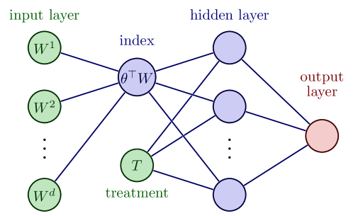
Figure 7. Neural network architecture for single-index model.

The neural network architecture is illustrated in Figure 7. The network was optimized using MSE loss and the ADAM optimizer with lr=1e-3 and n_iter=1200 in the simulation experiment. For the NHANES application the settings were similar, but with BCELoss and n_iter=3000. We discovered that the optimization procedure could get stuck in a local minimum with significantly lower training score. To avoid getting stuck in a such a ‘bad local minimum’, it was possible to refit the network with random initialization several times and pick the model with highest training score. The frequency of bad local minimums is roughly $15\%$, with variation between each setting. Thus, refitting the network, say 5 times, is enough to avoid a bad minimum $>99,99\%$ of the time. To save the computational cost of refitting many times for each simulation, we initialized the first layer with an initial value $\theta_{init}=\beta+\mathrm{Unif}(-0.1,0.1)^{\otimes d}$. The Logistic regression for the propensity score was fitted without $\ell_{2}$-penalty and optimized using the lbfgs optimizer. The propensity score was clipped to the interval $(0.01,0.99)$ for all estimators of the adjusted mean.

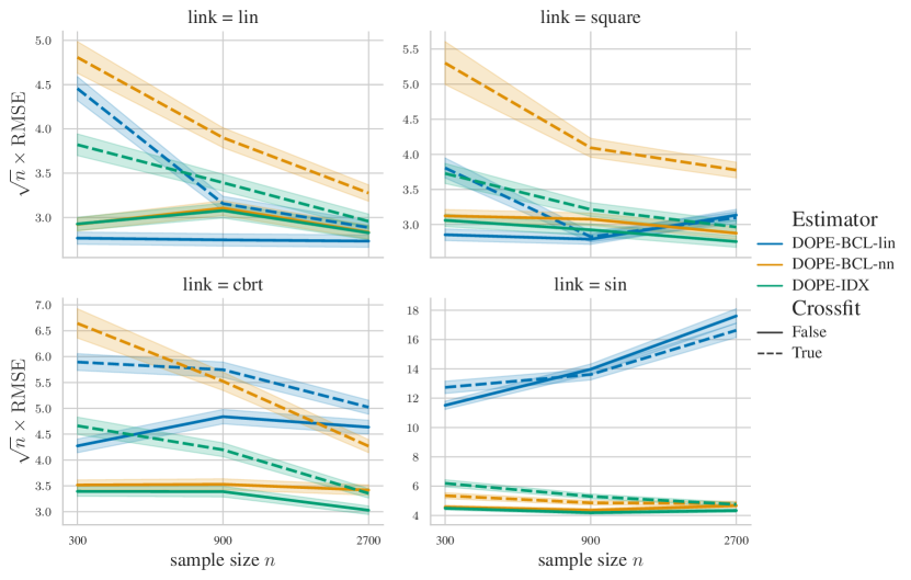
Figure 8. Comparison of DOPE estimators with and without sample splitting.

Figure 8 shows the cross-fitted DOPE estimators versus their full sample counterparts in the simulation setup of Section 5.1. We observe that cross-fitting generally seems to decrease performance for small sample sizes, but the discrepancy diminishes for larger sample sizes.

Estimator	Estimate	BS se	BS CI
Regr. (NN)	0.020	0.008	(0.002, 0.035)
Regr. (Logistic)	0.027	0.009	(0.012, 0.048)
DOPE-BCL (Logistic)	0.024	0.010	(0.004, 0.040)
Naive contrast	0.388	0.010	(0.369, 0.407)
DOPE-BCL (NN)	0.018	0.010	(-0.003, 0.036)
DOPE-IDX (NN)	0.023	0.012	(-0.001, 0.047)
AIPW (NN)	0.017	0.016	(-0.017, 0.046)
AIPW (Logistic)	0.022	0.016	(-0.012, 0.051)
IPW (Logistic)	-0.047	0.027	(-0.119, -0.01)

Table 2. Treatment effect estimates for NHANES dataset, where covariates with more than 50% missing values have been removed.

Table 2 corresponds to Table 1 in the main manuscript, but where covariates with more than $50\%$ missing data have been removed rather than imputed. Except for the naive contrast (which has dropped two rows) the ordering according to bootstrap variance is the same.

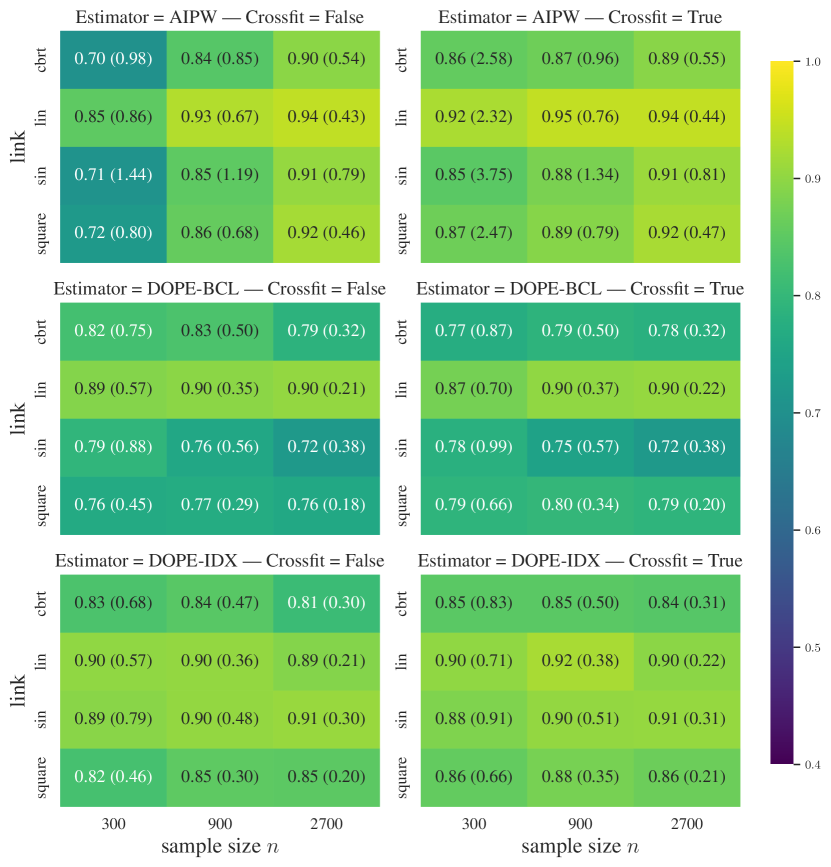
Figure 9. Coverage of asymptotic confidence intervals of the adjusted mean $\chi_{1}$, aggregated over $d\in\{4,12,36\}$ and with the true $\beta$ given in (5.1.1). The numbers in the parentheses denote the corresponding average width of the confidence interval.

Figure 9 shows the same coverage values as Figure 5, but also includes the average lengths of the confidence intervals in the parentheses. We note that the lengths of the confidence intervals for the DOPE estimators are much smaller than those of the AIPW estimator.

Appendix C Extension to cross-fitting

1 input: observations $(T_{i},\mathbf{W}_{i},Y_{i})_{i\in[n]}$, partition $[n]=J_{1}\cup\cdots\cup J_{K}$;

2 options: integer $1\leq m\leq K-2$ and options for Algorithm 1;

3 for $k=1,\ldots,K$ do

4       Set $\mathcal{I}_{3}=J_{k}$, $\mathcal{I}_{1}=\bigcup_{l=k+1}^{k+m}J_{l}$ and $\mathcal{I}_{2}=[n]\setminus(\mathcal{I}_{1}\cup\mathcal{I}_{3})$;

5      

6      Compute $\widehat{\chi}_{t,k}^{\mathrm{dope}}$ as the output of Algorithm 1;

7      

8      Compute variance estimate $\widehat{\mathcal{V}}_{t,k}$ given as in (17);

9      

10 end for

return $\widehat{\chi}_{t}^{\mathsf{x}}\coloneq\frac{1}{K}\sum_{k=1}^{K}\widehat{\chi}_{t,k}^{\mathrm{dope}}$ and $\widehat{\mathcal{V}}_{t}^{\mathsf{x}}\coloneq\frac{1}{K}\sum_{k=1}^{K}\widehat{\mathcal{V}}_{t,k}$

Algorithm 2 Cross-fitted DOPE

A cross-fitting procedure for the DOPE is described in Algorithm 2, which computes both a cross-fitted version of the DOPE and its variance estimator. Here the indices of the folds are understood to cycle modulo $K$ such that $J_{K+1}=J_{1}$ and so forth. This version of cross-fitting with three index sets has also been referred to as ‘double cross-fitting’ by Zivich & Breskin (2021).

We note that the ‘standard arguments’ for establishing convergence of the cross-fitted estimator cannot be applied directly to our case. This is because, for each fold $k\in[K]$, the corresponding oracle terms $U_{\hat{\theta}_{k}}^{(n)}$ do not only involve the data indexed by $\mathcal{I}_{3}^{k}$, but also depend on $\hat{\theta}_{k}$ which is estimated from data indexed by $\mathcal{I}_{1}^{k}$. Hence the oracle terms are not independent. However, we believe that this dependency should be negligible, and perhaps the convergence can be established under a more refined theoretical analysis.

References

• (1)
• Baldé et al. (2023) Baldé, I., Yang, Y. A. & Lefebvre, G. (2023), ‘Reader reaction to “Outcome-adaptive lasso: Variable selection for causal inference” by Shortreed and Ertefaie (2017)’, Biometrics 79(1), 514–520.
• Benkeser et al. (2020) Benkeser, D., Cai, W. & Laan, M. (2020), ‘A nonparametric super-efficient estimator of the average treatment effect’, Statistical Science 35, 484–495.
• Benkeser & van der Laan (2016) Benkeser, D. & van der Laan, M. (2016), The highly adaptive lasso estimator, in ‘2016 IEEE international conference on data science and advanced analytics (DSAA)’, IEEE, pp. 689–696.
• Billingsley (2017) Billingsley, P. (2017), Probability and measure, John Wiley & Sons.
• Bojer & Meldgaard (2021) Bojer, C. S. & Meldgaard, J. P. (2021), ‘Kaggle forecasting competitions: An overlooked learning opportunity’, International Journal of Forecasting 37(2), 587–603.
• Chernozhukov et al. (2018) Chernozhukov, V., Chetverikov, D., Demirer, M., Duflo, E., Hansen, C., Newey, W. & Robins, J. (2018), ‘Double/debiased machine learning for treatment and structural parameters’, The Econometrics Journal 21(1), C1–C68.
• Chickering et al. (2004) Chickering, M., Heckerman, D. & Meek, C. (2004), ‘Large-sample learning of bayesian networks is NP-hard’, Journal of Machine Learning Research 5, 1287–1330.
• Christgau et al. (2023) Christgau, A. M., Petersen, L. & Hansen, N. R. (2023), ‘Nonparametric conditional local independence testing’, The Annals of Statistics 51(5), 2116–2144.
• Cox et al. (1997) Cox, C. S., Feldman, J. J., Golden, C. D., Lane, M. A., Madans, J. H., Mussolino, M. E. & Rothwell, S. T. (1997), ‘Plan and operation of the NHANES I epidemiologic follow-up study, 1992’, Vital and health statistics. .
• Delecroix et al. (2003) Delecroix, M., Härdle, W. & Hristache, M. (2003), ‘Efficient estimation in conditional single-index regression’, Journal of Multivariate Analysis 86(2), 213–226.
• Devlin et al. (2018) Devlin, J., Chang, M.-W., Lee, K. & Toutanova, K. (2018), ‘BERT: Pre-training of deep bidirectional transformers for language understanding’, arXiv:1810.04805 .
• Émery & Schachermayer (2001) Émery, M. & Schachermayer, W. (2001), On Vershik’s standardness criterion and Tsirelson’s notion of cosiness, in ‘Séminaire de Probabilités XXXV’, Springer, pp. 265–305.
• Forré & Mooij (2023) Forré, P. & Mooij, J. M. (2023), ‘A mathematical introduction to causality’.
• Franklin et al. (1999) Franklin, S. S., Khan, S. A., Wong, N. D., Larson, M. G. & Levy, D. (1999), ‘Is pulse pressure useful in predicting risk for coronary heart disease? The Framingham heart study’, Circulation 100(4), 354–360.
• Gnecco et al. (2023) Gnecco, N., Peters, J., Engelke, S. & Pfister, N. (2023), ‘Boosted control functions’, arXiv:2310.05805 .
• Greenewald et al. (2021) Greenewald, K., Shanmugam, K. & Katz, D. (2021), High-dimensional feature selection for sample efficient treatment effect estimation, in ‘International Conference on Artificial Intelligence and Statistics’, PMLR, pp. 2224–2232.
• Guo et al. (2022) Guo, F. R., Lundborg, A. R. & Zhao, Q. (2022), ‘Confounder selection: Objectives and approaches’, arXiv:2208.13871 .
• Hahn (1998) Hahn, J. (1998), ‘On the role of the propensity score in efficient semiparametric estimation of average treatment effects’, Econometrica pp. 315–331.
• Hansen (2008) Hansen, B. B. (2008), ‘The prognostic analogue of the propensity score’, Biometrika 95(2), 481–488.
• Henckel et al. (2022) Henckel, L., Perković, E. & Maathuis, M. H. (2022), ‘Graphical criteria for efficient total effect estimation via adjustment in causal linear models’, Journal of the Royal Statistical Society Series B: Statistical Methodology 84(2), 579–599.
• Homan et al. (2024) Homan, T., Bordes, S. & Cichowski, E. (2024), ‘Physiology, pulse pressure’. [Updated 2023 Jul 10].
• Ichimura (1993) Ichimura, H. (1993), ‘Semiparametric least squares (SLS) and weighted SLS estimation of single-index models’, Journal of Econometrics 58(1-2), 71–120.
• Ju et al. (2020) Ju, C., Benkeser, D. & van der Laan, M. J. (2020), ‘Robust inference on the average treatment effect using the outcome highly adaptive lasso’, Biometrics 76(1), 109–118.
• Ju et al. (2019) Ju, C., Gruber, S., Lendle, S. D., Chambaz, A., Franklin, J. M., Wyss, R., Schneeweiss, S. & van der Laan, M. J. (2019), ‘Scalable collaborative targeted learning for high-dimensional data’, Statistical methods in medical research 28(2), 532–554.
• Kallenberg (2021) Kallenberg, O. (2021), Foundations of Modern Probability, 3 edn, Springer International Publishing.
• Kolmogoroff (1933) Kolmogoroff, A. (1933), Grundbegriffe der Wahrscheinlichkeitsrechnung, Ergebnisse der Mathematik und Ihrer Grenzgebiete. 1. Folge, 1 edn, Springer Berlin, Heidelberg.
• Lundberg et al. (2020) Lundberg, S. M., Erion, G., Chen, H., DeGrave, A., Prutkin, J. M., Nair, B., Katz, R., Himmelfarb, J., Bansal, N. & Lee, S.-I. (2020), ‘From local explanations to global understanding with explainable AI for trees’, Nature machine intelligence 2(1), 56–67.
• Lundborg & Pfister (2023) Lundborg, A. R. & Pfister, N. (2023), ‘Perturbation-based analysis of compositional data’, arXiv:2311.18501 .
• Parkinson et al. (2023) Parkinson, S., Ongie, G. & Willett, R. (2023), ‘Linear neural network layers promote learning single-and multiple-index models’, arXiv:2305.15598 .
• Paszke et al. (2019) Paszke, A., Gross, S., Massa, F., Lerer, A., Bradbury, J., Chanan, G., Killeen, T., Lin, Z., Gimelshein, N., Antiga, L., Desmaison, A., Kopf, A., Yang, E., DeVito, Z., Raison, M., Tejani, A., Chilamkurthy, S., Steiner, B., Fang, L., Bai, J. & Chintala, S. (2019), Pytorch: An imperative style, high-performance deep learning library, in ‘Advances in Neural Information Processing Systems 32’, Curran Associates, Inc., pp. 8024–8035.
• Pearl (2009) Pearl, J. (2009), Causality, Cambridge University Press.
• Pedregosa et al. (2011) Pedregosa, F., Varoquaux, G., Gramfort, A., Michel, V., Thirion, B., Grisel, O., Blondel, M., Prettenhofer, P., Weiss, R., Dubourg, V., Vanderplas, J., Passos, A., Cournapeau, D., Brucher, M., Perrot, M. & Duchesnay, E. (2011), ‘Scikit-learn: Machine learning in Python’, Journal of Machine Learning Research 12, 2825–2830.
• Perković et al. (2018) Perković, E., Textor, J., Kalisch, M. & Maathuis, M. H. (2018), ‘Complete graphical characterization and construction of adjustment sets in markov equivalence classes of ancestral graphs’, Journal of Machine Learning Research 18(220), 1–62.
• Peters et al. (2017) Peters, J., Janzing, D. & Schölkopf, B. (2017), Elements of causal inference: foundations and learning algorithms, The MIT Press.
• Powell et al. (1989) Powell, J. L., Stock, J. H. & Stoker, T. M. (1989), ‘Semiparametric estimation of index coefficients’, Econometrica: Journal of the Econometric Society pp. 1403–1430.
• Robins & Rotnitzky (1995) Robins, J. M. & Rotnitzky, A. (1995), ‘Semiparametric efficiency in multivariate regression models with missing data’, Journal of the American Statistical Association 90(429), 122–129.
• Robins et al. (1994) Robins, J. M., Rotnitzky, A. & Zhao, L. P. (1994), ‘Estimation of regression coefficients when some regressors are not always observed’, Journal of the American statistical Association 89(427), 846–866.
• Rosenbaum & Rubin (1983) Rosenbaum, P. R. & Rubin, D. B. (1983), ‘The central role of the propensity score in observational studies for causal effects’, Biometrika 70(1), 41–55.
• Rotnitzky & Smucler (2020) Rotnitzky, A. & Smucler, E. (2020), ‘Efficient adjustment sets for population average causal treatment effect estimation in graphical models.’, Journal of Machine Learning Research 21(188), 1–86.
• Schölkopf et al. (2021) Schölkopf, B., Locatello, F., Bauer, S., Ke, N. R., Kalchbrenner, N., Goyal, A. & Bengio, Y. (2021), ‘Toward causal representation learning’, Proceedings of the IEEE 109(5), 612–634.
• Shah & Peters (2020) Shah, R. D. & Peters, J. (2020), ‘The hardness of conditional independence testing and the generalised covariance measure’, The Annals of Statistics 48(3), 1514 – 1538.
• Shi et al. (2019) Shi, C., Blei, D. & Veitch, V. (2019), ‘Adapting neural networks for the estimation of treatment effects’, Advances in neural information processing systems 32.
• Shortreed & Ertefaie (2017) Shortreed, S. M. & Ertefaie, A. (2017), ‘Outcome-adaptive lasso: variable selection for causal inference’, Biometrics 73(4), 1111–1122.
• Smucler et al. (2019) Smucler, E., Rotnitzky, A. & Robins, J. M. (2019), ‘A unifying approach for doubly-robust l1-regularized estimation of causal contrasts’, arXiv:1904.03737 .
• Uhler et al. (2013) Uhler, C., Raskutti, G., Bühlmann, P. & Yu, B. (2013), ‘Geometry of the faithfulness assumption in causal inference’, The Annals of Statistics pp. 436–463.
• van der Laan & Gruber (2010) van der Laan, M. J. & Gruber, S. (2010), ‘Collaborative double robust targeted maximum likelihood estimation’, The international journal of biostatistics 6(1).
• van der Laan & Rose (2011) van der Laan, M. J. & Rose, S. (2011), Targeted learning: causal inference for observational and experimental data, Vol. 4, Springer.
• van der Vaart (2000) van der Vaart, A. W. (2000), Asymptotic statistics, Vol. 3, Cambridge university press.
• Van Rossum et al. (1995) Van Rossum, G., Drake, F. L. et al. (1995), Python reference manual, Vol. 111, Centrum voor Wiskunde en Informatica Amsterdam.
• Veitch et al. (2020) Veitch, V., Sridhar, D. & Blei, D. (2020), Adapting text embeddings for causal inference, in ‘Conference on Uncertainty in Artificial Intelligence’, PMLR, pp. 919–928.
• Zivich & Breskin (2021) Zivich, P. N. & Breskin, A. (2021), ‘Machine learning for causal inference: on the use of cross-fit estimators’, Epidemiology (Cambridge, Mass.) 32(3), 393.