How Temporal Unrolling Supports Neural Physics Simulators

Abstract

Unrolling training trajectories over time strongly influences the inference accuracy of neural network-augmented physics simulators. We analyze these effects by studying three variants of training neural networks on discrete ground truth trajectories. In addition to commonly used one-step setups and fully differentiable unrolling, we include a third, less widely used variant: unrolling without temporal gradients. Comparing networks trained with these three modalities makes it possible to disentangle the two dominant effects of unrolling, training distribution shift and long-term gradients. We present a detailed study across physical systems, network sizes, network architectures, training setups, and test scenarios. It provides an empirical basis for our main findings: A non-differentiable but unrolled training setup supported by a numerical solver can yield 4.5-fold improvements over a fully differentiable prediction setup that does not utilize this solver. We also quantify a difference in the accuracy of models trained in a fully differentiable setup compared to their non-differentiable counterparts. While differentiable setups perform best, the accuracy of unrolling without temporal gradients comes comparatively close. Furthermore, we empirically show that these behaviors are invariant to changes in the underlying physical system, the network architecture and size, and the numerical scheme. These results motivate integrating non-differentiable numerical simulators into training setups even if full differentiability is unavailable. We also observe that the convergence rate of common neural architectures is low compared to numerical algorithms. This encourages the use of hybrid approaches combining neural and numerical algorithms to utilize the benefits of both.

1 Introduction

Our understanding of physical systems relies on capturing their dynamics in mathematical models, often representing them with a partial differential equation (PDE). Forecasting the behavior with these models thus involves the notoriously costly and difficult task of solving the PDE. By aiming to increase simulator efficiencies, machine learning was successfully deployed to augment traditional numerical methods for solving these equations. Common areas of research are network architectures [51, 33, 19, 57], reduced order representations [38, 65, 16, 10, 68], and training methods [56, 52, 39, 7]. Previous studies were further motivated by performance and accuracy boosts offered by these methods, especially on GPU architectures. Especially computational fluid dynamics represents an application of machine learning augmented solvers [4, 13]. Potential applications in turbulence include closure modeling in Reynolds-averaged Navier-Stokes modeling [35, 71, 72] as well as closure models for large eddy simulation [43, 2, 37, 52, 58].

Out of all physical systems of interest in simulations, those exhibiting transient dynamics are particularly challenging to model. Solutions to these systems are typically based on a time-discrete evolution of the underlying dynamics. Consequently, the simulator of such dynamics is subject to many auto-regressive invocations. Designing simulators that achieve stability and accuracy over long auto-regressive horizons can be challenging in numerical and neural settings. However, unlike numerical approaches, where unstable components such as dispersion errors are well studied and effective stabilizing approaches exist, little is known about the origin of instabilities and mitigating strategies for neural networks. As an interesting development, a stability analysis of echo-state networks was presented recently [40], allowing deeper insights into the behavior of recurrent networks. Nevertheless, stabilizing autoregressive neural simulators remains particularly difficult. One promising strategy is unrolling discrete trajectories at training time, improving long-term stability in different settings [56, 28, 52]. It is now a common approach when training neural networks that predict PDE trajectories on their own, or support numerical solvers in doing so. However, we still lack a systemic understanding of unrolling and its effects on network training.

Within this paper, we explore unrolling from a dynamical systems perspective. A first fundamental insight is that no machine-learned approximation identically fits the underlying target. For physics simulators, this means that the dynamics of the learned system will always differ from the target dynamics. As such, the attractors for the target and the learned system do not coincide entirely. Unrolling can be seen as an exploration of the machine-learned dynamics’ attractor at training time. In contrast to training without unrolling, this approach thus allows sampling from a different distribution in the solution space. An unrolled training procedure samples from the learned dynamics and exposes (more of) the inference attractor at training time. As such, this difference between training and inference, commonly known as data shift in the machine learning community, is reduced. For longer horizons, more of the learned dynamics’ attractor is exposed, stabilizing the neural simulator.

In principle, this would motivate ever longer horizons, as illustrated in Figure 1. However, obtaining useful gradients through unrolled dynamical systems limits this horizon in practice [11]. The differentiability of numerical solvers is crucial to backpropagate through solver-network chains. However, if the learned system exhibits chaotic behavior, backpropagating long unrolled chains can lead to instabilities in the gradient calculation itself [42]. Due to the strong non-linearities of deep-learning architectures, the auto-regressive dynamics of the learned simulator can show chaotic behavior in early training stages, regardless of the properties of the target system. A limitation to the effective unrolled horizon in fully differentiable setups was thus observed in previous studies [56, 37].

A central and rarely used variant employs unrolling without backpropagating gradients through the simulator. We study this training variant in detail because of its high practical relevance, as it can be realized by integrating existing, non-differentiable solvers into a deep learning framework. The forward pass of a non-differentiable unrolling setup is identical to the fully differentiable setup and thus features the same attractor-fitting property. In the backward pass, gradients are set to zero whenever they need to be propagated through a numerical solver. This effectively truncates the backpropagation, and avoids long gradient propagation chains. While cutting gradients potentially has a stabilizing effect, we find that it also limits the effective unrolling horizon, albeit for different reasons: the computed gradient approximations diverge from the true gradient as the unrolling horizon increases, making the learning process less reliable. Figure 1 illustrates these gradient inaccuracies for both training modalities. To the best of our knowledge, extensive studies of non-differentiable unrolled training do not yet exist. This is despite its high relevance to the scientific computing community as an approachable variant integrating numerical solvers in network training.

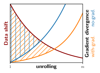
Figure 1: Illustration of data shift and gradient divergence over unrolling; gradients of non-differentiable unrolling diverge from the true gradient landscape (blue), gradients of differentiable simulators are prone to explosions over long horizons (orange); shaded areas mark potential benefits over one-step learning; full gradient calculation performs best.

We analyze these two unrolling variants using standardized solver and network architectures, while contrasting them with one-step training. This allows disentangling the effects of training data shift introduced by forward unrolling and accurate long-term gradients calculated by backpropagation. We test our findings on various physical systems with multiple network architectures, including convolutional and graph networks. Five recommendations for unrolled neural simulators training are derived from our results:

(I) Non-differentiable unrolling as an alternative

The mitigating effects on data shift introduced by unrolling can boost model performance. An unrolled but non-differentiable chain can increase performance by 23% on average. In addition, non-differentiable neural hybrid simulators do not require a new implementation of existing numerical solvers and thus represent an attractive alternative for fields with large traditional code bases. When no differentiable implementations are available, previous work typically resorts to pure prediction models. Instead, our results strongly encourage interfacing non-differentiable numerical implementations with machine learning, as doing so yields up to 4.5-fold accuracy improvements over prediction setups for identical network architectures and sizes.

(II) Differentiable unrolling delivers the best accuracy

When other hyperparameters are fixed, a differentiable unrolling strategy consistently outperforms other setups. At the cost of increased software engineering efforts, differentiable unrolling outperforms its one-step counterpart by 38% on average. Long-term gradients prove to be especially important for hybrid setups where neural networks correct numerical solvers.

(III) Hybrid approaches yield improved scaling:

Our study across network sizes finds them predominant regarding accuracy on inter- and extrapolative tests. However, we observe suboptimal convergence of the inference error when increasing the parameter count. These convergence rates compare poorly to the ones usually observed for numerical solvers. Most neural PDE simulators directly compete with numerical solvers. Thus, scaling to larger problems is critical for neural simulators. Unrolling can effectively train hybrid simulators even when integrated with a non-differentiable solver. These combine the benefits of neural networks with the scaling properties of numerical solvers.

(IV) Low-dimensional problems match

Our results translate between physical systems. Provided the systems are from a similar domain, i.e. we primarily consider turbulent chaotic systems, high-level training behaviors translate between physical systems. This validates the approach common in other papers, where broad studies were conducted on low-dimensional systems and only tested on the high-dimensional target.

(V) Curriculums are necessary

The training of unrolled setups is non-trivial and sensitive to hyperparameters. Reliable training setups utilize a curriculum where the unrolled number of steps slowly increases. The learning rate needs to be adjusted to keep the amplitude of the gradient feedback at a stable level. Our work takes a task- and architecture-agnostic stance. Combined with the large scale of evaluations across more than three thousand models, this allows for extracting general trends and the aforementioned set of recommendations. Source code and training data will be made available upon acceptance.

2 Related work

Data-driven PDE solvers:

Machine learning based simulators aim to address the limitations of classical PDE solvers in challenging scenarios with complex dynamics [18, 60, 9]. While physics-informed networks have gained popularity in continous PDE modeling [48, 13], many learned approaches work in a purely data-driven manner on discrete trajectories. Several of these use advanced network architectures to model the time-evolution of the PDE, such as graph networks [46, 51], problem-tailored architectures [61, 53], bayesian networks [70], generative adverserial networks [67], transformer models [22, 20, 32], or lately diffusion models [34, 36, 29]. Variations of these approaches compute the evolution in an encoded latent space [65, 19, 20, 10, 68, 59].

Unrolled training:

Fitting an unrolled ground truth trajectory is frequently used for training autoregressive methods. This can be done with unrolled architectures that solely rely on networks [19], or for networks that correct solvers [56, 28, 39, 41]. For the latter, differentiable or adjoint solvers allow backpropagation of gradients through the entire chain [25, 52, 24]. The studies building on these solvers report improved network performance for longer optimization horizons. However, differentiability is rarely satisfied in existing code bases. A resulting open question is how much the numerical solver’s differentiability assists in training accurate networks. As the introduction mentions, two properties of differentiable unrolling affect the training procedure. The data shift moves the observed training data closer toward realistic inference scenarios [66, 62]. For instance, [7, 47] proposed variations of classic truncation [55], and reported a positive effect on the network performance, where ”warm-up” steps without contribution to the learning signal stabilize the trained networks. The differentiability of the numerical solver introduces the second property, which allows the propagation of gradients through time evolutions. The resulting loss landscape better approximates temporal extrapolation, which benefits model performance [56, 52, 28]. Recently, possible downsides of differentiable unrolling concerning gradient stability were investigated. While a vanishing/exploding effect is well known for recurrent networks, it is only sparsely studied for hybrid approaches. It was found that the stability of the backpropagation gradients aligns with the Lyapunov time of the physical system for recurrent prediction networks [42]. As a potential remedy, it was proposed to cut the backpropagation chain into individual sequences [37].

Benchmarks and datasets:

Several benchmarks and datasets have been published to increase comparability and promote standardization of machine-learned PDE simulators, especially in fluid mechanics. A dataset of measured real-world smoke clouds can be found in [14]. A high-fidelty Reynolds-averaged Navier-Stokes dataset is provided in [6]. Furthermore, more specialized datasets like [69] focus on fluid manipulation and robotics. A dataset of large-scale $2$D fluid flows on non-uniform meshes and a benchmark for transformer models are also available [27]. As we focus on tasks that correct solvers, we evaluate our models on frameworks with differentiable solvers [24, 56].

3 Unrolling PDE Evolutions

Unrolling is a common strategy for learning time sequences. A first important distinction is whether the task at hand is a prediction or a correction task. Additionally, we formally introduce the differences between non-differentiable and differentiable unrolling in gradient calculation. These are then used to derive an intuition about the gradient effects of unrolling.

3.1 Evolving partial differential equations with neural networks

Let us consider the general formulation of a PDE in the form of

$$\frac{\partial\mathbf{u}}{\partial t}=\mathcal{F}(\mathbf{u},\nabla\mathbf{u},\nabla^{2}\mathbf{u},\dots),$$ (1)

with $\mathbf{u}$ representing the field variables of the physical system. The dynamics of $\mathcal{F}$ have an attractor $A_{\mathcal{F}}$ representing a subspace of the solution space. A state contained in $A_{\mathcal{F}}$ will always evolve to other states on $A_{\mathcal{F}}$, while states in the neighborhood of $A_{\mathcal{F}}$ converge to this attractor. We study Neural Simulator architectures that use neural networks for evolving discretized forms of PDE s. They are autoregressively applied to generate trajectories of discrete $\mathbf{u}^{t}$. Prediction setups fully rely on a neural network to calculate the next timestep as $\mathbf{u}^{t+1}=f_{\theta}(\mathbf{u}^{t})$, where $\theta$ represents the parameters of the network function. In a prediction configuration, the network fully replaces a numerical solver with the goal of improving its accuracy and performance. Similarly, correction setups are also concerned with time-evolving a discretized PDE but additionally include a physical prior $\mathcal{S}$ that approximates the solution. The network then corrects this approximation such that $\mathbf{u}^{t+1}=f_{\theta}(\mathcal{S}(\mathbf{u}^{t}))$. These architectures represent a hybrid between numerical and neural architectures, potentially combining the advantages of both domains. Possible applications include, turbulence modeling in RANS or LES, as well as dynamical system control setups.

Crucially, inputs and outputs of the networks live in the space of the solution vector field, both for predictive and corrective setups. Thus, we use different instances of the same architecture in both setups. We use the same notation $f_{\theta}$ for both applications to stress this property.

3.2 Unrolling dynamical systems at training time

Unrolling describes the process of auto-regressively evolving the learned system in a training iteration. It can be formalized as

$$\mathbf{u}^{t+s}=g_{\theta}^{s}(\mathbf{u}^{t}),$$ (2)

where $g^{s}$ represents the recurrent application of $s$ steps of either correction, for which $g_{\theta}(\mathbf{u})=f_{\theta}(\mathcal{S}(\mathbf{u}))$, or prediction, where $g_{\theta}(\mathbf{u})=f_{\theta}(\mathbf{u})$. Similarly to the target dynamics, the learned system also has an attractor $A_{g_{\theta}}$ defining its solution space. When unrolling a learning trajectory, multiple frames $[\mathbf{u}^{t+1},\mathbf{u}^{t+2},\dots,\mathbf{u}^{t+m}$] are generated, where $m$ denotes the number of unrolled time steps. A simple one-step training is obtained by setting $m=1$. The objective of the neural network is to fit the PDE dynamics in equation 1. The network models are trained to represent the underlying PDE by fitting a dataset of ground truth trajectories $\tilde{U}=[\mathbf{\tilde{u}}^{0}\dots\mathbf{\tilde{u}}^{N}]$. This dataset contains samples from the target attractor $A_{\mathcal{F}}$, which represents a subset of the phase space of $\mathbf{\tilde{u}}$ restricted to physical solutions. Nevertheless, due to imperfections in the learned solution, the learned dynamics (2) will differ from the ground truth at training and inference time. Thus, the learned attractor $A_{g_{\theta}}\neq A_{\mathcal{F}}$.

Crucially, training without unrolling does not guarantee that the states $\mathbf{u}$ observed during training sufficiently represent $A_{g_{\theta}}$. In other words,

$$\forall\mathbf{\tilde{u}}^{i}\in A_{\mathcal{F}},A_{g_{\theta}}:\lim_{N\rightarrow\infty}\{g_{\theta}(\mathbf{\tilde{u}}^{0}),g_{\theta}(\mathbf{\tilde{u}}^{1}),...,g_{\theta}(\mathbf{\tilde{u}}^{N})\}\neq A_{g_{\theta}}.$$ (3)

This means that we are not guaranteed to explore the attractor of the learned system $A_{g_{\theta}}$ when only observing states based on one discrete evolution of $g_{\theta}$, regardless of the dataset size $N$. A common data-augmentation approach is to perturb the ground truth states in $\tilde{U}$ with noise, in the hope that the perturbed states fit $A_{g_{\theta}}$ more closely [51]. While this approach was reported to be successful, it still does not provide a guarantee that the observed states are physical under $g_{\theta}$.

Let us now suppose we unroll $m$ steps with $g_{\theta}^{s}(\mathbf{\tilde{u}})$. Based on the definition of the attractor $A_{g_{\theta}}$ we can state that

$$\lim_{m\rightarrow\infty}\{g_{\theta}^{0}(\mathbf{\tilde{u}}^{i}),g_{\theta}^{1}(\mathbf{\tilde{u}}^{i}),...,g_{\theta}^{m}(\mathbf{\tilde{u}}^{i})\}=A_{g_{\theta}},$$ (4)

for any $\mathbf{\tilde{u}}^{i}$ in the vicinity of $A_{g_{\theta}}$. While the horizon $m$ is practically never chosen long enough to expose $A_{g_{\theta}}$ with a single initial condition, a sufficiently large dataset ensures that $A_{g_{\theta}}$ is approached from multiple angles. In contrast to training wihtout unrolling, enabling it thus exposes the inference attractor $A_{g_{\theta}}$ at training time for sufficiently large datasets and horizons $m$. Precisely the difference between the observed training set (sampled from $A_{\mathcal{F}}$) and the inference attractor $A_{g_{\theta}}$ is commonly known as data shift in machine learning. The dark red curve in Figure 1 shows how this data shift is thus reduced by choosing larger $m$.

3.3 Training neural networks to solve PDEs:

The general training procedure is given as

$$\theta^{*}=\mathrm{arg}\min_{\theta}\bigg{[}\sum_{i=1}^{N-m}\sum_{s={1}}^{m}\mathcal{L}_{2}\big{(}\tilde{\mathbf{u}}^{i+s\tau},g_{\theta}^{s}(\mathbf{u}^{i})\big{)}\bigg{]},$$ (5)

where $\tau$ accounts for the relative timestep between ground truth and predicted trajectories. For one learning iteration, a loss value is accumulated over an unrolled trajectory. We can write this total loss over the unrolled trajectory as

$$\mathcal{L}=\sum_{i=1}^{s}\mathcal{L}_{2}(\tilde{\mathbf{u}}^{i+\tau s},g^{s}_{\theta}(\mathbf{u}^{i}))=\sum_{i=1}^{s}\mathcal{L}^{s},$$ (6)

where $\mathcal{L}^{s}$ represents the loss evaluated after a step. The simplest realization of the training procedure (5) utilizes the forward process with $m=1$, i.e. no unrolling. We refer to this variant without unrolling as one-step (ONE) in the following. This approach is common practice in literature and the resulting training procedure is easily realized with pre-computed data. In contrast, the full backpropagation through an unrolled chain with $m>1$ requires a differentiable solver $\mathcal{S}$ for the correction setup. The differentiable setup can calculate the full optimization gradients by propagating gradients through a simulation step. The gradients are thus evaluated as

$$\frac{\partial\mathcal{L}_{\mathrm{WIG}}^{s}}{\partial\theta}=\sum_{B=1}^{s}\bigg{[}\frac{\partial\mathcal{L}^{s}}{\partial g_{\theta}^{s}}\bigg{(}\prod_{b=1}^{s-B}\frac{\partial g_{\theta}^{s-b}}{\partial g_{\theta}^{s-b-1}}\bigg{)}\frac{\partial g_{\theta}^{B}}{\partial\theta}\bigg{]}.$$ (7)

We refer to this fully differentiable setup as with-gradient (WIG). The gradient flow through a simulator step $g$ is caluclated as $\frac{\partial g_{\theta}^{s+1}}{\partial g_{\theta}^{s}}=\frac{\partial f_{\theta}^{s}}{\partial\mathcal{S}^{s}}\frac{\partial\mathcal{S}^{s}}{\partial g_{\theta}^{s}}$ for correction setups and as $\frac{\partial g_{\theta}^{s+1}}{\partial g_{\theta}^{s}}=\frac{\partial f_{\theta}^{s}}{\partial g_{\theta}^{s}}$ for prediction. To test the effect of differentiability, we introduce a second strategy for propagating the gradients $\frac{\partial\mathcal{L}^{s}}{\partial\theta}$. If no differentiable solver is available, optimization gradients can only propagate to the network application, not through the solver. The gradients are thus evaluated as

$$\frac{\partial\mathcal{L}_{\mathrm{NOG}}^{s}}{\partial\theta}=\frac{\partial\mathcal{L}^{s}}{\partial g_{\theta}^{s}}\frac{\partial g_{\theta}^{s}}{\partial\theta}.$$ (8)

This setup is referred to as no-gradient (NOG). Here, $\frac{\partial g_{\theta}^{s+1}}{\partial g_{\theta}^{s}}:=0$ holds for correction and prediction setups. Thus, a simulator step in the NOG setup is not differentiable and yields no gradients. Most existing code bases in engineering and science are not fully differentiable. Consequentially, this NOG setup is particularly relevant, as it could be implemented using existing traditional numerical solvers.

Table 1: Calculated gradients with unrolled step $s$; for correction: $\frac{\partial g^{s+1}}{\partial g^{s}}=\frac{\partial f_{\theta}^{s}}{\partial\mathcal{S}^{s}}\frac{\partial\mathcal{S}^{s}}{\partial g^{s}}$; for prediction: $\frac{\partial g^{s+1}}{\partial g^{s}}=\frac{\partial f_{\theta}^{s}}{\partial g^{s}}$

	$\mathcal{L}$	$\partial\mathcal{L}/\partial\theta$	Requires diff. $\mathcal{S}$	Realization
ONE	$\mathcal{L}_{2}^{1}$	$\dfrac{\partial\mathcal{L}_{2}^{1}}{\partial f^{1}_{\theta}}\dfrac{\partial f^{1}_{\theta}}{\partial\theta}$	no	precompute
NOG	$\sum\limits_{s}\mathcal{L}_{2}^{s}$	$\sum\limits_{s}\dfrac{\partial\mathcal{L}_{2}^{s}}{\partial f^{s}_{\theta}}\dfrac{\partial f^{s}_{\theta}}{\partial\theta}$	no	interface
WIG	$\sum\limits_{s}\mathcal{L}_{2}^{s}$	$\sum\limits_{s}\sum\limits_{B=1}^{s}\dfrac{\partial\mathcal{L}^{s}_{2}}{\partial{g}^{s}}\dfrac{\partial g^{s}}{\partial g^{B}}\dfrac{\partial g^{B}}{\partial\theta}$	yes	re-implement

Figure 2 contains a visualization including the backpropagation flow through an unrolled chain. The gradient calculations for our three setups are further denoted in table 1. Further detail of the gradient calculations in correction and prediction setups is found in A.

3.4 Gradient behavior in unrolled systems

As WIG unrolling provides the true gradient, we can thus derive the gradient inaccuracy of the NOG setup as

$$\frac{\partial\mathcal{L}_{\mathrm{WIG}}}{\partial\theta}-\frac{\partial\mathcal{L}_{\mathrm{NOG}}}{\partial\theta}=\sum_{s=1}^{m}\sum_{B=1}^{s-1}\bigg{[}\frac{\partial\mathcal{L}^{s}}{\partial g_{\theta}^{s}}\bigg{(}\prod_{b=1}^{s-B}\frac{\partial g_{\theta}^{s-b}}{\partial g_{\theta}^{s-b-1}}\bigg{)}\frac{\partial g_{\theta}^{B}}{\partial\theta}\bigg{]}$$ (9)

Integrating a property of chaotic dynamics derived by [42] we observe the Jacobians $\mathbf{J_{s}}=\frac{\partial g_{\theta}^{s}}{\partial g_{\theta}^{s-1}}$ have eigenvalues larger than 1 in the geometric mean. Thus,

$$\bigg{|}\bigg{|}\prod_{b=1}^{s-B}\frac{\partial g_{\theta}^{s-b}}{\partial g_{\theta}^{s-b-1}}\bigg{|}\bigg{|}>1$$ (10)

holds in this case. This means that the gradient inaccuracy increases with the unrolling length. We can also observe that the NOG gradient inaccuracy grows with $\propto m^{2}$, while the NOG gradients only linearly depend on $m$. As a consequence, the gradients computed in the NOG system diverge from the true (WIG) gradients for increasing $m$, as shown with the blue line in Figure 1. The gradient approximations used in NOG thus do not accurately match the loss used in training. This hinders the network optimization.

Let us finally consider the full gradients of the WIG setup. We can use Theorem 2 from [42], which states that

$$\lim_{m\rightarrow\infty}\big{|}\big{|}\frac{\partial g_{\theta}^{m}}{\partial g_{\theta}^{0}}\big{|}\big{|}=\infty$$ (11)

for almost all points on $A_{g_{\theta}}$. The gradients of the WIG setup explode exponentially for long horizons $m$, but less quickly than those of NOG, as indicated by the orange line below the blue one in Figure 1. As a direct consequence, the training of the WIG setup becomes unstable for chaotic systems when $m$ grows to infinity.

We can summarize the above findings as follows. Unrolling training trajectories for data-driven learning of chaotic systems reduces the data-shift, as the observed training samples converge to the learned attractor. At the same time, long unrollings lead to unfavorable gradients for both NOG and WIG setups. This means that intermediate ranges of unrolling horizons can exist, where the benefits of reducing the data-shift outweigh instabilities in the gradient.

As part of our numerical experiments, we expose these unrolling horizons and quantify the expected benefits of training with NOG and WIG modalities.

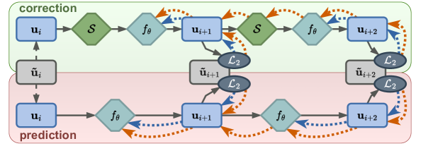
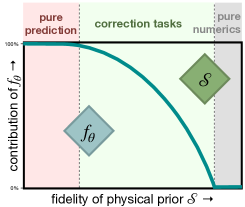
Figure 2: Left: Illustration of unrolling for a horizon $m=2$ for correction and prediction chains, including gradient flow in the backward pass for non-differentiable (blue, NOG) and differentiable (orange, WIG) setups, note how the gradients do not flow through a time step for NOG; Right: Contributions of networks and numerical solvers in prediction and correction paradigms

4 Physical Systems and Architectures

Four physical systems were used for our learning tests. All systems are parameterized to exhibit varying behavior, and each test set contains unseen values inside and outside the range of the training data set.

4.1 Kuramoto-Sivashinsky

This equation is a fourth-order chaotic PDE. The domain size, which leads to more chaotic behavior and shorter Lyapunov times for larger values [15], was varied across training and test data sets. The ground truth solver uses an exponential RK2 integrator [12]. In order to create a challenging learning scenario, the base solver for correction resorts to a first-order version that diverges within 14 steps on average. We base most of our empirical tests on this Kuramoto-Sivashinsky (KS) case since it combines challenging learning tasks with a small computational footprint. The KS equation is a fourth-order stiff PDE governed by

$$\frac{\partial u}{\partial t}+u\frac{\partial u}{\partial x}+\frac{\partial^{2}u}{\partial x^{2}}+\frac{\partial^{4}u}{\partial x^{4}}=0,$$ (12)

with simulation state $u$, time $t$, and space $x$ living in the domain of size $\mathcal{X}$. The dynamics exhibit a highly chaotic behavior. The domain was discretized with 48 grid points, and timesteps were set to $1$. The physical domain length $\mathcal{X}$ is the critical parameter in the KS equation. The training dataset was computed for a range of $\mathcal{X}=2\pi*[5.6,6.4,7.2,8,8.8,9.6,10.4]$. A sequence of $5000$ steps was computed for each domain length. The numerical solves and network training were performed in PyTorch [45].

Neural Network Architectures:

We use two architectures for learning tasks with the KS case: a graph-based (GCN) and a convolutional network (CNN). Both networks follow a ResNet-like structure [23], have an additive skip connection from input to output, and are parameterized in terms of their number of features per message-passing step or convolutional layer, respectively. They receive 2 channels as input, a normalized domain size $\mathcal{X}$ and $u$, and produce a single channel, the updated $u$, as output. The GCN follows the hierarchical structure of directional Edge-Conv graph nets [63, 31] where each Edge-Conv block is comprised of two message-passing layers with an additive skip connection. The message-passing concatenates node, edge, and direction features, which are fed to an MLP that returns output node features. At a high level, the GCN can be seen as the message-passing equivalent of a ResNet. These message-passing layers in the GCN and convolutional layers in the CNN are scaled in terms of whole ResBlocks, i.e., two layers with a skip connection and leaky ReLU activation. The networks feature additional linear encoding and decoding layers for input and output. The architectures for GCN and CNN were chosen such that the parameter count matches, as listed in table 2.

Table 2: KS Network Architectures and Parameter Counts; we denote the number of blocks as network depth, and specify the network architectures with a tuple containing (features, depth); For both GCN and CNN the smallest network size with a depth indicated by ”-” is a special case using a single non-linear layer with the listed number of features.

Architecture:	.5k*	.5k	2k	33k	.2M	1M
GCN (features, depth):	(46,-)	(9,1)	(14,2)	(31,8)	(63,12)	(126,16)
GCN Parameters:	511	518	2007	33,578	198,770	1,037,615
CNN (features, depth):	(48,-)	(8,1)	(12,2)	(26,8)	(52,12)	(104,16)
CNN Parameters:	481	481	1897	33125	196457	1042705

Hence, this represents the smallest possible architecture for our chosen range of architectures, consisting of a linear encoding, one non-linear layer followed by a linear decoding layer.

Network Training:

Every network was trained for a total of $50000$ iterations of batchsize $16$. The learning rate was initially set to $1\times 10^{-4}$, and a learning rate decay of factor $0.9$ was deployed after every $2000$ iterations during training. The KS systems was set up to quickly provide substantial changes in terms of simulated states. As a consequence, short unrollments of $m=3$ were sufficient during training unless otherwise mentioned. For this unrollment number, no curriculum was necessary.

For fairness across the different training variants the KS setup additionally keeps the number of training data samples constant for ONE versus NOG and WIG. For the latter two, unrolling means that more than one state over time is used for computing the learning gradient. Effectively, these two methods see $m$ times more samples than ONE for each training iteration. Hence, we increased the batch size of ONE training by a factor of $m$. However, we found that this modification does not result in an improved performance for ONE in practice.

For the tests shown in figure 8 of the main paper we varied the training data set size, reducing the number of time steps in the training data set to $1000$, while keeping the number of training iterations constant. The largely unchanged overall performance indicates that the original data set could be reduced in size without impeding the performance of the trained models.

Network Evaluation:

We computed extra- and interpolative test sets for the domain length $\mathcal{X}$. The extrapolation uses $\mathcal{X}=2\pi*[4.8,11.2]$, whilst interpolation is done for $\mathcal{X}=2\pi*[6.8,9.2]$. For our $\mathcal{L}_{2}$ results, we initialized autoregressive runs with 20 initial conditions for each $\mathcal{X}$, accumulated the $\mathcal{L}_{2}$ for sequences of $40$ steps, and averaged over all extra- and interpolative cases. The standard deviation is computed over the total set of tests. The time until decorrelation was calculated by running an autoregressive inference sequence. The steps were counted until the cross-correlation between the inferred state and the reference dropped below $0.8$. The statistics of the reached step-counts were gathered over all test cases, just like for the $\mathcal{L}_{2}$. The divergence time was defined as the number of inference steps until $\mathcal{L}_{2}>500$. Again, statistics were gathered over all test cases.

4.2 Wake Flow

Our second system is a two-dimensional flow around a cylinder, governed by the incompressible Navier-Stokes equations. The Wake Flow (WAKE) dataset consists of Karman-Vortex streets with varying Reynolds numbers, uses numerical solutions of the incompressible Navier-Stokes equations

$$\begin{split}\frac{\partial\mathbf{u}}{\partial t}+(\mathbf{u}\cdot\nabla)\mathbf{u}&=-\nabla p+\frac{1}{Re}\nabla^{2}\mathbf{u}+\mathbf{f},\\ \nabla\cdot\mathbf{u}&=0,\end{split}$$ (13)

with the two-dimensional velocity field $\mathbf{u}$ and pressure $p$, and an external forcing $\mathbf{f}$ which is set to zero in this case.

Numerical Data

The ground truth data was simulated with operator splitting using a Chorin-projection for pressure and second-order semi-Lagrangian advection [8, 17]. The training data is generated with second-order advection, while learning tasks use a truncated spatial resolution ($4\times$), and first-order advection as a correction base solver. Simulations were run for a rectangular domain with a 2:1 side aspect ratio, and a cylindrical obstacle with a diameter of $L_{D}=0.1$ placed at $(0.5,0.5)$ with a constant bulk inflow velocity of $U=1$. The Reynolds number is defined as $Re=\frac{UL_{D}}{\nu}$. The physical behavior is varied with the Reynolds number by changing the viscosity of the fluid. The training data set contains 300 time steps for six Reynolds numbers $Re=[97.5,195,390,781.25,1562.5,3125]$ at resolution $[256,128]$. For learning tasks, these solutions are down-sampled by $4\times$ to $[64,32]$. The solver for the correction uses the same solver with a more diffusive first-order advection step. The numerical solves and network training were performed in PyTorch [45].

Neural Network Architectures:

This test case employs fully-convolutional residual networks [23]. The architectures largely follow the KS setup: the neural networks have a ResNet structure, contain an additive skip connection for the output, and use a certain number of ResBlocks with a fixed number of features. The smallest network uses 1 ResBlock with 10 features, resulting in 6282 trainable parameters. The medium-sized network has 10 ResBlocks with 16 features and 66,178 parameters, while the large network has 20 blocks with 45 features resulting in more than 1 milllion (1,019,072) parameters.

Network Training and Evaluation:

The networks were trained for three steps with 30000 iterations each, using a batch size of 3 and a learning rate of $1\times 10^{-4}$. The training curriculum increases the number of unrolled steps (parameter $m$ of the main text) from $m=1$, to $m=4$ and then $m=16$. Each stage applies learning rate decay with a factor of $1/10$. $\mathcal{L}_{2}$ errors are computed and accumulated over 110 steps of simulation for 12 test cases with previously unseen Reynolds numbers: three interpolative ones $Re=[2868.5,2930,2990]$ and nine extrapolative Reynolds numbers $Re=[3235,3174,3296,3845,3906,3967,4516.5,4577.5]$.

4.3 Kolmogorov Turbulence

Thirdly, we study a periodic two-dimensional Kolmogorov Flow (KOLM) [21] also following the incompressible Navier-Stokes equations. The additive forcing causes the formation of a shear layer, whose instability onset develops into turbulence [21]. The forcing was set to $\mathbf{f}=[\sin(k_{x}*y),\>0]^{T}$ with wavenumber $k_{x}=6$.

Numerical data:

The two-dimensional KOLM system is also governed by the incompressible Navier-Stokes equations, with the addition of a forcing term $\mathbf{f}$. We use a more involved semi-implicit numerical scheme (PISO by [26]) for this setup. Similarly to the WAKE system, the KOLM learning cases are based on a spatiotemporal resolution truncation with a ratio of $4\times$ in both space and time, and the Reynolds number is varied across training and test cases. The physical domain size was set to $L_{x}=L_{y}=2\pi$ and discretized by a $128\times 128$ grid. The timestep was set to $\Delta\tilde{t}=0.005$ for the high-resolution ground truth dataset, which maintained a Courant number smaller than $0.5$. The training dataset is based on a Reynolds number variation of $Re=[300,400,500,700,800,900]$. For each Reynolds number, $6000$ frames were added to the dataset. The numerical solves and network training were performed in Tensorflow [1].

Neural Network Architectures:

The KOLM networks are also based on ResNets. In each ResNet block, data is processed through convolutions and added to a skip connection. In contrast to KS and WAKE architectures, the number of features varies throughout the network. Four different network sizes were deployed, details of which are listed in Table 3. The network sizes in the KOLM case range from $32$ thousand to $1$ million.

Table 3: KOLM Network Architectures and Parameter Counts

Architecture	# Parameters	# ResNet Blocks	Block-Features
CNN, 32k	32369	5	[8, 20, 30, 20, 8]
CNN, 0.1M	115803	7	[8, 16, 32, 64, 32, 16, 8]
CNN, 0.5M	461235	7	[16, 32, 64, 128, 64, 32, 16]
CNN, 1M	1084595	9	[16, 32, 64, 128, 128, 128, 64, 32, 16]

Network Training and Evaluation:

A spatiotemporal downsampling of the ground truth data formed the basis of the training trajectories. Thus, training operated on a $4\times$ downsampled resolution with $4$ times larger time-steps, i.e. $32\times 32$ grid with $\Delta t=0.02$. The networks were trained with a curriculum that incrementally increased the number of unrolled steps such that $m=[1,2,4]$, with an accompanying learning rate schedule of $[10^{-4},10^{-5},10^{-6}]$. Additionally, a learning rate decay with factor $0.9$ after an epoch of $36$ thousand iterations. For each $m$, 144 thousand iterations were performed. The batch size was set to $1$.

$\mathcal{L}_{2}$ errors are computed and accumulated over 250 steps of simulation for 5 test cases with previously unseen Reynolds numbers: $Re=600$ for interpolation and $Re=1000$ for extrapolation.

Compressible Aerofoil flow (AERO):

In the final physical system, we investigate compressible flow around an aerofoil, a task centered on pure prediction. We utilize the open-source structured-grid code CFL3D [50, 49] to solve the compressible Navier-Stokes equations, thus generating our ground truth dataset. Here, we vary the Mach number while keeping the Reynolds number constant. Details of this system are found in appendix B.

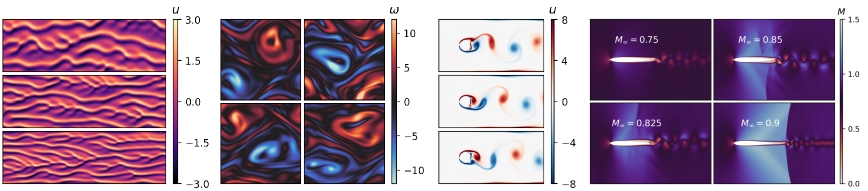
Figure 3: Visualizations of our physical systems, from left to right: KS equation state over time, KOLM vorticity field, WAKE vorticity field, AERO local Mach number field visualization for different upstream Mach numbers M_∞

5 Results

Our results compare the three training methods ONE, NOG, and WIG in various scenarios. The figure titles mark the physical system, whilst subscripts represent the network architecture (graph: graph network, conv: convolutional ResNet), and superscripts differentiate between correction (corr) and prediction (pred) tasks. For each test, we train multiple models (typically 8 to 20) for each setup that differ only in terms of initialization (i.e. random seed). The evaluation metrics were applied independently for outputs generated by each of the models, which are displayed in terms of mean and standard deviations below. This indicates the expected performance of a training setup and the reliability of obtaining this performance. A Welch’s test for statistical significance was performed for the resulting test distributions, and p-values can be found alongside the tabulated data in E.

5.1 Distribution Shift and Long-term Gradients

Agnosticisms

We first focus on establishing a common ground between the different variants by focusing on correction tasks for the physical systems. Training over 400 models with different architectures, initialization, and parameter counts, as shown in figure 4, reveals a first set of fundamental properties of training via unrolling: it reduces inference errors for graph- and convolutional networks, despite changes in dimensionality, the order of the PDE, and the baseline solver architecture. For the vast majority of tests, models trained with unrolling outperform the corresponding one-step baselines. Unrolling is also versatile concerning the type of the modeled correction, as networks were tasked to either learn truncations due to reduced convergence orders with graph networks (KS), or spatial grid coarsening errors via CNNs (KOLM, WAKE).

These findings are not new [3, 56], but confirm that our setup matches previous work. They already motivate recommendation (IV), i.e. that testing unrolled architectures can be performed efficiently on cheaper low-dimensional problems, such as the KS system.

Disentangling Contributions

Next, we investigate the effect of backpropagating gradients in the unrolled chain of network and simulator operations. The non-differentiable NOG setup already addresses the data shift problem, as it exposes the learned dynamics’ attractor at training time. The inference errors are visualized in figure 4. On average, training with NOG over ONE training yields an error reduction of 23%, in line with recommendation II. For large architectures, inference accuracy increases and learned and ground truth systems become more alike. In these cases, their attractors are similar, and unrolling is less crucial to expose the learned attractor. However, NOG training still uses crude gradient approximations, which negatively influences training regardless of how accurate the current model is. We believe this is why the NOG variant falls behind for large sizes. While NOG models remain closer to the target than ONE in all other cases, the results likewise show that the differentiable WIG setup further improves the performance. These networks reliably produce the best inference accuracy. Due to the stochastic nature of the non-linear learning processes, outliers exist, such as the $0.5$m NOG model of the KOLM system. Nonetheless, the WIG models consistently perform best and yield an average improvement of 38% over the ONE baseline. This error average behavior matches best-performing networks’ behavior (C).

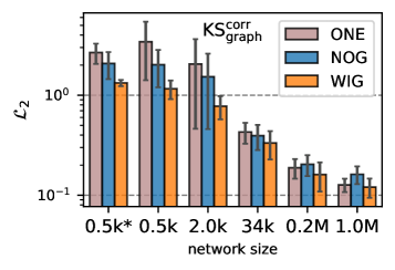
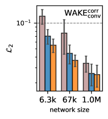
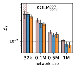
Figure 4: Inference accuracy measured in $\mathcal{L}_{2}$ for correction setups on KS, KOLM, and WAKE systems; displayed models were trained with ONE(brown), NOG(blue), WIG(orange); across network architectures (graph networks for KS, conv-nets otherwise

), and network sizes WIG has lowest errors; one 32k ONE model diverged in the KOLM case that NOG and WIG kept stable

Figure 5 depicts the time until de-correlation between inference runs and the ground truth for the KS system. For all model sizes and both network architectures, WIG achieves the longest inference rollouts until the de-correlation threshold is reached. Similarly to the observations on the $\mathcal{L}_{2}$ metric in Figure 4, NOG is the second best option for small and medium-sized networks when it comes to correlation. This observation again translates between the network architectures.

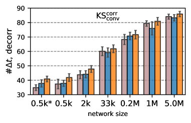
Figure 5: Number of timesteps until the threshold is reached for de-correlation

In addition, we studied the time until divergence for the KS system. This metric sets a high threshold of $\mathcal{L}_{2}>500$, which would correspond to a hundred-fold increase in the state of a simulation. This metric measures the time until the solution blows up, not whether there is a particular similarity to the ground truth. As such, a large number of timesteps can be seen as a metric for the autoregressive stability of the network. Figure 6 shows this evaluation for the KS system. The unrolled setups excel at this metric. Unsurprisingly, mitigating the data shift by unrolling the training trajectory stabilizes the inference runs. Through unrolling, the networks were trained on inference-like states. The most stable models were trained with the WIG setup, whose long-term gradients further discourage unphysical outputs that could lead to instabilities in long inference runs. The large networks’ divergence time comes close to the upper threshold we evaluated, i.e. 1000 steps.

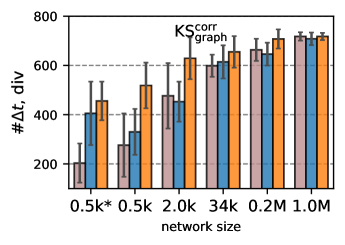
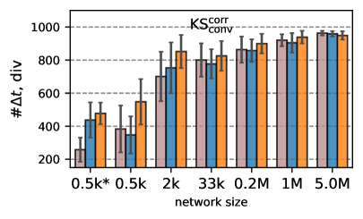
Figure 6: Number of timesteps until the threshold is reached for divergence

To conclude, our results allow for disentangling the influence of data shift and gradient divergence. As all training modalities, from data sets to random seeds, were kept constant, the only difference between NOG and WIG is the full gradient information provided to the latter. As such, we can deduce from our measurements that reducing the data shift contributes to the aforementioned improvement of 23%, while long-term gradient information yields another improvement of 15% (recommendation II). Figure 7 highlights this by depicting the accuracy of the unrolled setups normalized by the respective ONE setup for different model sizes and physical systems. WIG yields the best $L_{2}$ reductions. NOG in certain cases even performs worse with factors larger than one, due to its mismatch between loss landscape and gradient information, but nonetheless outperforms ONE on average. A crucial takeaway is that unrolling, even without differentiable solvers, provides measurable benefits to network training. As such, interfacing existing numerical codes with machine learning presents an attractive option that does not require the re-implementation of established solvers. Our results provide estimates for the expected gains with each of these options.

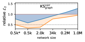
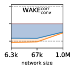
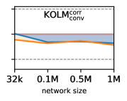
Figure 7: $\mathcal{L}_{2}$ error of NOG and WIG setups relative to the error achieved by ONE (i.e. ${\mathcal{L}^{\mathrm{NOG}}_{2}}/{\mathcal{L}^{\mathrm{ONE}}_{2}}$ and ${\mathcal{L}^{\mathrm{WIG}}_{2}}/{\mathcal{L}^{\mathrm{ONE}}_{2}}$); WIG training reliably produces more accurate results than NOG and ONE

Unrolling horizons

The effects of unrolling on data shift and gradient divergence depend on the unrolled length $m$, as summarized in Fig. 1. A long horizon diminishes the data shift, as the learned dynamics can be systematically explored by unrolling. At the same time, gradient inaccuracy impairs the learning signal in the NOG case, while exploding gradients can have a similar effect for long backpropagation chains in the WIG setup. We test this hypothesis by varying the unrolled training horizon. The results are visualized in figure 8. For increasing horizons, the inference performance of NOG variants improves until a turning point is reached. After that, NOG performance deteriorates quickly. In the following regime, the stopped gradients cannot map the information gained by further reducing the data shift to an effective parameter update. The quality of the learning signal deteriorates. This is mitigated by allowing gradient backpropagation through the unrolled chain in the WIG setup. Herein, the inference accuracy benefits from even longer unrollings, and only diverges for substantially larger $m$ when instabilities from recurrent evaluations start to distort the direction of learning updates. These empirical observations confirm the theoretical analysis that went into Figure 1: There exist unrolling horizons for which training performance is improved for both NOG and WIG, while this effective horizon is longer for WIG.

As training with long unrolling poses challenges, we found a curriculum-based approach with an incremental increase of the unrolling length $m$ at training time to be essential [56, 30]. Figure 8 shows how long unrollings in the initial training phases can hurt accuracy. Untrained networks are particularly sensitive since autoregressive applications can quickly lead to divergence of the simulation state or the propagated gradients. At the same time, learning rate scheduling is necessary to stabilize gradients (recommendation IV).

Gradient Stopping

Cutting long chains of gradients was previously proposed as a remedy for training instabilities of unrolling [37, 7, 54]. Discarding gradients for a number of initial steps [7, 47] is indicated by the parameter $w$ describing the number of warm-up steps for which gradients are stopped.

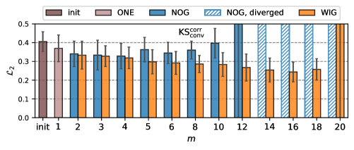
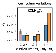
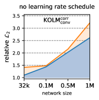
Figure 8: Left: variation of unrolling horizons $m$ trained for the KS system; all models were initialized with the leftmost ONE setup; with NOG training, the error increases and explodes for $m>6$; WIG remains stable for longer horizons, diverges at $m>18$; Middle: different curriculums for the KOLM system; starting the training with large $m$ leads to unfavorable network states; Right: Inference accuracy without learning rate schedule relative to with scheduling, i.e. $\mathcal{L}_{2}^{\mathrm{no-schedule}}/\mathcal{L}_{2}^{\mathrm{schedule}}$; All models benefit from learning rate scheduling, indicated by values are larger than one, and especially for larger models the schedule is crucial

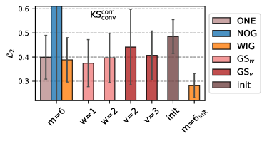
Figure 9: Gradient stopping techniques

As shown in Fig. 9, setting $w$=1 can yield mild improvements over training over the full chain if no curriculum is used. Dividing the backpropagation into subsections [37] likewise does not yield real improvements in our evaluation. We divided the gradient chain into two or three subsections, identified by the parameter $v$ in Fig. 9.

The best performance is obtained with the full WIG setup and curriculum learning, where unrolled models are pre-trained with $m$=1 models. This can be attributed to the more accurate gradients of WIG, as all gradient-stopping variants above inevitably yield a mismatch between loss landscape and learning updates (recommendation II).

Network Scaling

Figure 4 shows clear, continuous improvements in accuracy for increasing network sizes. An obvious conclusion is that larger networks achieve better results. However, in the context of scientific computing, arbitrarily increasing the network size is not admissible. As neural approaches compete with established numerical methods, applying pure neural or hybrid architectures always entails accuracy, efficiency, and scaling considerations. The scaling of networks towards large engineering problems on physical systems has been an open question. Figure 10 estimates the convergence rate of the correction networks with respect to the parameter count to be $n^{-{1}/{3}}$. Interestingly, the measured convergence rates are agnostic to the physical system and the studied network architectures. This convergence rate is poor compared to classic numerical solvers, and indicates that neural networks are best applied for their intrinsic benefits. They possess appealing characteristics like data-driven fitting, reduced modeling biases, and flexible applications. In contrast, scaling to larger problems is more efficiently achieved by numerical approaches. In applications, it is thus advisable to combine both methods to render the benefits of both components. In this light, our correction results for small and medium-sized networks have more relevance to potential applications. Therefore, the two main conclusions from this subchapter are as follows: Firstly, the solver part in hybrid architectures scales more efficiently than the neural network part. Secondly, it becomes apparent how network size dominates the accuracy metrics (recommendation III). Thus, parameter counts need to be equal when fairly comparing network architectures. Another observation is the lack of overfitting: despite the largest KS models being heavily overparameterized with five million parameters for a simulation with 48 degrees of freedom accuracy still improves. This finding aligns with recent insights on the behavior of modern large network architectures [5].

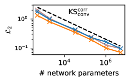
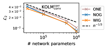
Figure 10: Accuracy convergence over network size, correction networks converge with $n^{-1/3}$

5.2 Varied Learning Tasks

To broaden the investigation of the unrolling variants, we vary the learning task by removing the numerical solver from training and inference. This yields prediction tasks where the networks directly infer the desired solutions. Apart from this increased difficulty, all other training modalities were kept constant, i.e., we likewise compare non-differentiable NOG models to full unrolling (WIG).

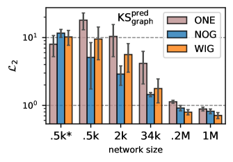
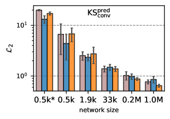
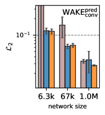
Figure 11: Prediction setups with inference accuracy measured in terms of $\mathcal{L}_{2}$ on KS and WAKE; NOG performs well for small network sizes, while WIG is show advantages for larger ones

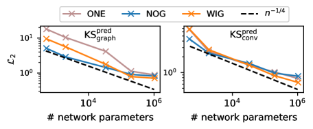
Figure 12: Accuracy convergence over network size, prediction converges with $n^{-1/4}$

Prediction

The parameter count of models still dominates the accuracy but in contrast to before, the NOG setup performs better than both alternatives for smaller network sizes. This is shown in Fig. 11. The inference errors for the prediction setup are roughly an order of magnitude larger than the respective correction errors. This indicates that pure predictions more quickly diverge from the reference trajectory, especially for small network sizes. The deteriorated performance of WIG can be explained by these larger differences between the inferred state and the references, leading to suboptimal gradient directions. For the setups in Figure 11, NOG training achieves improvements of 31%, and WIG improves on this by a further 3.6%. In general, unrolling maintains strong benefits in prediction setups, but differentiability is less benefitial than in correction setups.

Smooth Transition

While the learning task is typically mandated by the application, our setup allows us to investigate the effects of unrolling for a smooth transition from prediction to increasingly simple correction tasks, in line with Fig. 2. In the pure prediction case, the physical prior does not model any physics, i.e., is an identity operator. We transition away from pure predictions by providing the network with improving inputs by increasing the time step of the reference solver for correction tasks. On the other end of the spectrum the numerical solver computes the full time step, and the neural network now only has the trivial task to provide an identity function. Since the total error naturally decreases with simpler tasks, figure 13 shows the performance normalized by the task difficulty. The positive effects of NOG and especially WIG training carry over across the full range of tasks. Interestingly, the NOG version performs best for very simple tasks on the right sides of each graph. This is most likely caused by a relatively small mismatch of gradients and energy landscape. In our experiments, the task difficulty was changed by artificially varying the prior’s accuracy. This mimics the effects of basing the correction setups on different numerical schemes. Since unrolling manifests a stable performance improvement across all priors, it promises benefits for many correction setups in other applications. The results above indicate that a 5x accuracy boost can be achieved by integrating low-fidelity physics priors in a NOG setup.

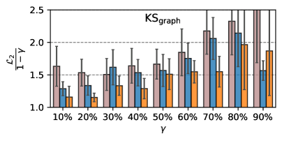
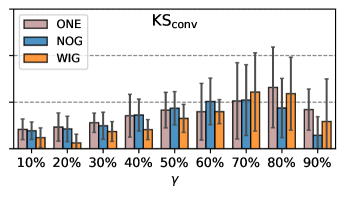
Figure 13: Transition from prediction to correction; a smooth transition in modeling difficulty is achieved by varying the timestep of the numerical solver embedded in the correction step $\gamma=\Delta t_{\mathcal{S}}/\Delta\tilde{t}$, with the solver timestep $\Delta t_{\mathcal{S}}$ and the ground truth timestep $\Delta\tilde{t}$

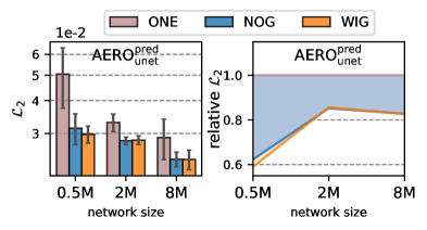
Figure 14: Left: Prediction of the AERO system, absolute errors of ONE, NOG, and WIG; Right: Relative errors with respect to ONE

Changing the Physical System

The AERO dataset comprises aerofoil flows in the transonic regime and features shocks, fast-changing vorticial structures, and diverse samples around the critical $\text{Ma}=0.8$. As such, we deployed a modern attention-based U-Net [44]. As a complex, large-scale test scenario, our learning setups for the AERO system implement the recommendations we derived from the previous results. Figure 14 shows the inference evaluation of our trained models. Once again, unrolling increases accuracy at inference time. On average, unrolling improves the inference loss by up to 32% in the AERO case. The results reflect our recommendations: Network size has the largest impact, and choosing the right size balances performance and accuracy (III). Additionally, our models were trained with a learning rate scheduled curriculum to achieve the best results (V), details of which are found in Appendix B. Training on the AERO system resembles the behavior of lower-dimensional problems, e.g. the KS system (IV). Similar to our previous prediction tasks, long-term gradients are less crucial, but still deliver the best models (II). However, unrolling itself is essential for stable networks (I).

5.3 The Potential of No-Gradient Unrolling

Existing studies focus on fixed tasks, i.e. pure prediction tasks when no differentiable solver is available, and correction tasks when employing a differentiable solver. Given the large and complex implementations of solvers used in current scientific projects, often with decade-long histories, approaches that do not require the differentiability of these numerical solvers are especially attractive. Our experiments quantify the expected benefits when switching from a prediction task to a correction task with a non-differentiable solver.

As illustrated in figure 15, this enables an average 4.5-fold accuracy improvement with the same network architecture and size. Small architectures can especially benefit from training with NOG utilizing a non-differentiable physical prior. The models with 0.5k parameters perform 9.36 and 3.83 times better when supported by a low-fidelity solver, where the second value originates from a deeper variant of the 0.5k parameterization. The factor remains relatively constant for the remaining sizes, which all deploy deep architectures. Medium-sized networks with 2k and 33k parameters see a slight decrease in these improvements with values of 2.80 and 3.23 respectively, while the largest networks’ accuracies improve by a factor of 3.82 and 3.96 once trained with NOG in a correction setup. In the KOLM case, we observe similar relative gains from introducing a numerical solver as physical prior. Here, the factor is 4.8 on average. Again, this relative factor is largest for small architectures, where we observe a value of 6.2 for the 32k network. Similarly to the KS case, the benefits of using a physical prior decrease for larger architectures. For our KOLM experiments the values are 4.19, 4.88, and 4.19 respectively. It has to be noted that these factors likely are specific to our setups and the numerical solvers chosen as a prior. However, the purpose of this evaluation is to illustrate the potential improvements made possible by correction unrolling. Crucially, only an interface between the solver and the network is sufficient for NOG correction training, the core of the solver can remain untouched. These experiments indicate that there could be large benefits if scientific codes were interfaced with machine learning (recommendation I, III). We believe that this training modality could be a new common ground for machine learning and the computational sciences. In the past, machine learning focused works often focused on purely predictive tasks. As our results indicate, an interface with existing numerical architectures is not only necessary to deploy hybrid models in a scientific computing environment but additionally unlocks further accuracy improvements when models are trained with NOG unrolling.

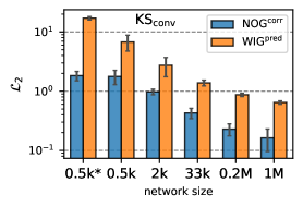
Figure 15: Comparison of WIG prediction and NOG correction setups on the KS system (left) and the KOLM flow (right)

6 Conclusion

We have conducted in-depth empirical investigations of unrolling strategies for training neural PDE simulators. The inherent properties of unrolling were deduced from an extensive test suite spanning multiple physical systems, learning setups, network architectures, and network sizes. Our findings rendered five best practices for training autoregressive neural simulators via unrolling. Additionally, our test sets and differentiable solvers are meant to serve as a benchmark: The broad range of network sizes for popular architectures as well as the selection of common physical systems as test cases yield a flexible baseline for future experiments with correction and prediction tasks. We have identified non-differentiable unrolling as an attractive alternative to simplistic one-step training and implementations of differentiable solvers. Our results lay the foundation for assessing potential gains by deploying this method. Lastly, we measured convergence rates for neural networks and saw how these architectures converge poorly compared to numerical solvers. We concluded that deploying neural networks may thus be beneficial when a particular problem can benefit from their inherent properties, while grid scaling is still more efficient with classical approaches.

In the future, problem-tailored network architectures could potentially improve the scaling of neural networks. However, at the current point of research, it is advisable to combine neural and numerical approaches in hybrid architectures to benefit from both. One of the applications that could benefit from this approach is training closure models for filtered or averaged PDE s. At the same time, there are limitations to our scope. Our physical systems live in the domain of non-linear chaos and are primarily connected to fluid mechanics. Consequently, there is no inherent guarantee that our results will straightforwardly transfer to different domains. Additionally, we mentioned the relevance of our results to the scientific computing community. Our recommendations can help prioritize implementation efforts when designing unrolled training setups. However, we have only studied a subset of the relevant hyperparameters. In the context of unrolling, variations such as network width and depth, advanced gradient-stopping techniques, and irregularly spaced curriculums could be impactful. These topics are promising avenues for future research to further our understanding of autoregressive neural networks for scientific applications.

Acknowledgements

This work was supported by the ERC Consolidator Grant SpaTe (CoG-2019-863850).

Code Availablility

The code for the project is available at https://github.com/tum-pbs/unrolling.

APPENDIX

Appendix A Gradient Calculation

A.1 Correction

The network parameter optimization was defined in Equation 5. For one learning iteration, a loss was accumulated over an unrolled trajectory. We can write this total loss over the unrolled trajectory as a function of $g(\mathbf{u}^{i})=f_{\theta}(\mathcal{S}(\mathbf{u}^{i}))$ such that

$$\mathcal{L}=\sum_{i=1}^{s}\mathcal{L}_{2}(\tilde{\mathbf{u}}^{i+\tau s},g^{s}(\mathbf{u}^{i}))=\sum_{i=1}^{s}\mathcal{L}^{s},$$ (14)

where $g^{s}$ represents the recurrent application of multiple machine learning augmented simulation steps, and $\mathcal{L}^{s}$ represents the loss evaluated after that step. Note that the full backpropagation through this unrolled chain requires a differentiable solver for the correction setup. To test the effect of using a differentiable solver, we introduce two different strategies for propagating the gradients $\frac{\partial\mathcal{L}_{u}}{\partial\theta}$. The differentiable setup can calculate the full optimization gradients by propagating gradients through the solver. The gradients are thus evaluated as

$$\frac{\partial\mathcal{L}^{s}}{\partial\theta}=\sum_{B=1}^{s}\bigg{[}\frac{\partial\mathcal{L}^{s}}{\partial g^{s}}\bigg{(}\prod_{b=1}^{s-B}\frac{\partial g^{s-b}}{\partial f_{\theta}^{s-b}}\frac{\partial f_{\theta}^{s-b}}{\partial\mathcal{S}^{s-b}}\frac{\partial\mathcal{S}^{s-b}}{\partial g^{s-b-1}}\bigg{)}\frac{\partial g^{B}}{\partial f_{\theta}^{B}}\frac{\partial f_{\theta}^{B}}{\partial\theta}\bigg{]}.$$ (15)

We refer to this fully differentiable setup as WIG. In contrast, if no differentiable solver is available, optimization gradients can only propagate to the network application, not through the solver. The gradients are thus evaluated as

$$\frac{\partial\mathcal{L}_{s}}{\partial\theta}=\frac{\partial\mathcal{L}_{s}}{\partial g^{s}}\frac{\partial g^{s}}{\partial f_{\theta}^{s}}\frac{\partial f_{\theta}^{s}}{\partial\theta}.$$ (16)

This setup is referred to as NOG. Most existing code bases in engineering and science are not fully differentiable. Consequentially, this NOG setup is particularly relevance, as it could be implemented using existing traditional numerical solvers.

A.2 Prediction

Prediction operates on the same network parameter optimization from Equation 5. The total loss over the unrolled trajectory is

$$\mathcal{L}=\sum_{i=1}^{s}\mathcal{L}_{2}(\tilde{\mathbf{u}}^{i+\tau s},f_{\theta}^{s}(\mathbf{u}^{i}))=\sum_{i=1}^{s}\mathcal{L}^{s},$$ (17)

where $f_{\theta}^{s}$ represents the recurrent application of the network and $\mathcal{L}^{s}$ represents the loss evaluated after that step. To test the effect of using long-term gradients, we introduce two different strategies for propagating the gradients $\frac{\partial\mathcal{L}_{u}}{\partial\theta}$. The differentiable setup can calculate the full optimization gradients by propagating gradients through the solver. The gradients are thus evaluated as

$$\frac{\partial\mathcal{L}^{s}}{\partial\theta}=\sum_{B=1}^{s}\bigg{[}\frac{\partial\mathcal{L}^{s}}{\partial f_{\theta}^{s}}\bigg{(}\prod_{b=1}^{s-B}\frac{\partial f_{\theta}^{s-b}}{\partial f_{\theta}^{s-b-1}}\bigg{)}\frac{\partial f_{\theta}^{B}}{\partial\theta}\bigg{]}.$$ (18)

We refer to this fully differentiable setup as WIG. In contrast, if no differentiable solver is available, optimization gradients can only propagate to the network application, not through the solver. The gradients are thus evaluated as

$$\frac{\partial\mathcal{L}_{s}}{\partial\theta}=\frac{\partial\mathcal{L}_{s}}{\partial f_{\theta}^{s}}\frac{\partial f_{\theta}^{s}}{\partial\theta}.$$ (19)

This setup is referred to as NOG. Most existing code bases in engineering and science are not fully differentiable. Consequentially, this NOG setup is particularly relevance, as it could be implemented using existing traditional numerical solvers.

Appendix B AERO case

Numerical data:

The governing equations for the transonic flow over a NACA0012 airfoil are non-dimensionalized with the freestream variables (i.e., the density $\rho_{\infty}$, speed of sound $a_{\infty}$, and the chord length of the airfoil $c$), and can be expressed in tensor notation as

$$\begin{split}\frac{\partial\rho u_{\mathrm{i}}}{\partial x_{\mathrm{i}}}=0\\ \frac{\partial\rho u_{\mathrm{i}}u_{\mathrm{j}}}{\partial x_{\mathrm{j}}}=-\frac{\partial p}{\partial x_{\mathrm{i}}}+\frac{\partial\tau_{x_{\mathrm{i}}x_{\mathrm{j}}}}{\partial x_{\mathrm{j}}}\\ \frac{\partial(\rho E+p)u_{\mathrm{i}}}{\partial x_{\mathrm{i}}}=\frac{\partial(-q_{\mathrm{i}}+u_{\mathrm{j}}\tau_{x_{\mathrm{i}}x_{\mathrm{j}}})}{\partial x_{\mathrm{i}}}\end{split}$$ (20)

where the shear stress (with Stokes’ hypothesis) and heat flux terms are defined as

$$\tau_{x_{\mathrm{i}}x_{\mathrm{j}}}=\mu\frac{M_{\infty}}{Re_{\infty}}[(\frac{\partial u_{\mathrm{i}}}{\partial x_{\mathrm{j}}}+\frac{\partial u_{\mathrm{j}}}{\partial x_{\mathrm{i}}})-\frac{2}{3}\frac{\partial u_{\mathrm{k}}}{\partial x_{\mathrm{k}}}\delta_{\mathrm{i}\mathrm{j}}]$$

and

$$q_{x_{\mathrm{i}}}=-\frac{\mu}{Pr}\frac{M_{\infty}}{Re_{\infty}(\gamma-1)}\frac{\partial\Theta}{\partial x_{\mathrm{i}}}.$$

Here, Reynolds number is defined as $Re_{\infty}=\rho_{\infty}\sqrt{u_{\infty}^{2}+v_{\infty}^{2}}c/\mu_{\infty}$; $\gamma$ is the ratio of specific heats, 1.4 for air; the laminar viscosity $\mu$ is obtained by Sutherland’s law (the function of temperature), and the turbulent viscosity $\mu_{T}$ is determined by turbulence models; laminar Prandtl number is constant, i.e. $Pr=0.72$. The relation between pressure $p$ and total energy $E$ is given by

$$p=(\gamma-1)\bigl{[}\rho E-\frac{1}{2}\rho u_{\mathrm{i}}u_{\mathrm{i}}\bigr{]}.$$

Note also that from the equation of state for a perfect gas, we have $p=\rho a^{2}/\gamma$ and temperature $\Theta=a^{2}$. As we perform 2D high-resolution quasi-direct numerical simulations, no turbulence model is employed.

The finite-volume method numerically solves the equations using the open-source code CFL3D. The mesh resolution $1024\times 256$ is kept the same for cases, i.e. 256 grid cells in the wall-normal direction, 320 grid cells in the wake, and 384 grid cells around the airfoil surface. The convective terms are discretized with third-order upwind scheme, and viscous terms with a second-order central difference.

An inflow/outflow boundary based on one-dimensional Riemann invariant is imposed at about 50c away from the airfoil in the (x, y) plane. The grid stretching is employed to provide higher resolution near the surface and in the wake region, and the minimal wall-normal grid spacing is $6\times 10^{-4}$ to ensure $y^{+}_{n}<1.0$. A no-slip adiabatic wall boundary condition is applied on the airfoil surface. The non-dimensional time step is $0.008c/{U_{\infty}}$.

In the transonic regime, airflow behavior becomes more complex due to the formation of shock waves and supersonic and subsonic flow areas on the airfoil surfaces. When the Mach number is below $M=0.77$, the unsteadiness in the flowfield is mainly caused by the high-frequency vortex shedding. At around $M=0.8$, a series of compression waves coalesce to form a strong shock wave, and the flow structures are dominated by alternately moving shock waves along the upper and lower sides of the airfoil. For $M>0.88$, the strong shock waves become stationary on both surfaces. To cover all possible flow regimes, the samples in the training dataset are generated at $M=[0.75,0.8,0.825,0.88,0.9]$, and the test samples are performed at $M=0.725$ and $M=0.775$.

The snapshots are saved at every four simulation steps (i.e., $dt_{sampling}=0.032c/U_{\infty}$) and spatially downsampled by 4x and 2x in the circumferential and wall-normal directions, respectively. In the case of $M=0.85$, there are 1000 snapshots; for other cases, there are 500 snapshots.

Neural Network Architectures:

We implemented Attention U-Net [44]. It consists of three encoder blocks, each progressively capturing features from the input image through convolution and downsampling. Following the encoder blocks, there’s a bottleneck block for information compression with a higher number of channels. Subsequently, the architecture includes three decoder blocks, which use skip connections to integrate features from both the bottleneck and corresponding encoder blocks during the upscaling process. These decoder blocks gradually reduce the number of channels, culminating in a 1x1 convolutional output layer that generates pixel-wise predictions. We train networks of varying sizes by adjusting the number of features, as indicated in Table 4. The training was performed in PyTorch [45].

Table 4: AERO Network Architectures and Parameter Counts

Architecture	# Parameters	Features in encoder & bottleneck blocks
UNet, 0.5m	511332	[16, 32, 64] [128]
UNet, 2.0m	2037956	[32, 64, 128] [256]
UNet, 8.1m	8137092	[64, 128, 256] [512]

Network Training and Evaluation

The model is trained with Adam and a mini-batch size of 5, with training noise, for up to 500k iterations. A learning rate of $6\times 10^{-4}$ is used for the first 250k iterations and then decays exponentially to $6\times 10^{-5}$. The training curriculum increases the number of unrolled steps from $m=1$ to $m=4$ and then $m=9$.

$\mathcal{L}_{2}$ errors are computed and accumulated over 200 prediction steps (equivalent to 800 simulator steps) of simulation for two test cases with previously unseen Mach numbers: $M=0.725$ and $M=0.775$, corresponding to shock-free case and near-critical condition case.

Appendix C Additional Results

C.1 Prediction on the KOLM system

The networks used for the correction of the KOLM system were also trained for prediction. The results are visualized in figure 16. Unsurprisingly, the overall error values are larger than for the respective correction setups, where an additional numerical prior supports the network. Like the other prediction and correction setups, the errors decrease with increasing network size. Unrolled training modalities perform best at all network sizes. The quantitative values of the loss metric are also tabulated in 12.

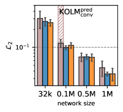
Figure 16: Comparison of $\mathcal{L}_{2}$ errors for CNN predictions on the KOLM flow

C.2 Interpolation and Extrapolation Tests

Interpreting physical hyperparameters is necessary for models to generalize to extrapolative test cases. We want to test whether extrapolation to new physical hyperparameters benefits from unrolling or long term gradients. In the main sections, all evaluations accumulated their results from interpolative and extrapolative test cases. In this section, we explicitly differentiate between interpolation and extrapolation tests. Figures 17, 18, 19, and 20 compare the model performance on interpolative and extrapolative test cases with respect to the physical parameters and depicts performance relative to the ONE baseline for various model sizes. Overall accuracy is worse on the harder extrapolative test cases. Similarly to the combined tests from the main section WIG performs best on average, both on interpolative or extrapolative data. However, the long-term gradients introduced by this method do not seem to explicitly favor inter- or extrapolation. Nonetheless, the positive aspects of WIG training are not constrained to interpolation, but successfully carry over to extrapolation cases.

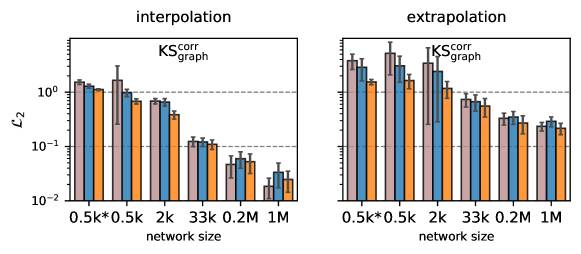
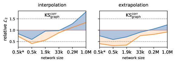
Figure 17: Comparison of $\mathcal{L}_{2}$ errors on interpolative and extrapolation test sets for GCNs on KS

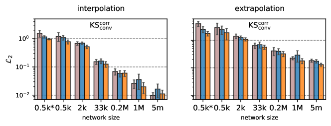
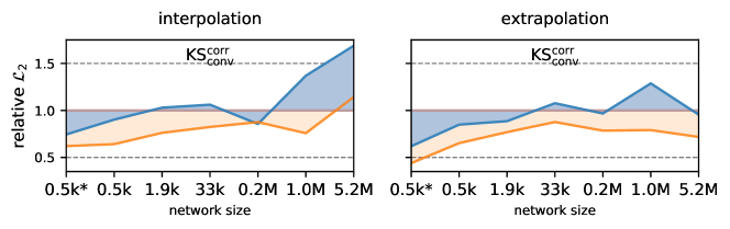
Figure 18: Comparison of $\mathcal{L}_{2}$ errors on interpolative and extrapolation test sets for CNNs on KS

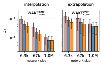
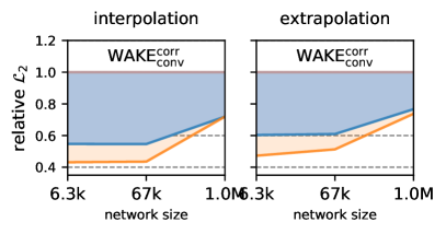
Figure 19: Comparison of $\mathcal{L}_{2}$ errors on interpolative and extrapolation test sets for WAKE

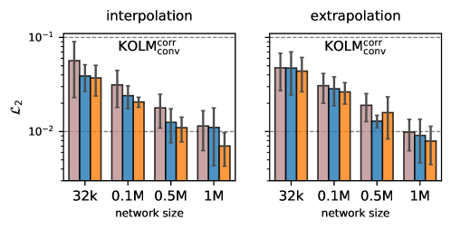
Figure 20: Comparison of $\mathcal{L}_{2}$ errors on interpolative and extrapolation test sets for KOLM

C.3 Dataset Sizes

Unrolling connects multiple dataset frames in one trajectory. This connectedness encodes the physical relation between subsequent frames that ultimately has to be learned by the neural network. Given that unrolled setups observe more of these physical connections, one might expect that unrolling decreases the necessary dataset size. To test this hypothesis, we incrementally decreased the amount of training data. The number of training iterations was kept constant throughout the process. The models are then evaluated on our full test sets. Figure 21 compares the $\mathcal{L}_{2}$ for variations in the training dataset size. A measurable difference in inference accuracy only appears for dataset sizes smaller than $X\%$ of the original dataset. While the accuracy of WIG does indeed deteriorate slightly later than NOG and especially ONE, this transition is confined to a small section of $Y\%$ dataset size. In practice, training a setup in this narrow dataset margin is unlikely and thus not mentioned as a strong benefit of unrolling.

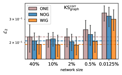
Figure 21: Dataset size variations in percent of the full training set

C.4 Best performing models

Our error measurements relied on statistical evaluations, which in turn were based on multiple randomized training runs. NOG and especially WIG showed clear benefits in these statistical evaluations. However, we must also consider the computational cost of training (differentiable) unrolled setups. Unrolling $m$ steps with the NOG setup increases the computational cost of one training iteration $m$-fold. Differentiable training in the WIG setup adds even more computations due to the backpropagation through the solver. Consequently, training multiple models and selecting the best might be a viable approach for ONE models, where training costs are lower. Thus, we evaluate the best-performing models in a separate analysis. Figure 22 depicts the best inference $\mathcal{L}_{2}$ achieved by a given model size, architecture, and learning setup. The best ONE models are on par with NOG or WIG for some network sizes and architectures. However, in many other cases, the average unrolled WIG setup still performs better or similar to the best ONE model. In light of the fact that these best models were selected out of 8 (KOLM) or 20 (KS) training runs, training with unrolling is ultimately more resource-efficient if best performance is sought. Thus, our recommendation of training with NOG or WIG approaches persists.

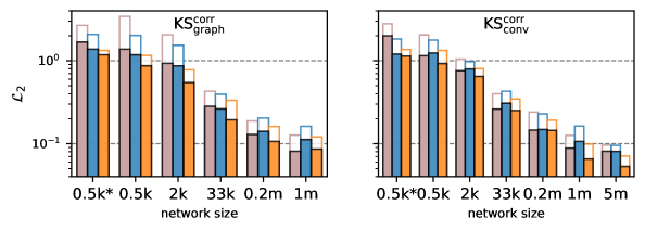
Figure 22: $\mathcal{L}_{2}$ errors of the best performing models; the outline in the background represent the average accuracy

C.5 Additional Architecture

Figure 23: Comparison of $\mathcal{L}_{2}$ errors for the U-Net architecture on the KS system

We tested the generalization of our findings toward attention-gated U-nets [44]. The implementation is a 1D version of the network used in the AERO cases introduced in Appendix B. Crucially, it features attention gates in its skip connections allowing the network to efficiently mix global and local structures in the output. The $\mathcal{L}_{2}$ errors of this architecture on the KS system are visualized in Figure 23. The behavior of ONE, NOG, and WIG matches well with other architectures (i.e. conv and graph nets) studied in the main section. We still observe the best performance with fully differentiable WIG unrolling, while NOG offers slimmer benefits over ONE. We can conclude that our observations regarding the positive effects of unrolling with and without gradients transfer to attention-based networks.

Appendix D Inference Visualizations

This section visualizes typical inference trajectories on which our evaluations were based. Due to the vast amount of trained models, only a very small subset of all models are visualized. The goal is to contextualize the results from the main paper and previous appendix evaluations. The following figures show various training modalities for a fixed initialization, which was randomly selected from our trained models.

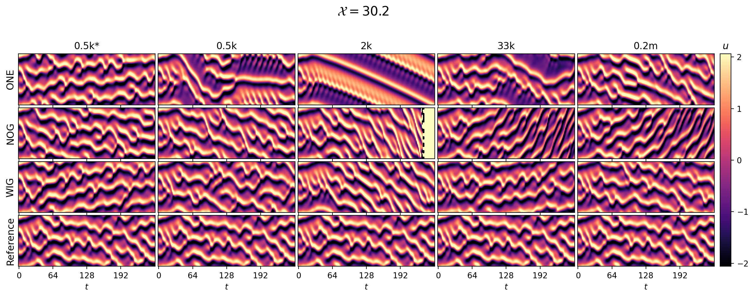
Figure 24: Inference error trajectory visualization of the CNN correction on the KS system for extrapolation on low $\mathcal{X}$

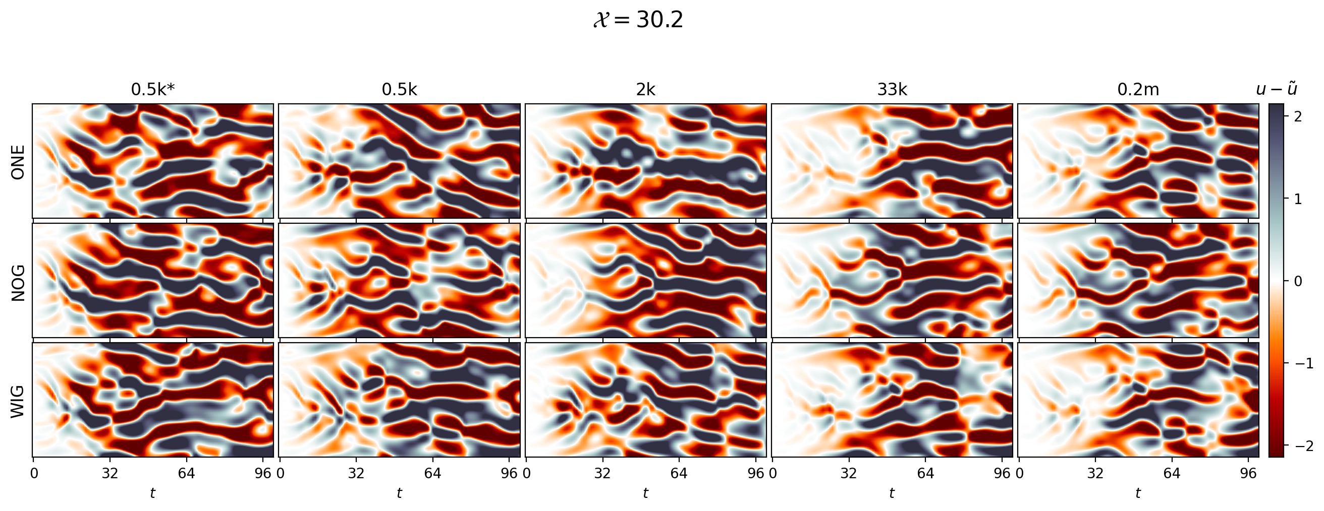
Figure 25: Inference error trajectory visualization of the CNN correction on the KS system for extrapolation on high $\mathcal{X}$

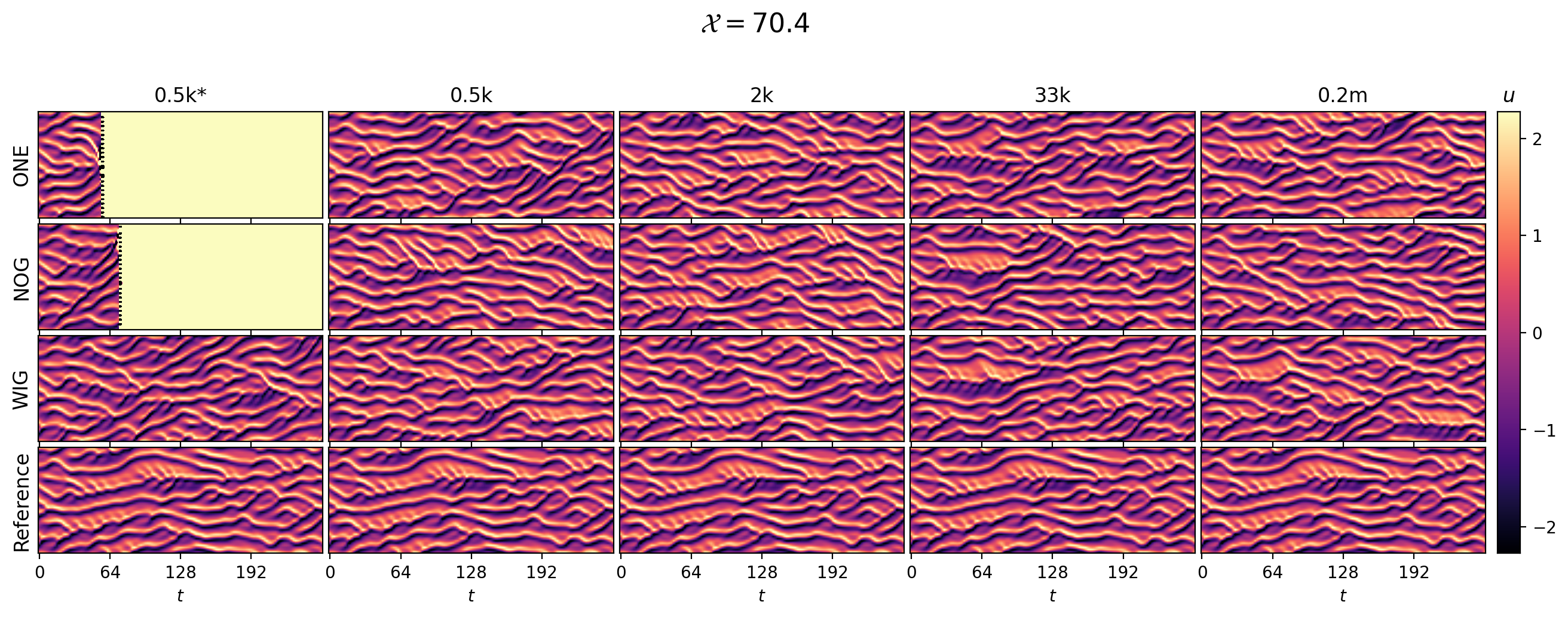
Figure 26: Inference error trajectory visualization of the GCN correction on the KS system for extrapolation on low $\mathcal{X}$

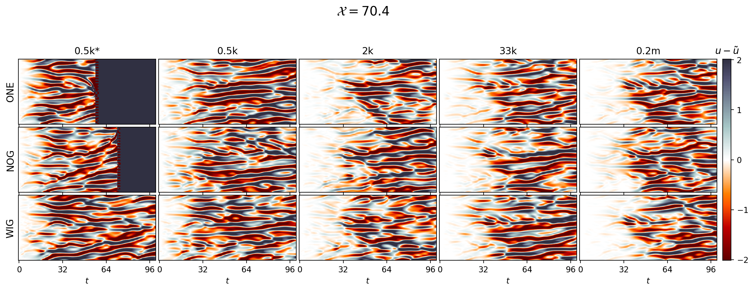
Figure 27: Inference error trajectory visualization of the GCN correction on the KS system for extrapolation on high $\mathcal{X}$

Figure 24 displays a sample inference trajectory for convolutional correction models trained with the three unrolling variants. The inference case is selected from the extrapolation dataset, in this case for the small domain size of $\mathcal{X}=30.2$, which lies outside of the training range. The difference to the reference is further visualized in figure 25. Here, the distance to the target state as $u-\tilde{u}$ is used. This error was evaluated for the full range of model sizes as introduced in section 4 and listed in table 2. The same visualization procedure was also done for the other extrapolation test on large domains with $\mathcal{X}=70.4$. Figures 26 and 27 similarly display the state trajectories and errors for a sample network. A clear trend of longer correlation horizons is visible in the error figures. As already expanded on in the main paper, larger architectures stay in proximity to the target evolution for longer inference rollouts. At the same time, unrolling reduces errors for a fixed size since NOG and WIG have smaller amplitudes. On the large domain sizes in figures 26 and 27, the networks also show instabilities when trained with ONE or NOG.

For the KOLM system, we visualize sample rollout trajectories for the extrapolation case of Re=1000 in figure 28. The displayed horizon spans 250 timesteps. The final step of this inference rollout is further visualized in figure 29 for the whole range of training setups, including unrolling variants and network sizes. Finally, a visualization of the solution error is provided in figure 30. The visualizations show how those networks that were trained with ONE and NOG unrolling tend to misinterpret points of high vorticity and generally produce larger errors. As pointed out in the main sections, network size is, along with training modality, a decisive contributor to inference accuracy. This observation can also be made in the error visualizations in 30.

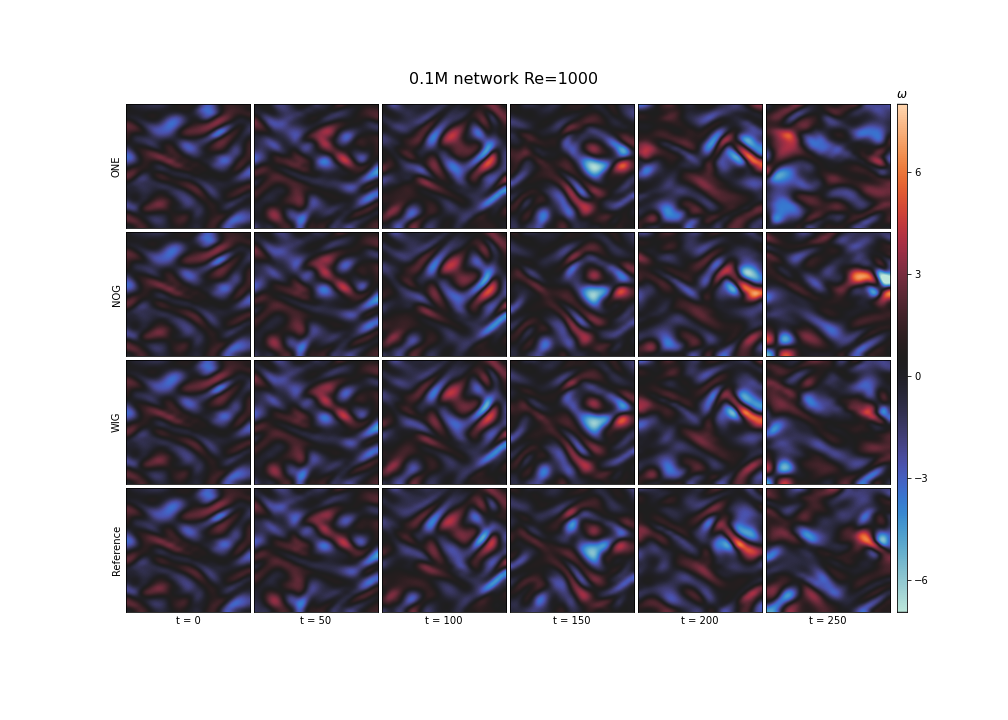
Figure 28: Inference vorticity after 250 steps of the CNN correction on the KOLM system for interpolation on intermediate Re=600, reference data is shown in the left column

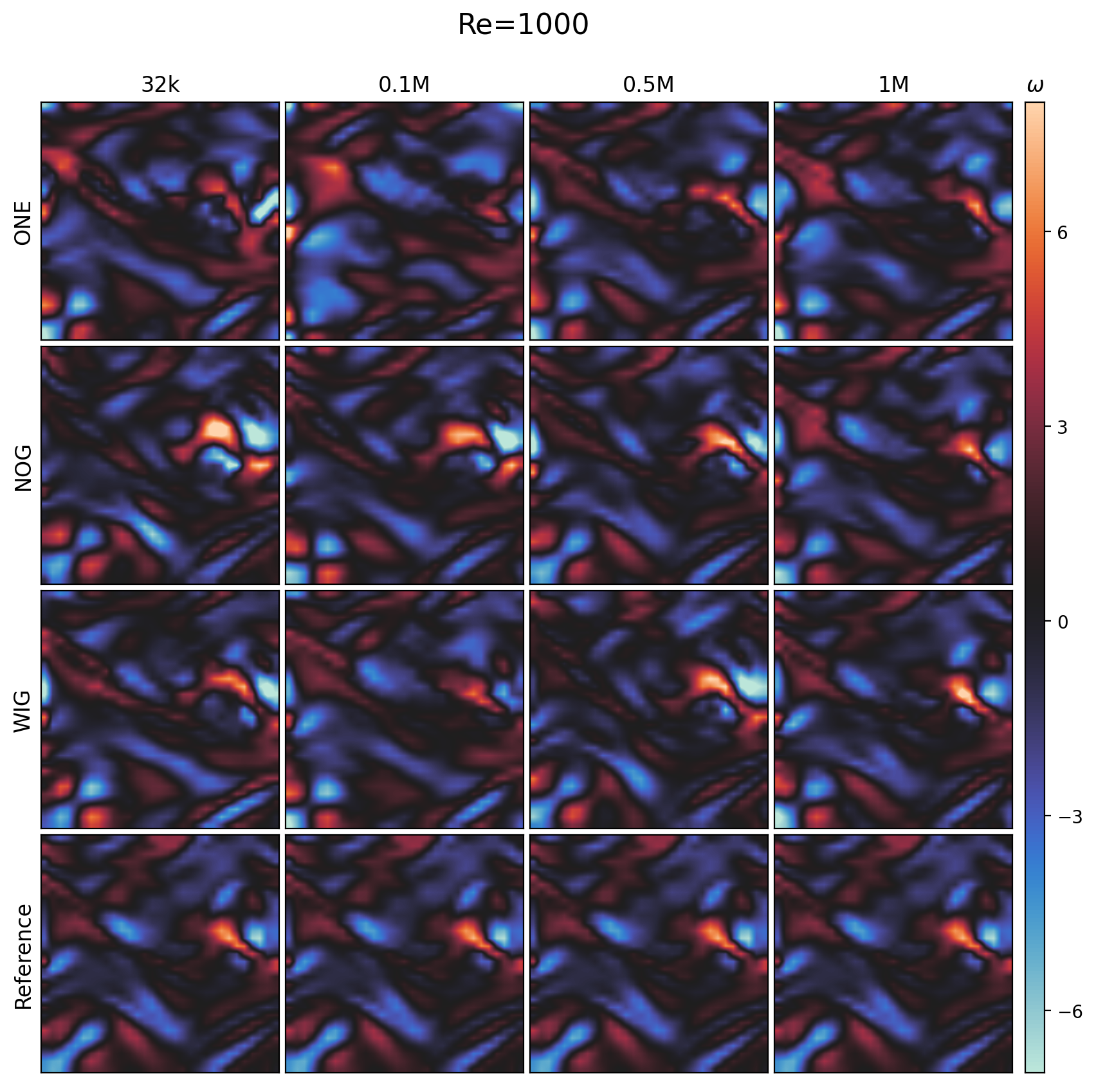
Figure 29: Inference vorticity after 250 steps of the CNN correction on the KOLM system for extrapolation on high Re=1000, reference data is shown in the left column

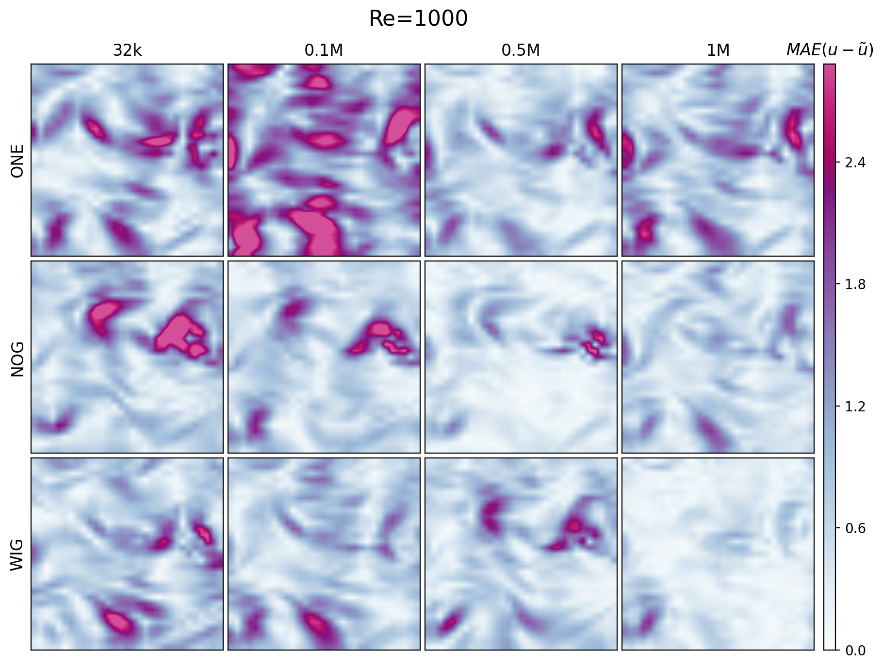
Figure 30: Inference vorticity after 250 steps of the CNN correction on the KOLM system for interpolation on intermediate Re=600, reference data is shown in the left column

Appendix E Evaluation Data

Herein, we provide the statistical data used to generate the figures in the main paper. The error data shown is always gathered from evaluations on a combined test set from interpolative and extrapolative cases, as described in appendix 4. For each initial frame in the test set, a trajectory is computed and errors with respect to the ground truth are accumulated, yielding one scalar error value per trajectory. Means and standard deviations are now calculated across these trajectories on a per-model-size and per-training-modality basis. Thus, the tables show these statistics for various model sizes, which are listed for the KS system in table 2, for the wake system in section 4.2, for the KOLM case in table 3, and for the AERO case in table 4. We denote the mean with an overline, e.g. as $\overline{\mathrm{ONE}}$, and the standard deviation as $\sigma$. Additionally, we perform a one-sided Welch’s t-test to the statistical significance of the empirical tests and their resulting distributions. For distributions with different means and standard deviations, [64] defines a t-test as

$$t=\frac{|\overline{X}_{1}-\overline{X}_{2}|}{\sqrt{\dfrac{\sigma_{1}^{2}}{M_{1}}+\dfrac{\sigma_{2}^{2}}{M_{2}}}}.$$ (21)

This holds for two distributions with mean $\overline{X}_{i}$, standard deviation $\sigma_{i}$, and sample sizes $M_{i}$. The p-value for a one-sided significance test is then computed as

$$p=Pr(T\leq t|H_{0}),$$ (22)

giving us the probability that the null-hypotheses (i.e. both distributions are identical) is true.

The differences in the studied training modalities are statistically significant for smaller network setups. As model sizes increase, the distribution of trained models becomes more similar. Our heavily overparameterized networks (e.g. 1.0M parameters for 48 degree of freedom KS system) all show highly accurate and stable predictions (see divergence time metric, Figure 20 Appendix C). Based on the theoretical considerations above, this means that the attractor of the learned dynamics is closely aligned with the ground truth system. These setups thus display less data shift and the benefits of unrolling are reduced. When these conditions in the overparameterized regime are met, NOG models are at a disadvantage due to their mismatch between gradients and loss landscape. However, these heavily oversized architectures are not practically relevant for scientific computing due to their weak scaling compared to numerical approaches. This evaluation confirms that for relevant, small to medium sized networks our results are statistically significant and hence that conclusions can be drawn.

The tables relate to the figures as follows:

• Figure 4 visualizes tables 5, 7, 8

• Figure 8 visualizes tables 14, 15, 16

• Figure 9 visualizes table 17

• Figure 11 visualizes tables 9, 10, 11

• Figure 13 visualizes tables 18, 19constant

• Figure 14 visualizes table 13

Table 5: Correction GCN $\mathcal{L}_{2}$ errors on the KS system

	$\overline{\mathrm{ONE}}$	$\overline{\mathrm{NOG}}$	$\overline{\mathrm{WIG}}$	$\sigma({\mathrm{ONE}})$	$\sigma({\mathrm{NOG}})$	$\sigma({\mathrm{WIG}})$	$p^{\mathrm{NOG}}_{\mathrm{ONE}}$	$p^{\mathrm{WIG}}_{\mathrm{ONE}}$
0.5k*	2.67063	2.07773	1.32860	0.61222	0.62611	0.09505	0.00220	0.00000
0.5k	3.42429	2.01830	1.15905	2.00918	0.81870	0.24652	0.00310	0.00001
2k	2.05080	1.53242	0.77671	1.58849	1.07397	0.20318	0.11706	0.00051
33k	0.42879	0.39406	0.33274	0.10139	0.11152	0.10516	0.15465	0.00278
0.2M	0.18810	0.20359	0.16093	0.04164	0.04815	0.05224	0.14164	0.03843
1M	0.12671	0.16176	0.12054	0.01942	0.03265	0.02622	0.00010	0.20174

Table 6: Correction CNN $\mathcal{L}_{2}$ errors on the KS system

	$\overline{\mathrm{ONE}}$	$\overline{\mathrm{NOG}}$	$\overline{\mathrm{WIG}}$	$\sigma({\mathrm{ONE}})$	$\sigma({\mathrm{NOG}})$	$\sigma({\mathrm{WIG}})$	$p^{\mathrm{NOG}}_{\mathrm{ONE}}$	$p^{\mathrm{WIG}}_{\mathrm{ONE}}$
0.5k*	2.79276	1.82674	1.36738	0.53627	0.33042	0.18318	0.00000	0.00000
0.5k	2.04899	1.77093	1.32922	0.76169	0.47778	0.46564	0.08736	0.00045
2k	1.04701	0.97612	0.80260	0.16266	0.10389	0.08582	0.05436	0.00000
33k	0.39871	0.42818	0.34545	0.08113	0.08503	0.05931	0.13464	0.01148
0.2M	0.23991	0.22823	0.19139	0.06584	0.05224	0.03468	0.26910	0.00296
1M	0.12554	0.16273	0.09885	0.01664	0.06723	0.01865	0.01067	0.00001
2M	0.09592	0.09519	0.07090	0.01241	0.01160	0.00889	0.42393	0.00000

Table 7: Correction CNN $\mathcal{L}_{2}$ errors on the WAKE system

	$\overline{\mathrm{ONE}}$	$\overline{\mathrm{NOG}}$	$\overline{\mathrm{WIG}}$	$\sigma({\mathrm{ONE}})$	$\sigma({\mathrm{NOG}})$	$\sigma({\mathrm{WIG}})$	$p^{\mathrm{NOG}}_{\mathrm{ONE}}$	$p^{\mathrm{WIG}}_{\mathrm{ONE}}$
6.3k	0.12045	0.07038	0.05515	0.02353	0.01374	0.00990	0.00001	0.00000
67k	0.07641	0.04430	0.03663	0.03321	0.01106	0.00568	0.00476	0.00076
1M	0.03389	0.02575	0.02496	0.00724	0.00733	0.00717	0.01120	0.00632

Table 8: Correction CNN $\mathcal{L}_{2}$ errors on the KOLM system

	$\overline{\mathrm{ONE}}$	$\overline{\mathrm{NOG}}$	$\overline{\mathrm{WIG}}$	$\sigma({\mathrm{ONE}})$	$\sigma({\mathrm{NOG}})$	$\sigma({\mathrm{WIG}})$	$p^{\mathrm{NOG}}_{\mathrm{ONE}}$	$p^{\mathrm{WIG}}_{\mathrm{ONE}}$
32k	0.04097	0.04140	0.03645	0.00833	0.00506	0.00398	0.45147	0.09404
0.1M	0.03064	0.02576	0.02504	0.00344	0.00511	0.00242	0.02090	0.00104
0.5Mk	0.01635	0.01394	0.01420	0.00172	0.00144	0.00201	0.00444	0.01878
1M	0.01046	0.00859	0.00820	0.00084	0.00110	0.00122	0.00093	0.00035

Table 9: Prediction GCN $\mathcal{L}_{2}$ errors on the KS system

	$\overline{\mathrm{ONE}}$	$\overline{\mathrm{NOG}}$	$\overline{\mathrm{WIG}}$	$\sigma({\mathrm{ONE}})$	$\sigma({\mathrm{NOG}})$	$\sigma({\mathrm{WIG}})$	$p^{\mathrm{NOG}}_{\mathrm{ONE}}$	$p^{\mathrm{WIG}}_{\mathrm{ONE}}$
0.5k*	7.98357	11.63567	10.23652	2.75299	1.57462	2.53653	0.00000	0.00526
0.5k	18.06462	5.10212	9.51381	5.02841	3.35803	4.80894	0.00000	0.00000
2k	10.41816	2.89637	5.62151	5.18653	0.92519	2.53810	0.00000	0.00033
33k	4.16912	1.44542	1.77320	2.10251	0.10168	0.68453	0.00000	0.00001
0.2M	1.13015	0.91450	0.79421	0.05839	0.08480	0.07173	0.00000	0.00000
1M	0.88423	0.81924	0.71090	0.05668	0.06682	0.07325	0.00101	0.00000

Table 10: Prediction CNN $\mathcal{L}_{2}$ errors on the KS system

	$\overline{\mathrm{ONE}}$	$\overline{\mathrm{NOG}}$	$\overline{\mathrm{WIG}}$	$\sigma({\mathrm{ONE}})$	$\sigma({\mathrm{NOG}})$	$\sigma({\mathrm{WIG}})$	$p^{\mathrm{NOG}}_{\mathrm{ONE}}$	$p^{\mathrm{WIG}}_{\mathrm{ONE}}$
0.5k*	19.87167	13.16589	17.09354	0.60110	2.18501	1.16960	0.00000	0.00000
0.5k	6.63006	4.37441	6.78108	3.99266	2.30527	2.03592	0.01744	0.44051
2k	2.51767	2.34324	2.73029	0.47555	0.34352	0.97282	0.09577	0.19269
33k	1.38413	1.49134	1.38093	0.18477	0.20430	0.15411	0.04493	0.47643
0.2M	1.02191	0.97444	0.87086	0.18962	0.12227	0.05520	0.17634	0.00075
1M	0.76798	0.85323	0.64513	0.06914	0.12842	0.04222	0.00638	0.00000

Table 11: Prediction CNN $\mathcal{L}_{2}$ errors on the WAKE system

	$\overline{\mathrm{ONE}}$	$\overline{\mathrm{NOG}}$	$\overline{\mathrm{WIG}}$	$\sigma({\mathrm{ONE}})$	$\sigma({\mathrm{NOG}})$	$\sigma({\mathrm{WIG}})$	$p^{\mathrm{NOG}}_{\mathrm{ONE}}$	$p^{\mathrm{WIG}}_{\mathrm{ONE}}$
6.3k	2307.82003	0.12045	0.11758	4614.57276	0.01364	0.01212	0.06560	0.06560
67k	0.15232	0.06248	0.06518	0.06279	0.00593	0.00545	0.00014	0.00018
1M	0.03336	0.03540	0.02791	0.00261	0.01500	0.00084	0.33794	0.00000

Table 12: Prediction CNN $\mathcal{L}_{2}$ errors on the KOLM system

	$\overline{\mathrm{ONE}}$	$\overline{\mathrm{NOG}}$	$\overline{\mathrm{WIG}}$	$\sigma({\mathrm{ONE}})$	$\sigma({\mathrm{NOG}})$	$\sigma({\mathrm{WIG}})$	$p^{\mathrm{NOG}}_{\mathrm{ONE}}$	$p^{\mathrm{WIG}}_{\mathrm{ONE}}$
32k	0.30455	0.27062	0.25849	0.09936	0.04430	0.03258	0.19624	0.11662
0.1M	0.11714	0.09850	0.10791	0.01839	0.00787	0.01187	0.00978	0.12649
0.5Mk	0.06879	0.06942	0.06790	0.01117	0.00656	0.00948	0.44579	0.43303
1M	0.04561	0.03582	0.03595	0.01311	0.00272	0.00856	0.02881	0.05153

Table 13: Prediction Unet $\mathcal{L}_{2}$ errors on the AERO system

	$\overline{\mathrm{ONE}}$	$\overline{\mathrm{NOG}}$	$\overline{\mathrm{WIG}}$	$\sigma({\mathrm{ONE}})$	$\sigma({\mathrm{NOG}})$	$\sigma({\mathrm{WIG}})$
0.5M	0.05046	0.03143	0.02975	0.01302	0.00420	0.00221
2M	0.03302	0.02815	0.02829	0.00251	0.00090	0.00106
8M	0.02892	0.02392	0.02388	0.00505	0.00153	0.00204

Table 14: Correction CNN $\mathcal{L}_{2}$ errors on KS system for multiple unrollings

	$\overline{\mathrm{NOG}}$	$\overline{\mathrm{WIG}}$	$\sigma({\mathrm{NOG}})$	$\sigma({\mathrm{WIG}})$
m=2	0.34026	0.33344	0.06799	0.07425
m=3	0.33358	0.32817	0.07953	0.05533
m=4	0.32845	0.31876	0.06794	0.05780
m=5	0.36300	0.29802	0.06534	0.06446
m=6	0.34506	0.29201	0.05682	0.06101
m=8	0.36041	0.28614	0.04762	0.04553
m=10	0.39730	0.28358	0.07861	0.06345
m=12	3.30768	0.26729	8.65391	0.07201
m=14	inf	0.25408	0.00000	0.06418
m=16	inf	0.24387	0.00000	0.05274
m=18	inf	0.25749	0.00000	0.05718
m=20	inf	3.46048	0.00000	9.12454

Table 15: Correction CNN $\mathcal{L}_{2}$ errors on KOLM system for multiple curriculums

	$\overline{\mathrm{NOG}}$	$\overline{\mathrm{WIG}}$	$\sigma({\mathrm{NOG}})$	$\sigma({\mathrm{WIG}})$
1-2-4	0.03064	0.01635	0.00344	0.00172
2-2-4	0.01046	0.04140	0.00084	0.00506
4-4-4	0.02576	0.01394	0.00511	0.00144

Table 16: Correction CNN $\mathcal{L}_{2}$ errors on KOLM system when trained without learning rate schedules

	$\overline{\mathrm{ONE}}$	$\overline{\mathrm{NOG}}$	$\overline{\mathrm{WIG}}$	$\sigma({\mathrm{ONE}})$	$\sigma({\mathrm{NOG}})$	$\sigma({\mathrm{WIG}})$
32k	0.04860	0.04563	0.05165	0.00651	0.00528	0.00626
0.1M	0.03478	0.03701	0.03708	0.00271	0.00689	0.00433
0.5M	0.03090	0.02827	0.03057	0.00267	0.00320	0.00332
1M	0.02935	0.02244	0.02635	0.00965	0.00398	0.00394

Table 17: Correction CNN $\mathcal{L}_{2}$ errors on KS system for gradient stopping variants

	m=6	m=6init	w=1	w=2	v=1	v=2
$\overline{\mathrm{WIG}}$	0.388526	0.281911	0.374733	0.396608	0.441374	0.407062
$\sigma({\mathrm{WIG}})$	0.092057	0.050417	0.097563	0.102014	0.156538	0.101093

Table 18: GCN $\mathcal{L}_{2}$ errors on KS system when transitioning from prediction to correction

	$\overline{\mathrm{ONE}}$	$\overline{\mathrm{NOG}}$	$\overline{\mathrm{WIG}}$	$\sigma({\mathrm{ONE}})$	$\sigma({\mathrm{NOG}})$	$\sigma({\mathrm{WIG}})$
10%	1.46963	1.15836	1.04210	0.27693	0.09666	0.15044
20%	1.22752	1.06870	0.92173	0.16561	0.11952	0.05283
30%	1.05448	1.13224	0.93338	0.17234	0.18949	0.10398
40%	0.98373	0.92035	0.77333	0.16078	0.12198	0.09403
50%	0.83278	0.78407	0.75527	0.11489	0.12352	0.11875
60%	0.73871	0.70152	0.61906	0.14414	0.09365	0.06889
70%	0.65280	0.61808	0.46474	0.10726	0.09699	0.07094
80%	0.46519	0.42852	0.39318	0.10353	0.10320	0.13866
90%	0.26651	0.15659	0.18686	0.09774	0.01506	0.06874

Table 19: CNN $\mathcal{L}_{2}$ errors on KS system when transitioning from prediction to correction

	$\overline{\mathrm{ONE}}$	$\overline{\mathrm{NOG}}$	$\overline{\mathrm{WIG}}$	$\sigma({\mathrm{ONE}})$	$\sigma({\mathrm{NOG}})$	$\sigma({\mathrm{WIG}})$
10%	1.08743	1.07423	1.00705	0.10005	0.08438	0.09433
20%	0.98619	0.97025	0.85021	0.12132	0.10936	0.07485
30%	0.89545	0.87275	0.82945	0.07255	0.10187	0.07454
40%	0.81295	0.81708	0.72305	0.13808	0.10260	0.06438
50%	0.70735	0.71738	0.66283	0.09532	0.08907	0.07525
60%	0.55892	0.60302	0.55926	0.12181	0.10013	0.05164
70%	0.45414	0.45675	0.48273	0.12301	0.11392	0.12604
80%	0.33173	0.28746	0.31830	0.08661	0.06363	0.07834
90%	0.14203	0.11449	0.12929	0.02205	0.01993	0.04566

References

- Abadi et al. [2016] M. Abadi et al. Tensorflow: A system for large-scale machine learning. In 12th USENIX symposium on operating systems design and implementation (OSDI 16), pages 265–283. USENIX Association, 2016.
- Bae and Koumoutsakos [2022] H. J. Bae and P. Koumoutsakos. Scientific multi-agent reinforcement learning for wall-models of turbulent flows. Nature Communications, 13(1):1443, 2022.
- Bar-Sinai et al. [2019] Yohai Bar-Sinai, Stephan Hoyer, Jason Hickey, and Michael P Brenner. Learning data-driven discretizations for partial differential equations. Proceedings of the National Academy of Sciences, 116(31):15344–15349, 2019.
- Beck and Kurz [2021] Andrea Beck and Marius Kurz. A perspective on machine learning methods in turbulence modeling. GAMM-Mitteilungen, 44(1):e202100002, 2021.
- Belkin [2021] Mikhail Belkin. Fit without fear: remarkable mathematical phenomena of deep learning through the prism of interpolation. Acta Numerica, 30:203–248, 2021.
- Bonnet et al. [2022] Florent Bonnet, Jocelyn Mazari, Paola Cinnella, and Patrick Gallinari. Airfrans: High fidelity computational fluid dynamics dataset for approximating reynolds-averaged navier–stokes solutions. Advances in Neural Information Processing Systems, 35:23463–23478, 2022.
- Brandstetter et al. [2022] Johannes Brandstetter, Daniel E. Worrall, and Max Welling. Message passing neural PDE solvers. In International Conference on Learning Representations, 2022.
- Bridson [2015] Robert Bridson. Fluid Simulation for Computer Graphics. CRC Press, 2015.
- Brunton et al. [2020] Steven L Brunton, Bernd R Noack, and Petros Koumoutsakos. Machine learning for fluid mechanics. Annual review of fluid mechanics, 52:477–508, 2020.
- Brunton et al. [2021] Steven L Brunton, Marko Budišić, Eurika Kaiser, and J Nathan Kutz. Modern koopman theory for dynamical systems. arXiv:2102.12086, 2021.
- Chung and Freund [2022] S. W. Chung and J. B. Freund. An optimization method for chaotic turbulent flow. Journal of Computational Physics, 457:111077, 2022.
- Cox and Matthews [2002] Steven M Cox and Paul C Matthews. Exponential time differencing for stiff systems. Journal of Computational Physics, 176(2):430–455, 2002.
- Duraisamy et al. [2019] Karthik Duraisamy, Gianluca Iaccarino, and Heng Xiao. Turbulence modeling in the age of data. Annual Review of Fluid Mechanics, 51:357–377, 2019.
- Eckert et al. [2019] Marie-Lena Eckert, Kiwon Um, and Nils Thuerey. Scalarflow: a large-scale volumetric data set of real-world scalar transport flows for computer animation and machine learning. ACM Transactions on Graphics (TOG), 38(6):1–16, 2019.
- Edson et al. [2019] Russell A Edson, Judith E Bunder, Trent W Mattner, and Anthony J Roberts. Lyapunov exponents of the kuramoto-sivashinsky pde. The ANZIAM Journal, 61(3):270–285, 2019. doi: 10.1017/S1446181119000105.
- Eivazi et al. [2021] Hamidreza Eivazi, Luca Guastoni, Philipp Schlatter, Hossein Azizpour, and Ricardo Vinuesa. Recurrent neural networks and koopman-based frameworks for temporal predictions in a low-order model of turbulence. International Journal of Heat and Fluid Flow, 90:108816, 2021. ISSN 0142-727X. doi: https://doi.org/10.1016/j.ijheatfluidflow.2021.108816.
- Ferziger et al. [2019] Joel H Ferziger, Milovan Perić, and Robert L Street. Computational methods for fluid dynamics. springer, 2019.
- Frank et al. [2020] Michael Frank, Dimitris Drikakis, and Vassilis Charissis. Machine-learning methods for computational science and engineering. Computation, 8(1):15, 2020.
- Geneva and Zabaras [2020] Nicholas Geneva and Nicholas Zabaras. Modeling the dynamics of pde systems with physics-constrained deep auto-regressive networks. Journal of Computational Physics, 403:109056, 2020.
- Geneva and Zabaras [2022] Nicholas Geneva and Nicholas Zabaras. Transformers for modeling physical systems. Neural Networks, 146:272–289, 2022. doi: 10.1016/j.neunet.2021.11.022.
- Givental et al. [2009] Alexander B. Givental, Boris A. Khesin, Jerrold E. Marsden, Alexander N. Varchenko, Victor A. Vassiliev, Oleg Ya. Viro, and Vladimir M. Zakalyukin, editors. Kolmogorov seminar on selected questions of analysis, pages 144–148. Springer, 2009. doi: 10.1007/978-3-642-01742-1˙8.
- Han et al. [2021] Xu Han, Han Gao, Tobias Pfaff, Jian-Xun Wang, and Liping Liu. Predicting physics in mesh-reduced space with temporal attention. In International Conference on Learning Representations, 2021.
- He et al. [2016] Kaiming He, Xiangyu Zhang, Shaoqing Ren, and Jian Sun. Deep residual learning for image recognition. In Proceedings of the IEEE conference on computer vision and pattern recognition, pages 770–778, 2016.
- Holl et al. [2020] Philipp Holl, Vladlen Koltun, Kiwon Um, and Nils Thuerey. phiflow: A differentiable pde solving framework for deep learning via physical simulations. In NeurIPS workshop, volume 2, 2020.
- Hu et al. [2019] Yuanming Hu, Luke Anderson, Tzu-Mao Li, Qi Sun, Nathan Carr, Jonathan Ragan-Kelley, and Frédo Durand. Difftaichi: Differentiable programming for physical simulation. arXiv:1910.00935, 2019.
- Issa [1986] Raad I Issa. Solution of the implicitly discretised fluid flow equations by operator-splitting. Journal of computational physics, 62(1):40–65, 1986.
- Janny et al. [2023] Steeven Janny, Aurélien Beneteau, Nicolas Thome, Madiha Nadri, Julie Digne, and Christian Wolf. Eagle: Large-scale learning of turbulent fluid dynamics with mesh transformers. In International Conference on Learning Representations, 2023.
- Kochkov et al. [2021] Dmitrii Kochkov, Jamie A Smith, Ayya Alieva, Qing Wang, Michael P Brenner, and Stephan Hoyer. Machine learning–accelerated computational fluid dynamics. Proceedings of the National Academy of Sciences, 118(21):e2101784118, 2021.
- Kohl et al. [2023] Georg Kohl, Li-Wei Chen, and Nils Thuerey. Turbulent flow simulation using autoregressive conditional diffusion models. arXiv:2309.01745, 2023.
- Lam et al. [2022] Remi Lam, Alvaro Sanchez-Gonzalez, Matthew Willson, Peter Wirnsberger, Meire Fortunato, Alexander Pritzel, Suman Ravuri, Timo Ewalds, Ferran Alet, Zach Eaton-Rosen, et al. Graphcast: Learning skillful medium-range global weather forecasting. arXiv:2212.12794, 2022.
- Li et al. [2019] Guohao Li, Matthias Muller, Ali Thabet, and Bernard Ghanem. Deepgcns: Can gcns go as deep as cnns? In Proceedings of the IEEE/CVF international conference on computer vision, pages 9267–9276, 2019.
- Li et al. [2022] Zijie Li, Kazem Meidani, and Amir Barati Farimani. Transformer for partial differential equations’ operator learning. arXiv:2205.13671, 2022.
- Li et al. [2020] Zongyi Li, Nikola Kovachki, Kamyar Azizzadenesheli, Burigede Liu, Kaushik Bhattacharya, Andrew Stuart, and Anima Anandkumar. Fourier neural operator for parametric partial differential equations. arXiv:2010.08895, 2020.
- Lienen et al. [2023] Marten Lienen, Jan Hansen-Palmus, David Lüdke, and Stephan Günnemann. Generative diffusion for 3d turbulent flows. arXiv:2306.01776, 2023.
- Ling et al. [2016] J. Ling, A. Kurzawski, and J. Templeton. Reynolds averaged turbulence modelling using deep neural networks with embedded invariance. Journal of Fluid Mechanics, 807:155–166, 2016.
- Lippe et al. [2023] Phillip Lippe, Bastiaan S Veeling, Paris Perdikaris, Richard E Turner, and Johannes Brandstetter. Pde-refiner: Achieving accurate long rollouts with neural pde solvers. arXiv:2308.05732, 2023.
- List et al. [2022] Björn List, Li-Wei Chen, and Nils Thuerey. Learned turbulence modelling with differentiable fluid solvers: physics-based loss functions and optimisation horizons. Journal of Fluid Mechanics, 949:A25, 2022. doi: 10.1017/jfm.2022.738.
- Lusch et al. [2018] Bethany Lusch, J Nathan Kutz, and Steven L Brunton. Deep learning for universal linear embeddings of nonlinear dynamics. Nature communications, 9(1):1–10, 2018.
- MacArt et al. [2021] Jonathan F MacArt, Justin Sirignano, and Jonathan B Freund. Embedded training of neural-network subgrid-scale turbulence models. Physical Review Fluids, 6(5):050502, 2021.
- Margazoglou and Magri [2023] G. Margazoglou and L. Magri. Stability analysis of chaotic systems from data. Nonlinear Dynamics, 111(9):8799–8819, 2023.
- Melchers et al. [2023] Hugo Melchers, Daan Crommelin, Barry Koren, Vlado Menkovski, and Benjamin Sanderse. Comparison of neural closure models for discretised pdes. Computers & Mathematics with Applications, 143:94–107, 2023.
- Mikhaeil et al. [2022] Jonas Mikhaeil, Zahra Monfared, and Daniel Durstewitz. On the difficulty of learning chaotic dynamics with RNNs. Advances in Neural Information Processing Systems, 35:11297–11312, 2022.
- Novati et al. [2021] G. Novati, H. L. de Laroussilhe, and P. Koumoutsakos. Automating turbulence modelling by multi-agent reinforcement learning. Nature Machine Intelligence, 3(1):87–96, 2021.
- Oktay et al. [2018] Ozan Oktay, Jo Schlemper, Loic Le Folgoc, Matthew Lee, Mattias Heinrich, Kazunari Misawa, Kensaku Mori, Steven McDonagh, Nils Y Hammerla, Bernhard Kainz, et al. Attention u-net: Learning where to look for the pancreas. arXiv:1804.03999, 2018.
- Paszke et al. [2019] Adam Paszke, Sam Gross, Francisco Massa, Adam Lerer, James Bradbury, Gregory Chanan, Trevor Killeen, Zeming Lin, Natalia Gimelshein, Luca Antiga, Alban Desmaison, Andreas Kopf, Edward Yang, Zachary DeVito, Martin Raison, Alykhan Tejani, Sasank Chilamkurthy, Benoit Steiner, Lu Fang, Junjie Bai, and Soumith Chintala. Pytorch: An imperative style, high-performance deep learning library. In Advances in Neural Information Processing Systems 32, pages 8024–8035. Curran Associates, Inc., 2019. URL http://papers.neurips.cc/paper/9015-pytorch-an-imperative-style-high-performance-deep-learning-library.pdf.
- Pfaff et al. [2020] Tobias Pfaff, Meire Fortunato, Alvaro Sanchez-Gonzalez, and Peter W Battaglia. Learning mesh-based simulation with graph networks. arXiv:2010.03409, 2020.
- Prantl et al. [2022] Lukas Prantl, Benjamin Ummenhofer, Vladlen Koltun, and Nils Thuerey. Guaranteed conservation of momentum for learning particle-based fluid dynamics. Advances in Neural Information Processing Systems, 35, 2022.
- Raissi et al. [2019] Maziar Raissi, Paris Perdikaris, and George E Karniadakis. Physics-informed neural networks: A deep learning framework for solving forward and inverse problems involving nonlinear partial differential equations. Journal of Computational physics, 378:686–707, 2019.
- Rumsey [2010] Christopher L Rumsey. CFL3D contribution to the AIAA supersonic shock boundary layer interaction workshop. NASA TM–2010-216858, 2010.
- Rumsey et al. [1997] Christopher Lockwood Rumsey, Robert T Biedron, and James Lee Thomas. CFL3D: its history and some recent applications. NASA TM–112861, 1997.
- Sanchez-Gonzalez et al. [2020] Alvaro Sanchez-Gonzalez, Jonathan Godwin, Tobias Pfaff, Rex Ying, Jure Leskovec, and Peter Battaglia. Learning to simulate complex physics with graph networks. In Proceedings of the 37th International Conference on Machine Learning, volume 119 of Proceedings of Machine Learning Research, pages 8459–8468. PMLR, 2020.
- Sirignano et al. [2020] Justin Sirignano, Jonathan F MacArt, and Jonathan B Freund. Dpm: A deep learning pde augmentation method with application to large-eddy simulation. Journal of Computational Physics, 423:109811, 2020. ISSN 0021-9991.
- Stachenfeld et al. [2021] Kimberly Stachenfeld, Drummond B Fielding, Dmitrii Kochkov, Miles Cranmer, Tobias Pfaff, Jonathan Godwin, Can Cui, Shirley Ho, Peter Battaglia, and Alvaro Sanchez-Gonzalez. Learned coarse models for efficient turbulence simulation. arXiv:2112.15275, 2021.
- Suh et al. [2022] Hyung Ju Suh, Max Simchowitz, Kaiqing Zhang, and Russ Tedrake. Do differentiable simulators give better policy gradients? In International Conference on Machine Learning, volume 162 of Proceedings of Machine Learning Research, pages 20668–20696. PMLR, 17–23 Jul 2022.
- Sutskever [2013] Ilya Sutskever. Training recurrent neural networks. University of Toronto Toronto, ON, Canada, 2013.
- Um et al. [2020] Kiwon Um, Robert Brand, Yun Raymond Fei, Philipp Holl, and Nils Thuerey. Solver-in-the-loop: Learning from differentiable physics to interact with iterative pde-solvers. In Advances in Neural Information Processing Systems, pages 6111–6122. Curran Associates, Inc., 2020.
- Ummenhofer et al. [2019] Benjamin Ummenhofer, Lukas Prantl, Nils Thuerey, and Vladlen Koltun. Lagrangian fluid simulation with continuous convolutions. In International Conference on Learning Representations, 2019.
- van Gastelen et al. [2023] T. van Gastelen, W. Edeling, and B. Sanderse. Energy-conserving neural network for turbulence closure modeling. arXiv preprint arXiv:2301.13770, 2023.
- Vlachas et al. [2022] P. R. Vlachas, G. Arampatzis, C. Uhler, and P. Koumoutsakos. Multiscale simulations of complex systems by learning their effective dynamics. Nature Machine Intelligence, 4(4):359–366, 2022.
- von Rueden et al. [2020] Laura von Rueden, Sebastian Mayer, Rafet Sifa, Christian Bauckhage, and Jochen Garcke. Combining machine learning and simulation to a hybrid modelling approach: Current and future directions. In International Symposium on Intelligent Data Analysis, pages 548–560. Springer, 2020.
- Wang et al. [2020] Rui Wang, Karthik Kashinath, Mustafa Mustafa, Adrian Albert, and Rose Yu. Towards physics-informed deep learning for turbulent flow prediction. In Proceedings of the 26th ACM SIGKDD International Conference on Knowledge Discovery & Data Mining, pages 1457–1466, 2020.
- Wang et al. [2022] Rui Wang, Yihe Dong, Sercan O Arik, and Rose Yu. Koopman neural forecaster for time series with temporal distribution shifts. arXiv:2210.03675, 2022.
- Wang et al. [2019] Yue Wang, Yongbin Sun, Ziwei Liu, Sanjay E Sarma, Michael M Bronstein, and Justin M Solomon. Dynamic graph cnn for learning on point clouds. ACM Transactions on Graphics (tog), 38(5):1–12, 2019.
- Welch [1947] B. L. Welch. The generalization of ‘student’s’ problem when several different population variances are involved. Biometrika, 34(1-2):28–35, 1947.
- Wiewel et al. [2019] Steffen Wiewel, Moritz Becher, and Nils Thuerey. Latent space physics: Towards learning the temporal evolution of fluid flow. In Computer graphics forum, volume 38(2), pages 71–82. Wiley Online Library, 2019.
- Wiles et al. [2021] Olivia Wiles, Sven Gowal, Florian Stimberg, Sylvestre Alvise-Rebuffi, Ira Ktena, Krishnamurthy Dvijotham, and Taylan Cemgil. A fine-grained analysis on distribution shift. arXiv:2110.11328, 2021.
- Wu et al. [2020] Jin-Long Wu, Karthik Kashinath, Adrian Albert, Dragos Chirila, Heng Xiao, et al. Enforcing statistical constraints in generative adversarial networks for modeling chaotic dynamical systems. Journal of Computational Physics, 406:109209, 2020.
- Wu et al. [2022] Tailin Wu, Takashi Maruyama, and Jure Leskovec. Learning to accelerate partial differential equations via latent global evolution. Advances in Neural Information Processing Systems, 35:2240–2253, 2022.
- Xian et al. [2022] Zhou Xian, Bo Zhu, Zhenjia Xu, Hsiao-Yu Tung, Antonio Torralba, Katerina Fragkiadaki, and Chuang Gan. Fluidlab: A differentiable environment for benchmarking complex fluid manipulation. In International Conference on Learning Representations, 2022.
- Yang et al. [2021] Liu Yang, Xuhui Meng, and George Em Karniadakis. B-pinns: Bayesian physics-informed neural networks for forward and inverse pde problems with noisy data. Journal of Computational Physics, 425:109913, 2021.
- Zhang et al. [2022] X.-L. Zhang, H. Xiao, X. Luo, and G. He. Ensemble kalman method for learning turbulence models from indirect observation data. Journal of Fluid Mechanics, 949:A26, 2022.
- Zhang et al. [2023] X.-L. Zhang, H. Xiao, X. Luo, and G. He. Combining direct and indirect sparse data for learning generalizable turbulence models. Journal of Computational Physics, page 112272, 2023.