Compact sum-of-products form of the molecular electronic Hamiltonian based on canonical polyadic decomposition

Abstract

We propose an approach to represent the second-quantized electronic Hamiltonian in a compact sum-of-products (SOP) form. The approach is based on the canonical polyadic decomposition (CPD) of the original Hamiltonian projected onto the sub-Fock spaces formed by groups of spin orbitals. The algorithm for obtaining the canonical polyadic form starts from an exact sum-of-products, which is then optimally compactified using an alternating least-squares procedure. We discuss the relation of this specific SOP with related forms, namely the Tucker format and the matrix product operator often used in conjunction with matrix product states. We benchmark the method on the electronic dynamics of an excited water molecule, trans-polyenes, and the charge migration in glycine upon inner-valence ionization. The quantum dynamics are performed with the multilayer multi-configuration time-dependent Hartree method in second quantization representation (MCTDH-SQR). Other methods based on tree-tensor Ansätze may profit from this general approach.

I Introduction

The multiconfiguration time-dependent Hartree (MCTDH)  [1, 2, 3, 4, 5] and its multilayer generalization (ML-MCTDH)  [6, 7, 8, 9, 10] are highly efficient methods for simulating the quantum dynamics of nuclear degrees of freedom in high-dimensional systems. In its original form, the MCTDH Ansatz cannot describe systems of indistinguishable particles, as it assumes a product form of the underlying single particle functions (SPFs), thereby failing to account for the proper symmetry of these indistinguishable particles. However, it is possible to construct the multiconfiguration wavefunction using Slater determinants and permanents as the basis to address fermionic and bosonic systems, respectively. These specialized theories are referred to as MCTDH for fermions (MCTDH-F)  [11, 12, 13, 14, 15] and bosons (MCTDH-B) [12, 16]. A unified version of the two theories has been established, employing a non-symmetric core tensor to connect mixtures of different types of indistinguishable particles [17]. However, a limitation of such descriptions arises from the combinatorial increase in the number of configurations within the electronic/bosonic subsystem as the number of particles and single-particle functions grows. Additionally, the requirement of antisymmetry or symmetry hinders their further decomposition into smaller-rank tensors. Consequently, when dealing with the same type of indistinguishable particles, both the MCTDH-B and MCTDH-F approaches are incompatible with the multilayer extension of the MCTDH framework.

A fundamentally different approach for describing systems of indistinguishable particles is the use of the second quantization representation. Wang and Thoss introduced and applied this approach within the context of MCTDH, naming it MCTDH in SQR (MCTDH-SQR) [18]. In this representation, the state of the system is described using the occupation number representation, which corresponds to the occupation of specific sets of spin-orbitals. The symmetry of the indistinguishable particles is expressed through the creation and annihilation operators that operate on the system’s state. Since the occupation of individual spin-orbitals is treated as analogous to a coordinate in the traditional MCTDH formulation, the degrees of freedom (DOFs) become distinguishable, making it straightforward to construct a multilayer Ansatz for the wavefunction.

The MCTDH-SQR method has found applications in various domains after its introduction, including solving the impurity problem in non-equilibrium dynamical mean-field theory [19] and addressing quantum transport in molecular junctions [20, 21, 22] and quantum dots [23, 24]. Additionally, Manthe and Weike developed an MCTDH-SQR approach based on time-dependent optimal orbitals, known as the MCTDH-oSQR method [25, 26]. These applications primarily dealt with model Hamiltonians  [18, 19, 25, 26, 20, 21, 22, 23, 24]. More recently, we extended the MCTDH-SQR method to describe non-adiabatic dynamics in molecular systems. This extension is based on the second-quantized representation of the electrons and the first-quantized representation of the nuclear coordinates, while also providing expressions for the non-adiabatic coupling matrix elements within this combined representation [27]. In this formalism, the non-adiabatic effects are considered within the time-evolving electronic subsystem coupled with the dynamics of the nuclei, thus bypassing the explicit determination of potential energy surfaces and non-adiabatic couplings and offering an alternative to the conventional group Born-Oppenheimer (BO) approximation.

Nonetheless, a significant challenge remains when applying the MCTDH-SQR method to ab initio studies of large molecular systems, namely the unfavourable scaling of the number of terms in the electronic SQR Hamiltonian, which increases with the fourth power of the number of spin-orbitals. The density matrix renormalization group (DMRG) [28, 29, 30] formalism, which shares a tensor representation framework similar to ML-MCTDH, mitigates this scaling by representing the Hamiltonian as a matrix product operator (MPO) [31, 32, 33, 34, 35, 36], compatible with the matrix product state (MPS) [31, 33] structure of the wavefunction. In contrast, a comparably concise representation of the electronic Hamiltonian compatible with the sum-of-products (SOP)–based MCTDH algorithm is not yet available. In the SOP form, a high-dimensional operator is represented as a sum of products of operators. Every operator in each product acts within the space of the corresponding primitive (or physical) degree of freedom.

When treating high-dimensional nuclear dynamics problems, obtaining such a SOP representation of the operator is a major challenge: while the kinetic energy operator is often in this form, this is not true for the potential energy surface. A wide range of methods have therefore been developed to transform general potential energy surfaces into SOP format. These methods encompass approaches such as POTFIT [3, 37, 38], multigrid POTFIT [39], Monte Carlo POTFIT [40], as well as the multilayer extension of POTFIT [41, 42], and Monte Carlo canonical polyadic decomposition (MCCPD) [43]. Additionally, some algorithms utilize neural network techniques [44, 45, 46, 47, 48, 49, 50]. Note also that there are alternative MCTDH implementations that do not require the SOP form of the operator - for example, the correlation discrete variable representation of Manthe [51] and the collocation-MCTDH method of Wodraszka and Carrington [52].

Recently, we introduced an approach based on the Tucker decomposition, hence similar to POTFIT, to represent a compact SOP form of the second quantized electronic Hamiltonian, where the term compact refers to a smaller number of SOP terms compared to the original SQR Hamiltonian [53]. Unfortunately, this approach suffers from a poor scaling due to the presence of a core tensor acting on a direct product of operator subspaces. In the present work, we introduce and benchmark an approach based on canonical polyadic decomposition (CPD), which serves two purposes: first, it mitigates the quartic scaling of the electronic Hamiltonian with respect to the number of spin-orbitals. Second, compared to the Tucker format, CPD does not feature a core tensor of expansion coefficients on top of an orthogonal basis of one-particle operators. Instead, the products of the expansion are independent of each other offering, potentially, a much more favourable scaling. As we discuss below, the MPO form often used in DMRG lies conceptually in between two limiting cases: the Tucker format and CPD.

The paper is organized as follows. Section II.1 discusses the general strategy to write the SQR electronic Hamiltonian in SOP form. Section II.2 reviews the choice of DOF in the MCTDH-SQR formalism. Section II.3 introduces strategies that lead to compact SOP forms of the electronic SQR Hamiltonian, in particular CPD, and its connection to the MPO form. Secs III.1 and  III.2 and  III.3 present and discuss numerical results on H₂O, trans-C₈H₁₀, and glycine, respectively. The scaling of various coefficients related to the ML-MCTDH-SQR method is briefly discussed in Section IV. Finally, a summary and conclusions are provided in Section V.

II Theory

II.1 Sum-of-products form of the electronic Hamiltonian

The ab initio electronic Hamiltonian in the second quantization framework reads

$$\hat{H}=\sum_{ij}h_{ij}\hat{a}_{i}^{\dagger}\hat{a}_{j}+\frac{1}{2}\sum_{ijkl}v_{ijkl}\hat{a}_{i}^{\dagger}\hat{a}_{j}^{\dagger}\hat{a}_{l}\hat{a}_{k},$$ (1)

where

$$h_{ij}=\langle\phi_{i}(1)|-\frac{1}{2}\nabla_{1}^{2}-\sum_{A=1}^{M}\frac{Z_{A}}{r_{{}_{1A}}}|\phi_{j}(1)\rangle,$$ (2)

$$v_{ijkl}=\langle\phi_{i}(1)\phi_{j}(2)|\frac{1}{r_{12}}|\phi_{k}(1)\phi_{l}(2)\rangle,$$ (3)

are the one- and two-body integrals, involving the spin orbitals $\phi_{i}$, respectively. The $\hat{a}_{i}$ and $\hat{a}_{i}^{\dagger}$ correspond to the annihilation and creation operators that annihilate and create an electron in the $i$-th spin orbitals, respectively, satisfy the fermionic commutation relations

$$\{\hat{a}_{i},\hat{a}_{j}^{\dagger}\}=\hat{a}_{i}\hat{a}_{j}^{\dagger}+\hat{a}_{j}^{\dagger}\hat{a}_{i}=\delta_{ij},$$ (4)

$$\{\hat{a}_{i}^{\dagger},\hat{a}_{j}^{\dagger}\}=\{\hat{a}_{i},\hat{a}_{j}\}=0.$$ (5)

Although the electronic Hamiltonian in Eq. 1 seems like already being in a SOP form, the anti-commutation relations of the fermionic creation and annihilation operators in Eqs. 4 and 5 lead to the accumulation of a phase factor $S_{s}=\sum_{k=1}^{s-1}n_{k}$ depending on the occupation of all spin-orbitals before the $s$-th position for $\hat{a}_{s}^{\dagger}$ acting on a Fock-space configuration (the same is true for $\hat{a}_{s}$) [54]

$$\hat{a}_{s}^{\dagger}|n_{1},n_{2},\dots,n_{M}\rangle=\hat{a}_{s}^{\dagger}(\hat{a}_{1}^{\dagger})^{n_{1}}(\hat{a}_{2}^{\dagger})^{n_{2}}\cdots(\hat{a}_{M}^{\dagger})^{n_{M}}|\mathrm{0}\rangle$$

$$=(-1)^{S_{s}}(\hat{a}_{1}^{\dagger})^{n_{1}}(\hat{a}_{2}^{\dagger})^{n_{2}}\cdots[\hat{a}_{s}^{\dagger}(\hat{a}_{s}^{\dagger})^{n_{s}}]\cdots(\hat{a}_{M}^{\dagger})^{n_{M}}|\mathrm{0}\rangle.$$ (6)

This phase factor makes the creation and annihilation operator nonlocal, i.e., the operator $\hat{a}_{s}^{(\dagger)}$ acts beyond its index $s$ and therefore the electronic SQR Hamiltonian is, in general, not in the SOP form with respect to the primitive degrees of freedom. Wang and Thoss resolved this issue by mapping the fermionic operators onto equivalent spin operators [18]. Formally, this mapping consists of applying the inverse Jordan-Wigner (JW) transformation to the fermionic field operators and effectively transforming the fermionic Hamiltonian into an equivalent spin-chain Hamiltonian [55]. The equivalent spin-$1/2$ chain Hamiltonian after the JW transformation reads [27]

$$\hat{H}= \sum_{ij}h_{{}_{ij}}\left(\prod_{q=a+1}^{b-1}\hat{\sigma}^{z}_{q}\right)\hat{\sigma}_{i}^{+}\hat{\sigma}_{j}^{-}$$

$$+ \frac{1}{2}\sum_{ijkl}v_{{}_{ijkl}}\left(\prod_{q=a+1}^{b-1}\hat{\sigma}^{z}_{q}\prod_{q^{\prime}=c+1}^{d-1}\hat{\sigma}^{z}_{q^{\prime}}\right)$$

$$\mathrm{sgn}(j-i)\mathrm{sgn}(l-k)\hat{\sigma}_{i}^{+}\hat{\sigma}_{j}^{+}\hat{\sigma}_{l}^{-}\hat{\sigma}_{k}^{-}.$$ (7)

where $\hat{\sigma}_{i}^{+}=\frac{1}{2}\left(\hat{\sigma}_{i}^{x}+i\hat{\sigma}_{i}^{y}\right)$, $\hat{\sigma}_{i}^{-}=\frac{1}{2}\left(\hat{\sigma}_{i}^{x}-i\hat{\sigma}_{i}^{y}\right)$, and $\hat{\sigma}_{k}^{z}$ are the standard spin ladder operators with Pauli matrices $\bm{\sigma}^{x}$, $\bm{\sigma}^{y}$ and $\bm{\sigma}^{z}$. Here the indices $(a,b,c,d)$ correspond to the $(i,j,k,l)$ indices, but ordered from smaller to larger and the $\mathrm{sgn}$ function is defined as

$$\mathrm{sgn}(x)=\begin{cases}1,&\text{if }x\geq 0\\ -1,&\text{otherwise}.\end{cases}$$ (8)

The operators $\hat{\sigma}_{\kappa}^{+}$, $\hat{\sigma}_{\kappa}^{-}$ and $\hat{\sigma}^{z}_{\kappa}$ act now locally on $\kappa$-th spin-$\frac{1}{2}$ basis function and their matrix representation reads

$$\bm{\sigma}^{+}=\begin{pmatrix}0&0\\ 1&0\\ \end{pmatrix};\,\,\,\,\bm{\sigma^{-}}=\begin{pmatrix}0&1\\ 0&0\\ \end{pmatrix};\,\,\,\,\bm{\sigma^{z}}=\begin{pmatrix}1&0\\ 0&-1\\ \end{pmatrix}.$$ (9)

Clearly, the electronic Hamiltonian written in Eq. II.1 is in the SOP form with respect to the primitive DOFs (spin-$\frac{1}{2}$ basis).

II.2 Spin and Fock space degree of freedom

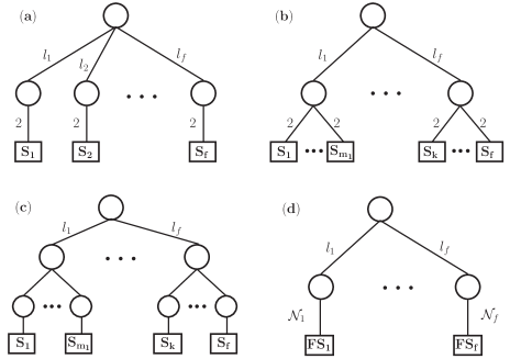
Figure 1: Tree structures for the various MCTDH-SQR wavefunction Ansätze: (a) Normal MCTDH wavefunction tree, in which the spin degree of freedoms (S-DOF) are considered as primitive DOFs. (b) MCTDH wavefunction tree with mode combination, in which S-DOFs are considered as primitive DOFs. (c) ML-MCTDH wavefunction tree, in which S-DOFs are considered as primitive DOFs. (d) MCTDH wavefunction tree, in which the Fock space of a group of spin orbitals is considered as single DOF (FS-DOF). $l_{\kappa}$ denotes number of SPF of the $\kappa$-th mode and $\mathcal{N}_{\kappa}$ is the number of configuration of $\kappa$-th FS-DOF.

In the above formulation there are two limiting MCTDH-SQR wavefunction Ansätze: Each spin degree of freedom (S-DOF) is described by either (i) one or (ii) two time-dependent SPFs. The former corresponds to a time-dependent Hartree (TDH) wavefunction with a single Hartree product and the latter corresponds to the exact wavefunction consisting of 2^M configurations, where M is the number of S-DOF. Thus, the limiting case (i) leads to a poor description of a correlated state and the latter leads to an exact formulation, which becomes quickly unaffordable as the number of S-DOF (i.e., spin orbitals) increases. Therefore, the only practical way to apply the MCTDH-SQR method is to create groups of S-DOFs, either through mode combination or through its multi-layer generalization (ML-MCTDH). Figures 1 (a), (b), and (c) show the normal MCTDH wavefunction, MCTDH wavefunction with mode combination, and ML-MCTDH wavefunction, respectively, where S-DOFs are used as primitive DOFs.

For $M$ spin orbitals there are 2^M Fock states. On the other hand, one can divide the total Fock space into $f$ sub-Fock spaces by grouping the M spin orbitals into $f$ groups ($m_{1}$, $m_{2}$, $\cdots$, $m_{f}$)

$$\mathcal{F}(M)=\mathcal{F}_{1}(m_{1})\otimes\mathcal{F}_{2}(m_{2})\otimes\dots\otimes\mathcal{F}_{f}(m_{f})$$ (10)

where $\mathcal{F}_{\kappa}(m_{\kappa})$ denotes the sub-Fock space of the $\kappa$-th FS-DOF (consists of $m_{\kappa}$ S-DOFs) with $\mathcal{N}_{\kappa}$ (=2${}^{m_{\kappa}}$) Fock states and

$$M=\sum_{\kappa=1}^{f}m_{\kappa}.$$ (11)

Now, one can represent the configurations of the sub-Fock space $\mathcal{F}_{\kappa}(m_{\kappa})$ as a new primitive DOF. We refer to this representation of the primitive DOF as Fock space DOF (FS-DOF). Fig. 1 (d) shows the MCTDH wavefunction involving FS-DOF as primitive DOF. In the FS-DOF formalism, one needs to transform the primitive operator string described in the Eq. II.1 into new primitive matrix operators acting onto the sub-Fock spaces of their corresponding FS-DOF.

In the FS-DOF representation, the state of the system is described by kets $|i_{1},\ldots,i_{f}\rangle$, where $i_{\kappa}$ corresponds to the $i$-th configuration of the $\kappa$-th FS-DOF. One can think of the $i_{\kappa}$ configuration indices as indexing Euclidean basis vectors within each degree of freedom. The configurations within a FS-DOF can correspond, in general, to different electron occupation numbers. A matrix element of the total Hamiltonian is then represented as

$$H_{z_{1},\ldots,z_{f}}=H_{i_{1},\ldots,i_{f}}^{j_{1},\ldots,j_{f}}=\langle j_{1},\ldots,j_{f}|\hat{H}|i_{1},\ldots,i_{f}\rangle,$$ (12)

where $z_{\kappa}=(i_{\kappa},j_{\kappa})$ are double indices indicating the bra- and ket-side configurations within each FS-DOF. This electronic Hamiltonian is very sparse and, clearly, it can only be explicitly constructed and diagonalized for small systems. In the following, thus, we will discuss the construction of sum-of-products forms of the Hamiltonian, Eq. 12, and their use within the framework of MCTDH-SQR.

II.3 Compact sum-of-products form of the electronic Hamiltonian

Although the Hamiltonian, Eq. II.1, has already the desired sum-of-products form to be used in ML-MCTDH-SQR calculations, it contains too many terms for being practically applicable in all but the most simple molecular systems. For this reason, much effort in our group has been devoted to devising procedures to arrive at more compact forms of the ab initio SQR Hamiltonian. In this section, we introduce various SOP forms of the SQR electronic Hamiltonian and discuss their general properties and how they are related. The numerically efficient construction of a compact SQR form of the operator is discussed below in Section II.4.

II.3.1 Tucker decomposition (T-SQR)

The Tucker SQR (T-SQR) form approximates the electronic Hamiltonian tensor ($H_{z_{1},\ldots,z_{f}}$) in the FS-DOF primitive basis as [53]

$$H_{z_{1},\ldots,z_{f}}^{\text{T}}\approx\sum_{l_{1}}^{n_{1}}\cdots\sum_{l_{f}}^{n_{f}}g_{l_{1},\cdots,l_{f}}\prod_{\kappa=1}^{f}[\mathbf{O}_{l_{\kappa}}^{(\kappa)}]_{z_{\kappa}},$$ (13)

where $g_{l_{1},\cdots,l_{f}}$ are the elements of the Tucker core tensor with rank $(n_{1},n_{2},\cdots,n_{f})$ and $\mathbf{O}_{l_{\kappa}}^{(\kappa)}$ is the $l_{\kappa}$-th single particle operator (SPO) acting of the $\kappa$-th FS-DOF. The operator matrices $\mathbf{O}_{l_{\kappa}}^{(\kappa)}$ are defined in the sub-Fock space ($\mathcal{F}_{\kappa}(m_{\kappa})$) formed by the $\kappa$-th FS-DOF. When expanded as vectors, these elements form an orthonormal set,

$$\sum_{z_{\kappa}}[\mathbf{O}_{l_{\kappa}}^{(\kappa)}]_{z_{\kappa}}\cdot[\mathbf{O}_{p_{\kappa}}^{(\kappa)}]_{z_{\kappa}}=\delta_{l_{\kappa},p_{\kappa}}.$$ (14)

One can obtain the core tensor and SPO matrices by minimizing the sum-of-squares error function

$$\mathcal{L}^{2}=\sum_{z_{1}}\cdots\sum_{z_{f}}\Bigg{(} H_{z_{1},\ldots,z_{f}}-H_{z_{1},\ldots,z_{f}}^{(T)}\Bigg{)}^{2},$$ (15)

where $H_{z_{1},\ldots,z_{f}}^{\text{T}}$ takes the form of Eq. (13). In Ref. 53, the T-SQR form was obtained using higher-order orthogonal iteration (HOOI) [56] procedure in the TensorLy [57] python library.

Alternatively, as done in the context of the POTFIT algorithm,[3, 37, 38] the SPOs can also be obtained by diagonalizing the single particle reduced density matrix of the form

$$\rho_{z_{\kappa},z_{\kappa}^{\prime}}^{(\kappa)}= \sum_{z_{1}}\cdots\sum_{z_{\kappa-1}}\sum_{z_{\kappa+1}}\cdots\sum_{z_{f}}$$

$$H_{z_{1},\ldots,z_{\kappa-1},z_{\kappa},z_{\kappa+1},\ldots,z_{f}}H_{z_{1},\ldots,z_{\kappa-1},z_{\kappa}^{\prime},z_{\kappa+1},\ldots,z_{f}}.$$ (16)

Defining composite indices

$$Z^{\kappa} =(z_{1},\ldots,z_{\kappa-1},z_{\kappa+1},\ldots z_{f}),$$

$$Z =(z_{1},\ldots,z_{f})=z_{\kappa}Z^{\kappa},$$ (17)

the reduced density matrix reads

$$\rho_{z_{\kappa},z_{\kappa}^{\prime}}^{(\kappa)}= \sum_{Z^{\kappa}}H_{z_{\kappa}Z^{\kappa}}H_{z_{\kappa}^{\prime}Z^{\kappa}}$$

$$= \sum_{I^{\kappa}}\sum_{J^{\kappa}}H_{i_{\kappa}I^{\kappa}}^{j_{\kappa}J^{\kappa}}H_{i_{\kappa}^{\prime}I^{\kappa}}^{j_{\kappa}^{\prime}J^{\kappa}}.$$ (18)

The eigenvectors of the reduced density matrix fulfill Eq. 14, and thus can be used as SPOs, whereas the eigenvalues give an estimate of how important the corresponding SPOs are in the expansion given in Eq. (13).

Note that, for the two-dimensional case, the eigenvectors of the density matrix are the optimal SPOs in the sense of an optimal Schmidt decomposition, and the core tensor can be obtained by overlapping the original tensor with the SPOs [3, 37, 38]. For higher dimensions, one can still use the eigenvectors as SPOs (as these are very close to the optimal ones) and one only needs to iterate a few times to obtain the core tensor.

Although the T-SQR form introduced in Ref. 53 has proven too costly to fit to become a practicable alternative, it is quite enlightening to examine the structure of the reduced density matrix in Eq. (18) and the corresponding eigenvectors as obtained from the SQR electronic Hamiltonian.

As seen by inspecting the second line of Eq. (18), configurations $|i_{\kappa},I^{\kappa}\rangle$ and $|j_{\kappa},J^{\kappa}\rangle$ must belong to the same Hilbert space $\mathcal{H}(N)$ with particle number $N$, while configurations $|i_{\kappa}^{\prime},I^{\kappa}\rangle$ and $|j_{\kappa}^{\prime},J^{\kappa}\rangle$ must both belong to the same Hilbert space $\mathcal{H}(N^{\prime})$ with $N^{\prime}$ particles,

$$\{|i_{\kappa},I^{\kappa}\rangle,|j_{\kappa},J^{\kappa}\rangle\} \in\mathcal{H}(N)$$

$$\{|i_{\kappa}^{\prime},I^{\kappa}\rangle,|j_{\kappa}^{\prime},J^{\kappa}\rangle\} \in\mathcal{H}(N^{\prime}).$$ (19)

It follows that

$$N_{i_{\kappa}}+N_{I^{\kappa}} =N_{j_{\kappa}}+N_{J^{\kappa}}=N$$ (20)

$$N_{i_{\kappa}^{\prime}}+N_{I^{\kappa}} =N_{j_{\kappa}^{\prime}}+N_{J^{\kappa}}=N^{\prime}$$ (21)

and therefore

$$N_{i_{\kappa}}-N_{j_{\kappa}}=N_{i_{\kappa}^{\prime}}-N_{j_{\kappa}^{\prime}}$$ (22)

$$\Delta N_{z_{\kappa}}=\Delta N_{z_{\kappa}^{\prime}}$$ (23)

where, $\Delta N_{z_{\kappa}}$ is the particle number difference between configurations $|j_{\kappa}\rangle$ and $|i_{\kappa}\rangle$ associated to the combined index $z_{\kappa}=(i_{\kappa},j_{\kappa})$ in the $\kappa$-th FS-DOF.

Due to (23), the density matrix in Eq. (18) factorizes in blocks of different $\Delta N_{z_{\kappa}}$. Moreover, since the electronic Hamiltonian cannot connect overall configurations that differ by the occupation of more than two spin-orbitals,

$$\Delta N_{z_{\kappa}}=\Delta N_{z_{\kappa}^{\prime}}\leq 2.$$ (24)

This results in the block diagonal structure of the density matrix consisting at most of 13 blocks corresponding to

$$\Delta N_{z_{\kappa}}=\{(0,0),(\pm 1,0),(0,\pm 1),(\pm 2,0),(0,\pm 2),(\pm 1,\pm 1)\}$$ (25)

which are labeled as $\{S_{0},A_{1}^{\pm},B_{1}^{\pm}A_{2}^{\pm},B_{2}^{\pm},C_{2}^{\pm,\pm}\}$, respectively. The parenthesis’s first and second numbers in (25) indicate the change in alpha and beta electrons, respectively.

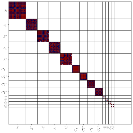
Figure 2: The block diagonal structure of the reduced density matrix with 13 blocks.

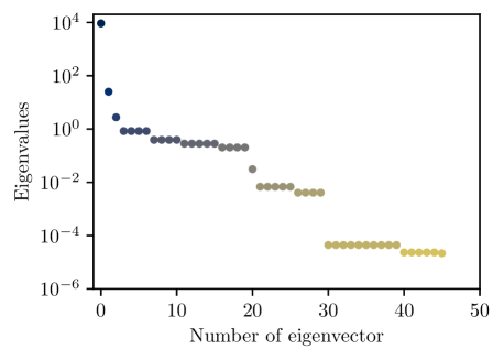
Figure 3: The eigenvalues of the density matrix.

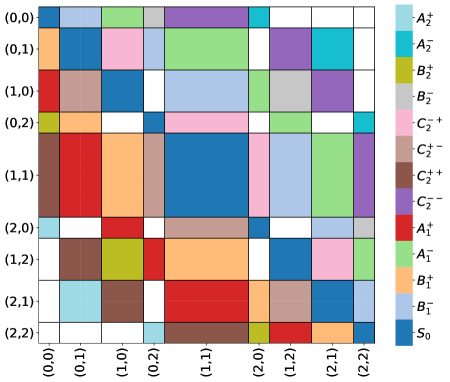
Figure 4: The sparse structure of the SPOs obtained by diagonalizing density matrix. Here, we show the SPOs of an FS-DOF consists of 4 spin (2 alpha and 2 beta) orbitals with 16 configurations. All 13 basic types of SPOs are shown in different colors. The non-zero elements of different SPO matrices are only within the blocks of the corresponding color.

Figure 2 shows, as an example, the block diagonal structure of the reduced density matrix for the FS-DOF consisting of four occupied spin MOs of LiH using the STO-3G basis. The eigenvalues of the density matrix, shown in Fig. 3, provide insight into the significance of the corresponding SPO and offer an estimate of how many should be utilized. In this numerical example, given the rapid decrease in eigenvalues, it is anticipated that numerical convergence can be achieved with fewer (10-15) SPOs.

Due to its block structure, it is not necessary to compute the full density matrix, potentially a very expensive task, and indeed in practice one only needs to evaluate these 13 blocks and diagonalize them separately to obtain the SPOs. Additionally, due to the block structure of the operator density matrix, its eigenvectors are very sparse, and so are the corresponding SPO matrices obtained by folding the latter into 2-index objects. The sparse structure of the SPOs is shown in Fig. 4, where all 13 types of SPO appear in different colors. The corresponding operators have non-zero elements only within the blocks indicated by the corresponding color. Each of the unique 13 types of basis SPO has different physical meaning;
(i) $S_{0}$ SPOs move electrons within different orbitals of the FS-DOF,
(ii) $A_{1}^{+/-}$ SPOs add/remove one alpha electron, respectively,
(iii) $B_{1}^{+/-}$ SPOs add/remove one beta electron, respectively
(iv) $A_{2}^{+/-}$ SPOs add/remove two alpha electrons, respectively
(v) $B_{2}^{+/-}$ SPOs add/remove two beta electrons, respectively
(vi) $C_{2}^{++/--}$ SPOs add/remove one alpha and one beta electron, respectively
(vii) $C_{2}^{+-/-+}$ SPOs add/remove one alpha and remove/add one beta electron.

This structure reveals that many core-tensor elements in a T-SQR operator are zero; only those terms that conserve the particle number are non-zero. For example, in a system with two FS-DOFs, $A_{1}^{+}$ SPOs acting on the first FS-DOF can only be paired with $A_{1}^{-}$ SPOs acting on the second FS-DOF, and the core-tensor element for all 12 other pairs must be zero to conserve the total particle number. Hence, the SPOs obtained from diagonalization of the operator density matrix behave quite similarly to particle creation/annihilation operators (or in general to ladder operators of some kind) acting on the Euclidian space defined by FS-DOF configurations.

II.3.2 Canonical polyadic decomposition (CPD-SQR)

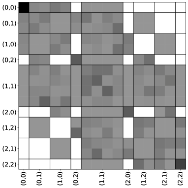
Figure 5: Example of a CPD-SQR single particle operator of an FS-DOF consisting of 4 spin (2 alpha and 2 beta) orbitals with 16 configurations. The single particle operator of a CPD-SQR Hamiltonian does not have any particular sparse structure and can have any form demanded by the minimization algorithm.

The Tucker form grows exponentially with the number of FS-DOFs due to the core-tensor [53]. An alternative is the well-known canonical polyadic decomposition (CPD) also known as CANDECOMP or PARAFAC form in the literature [58, 59, 60, 61, 43]. The CPD form of the SQR (CPD-SQR) electronic Hamiltonian reads

$$H_{z_{1},\ldots,z_{f}}^{\text{CPD}}=\sum_{r=1}^{R}c_{r}\prod_{\kappa=1}^{f}[\mathbf{X}_{r}^{(\kappa)}]_{z_{\kappa}},$$ (26)

where $R$ is the rank of the CPD, $c_{r}$ and $\mathbf{X}_{r}^{(\kappa)}$ are the coefficient and SPO of $\kappa$-th FS-DOF in the $r$-th term of the expansion. The main difference from the Tucker form is that the SPOs acting on the $\kappa$-th degree of freedom are no longer orthogonal to each other (cf. Eq. (14)). This additional freedom makes the CPD form a very compact SOP representation of the tensor. On the other hand, this also makes the CPD much harder to obtain. The numerical challenge is to find both the coefficient and the SPOs, and often the so-called alternating least squares (ALS) method is used. This is our approach as outlined in Section II.4.

When comparing the structure of the SPOs obtained from T-SQR and CPD-SQR it becomes quite clear that CPD-SQR can achieve a more compact form of the sum-of-products operator. As discussed when considering the density matrix in Fig. 2, each of the 13 basic types of SPOs performs a specific task (e.g. annihilating an $\alpha$-electron from the corresponding FS-DOF), which is reflected in the sparse structure of the corresponding matrix representations of the SPOs, Fig. 4. On the other hand, the SPOs in a compactified CPD-SQR are no longer constrained by the orthogonality condition and, in general, can assume any form dictated by the minimization procedures. In particular, they can no longer be ascribed to any of the previously discussed operator categories, as seen by inspecting Fig. 5. This additional freedom of the SPOs, not being members of an orthonormal basis of operators, will prove crucial in achieving a very compact representation of the SQR operator.

II.3.3 Relation to matrix product operators

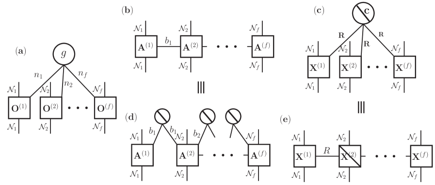
Figure 6: Diagrams for various sum-of-products operators. The square box and circle are single particle operators and core tensors, respectively. The connected lines are contracted indices and disconnected lines are the primitive indices. The diagonal line within a box or circle indicates the contracted indices connecting SPOs or core tensors are diagonal. T-SQR, MPO, and CPD-SQR forms are shown in (a), (b), and (c), respectively. Alternative forms of MPO and CPD-SQR are shown in (d) and (e), respectively.

There is yet another SOP form of the operator, the matrix product operator (MPO) [31, 32, 33, 34, 35, 36]. The MPO form of the electronic Hamiltonian reads

$$H_{z_{1},\ldots,z_{f}}^{\text{MPO}}=\sum_{\alpha}[\mathbf{A}_{\alpha_{1}}^{(1)}]_{z_{1}}\cdots[\mathbf{A}_{\alpha_{\kappa-1},\alpha_{\kappa}}^{(\kappa)}]_{z_{\kappa}}\cdots[\mathbf{A}_{\alpha_{f-1}}^{(f)}]_{z_{f}},$$ (27)

where, $\alpha$ is a combined index of ($\alpha_{1},\ldots,\alpha_{f-1}$) and $\mathbf{A}_{\alpha_{\kappa-1},\alpha_{\kappa}}^{(\kappa)}$ are operators acting on site $\kappa$, henceforth equivalent to the SPO introduced above and referred to as such in the following. The non-terminal SPOs have two indices, one shared with the tensor to its left and the other with the tensor to its right side.

From the point of view of tensor decomposition, the MPO can be viewed as an intermediate between the Tucker decomposition and the CPD. The Tucker, MPO, and CPD diagrammatic forms are shown in Fig. 6 (a), (b), and (c), respectively. The square boxes and circles indicate SPOs and core tensors, respectively. The connecting lines correspond to contracted (summed) indices and disconnected lines indicate primitive indices, i.e., indices of the original tensor. Diagonal lines within the boxes or circles indicate that the corresponding tensor is diagonal in the indices connecting SPOs or core tensors (and not the primitive indices). In Tucker format (Fig. 6(a)), the core tensor coefficients $g$ are contraction coefficients multiplying the SPOs of all FS-DOF, thus the exponential scaling of this form. In an MPO, only neighboring SPOs are connected (Fig. 6(b)). From the perspective of a Tucker form, this can be viewed as if a two-dimensional diagonal core tensor (i.e., a diagonal matrix) connects them, as depicted in Fig. 6(d). Similarly, from the perspective of a Tucker form the CPD form (Fig. 6(c)) can be regarded as possessing a diagonal core tensor, so all connecting lines count with the same index. Alternatively, one can view the CPD as an MPO where the $\mathbf{A}_{\alpha_{\kappa-1},\alpha_{\kappa}}^{(\kappa)}$ tensors are diagonal in the $\alpha$ indices, as indicated by the diagonal line in the non-terminal diagonal boxes in Fig. 6(d).

The MPO form of the Hamiltonian may turn out to be very efficient at capturing couplings between neighboring sites and, as in the matrix product state representation of the wavefunction, it may be advantageous if the physical system has a connectivity that is well-suited to the topology of the MPO tensor representation. On the other hand, a CPD operator is, in principle, free from such restraint. However, the ansatz of the wavefunction determines to a large extent what form of the Hamiltonian constitutes an optimal choice from a numerical perspective, and the MPO form of the Hamiltonian is compatible with the matrix product states (MPS) representation of the wavefunction [31, 32, 33, 34, 35, 36]. Our ML-MCTDH implementation works efficiently with general SOPs and, in principle, it is possible to unfold an MPO and use it with MCTDH. It is yet to be investigated if the (ML-)MCTDH ansatz and algorithm can profit from the MPO structure in some way that does not involve its trivial unfolding into the explicit enumeration of all product terms contained in Eq. (27). This question is beyond the scope of this work.

II.4 Obtaining compact CPD-SQR operators via ALS

II.4.1 General approach to finding an optimal CPD

Before discussing the ALS method in detail, let us introduce a number of quantities. Following the notation written in Eq. (II.3.1), let

$$[\Omega_{r}]_{Z}=\prod_{\kappa}[\mathbf{X}_{r}^{(\kappa)}]_{z_{\kappa}}$$ (28)

be the product of all SPOs for one expansion term r and matrix element $Z=(z_{1},z_{2},\ldots)$, then the CPD form of the Hamiltonian (26) can be rewritten as

$$H_{Z}^{\text{CPD}}=\sum_{r}c_{r}[\Omega_{r}]_{Z}.$$ (29)

Let us also define the single-hole product of all SPOs

$$[\Omega_{r}^{\kappa}]_{Z^{\kappa}}=\prod_{\kappa^{\prime}\neq\kappa}[\mathbf{X}_{r}^{(\kappa^{\prime})}]_{z_{\kappa^{\prime}}}.$$ (30)

Let us further define the positive semidefinite single-hole overlap matrices

$$S_{r,r^{\prime}}^{(\kappa)}=\sum_{Z^{\kappa}}[\Omega_{r}^{\kappa}]_{Z^{\kappa}}[\Omega_{r^{\prime}}^{\kappa}]_{Z^{\kappa}},$$ (31)

which are separable, i.e.,

$$S_{r,r^{\prime}}^{(\kappa)}=\prod_{\kappa^{\prime}\neq\kappa}\zeta_{r,r^{\prime}}^{(\kappa^{\prime})},$$ (32)

where

$$\zeta_{r,r^{\prime}}^{(\kappa^{\prime})}=\sum_{z_{\kappa^{\prime}}}[\mathbf{X}_{r}^{(\kappa^{\prime})}]_{z_{\kappa^{\prime}}}[\mathbf{X}_{r^{\prime}}^{(\kappa^{\prime})}]_{z_{\kappa^{\prime}}},$$ (33)

which can be exploited for numerical calculation. To obtain coefficients and SPOs, one defines a functional $J$ that is to be optimized as

$$\mathcal{J}=\sum_{Z}(H_{Z}-H_{Z}^{\text{CPD}})^{2}+\epsilon\sum_{r}c_{r}^{2}\sum_{Z}[\Omega_{r}]_{Z}^{2}.$$ (34)

Here the first term measures the error of the CPD-SQR expansion, Eq. (26), with respect to the original Hamiltonian, and the second term serves as a regularization term with regularization parameter $\epsilon$. It is introduced to avoid the appearance of linear dependent terms in the CPD expansion during the optimization. The regularization parameter $\epsilon$ is set to a small number, usually the square root of machine precision, i.e. $\epsilon=10^{-8}$. The functional derivative of $\mathcal{J}$ with respect to the SPO of one FS-DOF times the coefficient yields

$$\frac{\delta\mathcal{J}}{\delta c_{r}[\mathbf{X}_{r}^{(\kappa)}]_{z_{\kappa}}}= -2\sum_{Z^{\kappa}}H_{Z}[\Omega_{r}^{\kappa}]_{Z^{\kappa}}+2\sum_{r^{\prime}}c_{r^{\prime}}[\mathbf{X}_{r}^{(\kappa)}]_{z_{\kappa}}S_{r,r^{\prime}}^{(\kappa)}$$

$$+2\epsilon c_{r}[\mathbf{X}_{r}^{(\kappa)}]_{z_{\kappa}}S_{r,r}^{(\kappa)}\longmapsto 0.$$ (35)

Now one can define

$$[x_{r}^{(\kappa)}]_{z_{\kappa}}=c_{r}[\mathbf{X}_{r}^{(\kappa)}]_{z_{\kappa}}$$

$$[b_{r}^{(\kappa)}]_{z_{\kappa}}=\sum_{Z^{\kappa}}H_{Z}\,[\Omega_{r}^{\kappa}]_{Z^{\kappa}}$$ (36)

to arrive at the following working equations for obtaining optimal coefficients and SPOs of the $\kappa$-th FS-DOF

$$[b_{r}^{(\kappa)}]_{z_{\kappa}}=\sum_{r^{\prime}}\left(S_{r,r^{\prime}}^{(\kappa)}+\epsilon\delta_{r,r^{\prime}}\right)[x_{r^{\prime}}^{(\kappa)}]_{z_{\kappa}}.$$ (37)

The above equation is a linear equation with respect to $r$ and can be solved with standard linear algebra tools. Note that in Eq.( 37), the solution for one FS-DOF $\kappa$ depends on the solution of all other FS-DOFs via the single hole overlap matrix $\mathbf{S}^{(\kappa)}$. Therefore, one needs to solve it iteratively from an initial guess tensor, which constitutes the aforementioned ALS method.

In the most general case, a major bottleneck of the above procedure is Eq. (II.4.1), for $b^{(\kappa)}$ contains a multidimensional sum over index $Z^{\kappa}$ (i.e. overall tensor elements except one) which in general cannot be separated into products of the low dimensional sums. If the dimensionality of the system becomes too large, these sums become very expensive and quickly unaffordable, especially since they need to be done multiple times in each ALS iteration. Additionally, one needs to store the full tensor, which grows astronomically with the number of dimensions.

To circumvent this problem one can replace the exact sum (integration) with the Monte Carlo integration scheme. First, a sampling space is prepared by various sampling strategies and then the sum (integration) is done on the sampling space. This is the procedure followed in the Monte Carlo CPD (MCCPD) representation of the potential energy surface [43]. Here, the smoothness of the potential energy surface is exploited in the sense that close grid points have similar energy cuts through the potential.

The generation of a sampling that captures the essence of the SQR electronic Hamiltonian tensor is, however, not practicable, if not impossible. The reason is twofold: (i) The Hamiltonian tensor is very sparse. A sampling must be able to capture both, the zero and non-zero tensor elements in the sampling space and (ii) there is no smoothness relation between neighboring tensor elements such that their values are highly erratic along all dimensions of the tensor. Neighboring rows and columns of the tensor do not, in general, have a similar form. Finding a suitable sampling in this multidimensional space is, hence, a formidable task.

II.4.2 Sum-of-products to sum-of-products for CPD-SQR

For practical purposes, we rely on the fact that the original SQR Hamiltonian is already in a sum-of-products form. This is the Hamiltonian in Eq. (II.1). This Hamiltonian has potentially a very large number of terms as discussed in Section II.1, which makes its direct application very costly. It can, however, be compressed into smaller a CPD-SQR Hamiltonian. Assuming that the original Hamiltonian has already the desired sum-of-products form, the summation over $Z^{\kappa}$, Eq. (II.4.1), factorizes into sums of products of summations over $z_{\kappa}$, which renders the summation not only numerically affordable but also parallelizable. Hence, the purpose of the CPD-SQR procedure outlined below is to find a much more compact sum-of-products form than the original Hamiltonian while maintaining control over the accuracy of the compressed operator.

Therefore, first, we discuss how to generate an exact sum-of-product form of the SQR Hamiltonian that can be used as a starting point for the compactification procedure. In the FS-DOF primitive basis, all terms of Eq. (II.1) that act only within the spin orbitals of one FS-DOF can be summed up to form an uncorrelated operator term. Similarly, one can form correlated operators (products acting on two or more FS-DOF) by summing all terms that act within one FS-DOF for each distinct string operating on the spin orbitals of the other FS-DOF. The compact form of the SQR Hamiltonian for an arbitrary FS-DOF combination is given in Ref. 53 and called the summed SQR (S-SQR) Hamiltonian. The S-SQR form of the Hamiltonian is exact within the space of configurations spanned by the different FS-DOFs. Since the matrix operators acting on each FS-DOF and for different products are not related to each other, this form of the SQR operator is de facto an exact CPD:

$$H_{z_{1},\ldots,z_{f}}=\sum_{s=1}^{R_{e}}\prod_{\kappa=1}^{f}[\mathbf{Y}_{s}^{(\kappa)}]_{z_{\kappa}}.$$ (38)

Once, the SQR Hamiltonian is written as an exact SOP form (Eq. 38), Eq.( II.4.1) can be written by means of separable terms, to be exploited in numerical calculations

$$[b_{r}^{(\kappa)}]_{z_{\kappa}} =\sum_{Z^{\kappa}}H_{Z}[\Omega_{r}^{\kappa}]_{Z^{\kappa}}$$

$$=\sum_{r^{\prime}}^{R_{e}}[\mathbf{Y}_{r^{\prime}}^{(\kappa)}]_{z_{\kappa}}\prod_{\kappa^{\prime}\neq\kappa}\sum_{z_{\kappa^{\prime}}}[\mathbf{Y}_{r^{\prime}}^{(\kappa^{\prime})}]_{z_{\kappa^{\prime}}}[\mathbf{X}_{r}^{(\kappa^{\prime})}]_{z_{\kappa^{\prime}}}.$$ (39)

With Eq. (39) one may now straightforwardly implement the ALS algorithm and obtain a more compact SOP form of the Hamiltonian. At this stage, however, the resulting CPD-SQR Hamiltonian is not guaranteed to be Hermitian. This is even true if all SPO $\mathbf{X}_{r}^{(\kappa)}$ of the initial guess tensor are chosen Hermitian (apart from special cases where all operators $b_{r}^{(\kappa)}$ are Hermitian). A simple workaround is the a posteriory symmetrization of the CPD-SQR Hamiltonian. This, however, doubles the number of terms. Hence, we use a symmetrized ansatz for the CPD-SQR Hamiltonian and adapt the ALS algorithm to preserve Hermiticity during the optimization. We assume

$$H^{\text{CPD}} =\sum_{r}^{R/2}c_{r}\prod_{\kappa}\mathbf{X}_{r}^{(\kappa)}+\sum_{r}^{R/2}c_{r}^{*}\prod_{\kappa}\left(\mathbf{X}_{r}^{(\kappa)}\right)^{\dagger}$$ (40)

$$=\sum_{r}^{R}\tilde{c}_{r}\tilde{\mathbf{X}}_{r}^{(\kappa)},$$ (41)

i.e., we split the total sum into two parts, one part containing operators and coefficients to be found and a second part being the Hermitian conjugate of the first. The sum in the second line, Eq. (41) simply runs over both sums in Eq. (40) where we assume that the Hermitian conjugate terms have indices $r=R/2+1,\cdots,R$.

Note that Hermitian conjugation of the complete $H^{\rm CPD}$, Eq. (41), is equivalent to swapping the positions of the terms $r$ and $r+R/2$, that is, the Hermitian conjugate terms now have indices $r=1,\cdots,R/2$, and the original terms have indices $r>R/2$. The result of the sum is the same, of course.

If the two different orders of the summation (with and without Hermitian conjugation) are inserted into Eq. (35) and following, the single-hole overlaps (assuming all operators and all $\tilde{c}_{r}$ are real) obey the permutation rules

$$S^{(\kappa)}_{r,r^{\prime}} =S^{(\kappa)}_{r+R/2,r^{\prime}+R/2},$$ (42)

$$S^{(\kappa)}_{r,r^{\prime}+R/2} =S^{(\kappa)}_{r+R/2,r^{\prime}}.$$ (43)

If Eq. 40 should hold, one must also obtain

$$b_{r}^{(\kappa)}=\left(b_{r+R/2}^{(\kappa)}\right)^{\dagger}.$$ (44)

The latter permutation rule, Eq. (44), is usually not fulfilled when calculating $b_{r}^{(\kappa)}$ in Eq. (II.4.1), even when starting from a Hermitian initial guess. We hence enforce Eq. (44) by symmetrizing the quantities $S^{(\kappa)}$ and $b^{(\kappa)}$ in Eq. (40) in each iteration step according to Eqs. (42) to (44). Thereafter, solving Eq. (37) with symmetrized $S^{(\kappa)}$ and $b^{(\kappa)}$ leads to a Hermitian CPD-SQR Hamiltonian in the form of Eq. (40). Note that, differently from an a posteriory Hermitization of the optimized Hamiltonian $H^{\rm CPD}$ according to Eq. (40), here both, the original and the Hermitian conjugate SPOs, enter the working equations such that the optimization result is adapted to the ansatz Eq. (40).

We implemented the scheme outlined above, which proved to be working but is numerically expensive as relatively large matrices need to be stored and processed. Especially calculating the single-hole overlap matrices $S^{(\kappa)}$ is expensive, even though many temporary results, for instance, Eq. (33), can be re-used for several modes. Hence, we pick up the idea of finding a minimal but (almost) optimal and orthogonal basis of elementary operators $\mathbf{\Gamma}^{(\kappa)}_{\alpha_{\kappa}}$ such that any single particle operator of the original Hamiltonian can be expressed as a liner combination of elementary operators as

$$[\mathbf{Y}_{r^{\prime}}^{(\kappa)}]_{z_{\kappa}}=\sum_{\alpha_{\kappa}}^{g_{\kappa}}a_{r^{\prime},\alpha_{\kappa}}[\mathbf{\Gamma}^{(\kappa)}_{\alpha_{\kappa}}]_{z_{\kappa}}$$ (45)

with the expansion coefficients

$$a_{r,\alpha_{\kappa}}=\sum_{z_{\kappa}}[\mathbf{\Gamma}^{(\kappa)}_{\alpha_{\kappa}}]_{z_{\kappa}}[\mathbf{Y}_{r}^{(\kappa)}]_{z_{\kappa}}$$ (46)

and expansion order $g_{\kappa}$. Of course, the SPO $\mathbf{X}_{r}^{(\kappa)}$ of $H^{\rm CPD}$ are also linear combinations of the same basis operators

$$[\mathbf{X}_{r}^{(\kappa)}]_{z_{\kappa}}=\sum_{\alpha_{\kappa}}^{g_{\kappa}}c_{r,\alpha_{\kappa}}[\mathbf{\Gamma}^{(\kappa)}_{\alpha_{\kappa}}]_{z_{\kappa}}$$ (47)

as well as the single-hole overlaps of $H^{\rm CPD}$ with the original Hamiltonian

$$[b_{r}^{(\kappa)}]_{z_{\kappa}}=\sum_{\alpha_{\kappa}}^{g_{\kappa}}d_{r,\alpha_{\kappa}}[\mathbf{\Gamma}^{(\kappa)}_{\alpha_{\kappa}}]_{z_{\kappa}}.$$ (48)

Here one hopes that the expansion order is much smaller than the number of matrix elements in the SPOs such that the overlaps in Eq. (33) can be expressed as

$$\zeta_{r,r^{\prime}}^{(\kappa^{\prime})} =\sum_{z_{\kappa}}[\mathbf{X}_{r}^{(\kappa)}]_{z_{\kappa}}[\mathbf{X}_{r^{\prime}}^{(\kappa)}]_{z_{\kappa}}$$ (49)

$$=\sum_{\alpha_{\kappa}}^{g_{\kappa}}c_{r,\alpha_{\kappa}}c_{r^{\prime},\alpha_{\kappa}}$$ (50)

which are dot-products of small vectors as opposed to large matrices. Similarly, Eq. (39) becomes after multiplication with $\mathbf{\Gamma}^{(\kappa)}_{\alpha_{\kappa}}$ from the left and subsequent summation over $z_{\kappa}$

$$d_{r,\alpha_{\kappa}} =\sum_{r^{\prime}}^{R_{e}}a_{r^{\prime},\alpha_{\kappa}}\prod_{\kappa^{\prime}\neq\kappa}\sum_{\alpha_{\kappa}}^{g_{\kappa}}a_{r^{\prime},\alpha_{\kappa^{\prime}}}c_{r,\alpha_{\kappa^{\prime}}},$$ (51)

again only involving small dot-products.

In practice, the basis operators $\Gamma^{(\kappa)}_{\alpha_{\kappa}}$ are not obtained via diagonalization of the density matrix, Eq. (18), as done for the Tucker decomposition, because calculating the density matrix is numerically expensive, but by re-shaping all $\mathbf{Y}_{r^{\prime}}^{(\kappa)}$ into vectors and arranging them into columns of a possibly large matrix $U^{(\kappa)}$ of size $\mathcal{N}^{2}_{\kappa}\times R_{e}$. Subsequently the $g_{\kappa}$ most important left singular vectors and values $\sigma_{\alpha_{\kappa}}$ are computed, where $g_{\kappa}$ is determined by a pre-set cut-off $\epsilon_{\rm SVD}$ (typically set to $10^{-9}$) such that

$$\frac{\sum\limits_{\alpha_{\kappa}=g_{\kappa}+1}^{\mathcal{N}_{\kappa}^{2}}\sigma_{\alpha_{\kappa}}^{2}}{\sum\limits_{\alpha_{\kappa}=1}^{\mathcal{N}_{\kappa}^{2}}\sigma_{\alpha_{\kappa}}^{2}}<\epsilon_{\rm SVD}.$$ (52)

The respective left singular vectors are reshaped into the matrices $\mathbf{\Gamma}^{(\kappa)}_{\alpha_{\kappa}}$ and serve as basis operators. This has to be done only once at the beginning of the calculation. The ALS optimization is hence performed in a much smaller vector space than the original SPOs are defined in, which saves net computational effort. Only at the very end of the calculation, the operators $\mathbf{X}_{r}^{(\kappa)}$ are reconstructed using Eq. (47).

A major drawback of this procedure is, however, that Hermiticity cannot be restored with the recipe outlined above. Here we resort to a different strategy. As in all of the formulas above, we assume that the matrix elements $[\mathbf{Y}_{r^{\prime}}^{(\kappa)}]_{z_{\kappa}}$ of the original SPOs are real. We can then decompose all SPOs into a symmetric (Hermitian) part ${}^{\rm S}\mathbf{Y}_{r^{\prime}}^{(\kappa)}$ and an anti-symmetric (anti-Hermitian) part ${}^{\rm A}\mathbf{Y}_{r^{\prime}}^{(\kappa)}$

$$\mathbf{Y}_{r^{\prime}}^{(\kappa)}={}^{\rm S}\mathbf{Y}_{r^{\prime}}^{(\kappa)}+{}^{\rm A}\mathbf{Y}_{r^{\prime}}^{(\kappa)}$$ (53)

Furthermore, one may realize that

$$\sum_{z_{\kappa}}\left[{}^{\rm S}\mathbf{Y}_{r^{\prime}}^{(\kappa)}\right]_{z_{\kappa}}\cdot\left[{}^{\rm A}\mathbf{Y}_{r^{\prime}}^{(\kappa)}\right]_{z_{\kappa}}=0$$ (54)

for any symmetric and anti-symmetric matrices. We can then repeat the procedure to obtain elementary operators as outlined above, but separately for the symmetric and the anti-symmetric operators, i.e, all symmetric matrices ${}^{\rm S}\mathbf{Y}_{r^{\prime}}^{(\kappa)}$ are reshaped into vectors and arranged into columns of a matrix ${}^{\rm S}\mathbf{U}_{r^{\prime}}^{(\kappa)}$ and all anti-symmetric matrices ${}^{\rm A}\mathbf{Y}_{r^{\prime}}^{(\kappa)}$ are reshaped into vectors and arranged into columns of a matrix ${}^{\rm A}\mathbf{U}_{r^{\prime}}^{(\kappa)}$ from which ${}^{\rm S}g_{\kappa}$ symmetric and ${}^{\rm A}g_{\kappa}$ anti-symmetric left singular vectors (elementary operators) ${}^{\rm S}\mathbf{\Gamma}^{(\kappa)}_{\alpha_{\kappa}}$ and ${}^{\rm A}\mathbf{\Gamma}^{(\kappa)}_{\beta_{\kappa}}$ are computed, respectively. The combined set, $\left\{{}^{\rm S}\mathbf{\Gamma}a^{(\kappa)}_{\alpha_{\kappa}},{}^{\rm A}\mathbf{\Gamma}^{(\kappa)}_{\beta_{\kappa}}\right\}$ hence forms an orthonormal basis and such that

$$[\mathbf{Y}_{r^{\prime}}^{(\kappa)}]_{z_{\kappa}} =\sum_{\alpha_{\kappa}=1}^{{}^{\rm S}g_{\kappa}}{}^{\rm S}a_{r^{\prime},\alpha_{\kappa}}[^{\rm S}\mathbf{\Gamma}^{(\kappa)}_{\alpha_{\kappa}}]_{z_{\kappa}}+\sum_{\beta_{\kappa}=1}^{{}^{\rm A}g_{\kappa}}{}^{\rm A}a_{r^{\prime},\beta_{\kappa}}[^{\rm A}\mathbf{\Gamma}^{(\kappa)}_{\beta_{\kappa}}]_{z_{\kappa}}$$ (55)

$$=\sum_{\gamma_{\kappa}=1}^{\bar{g}_{\kappa}={}^{\rm S}g_{\kappa}+{}^{\rm A}g_{\kappa}}\bar{a}_{r^{\prime},\gamma_{\kappa}}[\mathbf{\bar{\Gamma}}^{(\kappa)}_{\gamma_{\kappa}}]_{z_{\kappa}}$$ (56)

with expansion coefficients ${}^{\rm S}a_{r^{\prime},\alpha_{\kappa}}$ and ${}^{\rm A}a_{r^{\prime},\beta_{\kappa}}$ for the symmetric and anti-symmetric elementary operators respectively (or combined expansion coefficients $\bar{a}_{r^{\prime},\gamma_{\kappa}}$ for the combined set of basis operators). Similar formulas hold for $\mathbf{X}_{r}^{(\kappa)}$ and $b_{r}^{(\kappa)}$. The Hermitian conjugate of the expansion, Eq. (56) is obtained by simply swapping the sign of the coefficients ${}^{\rm A}a_{r^{\prime},\beta_{\kappa}}$ of the anti-symmetric basis operators.

We are now in a position to return to the ansatz Eq. (40) and repeat the derivations, Eqs. (44) to (51). One realizes that the optimization procedure can again be performed entirely in the vector space of the expansion coefficients and the symmetrization of Eq. (44) is simply performed by swapping the sign of the coefficients of the anti-symmetric basis operators.

Note furthermore, that only non-zero vectors ${}^{\rm S}\mathbf{Y}_{r^{\prime}}^{(\kappa)}$ and ${}^{\rm A}\mathbf{Y}_{r^{\prime}}^{(\kappa)}$ need to be stored in the matrices ${}^{\rm S}\mathbf{U}_{r^{\prime}}^{(\kappa)}$ and ${}^{\rm A}\mathbf{U}_{r^{\prime}}^{(\kappa)}$, respectively. If all ${}^{\rm A}\mathbf{Y}_{r^{\prime}}^{(\kappa)}=0$ (i.e., all SPO of the original Hamiltonian are Hermitian) the fit $H^{\rm CPD}$ is obtained Hermitian automatically without Ansatz Eq. (40) irrespective of whether the reduction, Eq. (45) is used.

We have implemented the SOP-to-SOP algorithms outlined above in a new program compactoper as part of the Heidelberg MCTDH package [62]. An important comment related to its general application to nuclear dynamics problems should be added here: While the procedure outlined above works in general for any operators in sum-of-products form in the sense that it leads to (much) fewer terms in the sum, the resulting operator may turn out not to be the optimal form to perform dynamics calculations. For instance, kinetic energy operators in polyspherical coordinates[63, 64] may, depending on the molecule under consideration, contain thousands of product terms.[65] Many of the single particle operators are, however, unit operators or diagonal operators that depend on a single coordinate and require none or little numerical effort to operate on the wave function. The procedure above, however, will return all single particle operators in matrix form, which are expensive to operate. Operating the kinetic energy in its original form would usually by far outperform operating its compacted form obtained with the schemes outlined above. One should, hence, use this method only if the vast majority of SPOs of the original Hamiltonian are matrices in the first place, as is the case for the SQR calculations shown below, or if all SPOs are diagonal in the first place, i.e., if the Hamiltonian is a potential (in this case, our implementation uses vectors of single-particle potentials instead of matrices of single-particle operators).

III Numerical examples

The ab initio MCTDH-SQR approach can be directly applied to the calculation of electronic excitation or ionization spectra of molecular systems through time propagation instead of matrix diagonalization. For this, one needs to prepare an appropriate initial state (ionized and excited in cases of ionization and excitation spectrum, respectively) that overlaps with the desired state for time-propagation. Then, the power spectrum can be obtained as usual from the Fourier transform of the autocorrelation function

$$\sigma(E)=\frac{1}{\pi}Re\int_{0}^{\infty}e^{iEt}\langle\Psi|\Psi(t)\rangle dt.$$ (57)

Here we benchmark the method on water, trans-polyene, and glycine.

III.1 H₂O

III.1.1 Ionization

We compare the compactness of the T-SQR and CPD-SQR Hamiltonian first by considering the ionization spectrum of the H₂O molecule as a benchmark. The molecular orbitals (MO) are generated using the 6-31G atomic basis for both O and H, and the lowest energy MO (1s of O) is frozen. The remaining 12 spatial orbitals are considered for the calculation. The scheme of FS-DOFs and the corresponding active spaces are given in Table 1.

Table 1: FS-DOFs and active spaces for the ionization spectrum calculation of H₂O.

FS-DOF	No. spat. orb.	Occupations			No. conf.
		alpha	beta	Total
I	4	2-4	2-4	6-8	37
II	4	0-2	0-2	0-2	37
III	4	0-2	0-2	0-2	37

The atomic basis and FS-DOFs are the same as in Ref. 53, where we compiled the S-SQR and T-SQR results. The total number of terms in the original SQR Hamiltonian is 40618, which goes down to 6890 when summed up without approximations, namely the S-SQR (exact CPD).

The initial wavefunction for the propagation is generated by applying the ionization operator

$$\hat{A}=\sum_{i=1}^{4}\sum_{\sigma=\uparrow,\downarrow}\hat{a}_{i,\sigma}$$ (58)

to the ground electronic state of neutral H₂O. This initial wavefunction is a spin doublet and a linear combination of singly-ionized configurations.

Table 2: Number of Hamiltonian terms and wall-clock time for the different sum-of-product form of the Hamiltonian. The wall-clock time is given for 20 fs time propagation. The calculations have been performed with 16 CPUs using shared-memory parallelization on the same machine and CPU type, namely, Dual-Core Intel Xeon, processor type E5-2650 v2 running at 2.6 GHz and the wall-clock times are intended for their relative comparison only. The SQR, S-SQR, and T-SQR results are reproduced from J. Chem. Phys. 157, 134102 (2022) [Ref. 53].

Method	Hamil. terms	Time (h:m)
SQR	40618	243:08
S-SQR	6890	58:21
T-SQR	45000	404:29
CPD-SQR	200	2.08
	400	3.33
	500	4.08
	600	4.48

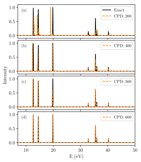
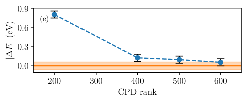
Figure 7: Convergence of electronic ionization spectra of H₂O with different CPD rank. The spectrum in black is calculated with the exact Hamiltonian. The spectra in red are calculated with CPD-SQR Hamiltonian with 200, 400, 500, and 600 CPD ranks and shown in (a), (b), (c), and (d), respectively. The convergence of the 3rd peak (centered around 20 eV) with respect to the CPD rank is shown in (e). The error bar represents the spectral resolution, full width at half maximum (FWHM), stemming from the propagation time. The autocorrelation function was propagated for 20 fs, resulting in a FWHM of about 0.1 eV.

Fig. 7 compares the electronic ionization spectrum of H₂O using the exact Hamiltonian with CPD-SQR Hamiltonians of different CPD ranks. As expected, the numerical accuracy of the spectrum increases with increasing CPD terms and the convergence is achieved with only $\sim$ 600 Hamiltonian terms. Table 2 compares the number of Hamiltonian terms and CPU time for different SOP representations of the electronic Hamiltonian. As seen by inspecting Table 2, the CPD-SQR form significantly outperforms T-SQR in achieving a more compact SOP form of the electronic Hamiltonian. In this example, the CPD-SQR compression factors are $\mathcal{R}=68$ and $\mathcal{R}=12$ with respect to the original SQR and S-SQR Hamiltonian, respectively, where $\mathcal{R}$ is defined as the number of terms of the exact Hamiltonian divided by the number of terms of the corresponding compressed Hamiltonian.

III.1.2 Excitation

Table 3: FS-DOFs and active spaces for the excitation spectrum calculation of H₂O.

FS-DOF	No. spat. orb.	Occupations			No. conf.
		alpha	beta	Total
I	4	1-4	1-4	5-8	93
II	4	0-3	0-3	0-3	93
III	5	0-2	0-2	0-2	56
IV	5	0-2	0-2	0-2	56
V	5	0-2	0-2	0-2	56

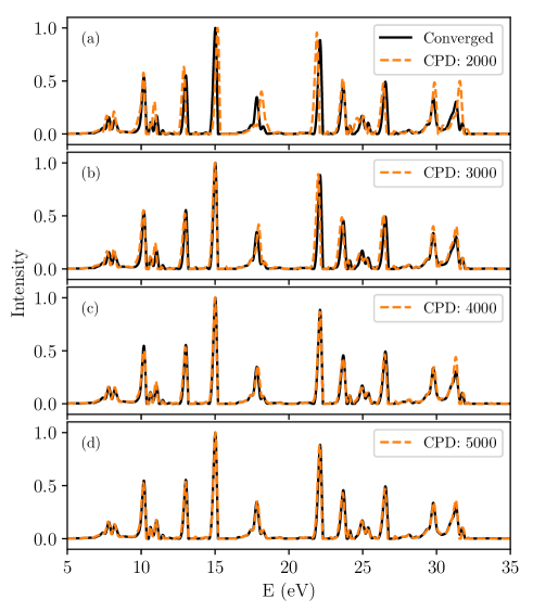
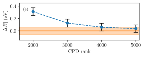
Figure 8: Convergence of electronic excitation spectra of H₂O with different CPD ranks. The spectra in red are calculated with CPD-SQR Hamiltonian with 2000, 3000, 4000, and 5000 CPD rank and shown in (a), (b), (c), and (d), respectively. The numerically converged (regarding Hamiltonian terms) spectra are shown in black and calculated with 10000 CPD rank. Further increases in the CPD rank do not change the spectrum. (e) Convergence of the peak centered around 18 eV with respect to the CPD rank. For details see the caption of Fig 7.

Similarly to ionization, the positions of the low-lying excited states of H₂O can be calculated by time-propagation. In this example, we generate MOs using the cc-pVDZ basis for H and O. The lowest energy MO (1s of O) is frozen and the remaining 46 spin orbitals are considered for the calculation. The scheme of FS-DOFs and the corresponding active spaces are given in Table 3. The initial wavefunction for the propagation is generated by applying the excitation operator

$$\hat{E}=\sum_{i=2}^{4}\sum_{a=5}^{8}\sum_{\sigma=\uparrow,\downarrow}\hat{a}_{a,\sigma}^{\dagger}\hat{a}_{i,\sigma}.$$ (59)

on the ground electronic state of H₂O. The initial wavefunction is a spin-singlet superposition of singly excited configurations and overlaps with many of the low-lying excited singlet states of H₂O. Note that $\hat{E}$ is not the dipole operator and therefore the corresponding excitation spectrum does not correspond to an absorption spectrum, which would contain much fewer peaks. The total number of terms in the original SQR Hamiltonian is 544364 and in the S-SQR Hamiltonian before compression already goes down to 63119 terms. Fig. 8 compares the electronic excitation spectrum of H₂O using CPD-SQR Hamiltonians with increasing rank. The spectrum in black is by far numerically converged with CPD rank 10000. From the figure, it is clear that the convergence is achieved already with about 4000 CPD-SQR Hamiltonian terms. The CPD-SQR compression factor is $\mathcal{R}=136$ and $\mathcal{R}=16$ with respect to the original SQR and S-SQR Hamiltonian, respectively.

Considering now the ML-MCTDH-SQR representation of the electronic wavefunction, the primitive space corresponds to $1.5\cdot 10^{9}$ configurations (product of the rightmost column in Table 3). These can be compared to the $1.6\cdot 10^{5}$ configurations in the Hilbert space of 8 electrons in the restricted Fock space generated by the FS-DOF formation in Table 3. Of course, the ML-MCTDH-SQR ansatz spans a primitive Fock space much larger than the Hilbert space of the relevant electronic number. However, the number of propagated wavefunction coefficients is $\sim 2\cdot 10^{4}$ which is significantly smaller than the number of CI coefficients.

III.2 Trans-C₈H₁₀

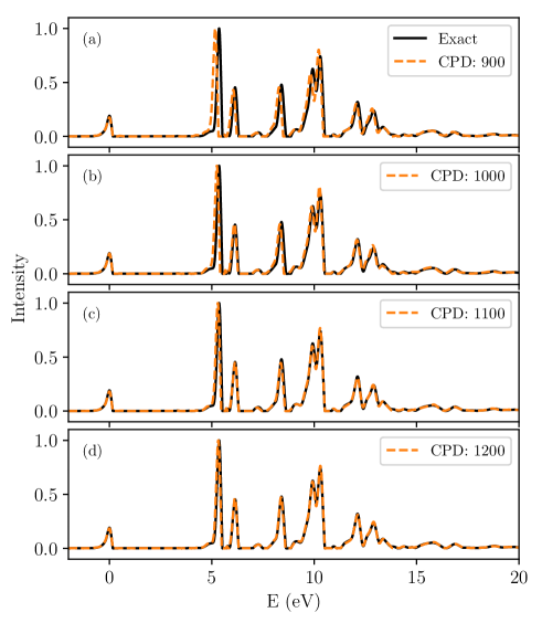
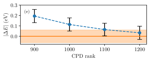
Figure 9: Convergence of excitation spectra of trans-C₈H₁₀ with different CPD rank. The spectrum in black is calculated with the exact Hamiltonian. The spectra in red are calculated with CPD-SQR Hamiltonian with 900, 1000, 1100, and 1200 CPD ranks and shown in (a), (b), (c), and (d), respectively. (e) Convergence of the peak centered around 5 eV (1st excited state) with respect to the CPD rank. For details see the caption of Fig 7.

In the following, we obtain the low-lying $\pi$-excited states of trans-C₈H₁₀. The geometry of C₈H₁₀ is taken to be all trans and is optimized at the B3LYP/cc-pVDZ label of theory and the MOs are calculated using the cc-pVDZ basis for C and H. The orbital space is chosen to be $\pi$-doublet valence, i.e., 8 $\pi$ electrons in 16 $\pi$ spatial (32 spin) orbitals, and the details of the FS-DOF partitioning and active spaces are given in Table 4.

Table 4: FS-DOFs and active spaces for the excitation spectrum calculation of trans-C₈H₁₀.

FS-DOF	No. spat. orb.	Occupations			No. conf.
		alpha	beta	Total
I	4	1-4	1-4	5-8	93
II	4	0-3	0-3	0-3	93
III	4	0-2	0-2	0-2	37
IV	4	0-2	0-2	0-2	37

The initially excited wavefunction is generated as a superposition of singly-excited configurations covering all combinations of the orbitals HOMO-2 to HOMO and LUMO to LUMO+3. From a total of 123648 terms in the original SQR Hamiltonian, we arrive at an S-SQR (exact CPD) with 14212 terms. The excitation spectrum obtained with different CPD ranks is compared with the spectrum calculated with exact Hamiltonian and shown in Fig 9. The CPD-SQR reaches convergences with about 1100 Hamiltonian terms, whereby calculations with only about 900 terms show a good qualitative agreement with the converged excitation energies.

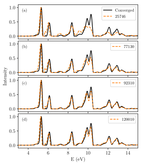
Figure 10: Convergence of excitation spectra of trans-C₈H₁₀ with MCTDH coefficients. The spectrum in black is calculated with the converged MCTDH wavefunction where the lowest natural population of each node of the MCTDH wavefunction is less than $10^{-3}$. The spectra in red are calculated with 25746, 77130, 92130, and 120010 MCTDH coefficients and shown in (a), (b), (c), and (d), respectively.

In this numerical example, the ML-MCTDH-SQR wavefunction consists of $1.2\cdot 10^{7}$ primitive configurations, of which only $4\cdot 10^{4}$ configurations correspond to a Hilbert space of $4$ alpha and $4$ beta electrons. Although the ML-MCTDH wavefunction spans a significantly larger primitive space than the pertinent Hilbert space, the number of propagated MCTDH coefficients can be of the same order or less to get a qualitative agreement with the converged spectrum. Fig. 10 compares the converged spectrum with varying numbers of propagated MCTDH coefficients. The converged calculation is done with MCTDH wavefunction where the lowest natural population of each node is less than $10^{-3}$. It’s clear that even with the MCTDH coefficients (25746) less than the Hilbert space configuration ($4\cdot 10^{4}$), one obtains a qualitatively good agreement.

III.3 Glycine

Table 5: Constructed FS-DOFs for the ionization calculation of glycine molecule

FS-DOF	Spatial orb.	Electron			Conf. No.
		alpha	beta	Total
I	3	1-3	1-3	4-6	22
II	3	1-3	1-3	4-6	22
III	4	1-4	1-4	5-8	93
IV	4	0-3	0-3	0-3	93
V	4	0-2	0-2	0-2	37
VI	5	0-2	0-2	0-2	56

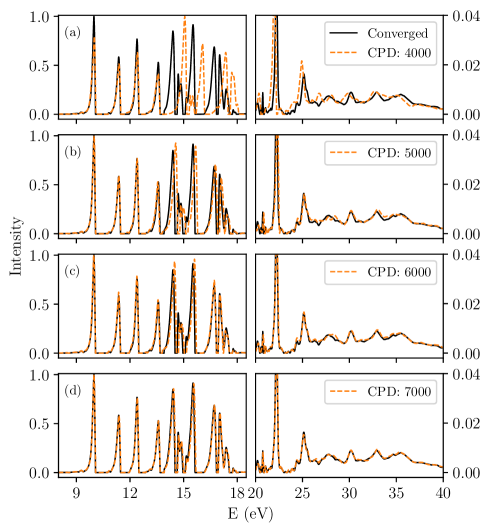
Figure 11: Convergence of electronic ionization spectra of glycine with different CPD rank. The spectra in red are calculated with CPD-SQR Hamiltonian with 4000, 5000, 6000, and 7000 CPD ranks and shown in (a), (b), (c), and (d), respectively. Each plot’s left and right panels show the main peaks (8-18 eV region) and satellite peaks (20-40 eV regions), respectively. The numerically converged (regarding Hamiltonian terms) spectra are shown in black and calculated with 10000 CPD rank. Further increases in the CPD rank do not change the spectrum.

Glycine is one of the smallest amino acids and it has been considered as an example to study charge migration in biological systems using attosecond laser systems. Its ionization spectrum has been studied in the past with the ADC(3) method. Therefore, we consider it and calculate its ionization spectrum and real-time charge migration dynamics using the MCTDH-SQR approach. The cc-pVDZ basis is used for H, C, O, and N to generate the MOs, and we consider 20 electrons in 46 (20 highest occupied and 26 lowest unoccupied) spin orbitals in our calculations. The scheme of FS-DOFs and active spaces is shown in Table 5. The initial wavefunction for the propagation is generated by applying an ionization operator that covers all occupied orbitals to the ground electronic state of neutral glycine. The total number of terms in the original SQR Hamiltonian is now $1.072\cdot 10^{6}$, which can be summed down to $1.11\cdot 10^{5}$ terms. Fig. 11 compares the electronic ionization spectrum of glycine using the CPD-SQR Hamiltonian with increasing ranks. The spectrum in black corresponds to rank $10^{4}$ and is numerically converged. Increasing the rank does not change the spectrum. About 5000 to 6000 terms already provide a very accurate description and 4000 terms is quite accurate in the challenging inner-valence region above 20 eV.

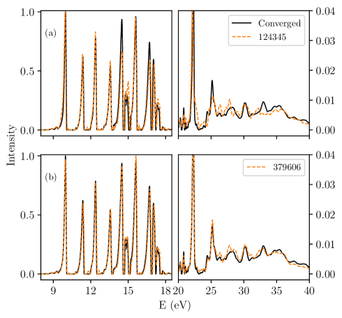
Figure 12: Convergence of electronic ionization spectra of glycine with different propagated ML-MCTDH coefficients. The spectrum in black is calculated with the converged MCTDH wavefunction where the lowest natural population of each node of the MCTDH wavefunction is less than $5\cdot 10^{-4}$. The spectra in red are calculated with 124345 and 379606 propagated ML-MCTDH coefficients and shown in (a) and (b), respectively.

In this example, the adopted FS-DOF scheme, as detailed in Table 5 generates $\sim 8.7\cdot 10^{9}$ primitive configurations. In comparison, the Hilbert space of $10$ alpha and $10$ beta electrons within this Fock space comprises of $\sim 6.2\cdot 10^{8}$ configurations. Furthermore, the numerically converged spectrum of ML-MCTDH is obtained by approximately $5\times 10^{5}$ propagated coefficients, highlighted in black in Fig. 12. Notably, the figure demonstrates that despite a substantial reduction (by more than three orders of magnitude) in the number of ML-MCTDH coefficients (approximately $1.2\times 10^{5}$) compared to the number of CI coefficients ($\sim 6.2\times 10^{8}$), a qualitatively accurate depiction of the ionization spectrum is achieved.

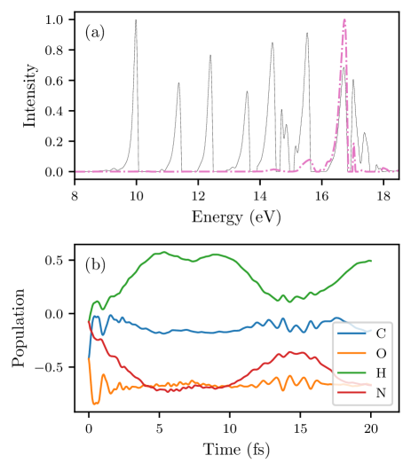
Figure 13: Charge migration dynamics after removal of an electron from HOMO-8 molecular orbital. (a) shows the corresponding signature in the ionization spectra. (b) shows the atomic population dynamics with respect to the initial population of the constituting atoms of glycine.

In the MCTDH-SQR approach, one can naturally extract various time-dependent properties of the system. For example, the ultrafast hole dynamics after the removal of electrons from the HOMO-8 spatial orbitals is shown in Fig. 13. The signature spectrum of the removal of an electron from the HOMO-8 spatial orbital is shown in Fig. 13(a). Fig. 13(b) shows the time-dependent electronic populations of C, O, H, and N atom where the corresponding electronic population of the neutral ground state is subtracted. Therefore, the positive and negative values indicate the presence of extra electrons and holes with respect to the neutral ground state, respectively. These atomic populations are obtained from the MO populations directly available from the propagated ML-MCTDH wavefunctions and their corresponding atomic orbital coefficients. The total electronic population at each point in time is -1, which indicates the presence of one hole in the system. The population at $t=0$ reveals the atomic character of the MO from which the electron is removed. In this case, the HOMO-8 molecular orbital corresponds roughly to 42%, 42%, 8%, and 8% of C, O, H, and N characters, respectively. The initial rapid jump in population in a subfemtosecond time-scale is due to the redistribution of the hole in the presence of an instantaneous electron-electron repulsion [66, 67]. Further, the removal of an electron from the HOMO-8 th orbital breaks down the orbital picture of ionization, which is clear from the multiple peaks in the ionization spectrum  [68]. After the rapid initial rearrangement, the atomic population of carbon and oxygen remain more or less constant, and the hole density hops between nitrogen and hydrogen with a charge migration period of $\sim$ 15 fs. After the first cycle, the H atoms have gained some net electron density whereas the N atom has slightly increased its net hole density.

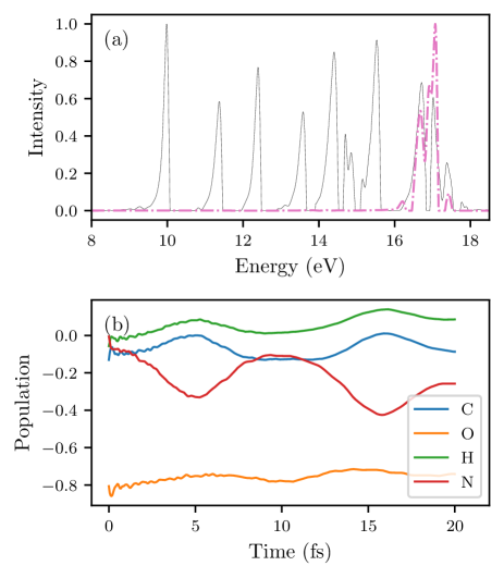
Figure 14: Charge migration dynamics after removal of an electron from HOMO-9 molecular orbital. (a) shows the corresponding signature in the ionization spectra. (b) shows the atomic population dynamics with respect to the initial population of the constituting atoms of glycine.

On the other hand, a different hole dynamics is observed if one removes an electron from HOMO-9 molecular orbital (shown in Fig. 14) and corresponding to an ionization potential of about 17 eV. The HOMO-9 MO is spread to about 13%, 80%, 6%, and 1% onto the C, O, H, and N atoms, respectively. The electronic population at the oxygen atom (where most of the hole lies) remains more or less constant. The rest of the hole density hops between the N atom and its adjacent C and H atoms with a period of about 10 fs. After each cycle, the N atom loses some electronic population and C and H atoms slowly gain electronic population.

These dynamics are susceptible to being probed by ultrafast pump-probe schemes in the attosecond regime. Other approaches such as the ADC(3) method for ionization can provide equivalent information in the frequency domain [69, 70]. An interesting breakthrough for ab initio MCTDH-SQR could be achieved by devising a scheme to consider nuclear displacements at early-times after ionization. This has been demonstrated for one single nuclear coordinate and a simpler SQR Hamiltonian in Ref. 27, and its multidimensional extension shall be the subject of future investigations.

IV Scaling of the ML-MCTDH-SQR method

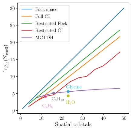
Figure 15: Scaling of various coefficients related to the ML-MCTDH-SQR method with the number of spatial orbitals. The solid lines represent the projected number of coefficients taking into account the underlying assumptions on the wavefunction (see text). The circles represent the total number of propagated ML-MCTDH coefficients, color-coded to denote different numerical examples presented in the text. See supplementary material for the calculation of C₄H₆ system.

Up to now, we focused on the compactification of the CPD-SQR operator. Equally important is the question of how much compactification is achieved for the wavefunction with respect to the primitive configurational space. The MCTDH-SQR primitive space is spanned, in principle, by the $2^{2N}$ configurations in the total Fock space, where N is the number of spatial orbitals (blue line in Fig. 15). However, as previously discussed, practical implementation involves defining an active space within each Fock sub-space based on its maximum and minimum occupation. This effectively constitutes a static pruning of the primitive degrees of freedom. The number of configurations in the selected Fock space is shown in green in Fig. 15. In practice, we often consider sub-Fock spaces formed by four spatial (eight spin) orbitals with an occupation that varies by $\pm 3$ electrons with respect to their reference occupation. The so-selected Fock space corresponds to the actual primitive space (or primitive grid) of the MCTDH calculation. If we consider now that the total occupation of the molecular orbital space is equal to $N/4$, i.e., 75% of the orbitals are virtual in the reference, we can determine the number of configuration interaction (CI) basis states within the corresponding number of electrons. The CI states arising from the full Fock space make up the full CI space shown in orange. The CI states arising from the selected Fock space build up the selected CI space, shown in red. The latter is the important number to be compared with the total number of propagated MCTDH-SQR coefficients. In other words, the primitive space that the MCTDH-SQR tensor-tree spans corresponds to the green trace, but the physical CI space corresponding to a specific number of electrons corresponds to the red trace. Only if the total number of propagated MCTDH-SQR coefficients is substantially lower than the number of selected CI states it is meaningful to undertake an MCTDH-SQR calculation. If they are similar, and it is affordable, it is certainly more efficient to construct the selected CI Hamiltonian and work with it directly.

We have to assume finally how to structure the layering of the ML-MCTDH-SQR wavefunction and the number of SPFs in each layer: we consider balanced trees (as symmetric as possible), where each parent node connects to a maximum of two child nodes (three for the top layer). The number of SPFs in the bottom-layer nodes is set as $1/3$ of the primitive basis size, and the SPF count in a parent node is the sum of the SPFs in its child nodes. Consequently, the number of SPFs increases linearly with the layer of the MCTDH tree. This number as a function of $N$ is shown in purple in Fig. 15. This estimate indicates that for about 20 spatial orbitals and above, the number of ML-MCTDH-SQR coefficients is several orders of magnitude smaller than the number of Hilbert space configurations in the selected CI space of the corresponding number of electrons. This gain increases quickly with the number of spatial orbitals. Crucially, this estimate suggests that an ab initio ML-MCTDH-SQR approach succeeds at compactifying the full-CI state of the system while starting from a much larger Fock space. We note here that, in the ML-MCTDH-SQR approach, no effort whatsoever is made to enforce the wavefunction to the Hilbert space of the problem. Instead, the equations of motion conserve the total number of particles automatically, and this observable becomes de facto a convergence parameter.

V Summary and Conclusion

In this work, we introduce a sum-of-products (SOP) representation for the electronic Hamiltonian within the framework of second quantization (SQR). The quartic scaling of the electronic SQR Hamiltonian with respect to the number of spin orbitals presents a significant challenge when addressing the time-dependent phenomena in large molecular systems. To tackle this issue, we propose a method based on the canonical polyadic decomposition (CPD) to obtain a compact sum-of-product form of the electronic Hamiltonian. In contrast to the Tucker decomposition, the basis functions of a CPD need not be orthogonal to each other, which allows it to create a more compact representation. However, unlike multidimensional potential energy surfaces, the Hamiltonian tensor is highly discontinuous along its dimensions, making it unsuitable for employing a Monte Carlo integration scheme to obtain the CPD form of the Hamiltonian. Here we introduce a practical scheme (SOP to SOP) to obtain the CPD representation of the Hamiltonian. We benchmark our method on H₂O, a trans-polyene, and the ultrafast inner-valence dynamics of ionized glycine, where we demonstrate the compactness of the CPD-SQR Hamiltonian in comparison to the exact Hamiltonian. In particular, CPD-SQR achieves numerical convergence within the spectral resolution of the calculated spectra with a CPD rank of more than two orders of magnitude smaller than the original SQR Hamiltonian. Although the various examples indicate that the accuracy of the state energies improves systematically with the CPD rank, the total accuracy remains limited by the wavefunction propagation time and the corresponding duration of the autocorrelation function. The spectral width in the chosen examples is about 0.1 eV FWHM. We emphasize that our aim with the ML-MCTDH-SQR method and the CPD representation of the operator is to have a variational approach that combines efficiency and robustness to simulate broad spectral ranges for short times, potentially covering regions with very high densities of electronic states (cf. glycine example), whereas high precision and accuracy of single states are of less importance.

A program (named compactoper) implementing the algorithm discussed in this work has been made available in the Heidelberg MCTDH package [62].

VI Supplementary Material

See the supplementary material for the excitation spectrum calculation of trans-C₄H₆ system.

VII Data Availability

The data that support the findings of this study are available within the article and its supplementary material. A program (named compactoper) implementing the algorithm discussed in this work has been made available in the Heidelberg MCTDH package [62].

VIII Acknowledgments

We thank Prof. H.-D. Meyer for the insightful discussions and advice with the MCTDH calculations. We thank Prof. Henrik R. Larsson for discussions on the diagrammatic description of operators. The authors thank JUSTUS 2 in Ulm under grant number bw18K011 for computing time. The authors declare no conflicts of interest.

References

- Meyer, Manthe, and Cederbaum [1990] H. D. Meyer, U. Manthe, and L. S. Cederbaum, “The multi-configurational time-dependent Hartree-approach,” Chem. Phys. Lett. 165, 73 (1990).
- Manthe, Meyer, and Cederbaum [1992] U. Manthe, H.-D. Meyer, and L. S. Cederbaum, “Wave-packet dynamics within the multiconfiguration Hartree framework: General aspects and application to NOCl,” J. Chem. Phys. 97, 3199–3213 (1992).
- Beck et al. [2000] M. H. Beck, A. Jäckle, G. A. Worth, and H.-D. Meyer, “The multiconfiguration time-dependent Hartree method: A highly efficient algorithm for propagating wavepackets.” Phys. Rep. 324, 1–105 (2000).
- Meyer and Worth [2003] H.-D. Meyer and G. A. Worth, “Quantum molecular dynamics: Propagating wavepackets and density operators using the multiconfiguration time-dependent Hartree (MCTDH) method,” Theor. Chem. Acc. 109, 251–267 (2003).
- Meyer, Gatti, and Worth [2009] H.-D. Meyer, F. Gatti, and G. A. Worth, eds., Multidimensional Quantum Dynamics (Wiley, 2009).
- Wang and Thoss [2003] H. Wang and M. Thoss, “Multilayer formulation of the multiconfiguration time-dependent hartree theory,” J. Chem. Phys. 119, 1289–1299 (2003).
- Manthe [2008] U. Manthe, “A multilayer multiconfigurational time-dependent hartree approach for quantum dynamics on general potential energy surfaces,” J. Chem. Phys. 128, 164116 (2008).
- Vendrell and Meyer [2011] O. Vendrell and H.-D. Meyer, “Multilayer multiconfiguration time-dependent Hartree method: Implementation and applications to a Henon–Heiles Hamiltonian and to pyrazine,” J. Chem. Phys. 134, 044135 (2011).
- Meyer [2012] H.-D. Meyer, “Studying molecular quantum dynamics with the multiconfiguration time-dependent hartree method,” WIREs Comput Mol Sci 2, 351 (2012).
- Wang [2015] H. Wang, “Multilayer multiconfiguration time-dependent hartree theory,” J. Phys. Chem. A 119, 7951–7965 (2015).
- Caillat et al. [2005] J. Caillat, J. Zanghellini, M. Kitzler, O. Koch, W. Kreuzer, and A. Scrinzi, “Correlated multielectron systems in strong laser fields: A multiconfiguration time-dependent hartree-fock approach,” Phys. Rev. A 71, 012712 (2005).
- Alon, Streltsov, and Cederbaum [2007] O. E. Alon, A. I. Streltsov, and L. S. Cederbaum, “Unified view on multiconfigurational time propagation for systems consisting of identical particles,” J. Chem. Phys. 127, 154103 (2007).
- Hochstuhl and Bonitz [2011] D. Hochstuhl and M. Bonitz, “Two-photon ionization of helium studied with the multiconfigurational time-dependent hartree–fock method,” J. Chem. Phys. 134, 084106 (2011).
- Sato and Ishikawa [2013] T. Sato and K. L. Ishikawa, “Time-dependent complete-active-space self-consistent-field method for multielectron dynamics in intense laser fields,” Phys. Rev. A 88, 023402 (2013).
- Lode et al. [2020] A. U. Lode, C. Lévêque, L. B. Madsen, A. I. Streltsov, and O. E. Alon, “Colloquium : Multiconfigurational time-dependent hartree approaches for indistinguishable particles,” Rev. Mod. Phys. 92, 011001 (2020).
- Alon, Streltsov, and Cederbaum [2008] O. E. Alon, A. I. Streltsov, and L. S. Cederbaum, “Multiconfigurational time-dependent hartree method for bosons: Many-body dynamics of bosonic systems,” Phys. Rev. A 77, 033613 (2008).
- Krönke et al. [2013] S. Krönke, L. Cao, O. Vendrell, and P. Schmelcher, “Non-equilibrium quantum dynamics of ultra-cold atomic mixtures: the multi-layer multi-configuration time-dependent Hartree method for bosons,” New J. Phys. 15, 063018 (2013).
- Wang and Thoss [2009] H. Wang and M. Thoss, “Numerically exact quantum dynamics for indistinguishable particles: The multilayer multiconfiguration time-dependent hartree theory in second quantization representation,” J. Chem. Phys. 131, 024114 (2009).
- Balzer et al. [2015] K. Balzer, Z. Li, O. Vendrell, and M. Eckstein, “Multiconfiguration time-dependent Hartree impurity solver for nonequilibrium dynamical mean-field theory,” Phys. Rev. B 91, 045136 (2015).
- Wang et al. [2011] H. Wang, I. Pshenichnyuk, R. Härtle, and M. Thoss, “Numerically exact, time-dependent treatment of vibrationally coupled electron transport in single-molecule junctions,” J. Chem. Phys. 135, 244506 (2011).
- Wang and Thoss [2013a] H. Wang and M. Thoss, “Numerically exact, time-dependent study of correlated electron transport in model molecular junctions,” J. Chem. Phys. 138, 134704 (2013a).
- Wang and Thoss [2013b] H. Wang and M. Thoss, “Multilayer multiconfiguration time-dependent hartree study of vibrationally coupled electron transport using the scattering-state representation,” J. Phys. Chem. A 117, 7431–7441 (2013b).
- Wilner et al. [2013] E. Y. Wilner, H. Wang, G. Cohen, M. Thoss, and E. Rabani, “Bistability in a nonequilibrium quantum system with electron-phonon interactions,” Phys. Rev. B 88, 045137 (2013).
- Wilner et al. [2014] E. Y. Wilner, H. Wang, M. Thoss, and E. Rabani, “Nonequilibrium quantum systems with electron-phonon interactions: Transient dynamics and approach to steady state,” Phys. Rev. B 89, 205129 (2014).
- Manthe and Weike [2017] U. Manthe and T. Weike, “On the multi-layer multi-configurational time-dependent hartree approach for bosons and fermions,” J. Chem. Phys. 146, 064117 (2017).
- Weike and Manthe [2020] T. Weike and U. Manthe, “The multi-configurational time-dependent hartree approach in optimized second quantization: Imaginary time propagation and particle number conservation,” J. Chem. Phys. 152, 034101 (2020).
- Sasmal and Vendrell [2020] S. Sasmal and O. Vendrell, “Non-adiabatic quantum dynamics without potential energy surfaces based on second-quantized electrons: Application within the framework of the MCTDH method,” J. Chem. Phys. 153, 154110 (2020).
- White [1992] S. R. White, “Density matrix formulation for quantum renormalization groups,” Physical Review Letters 69, 2863–2866 (1992).
- White [1993] S. R. White, “Density-matrix algorithms for quantum renormalization groups,” Physical Review B 48, 10345–10356 (1993).
- Schollwoeck [2005] U. Schollwoeck, “The density-matrix renormalization group,” Rev. Mod. Phys. 77, 259–315 (2005).
- Schollwöck [2011] U. Schollwöck, “The density-matrix renormalization group in the age of matrix product states,” Annals of Physics 326, 96–192 (2011).
- Chan and Sharma [2011] G. K.-L. Chan and S. Sharma, “The density matrix renormalization group in quantum chemistry,” Annual Review of Physical Chemistry 62, 465–481 (2011).
- McCulloch [2007] I. P. McCulloch, “From density-matrix renormalization group to matrix product states,” Journal of Statistical Mechanics: Theory and Experiment 2007, P10014–P10014 (2007).
- Chan et al. [2016] G. K.-L. Chan, A. Keselman, N. Nakatani, Z. Li, and S. R. White, “Matrix product operators, matrix product states, and ab initio density matrix renormalization group algorithms,” J. Chem. Phys. 145, 014102 (2016).
- Keller et al. [2015] S. Keller, M. Dolfi, M. Troyer, and M. Reiher, “An efficient matrix product operator representation of the quantum chemical hamiltonian,” J. Chem. Phys. 143, 244118 (2015).
- Yanai et al. [2014] T. Yanai, Y. Kurashige, W. Mizukami, J. Chalupský, T. N. Lan, and M. Saitow, “Density matrix renormalization group forab initioCalculations and associated dynamic correlation methods: A review of theory and applications,” International Journal of Quantum Chemistry 115, 283–299 (2014).
- Jäckle and Meyer [1996] A. Jäckle and H.-D. Meyer, “Product representation of potential energy surfaces,” J. Chem. Phys. 104, 7974–7984 (1996).
- Jäckle and Meyer [1998] A. Jäckle and H.-D. Meyer, “Product representation of potential energy surfaces. II,” J. Chem. Phys. 109, 3772–3779 (1998).
- Peláez and Meyer [2013] D. Peláez and H.-D. Meyer, “The multigrid POTFIT (MGPF) method: Grid representations of potentials for quantum dynamics of large systems,” J. Chem. Phys. 138, 014108 (2013).
- Schröder and Meyer [2017] M. Schröder and H.-D. Meyer, “Transforming high-dimensional potential energy surfaces into sum-of-products form using monte carlo methods,” J. Chem. Phys. 147, 064105 (2017).
- Otto [2014] F. Otto, “Multi-layer Potfit: An accurate potential representation for efficient high-dimensional quantum dynamics,” J. Chem. Phys. 140, 014106 (2014).
- Otto, Chiang, and Peláez [2018] F. Otto, Y.-C. Chiang, and D. Peláez, “Accuracy of potfit-based potential representations and its impact on the performance of (ML-)MCTDH,” Chemical Physics 509, 116–130 (2018).
- Schröder [2020] M. Schröder, “Transforming high-dimensional potential energy surfaces into a canonical polyadic decomposition using monte carlo methods,” J. Chem. Phys. 152, 024108 (2020).
- Manzhos et al. [2005] S. Manzhos, X. Wang, R. Dawes, and T. Carrington, “A nested molecule-independent neural network approach for high-quality potential fits,” J. Phys. Chem. A 110, 5295–5304 (2005).
- Manzhos and Carrington [2006a] S. Manzhos and T. Carrington, “A random-sampling high dimensional model representation neural network for building potential energy surfaces,” J. Chem. Phys. 125, 084109 (2006a).
- Manzhos and Carrington [2006b] S. Manzhos and T. Carrington, “Using neural networks to represent potential surfaces as sums of products,” J. Chem. Phys. 125, 194105 (2006b).
- Koch and Zhang [2014] W. Koch and D. H. Zhang, “Communication: Separable potential energy surfaces from multiplicative artificial neural networks,” J. Chem. Phys. 141, 021101 (2014).
- Shen et al. [2015] X. Shen, J. Chen, Z. Zhang, K. Shao, and D. H. Zhang, “Methane dissociation on ni(111): A fifteen-dimensional potential energy surface using neural network method,” J. Chem. Phys. 143, 144701 (2015).
- Pradhan and Brown [2016a] E. Pradhan and A. Brown, “Vibrational energies for HFCO using a neural network sum of exponentials potential energy surface,” J. Chem. Phys. 144, 174305 (2016a).
- Pradhan and Brown [2016b] E. Pradhan and A. Brown, “Neural network exponential fitting of a potential energy surface with multiple minima: Application to HFCO,” Journal of Molecular Spectroscopy 330, 158–164 (2016b).
- van Harrevelt and Manthe [2005] R. van Harrevelt and U. Manthe, “Multidimensional time-dependent discrete variable representations in multiconfiguration hartree calculations,” J. Chem. Phys. 123, 064106 (2005).
- Wodraszka and Carrington [2018] R. Wodraszka and T. Carrington, “A new collocation-based multi-configuration time-dependent hartree (MCTDH) approach for solving the schrödinger equation with a general potential energy surface,” J. Chem. Phys. 148, 044115 (2018).
- Sasmal and Vendrell [2022] S. Sasmal and O. Vendrell, “Sum-of-products form of the molecular electronic hamiltonian and application within the MCTDH method,” The Journal of Chemical Physics 157, 134102 (2022).
- Fetter and Walecka [2003] A. L. Fetter and J. D. Walecka, Quantum Theory of Many-Particle Systems (Dover Publications Inc., 2003).
- Jordan and Wigner [1928] P. Jordan and E. Wigner, “Über das paulische äquivalenzverbot,” Zeitschrift für Physik 47, 631–651 (1928).
- Kolda and Bader [2009] T. G. Kolda and B. W. Bader, “Tensor Decompositions and Applications,” SIAM Rev 51, 455–500 (2009).
- Kossaifi et al. [2019] J. Kossaifi, Y. Panagakis, A. Anandkumar, and M. Pantic, “Tensorly: Tensor learning in python,” Journal of Machine Learning Research 20, 1–6 (2019).
- Hitchcock [1927] F. L. Hitchcock, “The expression of a tensor or a polyadic as a sum of products,” Journal of Mathematics and Physics 6, 164–189 (1927).
- Harshman [1970] R. A. Harshman, “Foundations of the parafac procedure : Models and conditions for an “explanatory” multimodal factor analysis,” UCLA Working Papers in Phonetics 16, 1–84 (1970).
- Carroll and Chang [1970] J. D. Carroll and J.-J. Chang, “Analysis of individual differences in multidimensional scaling via an n-way generalization of “eckart-young” decomposition,” Psychometrika 35, 283–319 (1970).
- Kiers [2000] H. A. L. Kiers, “Towards a standardized notation and terminology in multiway analysis,” Journal of Chemometrics 14, 105–122 (2000).
- [62] G. A. Worth, M. H. Beck, A. Jäckle, and H.-D. Meyer, The MCTDH Package, Version 8.2, (2000). H.-D. Meyer, Version 8.3 (2002), Version 8.4 (2007). O. Vendrell and H.-D. Meyer Version 8.5 (2013). Versions 8.5 and 8.6 contain the ML-MCTDH algorithm. Used version: 8.6.5 (2023). See http://mctdh.uni-hd.de/.
- Chapuisat and Iung [1992] X. Chapuisat and C. Iung, “Vector parametrization of the n-body problem in quantum mechanics: Polyspherical coordinates,” Phys. Rev. A 45, 6217–6235 (1992).
- Gatti and Iung [2009] F. Gatti and C. Iung, “Exact and constrained kinetic energy operators for polyatomic molecules: The polyspherical approach,” Physics Reports 484, 1–69 (2009).
- Schröder et al. [2022] M. Schröder, F. Gatti, D. Lauvergnat, H.-D. Meyer, and O. Vendrell, “The coupling of the hydrated proton to its first solvation shell,” Nat. Commun. 13, 6170 (2022).
- Cederbaum and Zobeley [1999] L. Cederbaum and J. Zobeley, “Ultrafast charge migration by electron correlation,” Chemical Physics Letters 307, 205–210 (1999).
- Breidbach and Cederbaum [2005] J. Breidbach and L. S. Cederbaum, “Universal attosecond response to the removal of an electron,” Physical Review Letters 94, 033901 (2005).
- Cederbaum et al. [1986] L. Cederbaum, W. Domcke, J. Schirmer, and W. v. Niessen, “Correlation effects in the ionization of molecules: Breakdown of the molecular orbital picture,” Advances in chemical physics , 115–159 (1986).
- Schirmer, Cederbaum, and Walter [1983] J. Schirmer, L. S. Cederbaum, and O. Walter, “New approach to the one-particle green’s function for finite fermi systems,” Physical Review A 28, 1237–1259 (1983).
- Schirmer, Trofimov, and Stelter [1998] J. Schirmer, A. B. Trofimov, and G. Stelter, “A non-dyson third-order approximation scheme for the electron propagator,” The Journal of Chemical Physics 109, 4734–4744 (1998).