Efficient multiphoton microscopy with picosecond laser pulses

Abstract

Multiphoton microscopes employ femtosecond fiber lasers as excitation sources, providing a smaller footprint and easier maintenance than solid-state lasers while ensuring ultrashort pulse duration and high peak power. However, such short pulses are significantly more susceptible to broadening in a microscope’s highly dispersive optical elements and require careful dispersion management, otherwise decreasing excitation efficiency. Here, we show that efficient excitation is possible using picosecond pulses with a reduced repetition rate. We have developed a high-energy Yb:fiber laser with an integrated pulse picker unit and compared its performance in multiphoton microscopy for two different settings: 205 fs pulse duration at 15 MHz, and 10 ps at 0.3 MHz. Ensuring the same duty cycle and average power for both pulse trains, we have shown that picosecond pulses with a reduced repetition frequency can produce significantly higher pixel intensities. These findings proved that the temporal compression of fiber lasers is not always efficient, and it can be omitted by using a smaller and easier-to-use all-fiber setup.

Multiphoton microscopy [1, 2] is the enabling technology for numerous applications, such as noninvasive imaging of single cells in living tissues [3, 4]. It has many advantages compared to its predecessor, single-photon (confocal) microscopy, e.g., deeper tissue penetration and reduced damage caused by direct ultraviolet light [5]. Multiphoton excitation is possible using femtosecond lasers operating in the near-infrared range [6] due to their high peak power and short pulse duration. Longer wavelengths contribute to reduced tissue scattering, allowing for greater penetration depth. Moreover, the short pulse duration minimizes the time during which the specimen is illuminated by the beam, reducing the photodamage of the sample.

Two-photon excitation (TPE) is the most prominent modality of multiphoton microscopy, and one of the most popular laser sources for this application are Ti:sapphire lasers [5, 6, 7]. They offer a broad wavelength tuning, short pulse durations, and the ability to generate high peak powers needed for inducting two-photon absorption. However, they are also complex, costly, and require specialized maintenance, stopping multiphoton microscopy from becoming widely used. Fiber lasers have emerged as an attractive alternative, covering a broad spectrum of wavelengths using Nd, Yb, and frequency-doubled Er-doped lasers [8, 9, 10, 11]. They offer a smaller footprint and easier cooling in an all-fiber, maintenance-free format. However, Nd and Yb:fiber lasers usually generate chirped, picosecond pulses and require bulk-optics compressors outside the laser cavity [12].

The high peak power of femtosecond lasers used in multiphoton microscopy increases the likelihood of two-photon absorption, as the probability of two-photon absorption is proportional to the square of the instantaneous intensity. Regardless of the laser type, an ultrashort pulse propagating through highly dispersive optical elements of a microscope, such as scan and tube lenses or an objective [13, 14], will lead to broadening. This effect is also very challenging for multiphoton endoscopes [15]. The shorter the pulse, the more significant the effect, which, in turn, decreases the excitation efficiency. Dispersion pre-compensation is often used for efficient multiphoton imaging [16, 17, 18]. Tremendous efforts have been made to deliver a perfectly compressed pulse directly to the sample plane, including advanced methods, such as multiphoton intrapulse interference phase scan (MIIPS) [19, 20, 21].

It is often thought that femtosecond pulses are necessary for the TPE of fluorescent molecules. However, it has been proven that the same effect can be achieved by using a longer pulse with a lower repetition rate and the same peak power [22]. In TPE, the fluorescence signal depends on the pulse train’s duty cycle [23]:

$$n\sim\frac{p^{2}_{avr}}{\tau_{p}\cdot f_{rep}},$$ (1)

where n is the average number of photons that the fluorescing medium emits per second, $p_{avr}$ is the average power, $\tau_{p}$ is the duration, and $f_{rep}$ is the pulse repetition rate. The same effect typically achieved by reducing the pulse duration can be accomplished by longer pulses with reduced repetition rate, as long as they have the same duty cycle. The longer pulse can be considered an equivalent of multiple shorter pulses stacked together, as shown in Fig. 1(a). The average power $p_{avr}$ can be calculated by:

$$p_{avr}=p_{peak}\cdot\tau_{p}\cdot f_{rep},$$ (2)

where $p_{peak}$ is the peak power. Thus, keeping the $p_{peak}$ at the same value for the longer and the shorter pulse train, we can see that the average power (and the duty cycle) will depend on the relationship between $\tau_{p}$ and $f_{rep}$. Practically, the $f_{rep}$ can be controlled by the pulse picker unit outside the laser cavity.

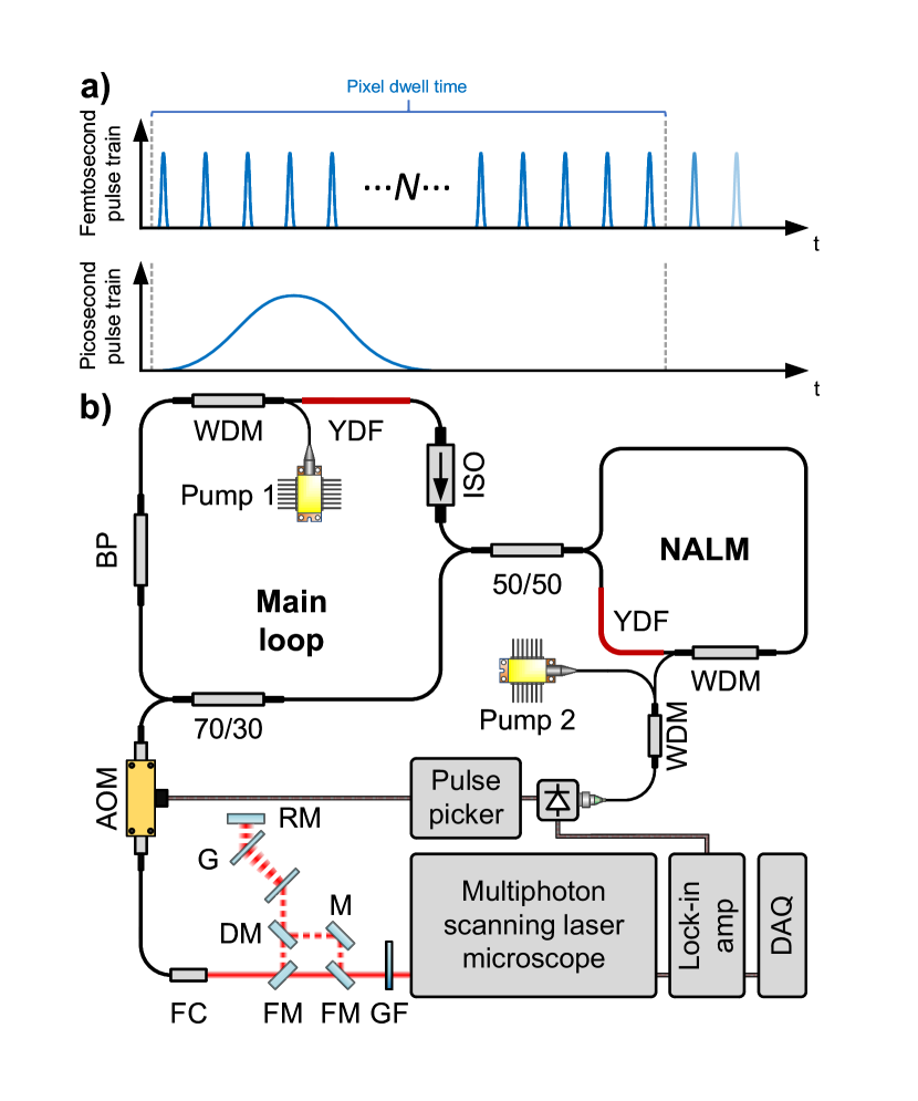
Figure 1: Principle of operation and experimental layout. a) Femtosecond and picosecond pulse trains with the same duty cycle and the same peak power. b) Experimental setup of picosecond fiber laser and multiphoton microscope system. BP – bandpass filter, YDF – Yb-doped fiber, WDM – wavelength-division multiplier, ISO – isolator, AOM – acousto-optic modulator, FC – fiber collimator, FM – flip mirror, DM – D-shaped mirror, G – diffraction grating, RM- retro mirror, M – mirror, GF – gradient index filter, DAQ – data acquisition card.

Here, we experimentally show that an efficient TPE is possible by directly using picosecond pulses with reduced $f_{rep}$. We designed a monolithic, all-polarization-maintaining Yb:fiber laser producing 10 ps pulses with $\sim$10 nJ energy directly at the oscillator output. The laser was connected with a fiber-coupled pulse picker unit and directly applied in multiphoton microscopy without pulse compression. We compared those results with images obtained using a compressed 205 fs pulse train without reducing the $f_{rep}$ (keeping the same duty cycle). We show the advantage of utilizing the picosecond pulse train with pulse picking in two imaging modalities: TPE fluorescence and second harmonic generation (SHG) microscopy. Picosecond excitation is less susceptible to chromatic dispersion of a microscope and less susceptible to pulse compression imperfections, thus making it a preferred solution for endoscopic applications. The omission of the pulse compression unit enables the all-fiber configuration and lowers the setup costs and complexity.

A schematic diagram of the laser system is illustrated in Fig. 1(b). Pulses were first generated by a self-starting Yb:fiber figure-eight laser consisting of two cavity sections: the main loop and the nonlinear amplification loop mirror (NALM) [24], each pumped with a 976 nm laser diode followed by an isolator and a pump protector. The NALM loop comprised a reflection-type wavelength-division multiplexer (WDM) and an asymmetrically placed active Yb-doped fiber (YDF, Coherent PM-YSF-HI-HP). The main loop comprised a YDF, an isolator (ISO), a WDM, a 10-nm bandpass filter (BP), and a fiber coupler, which led 70% of the optical power out of the system. All fibers and components were polarization-maintaining.

To change the $f_{rep}$, the pulse picker unit consisting of an acousto-optic modulator (AOM, G&H Fiber-Q) and an electronic driver (AA Optoelectronic PPKS200) was added to the setup. The modulator can pick out single pulses at a desired $f_{rep}$. The transmission of the pulses was synchronized with the original pulse train supplied to the photodiode (Thorlabs PDA05CF2) from the previously unused port in the WDM. The user can change the $f_{rep}$ of the pulse train by dividing its value by a positive integer. The output beam was collimated (FC, Schäfter+Kirchhoff 60FC-4-A11) and was directed to the custom-built multiphoton scanning laser microscope (described in [25]), working in TPE epi-fluorescence or SHG mode. The photomultiplier tube output (Thorlabs PMT2101) was connected to a lock-in amplifier (Zurich Instruments HF2LI) with a reference frequency from the photodiode. The demodulated signal was sampled with a data acquisition card (DAQ, NI PCIe-6363).

The output laser beam could be directed through a typical Treacy compressor [26] using mirrors on a flip mount. It comprised two parallel transmission diffraction gratings (Coherent LightSmyth, 1000 grooves/mm, G) with an estimated group delay dispersion of -1.17 $ps^{2}$ and transmission of 79%. This way, we could form two types of excitation pulse trains: i) a picosecond pulse train with adjustable $f_{rep}$, and ii) a femtosecond pulse train where, for comparison, we keep the $f_{rep}$ unchanged. Both beams passed through the gradient filter (GF, Thorlabs NDL-10C-4) on their way into the multiphoton microscope, which was introduced to keep the average powers of both beams the same.

The laser was characterized using an optical autocorrelator (APE PulseCheck), SPIDER (Fluence Blueback),

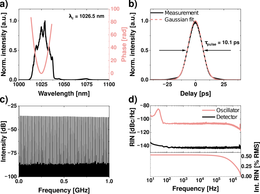
Figure 2: Characterization of the laser directly at the oscillator output. a) The optical spectrum with spectral phase (blue). b) Autocorrelation of the pulse and the Gaussian fit. c) The RF spectrum. d) RIN of the oscillator and corresponding integrated value.

optical spectrum analyzer (Yokogawa AQ6370B), RF spectrum analyzer (Rhode&Schwarz FPL1007), digital oscilloscope (Rhode&Schwarz RTA4004), photodiode (Discovery Semiconductors DSC2-50S), and power meter (Thorlabs PM400) with a thermal sensor (Thorlabs S401C). Relative intensity noise (RIN) was measured using a noise analyzer (Thorlabs PNA1) within the 6 Hz – 3 MHz range and a Thorlabs PDA10CS2 photodetector.

Figure 2 summarizes the laser performance directly at the oscillator output. The oscillator generated pulses at the center wavelength of 1026.5 nm with full width at half-maximum (FWHM) of 15.6 nm [Fig. 2(a)]. The spectrum also consisted of a smaller peak at around 1075 nm (shift of 440 $cm^{-1}$) caused by Raman scattering. We established numerically and experimentally that the peak holds only 1.5% of the average power. The pulse duration was 10.1 ps, assuming a Gaussian pulse shape, as shown in Fig. 2(b). The broad spectrum of harmonics in the RF spectrum [Fig. 2(c)] showed a good stability. The signal-to-noise ratio of the fundamental beat note (at $f_{rep}$ of 15.2 MHz) was equal to 74 dB [see Fig S1(a)]. The oscillator’s RIN measured from 10 Hz to 3 MHz can be seen in Fig. 2(d). The integrated RIN of the oscillator measured in this frequency range was equal to around 0.53% root-mean square (RMS), measured in laboratory conditions, with no thermal stabilization. The output power was equal to 148.5 mW with perfect long-term power stability of 0.05% RMS measured over 3 hours after 1 hour of warm-up [shown in Fig. S1(c)]. This output power value is comparable with state-of-the-art high-power oscillators [27] and ensures enough power is left for the imaging after adding more elements, and excellent power stability guarantees the same average power at each pixel.

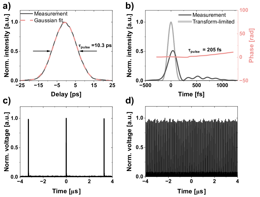
Figure 3: Characterization of two pulse trains used in the experiment. a) Autocorrelation of the pulse after the pulse picker unit with a Gaussian fit. b) Reconstructed temporal profile of the pulse after compression. c) Oscilloscope traces of the picosecond pulse train ($f_{rep}$ = 0.3 MHz). d) Oscilloscope traces of the femtosecond pulse train ($f_{rep}$ = 15.2 MHz).

After propagating through the AOM, there was no significant change in the optical spectrum [see Fig. S3(a)]. Pulse duration [Fig. 3(a)] got slightly longer (10.3 ps) because of propagation in approx. 1.25 m of added fiber. Adding the AOM caused a loss of around 40%, resulting in a pulse energy of 5.6 nJ. Figure 3(b) shows the temporal profile of the pulse after compression. We obtained a FWHM duration of 205 fs with approximately 50% of the peak power of the transform-limited pulse. The optical spectrum was centered at 1029 nm, as shown in Fig. S3(b).

For the experiment, we had to establish the pulse picker’s picking ratio. As shown in Eq. 2 and explained before, we had to maintain the same average power and duty cycle for the picosecond and femtosecond pulse trains. Knowing the FWHM pulse durations of both pulses and the $f_{rep}$ of the oscillator, we could calculate how many times the $f_{rep}$ of the longer pulse should be lowered while maintaining the same duty cycle by:

$$f_{rep2}=\frac{\tau_{p1}\cdot f_{rep1}}{\tau_{p2}},$$ (3)

where $f_{rep1}$, $\tau_{p1}$ correspond to the pulse parameters after compression, and $f_{rep2}$, $\tau_{p2}$ correspond to the pulse received after the pulse picker unit. These calculations established that $f_{rep2}$ should equal 0.3 MHz, corresponding to the picking ratio of 1/50 (resulting in the average power of 1.6 mW). Figures 3(c) and (d) illustrate the difference in $f_{rep}$ values of both pulse trains. The duty cycle in each case was 1.6×$10^{-6}$.

Figures 4(a) and (b) show the results of imaging convallaria majalis root transverse section stained with an acridine orange, a nucleic acid-specific fluorophore. Figures 4(c) and (d) show the results of SHG imaging of urea microcrystals. Both samples were imaged using pico- and femtosecond pulse trains with 0.3 MHz and 15.2 MHz $f_{rep}$, respectively. The dwell time of one pixel was set to 10 µs, and the size of the image was 1024×1024 pixels; in all cases, 50 frames were averaged.

The images received using the picosecond pulse train were brighter and, thus, had better contrast. Figures 4(e) and (f) compare pixel intensity histograms and show a significant shift toward higher voltages for the picosecond pulse train. Using a picosecond pulse train for TPE fluorescence resulted in a 54% higher fluorescence signal,

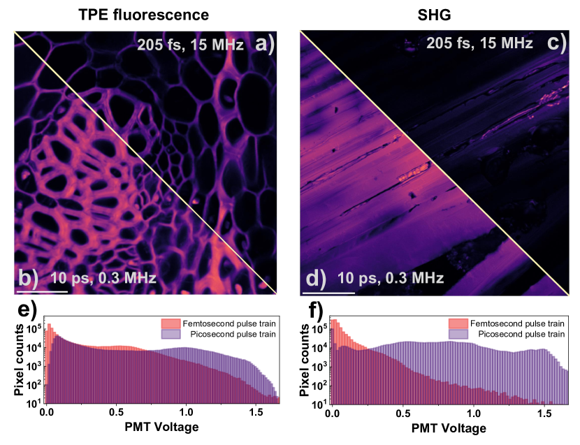
Figure 4: Comparison of imaging with pico- and femtosecond pulse trains. TPE fluorescence images of a stained convallaria majalis sample obtained at 0.7 mW average power using: (a) femtosecond and (b) picosecond pulse trains. Scale bar: 75 $\mu$m. SHG images of urea microcrystals obtained at 0.3 mW average power using (c) femtosecond and (d) picosecond pulse trains. Scale bar: 200 $\mu$m. Histograms of pixel intensity of images of (e) convallaria majalis and (f) urea crystal samples.

while the SHG image had a 90% higher signal. Despite ensuring the same duty cycle and average power for both cases, femtosecond pulses produced fluorescence with lower intensity. We attribute this result to the fact that the femtosecond pulse was not perfectly compressed to its transform limit and to its higher susceptibility to the dispersive effects of the microscope’s inner optics.

To further test the capabilities of our configuration, we searched for a pulse-picking ratio that would result in the same image quality for both cases. We kept constant average power throughout all of our tests, and we could establish that the contrast for both cases was the same when the pulse-picking ratio of 1/14 was used. Figures S4 and S5 show the comparison of both images and corresponding intensity histograms.

Our result shows that efficient multiphoton imaging is possible using picosecond pulses; we have shown that reducing $f_{rep}$ is a very straightforward and effective strategy for improving image quality in two different modalities. Such an approach has several key advantages. Firstly, in the case of chirped pulses typically generated by fiber lasers, it is possible to omit the bulk-optic pulse compressor. This results in a fully-fiberized, maintenance-free portable laser for multiphoton imaging. Secondly, picosecond pulses are significantly less susceptible to chromatic dispersion of microscope optical elements or fiber-based beam delivery systems. We illustrated this issue by numerical simulations (Fig. S6-S8). This makes the proposed laser system a perfect solution for multiphoton endoscopic imaging [15]. Lastly, a significant increase in total fluorescence yield using a lower $f_{rep}$ (>1 $\mu$s temporal pulse separation) has been reported, enabling dark or triplet state relaxation [28]. While generating a low $f_{rep}$ pulse train directly from the oscillator cavity is possible, the pulse picker approach has the added benefit of flexibility. It allows the user to match experimental conditions, such as scanning speed, signal yield, and sample type.

We also note some disadvantages. Firstly, imaging at a lower $f_{rep}$ can be a limiting factor for a fast scanning system; at least one pulse per pixel is needed, ultimately limiting pixel dwell time. Still, imaging with a 1 MHz $f_{rep}$ results in a minimum pixel dwell time of 1 $\mu$s, translating to 3.8 frames per second for a 512×512-pixel image, which is sufficient for most applications. Secondly, this approach requires high pulse energy, which is challenging to produce in fiber lasers without additional amplification. However, pulse energies of >10 nJ can be generated from all-fiber Yb-doped oscillators.

In conclusion, we have demonstrated the benefits of multiphoton microscopy with a high-energy Yb:fiber NALM oscillator with a reduced $f_{rep}$. We have presented that under the same conditions and with the same starting duty cycle, the 205 fs compressed pulse train resulted in worse images than the longer 10 ps pulse train. This setup is all-fiber and portable, and thanks to the pulse-picking unit, its $f_{rep}$ can be adjusted according to one’s needs. The approach is immune to the effect of chromatic dispersion, making it easier to use in real-world conditions. These findings open a new way to use multiphoton microscopy, especially appealing for efficient endoscopic applications.

Funding National Science Centre, Poland (2021/43/D/ST7/01126)

Acknowledgments This research was funded in whole by the National Science Centre (NCN) under grant no. 2021/43/D/ST7/01126. For Open Access, the author has applied a CC-BY public copyright license to any Author Accepted Manuscript (AAM) version arising from this submission. We thank Alicja Kwaśny (WUST) for technical assistance during the construction of the multiphoton microscope and Drs Grazyna Palczewska (University of California Irvine, USA), Łukasz Sterczewski, and Jarosław Sotor (WUST) for inspiring discussions.

Disclosures The authors declare no conflicts of interest.

Data availability Data underlying the results presented in this paper are available in Dataset 1, Ref. [29].

contents

References

- [1] E. E. Hoover and J. A. Squier, \JournalTitleNature Photon pp. 93–101 (2013).
- [2] W. Denk, J. H. Strickler, and W. W. Webb, \JournalTitleScience pp. 73–76 (1990).
- [3] R. S. Pillai, C. Boudoux, G. Labroille, et al., \JournalTitleOpt. Express p. 12741 (2009).
- [4] G. Tsakanova, E. Arakelova, V. Ayvazyan, et al., \JournalTitleBiomed. Opt. Express p. 5834 (2017).
- [5] K. König, K. Schenke-Layland, I. Riemann, and U. A. Stock, \JournalTitleBiomaterials pp. 495–500 (2005).
- [6] A. Rohrbacher, O. E. Olarte, V. Villamaina, et al., \JournalTitleOpt. Express p. 10677 (2017).
- [7] J. Paoli, M. Smedh, A.-M. Wennberg, and M. B. Ericson, \JournalTitleJournal of Investigative Dermatlogy pp. 1248–1255 (2008).
- [8] D. U. Kim, H. Song, W. Song, et al., \JournalTitleOpt. Express p. 12341 (2012).
- [9] B. Chen, T. Jiang, W. Zong, et al., \JournalTitleOpt. Express p. 16544 (2016).
- [10] M. Sun, J. Cui, B. Yu, et al., \JournalTitleOpt. Express p. 24298 (2023).
- [11] D. Stachowiak, J. Bogusławski, A. Głuszek, et al., \JournalTitleBiomed. Opt. Express p. 4431 (2020).
- [12] J. Szczepanek, T. M. Kardaś, M. Michalska, et al., \JournalTitleOpt. Lett. p. 3500 (2015).
- [13] C. Radzewicz, M. J. L. Grone, and J. S. Krasinski, \JournalTitleOptics Communications pp. 185–190 (1996).
- [14] L. Büsing, T. Bonhoff, J. Gottmann, and P. Loosen, \JournalTitleOpt. Express p. 24475 (2013).
- [15] J. C. Jung and M. J. Schnitzer, \JournalTitleOpt. Lett. p. 902 (2003).
- [16] N. G. Horton and C. Xu, \JournalTitleBiomed. Opt. Express p. 1392 (2015).
- [17] J. Pérez-Vizcaíno, O. Mendoza-Yero, G. Mínguez-Vega, et al., \JournalTitleOpt. Lett. p. 440 (2013).
- [18] J. Boguslawski, G. Palczewska, S. Tomczewski, et al., \JournalTitleJournal of Clinical Investigation p. e154218 (2022).
- [19] Y. Liu, H. Tu, and S. A. Boppart, \JournalTitleOpt. Lett. p. 2172 (2012).
- [20] G. A. Murashova, C. A. Mancuso, J. L. Canfield, et al., \JournalTitleBiomed. Opt. Express p. 5228 (2017).
- [21] G. Palczewska, J. Boguslawski, P. Stremplewski, et al., \JournalTitleProc. Natl. Acad. Sci. U.S.A. pp. 22532–22543 (2020).
- [22] S. Karpf, M. Eibl, B. Sauer, et al., \JournalTitleBiomed. Opt. Express p. 2432 (2016).
- [23] J. Song, J. Kang, U. Kang, et al., \JournalTitleSci Rep p. 14244 (2023).
- [24] M. A. Chernysheva, A. A. Krylov, P. G. Kryukov, and E. M. Dianov, \JournalTitleIEEE Photon. Technol. Lett. pp. 1254–1256 (2012).
- [25] J. Bogusławski, A. Kwaśny, D. Stachowiak, and G. Soboń, \JournalTitleOpt. Continuum p. 22 (2024).
- [26] E. Treacy, \JournalTitleIEEE J. Quantum Electron. pp. 454–458 (1969).
- [27] D. Deng, H. Zhang, Q. Gong, et al., \JournalTitleOptics & Laser Technology p. 106010 (2020).
- [28] G. Donnert, C. Eggeling, and S. W. Hell, \JournalTitleNat Methods pp. 81–86 (2007).
- [29] J. Bogusławski, \JournalTitleRepOD V1 (2024). https://doi.org/10.18150/KGUNM5.