High-harmonic generation in semi-Dirac and Weyl semimetals with broken time-reversal symmetry: Exploring merging of Weyl nodes

Abstract

We explore anomalous high-harmonic generation in a model that realizes a transition from a broken time-reversal symmetry Weyl-semimetal to a semi-Dirac regime, i.e. a gapless semimetal with dispersion that is parabolic in one direction and conical in the other two. We point out the intensity of the induced anomalous high harmonics is high in the semi-Dirac regime. For Weyl semimetals, we reveal anomalous high harmonics are due to excitations at momenta where the dispersion is not strictly linear and that in the linearized low-energy theory the anomalous response is harmonic only. Our findings aid experimental characterization of Weyl, Dirac, and semi-Dirac semimetals.

The high harmonic generation (HHG) in condensed matter systems has attracted significant attention due to its potential applications in ultrafast optics (Manzoni et al., 2015; Huttner et al., 2017; Weber et al., 2017; Sie et al., 2019; Nematollahi et al., 2019; Seo et al., 2023; Gao et al., 2020; Boland et al., 2023) and as a characterization method (Cheng et al., 2020; Reinhoffer et al., 2022; Zong et al., 2023; Takasan et al., 2021; Goulielmakis and Brabec, 2022; Li et al., 2020; Murakami et al., 2022; Lv et al., 2021). HHG was proposed to be efficient in Dirac (DSMs) and Weyl semimetals (WSMs) as they are gapless materials with linear energy dispersion (Mikhailov, 2007; Mikhailov and Ziegler, 2008; Lv et al., 2021; Wang et al., 2022; Hafez et al., 2018; Kovalev et al., 2020; Dantas et al., 2021; Germanskiy et al., 2022; Avetissian et al., 2012) and exhibit very high carrier mobilities (Shekhar et al., 2015; Liang et al., 2015; Narayanan et al., 2015; Kumar et al., 2017; Kaneta-Takada et al., 2022). Here we focus on the anomalous optical response (i.e. in the current in a direction perpendicular to the electric field) (Avetissian et al., 2022; Bharti et al., 2022; Wilhelm et al., 2021). In WSMs, the linear anomalous response is proportional to the separation of the Weyl nodes and thus related to topology in these materials. Anomalous high harmonics were proposed as a means for probing the Berry curvature (Silva et al., 2019; Luu and Wörner, 2018; Liu et al., 2017; Yue and Gaarde, 2023). In WSMs, the Berry curvature diverges at the Weyl points (Lv et al., 2021; Nathan et al., 2022) and one might expect this enhances the generation of anomalous high harmonics (although the contribution due to Berry curvature may not be dominant for all driving frequencies (Yue and Gaarde, 2023)).

In WSMs, the band touchings are characterized by their topological charge which determines the chirality of massless Weyl fermions (Armitage et al., 2018) – and by combining two Weyl fermions with opposite chiralities one obtains a Dirac fermion. However, the merging of a pair of Weyl nodes may also give rise to a topologically trivial yet unconventional semi-Dirac regime with parabolic dispersion in the direction of the Weyl nodes separation vector and linear dispersion in the other two directions (i.e. parabolic-2D-conical; see Fig. 1) (Mohanta et al., 2021; Wang et al., 2023). Note that the semi-Dirac regime is distinct from the double-Weyl regime (Fang et al., 2012; Armitage et al., 2018; Bharti and Dixit, 2023) that arises from merging the Weyl nodes with the same chiralities and has parabolic dispersion in two directions. An example of a material that realizes a semi-Dirac regime is $\textrm{SrNbO}_{3}$ where the fourfold degenerate semi-Dirac point is protected by a nonsymmorphic symmetry (Mohanta et al., 2021). Another candidate with such parabolic-2D-conical dispersion, albeit with a tiny energy gap of $6\,\textrm{meV}$, is $\text{ZrTe}_{5}$ (Manzoni et al., 2015; Seo et al., 2023; Martino et al., 2019; Santos-Cottin et al., 2020; Rukelj et al., 2020; Wang and Li, 2020, 2021, 2022; Wang and Cai, 2023; Wang et al., 2023).

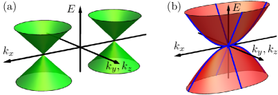
Figure 1: Low energy spectra in (a) Weyl and (b) semi-Dirac semimetals (blue lines highlight the parabolic-2D-conical dispersion).

HHG has already been studied in DSMs and WSMs with broken time-reversal (TRS) (Wilhelm et al., 2021; Avetissian et al., 2022; Bharti et al., 2022) or inversion symmetry (IS) (Liu et al., 2017; Luu and Wörner, 2018; Li et al., 2022). Despite great interest, the qualitative understanding of anomalous HHG (AHHG) in WSMs seems poor, and what aspects of Weyl physics are really contributing is unclear. Here we disentangle the contributions to the response that can be described in terms of well-separated Weyl nodes with conical dispersion (Cano et al., 2017; Vazifeh and Franz, 2013), which was argued to lead to AHHG response that increases with the distance between the nodes (Avetissian et al., 2022), from the contributions that come from non-linearity of dispersion, which becomes large when the nodes approach, and to investigate the effects of the merging of a pair of Weyl nodes to a Dirac or semi-Dirac node.

We consider a minimal 3D model, which describes a transition between two-node WSMs with broken TRS and semi-DSMs with a parabolic-2D-conical energy dispersion. We use the semiconductor Bloch equations (SBE) Floss et al. (2018); Wilhelm et al. (2021); Avetissian et al. (2022); Mrudul and Dixit (2021) to explore the dynamics of the system under the influence of an infrared pulse. We investigate how the anomalous response varies with the separation between the Weyl nodes. In a regime of large Weyl-node separation, we find that whereas the linear response is large, the higher harmonic intensity drops and becomes negligible. Our results reveal the key aspect of AHHG in WSMs: (i) the response vanishes for linearized Weyl dispersion, and hence, (ii) the response arises from deviations from strict linearity. The response becomes large when the Weyl nodes merge and a semi-DSM is realized. We also consider the effects of tilting the Weyl cones. Very recently, a related study has found enhancement of AHHG in multi-Weyl systems (Bharti and Dixit, 2023).

Model and methods — We begin with the Hamiltonian Hasan et al. (2017); Armitage et al. (2018); Bharti et al. (2022) $H(\mathbf{k})=\sum_{i}d_{i}(\mathbf{k})\sigma_{i}$ where $\mathbf{k}=(k_{x},k_{y},k_{z})$ represents the crystal momentum, and Pauli matrices $\sigma_{i}$ act on the pseudospin degree of freedom, such as orbital or sublattice. The components of the vector $\mathbf{d}(\mathbf{k})$ are given by $d_{x}(\mathbf{k})=t_{x}\cos(ak_{x})+t_{y}\cos(bk_{y})+t_{z}\cos(ck_{z})-\gamma$, $d_{y}(\mathbf{k})=t_{y}\sin(bk_{y})$ and $d_{z}(\mathbf{k})=t_{z}\sin(ck_{z})$. The Hamiltonian has orthorhombic symmetry, but for simplicity, we will investigate it for a symmetric choice of parameters $t_{x}=t_{y}=t_{z}=t$ and $a=b=c$ and take dimensionless units $a=1$, $t=1$.

With varying $\gamma$, the Hamiltonian exhibits three distinct regimes, as detailed in the Supplemental Material (SM) S1 (med, ): (a) a trivial insulator phase occurs for $|\gamma|>3$, (b) a WSM phase with one pair of Weyl nodes for $1<|\gamma|<3$, and two pairs of Weyl nodes for $|\gamma|<1$, and (c) at the critical points, $|\gamma|=3$ and $|\gamma|=1$, a semi-Dirac regime arises, featuring one band touching and three band touchings, respectively. In the semi-Dirac regime, the band touchings exhibit a parabolic dispersion along the separation vector of the Weyl nodes ($k_{x}$ direction), while in the perpendicular plane ($k_{y}$–$k_{z}$) they display a 2D conical dispersion. The energy dispersions for the conduction ($c$) and valence ($v$) bands are given by $\epsilon_{c,v}(\mathbf{k})=\pm|\mathbf{d}(\mathbf{k})|$.

The Hamiltonian lacks TRS but possesses IS and mirror symmetry, expressed by $\sigma_{x}H(-\mathbf{k})\sigma_{x}=H(\mathbf{k})$ and $H(k_{x},k_{y},k_{z})=H(-k_{x},k_{y},k_{z})$, respectively. Additionally, Hamiltonians with opposite values of $\gamma$ are related by

$$\sigma_{z}H(\mathbf{R}-\tilde{\mathbf{k}},-\gamma)\sigma_{z}=H(\mathbf{k},\gamma),$$ (1)

where we employed the notation $\tilde{\mathbf{k}}=(k_{x},-k_{y},k_{z})$ and $\mathbf{R}=(\pi,\pi,\pi)$.

At time $t=0$ we expose the system to an ultrashort laser pulse with a duration $T$. Electric field of the laser pulse is described by $\mathbf{E}(t)=E_{0}f_{\tau}\left(t-T/2\right)\sin(\omega_{0}t)\hat{\mathbf{e}}$ where $E_{0}$ is the electric field amplitude, $\hat{\mathbf{e}}$ is the polarization vector (in our calculations we use $\hat{\mathbf{e}}=\hat{e}_{z}$), $\omega_{0}$ is the carrier frequency and $f_{\tau}(t)$ is the Gaussian envelope function $f_{\tau}(t)=\exp\left[-t^{2}/(2\tau^{2})\right]$ where $\tau$ characterizes the pulse width.

The dynamics of the system are described by the SBE for density matrix elements $\rho_{mn}^{\mathbf{k}}$ in the Houston basis Nematollahi et al. (2019); Houston (1940); Krieger and Iafrate (1986):

$$\partial_{t}\rho_{mn}^{\mathbf{k}}(t)=-i\omega_{mn}^{\mathbf{k}(t)}\rho_{mn}^{\mathbf{k}}(t)-\frac{1-\delta_{mn}}{T_{2}}\rho_{mn}^{\mathbf{k}}(t)$$

$$+i\mathbf{E}(t)\cdot\sum_{l}\left[\mathbf{d}_{ln}^{\mathbf{k}(t)}\rho_{ml}^{\mathbf{k}}-\mathbf{d}_{ml}^{\mathbf{k}(t)}\rho_{ln}^{\mathbf{k}}\right]$$ (2)

where we work in units $e_{0}=\hbar=1$, $\mathbf{k}(t)=\mathbf{k}+\mathbf{A}(t)$, $\mathbf{A}(t)=-\int_{0}^{t}\mathbf{E}(t^{\prime})\mathrm{d}t^{\prime}$ is the vector potential, $\omega_{mn}^{\mathbf{k}}=\epsilon_{m}(\mathbf{k})-\epsilon_{n}(\mathbf{k})$ specifies the energy gap, $T_{2}$ is (effective) decoherence time Floss et al. (2018); Kilen et al. (2020); Wilhelm et al. (2021) and $\mathbf{d}_{mn}^{\mathbf{k}}=\langle m,\mathbf{k}|i\partial_{\mathbf{k}}|n,\mathbf{k}\rangle$ are transition dipole moments. Initial condition is $\rho_{mn}(t=0)=\delta_{mv}\delta_{nv}$, i.e. fully occupied valence band.

The current density is

$$\mathbf{J}(t)=\sum_{\mathbf{k}}\mathbf{J}(\mathbf{k},t)=\sum_{\mathbf{k}}\left(-\sum_{m,n}\rho_{mn}^{\mathbf{k}}\mathbf{p}_{nm}^{\mathbf{k}(t)}\right)$$ (3)

where $\mathbf{p}_{nm}^{\mathbf{k}}=\langle n,\mathbf{k}|\partial_{\mathbf{k}}H(\mathbf{k})|m,\mathbf{k}\rangle$ are group-velocity matrix elements. Finally, using the Larmor’s formula Floss et al. (2018), we obtain the spectrum which is proportional to the intensity of emitted radiation:

$$\mathcal{I}(\omega)=\left|\mathcal{FT}\left[\frac{\mathrm{d}}{\mathrm{d}t}\mathbf{J}(t)\right]\right|^{2}=\omega^{2}|\mathbf{J}(\omega)|^{2}.$$ (4)

To obtain a time series of a specific harmonic with $\omega=m\omega_{0}$ ($m\in\mathbb{N}$), we use the following filter:

$$\mathbf{J}^{\omega}(t)=\mathcal{FT}^{-1}\left[\int_{\omega-\delta\omega}^{\omega+\delta\omega}\mathcal{FT}\left[\left(\mathbf{J}(t)\right)\right]\mathrm{d}\omega^{\prime}\right],$$ (5)

where the width of the filter is $2\delta\omega=\omega_{0}$.

We report results for the following values of parameters (taking $a=1$ Å and $t=1$ eV): $\hbar\omega_{0}=0.2$ eV, $E_{0}=0.043$ V/Å, $\tau=40$ fs, $T=790$ fs, $T_{2}=3$ fs. Our choice of parameters follows Ref. (Bharti et al., 2022). We used the discretization of the BZ with $60^{3}$ points.

Results — Excitations at the final time $N_{c}(\mathbf{k},T)=\rho_{cc}(\mathbf{k},T)$, i.e. after the pulse has passed, are shown in Fig. 2 (top). The bottom panels depict dispersions along two high symmetry lines where energy band touchings occur. We see that higher concentrations of excitations coincide with the band touchings where transition dipole moments $\mathbf{d}_{vc}$ diverge Avetissian et al. (2022).

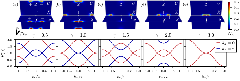
Figure 2: Top: Excitations $N_{c}$ at final time $T$ for different $\gamma$ (increasing from left to right). Excitations occur near band touchings due to the divergence of transition dipole moments. Positive (negative) topological charges are indicated by $+$ ($-$). Bottom: The energy bands are depicted in red and blue colors for momenta along the high symmetry lines $\Gamma$–$X$ ($k_{y}=k_{z}=0$) and $Z$–$U$ ($k_{y}=0$, $k_{z}=\pi$), respectively. For $|\gamma|<1$ there are two pairs of Weyl cones (a); for $\gamma=1$ there are three semi-Dirac points (b); for $1<\gamma<3$ there are two Weyl cones (c,d); and when $\gamma=3$ there is one semi-Dirac point (e). Diagrams are similar for negative $\gamma$ where the roles of $\Gamma$ and $\mathrm{R}$ points of the primitive orthorhombic lattice are reversed which is a consequence of the symmetry (1).

In Fig. 3, we present the $\mathcal{I}_{y}$ component, perpendicular to both the electric field polarization vector and the Weyl node separation vector, for three different values of $\gamma$. We observe that the even harmonics ($\omega=2n\omega_{0}$) vanish due to the IS Boyd and Prato (2008); Bharti et al. (2022). While the spectra may appear similar at first glance, it is important to note that the intensity of higher-order harmonics in the semi-Dirac regimes ($\gamma=1$ and $\gamma=3$) is significantly higher compared to the WSM regime ($\gamma=2$).

To study the dynamics of the semi-Dirac regime in the low-energy limit, i.e. in the case of low frequency and strength of the laser pulse, we compare the lattice result for $\gamma=3$ with the corresponding continuous model obtained by Taylor expansion around the $\Gamma$ point (see SM S1 (med, )). The results, shown in Fig. 3, demonstrate agreement between the two models, confirming that the dominant contributions arise from the region near $\Gamma$ where excitations are present.

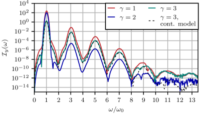
Figure 3: Anomalous spectrum $\mathcal{I}_{y}$ for $\gamma=1$, $2$ and $3$ (corresponding to 3 semi-Dirac nodes, 1 pair of Weyl nodes, and 1 semi-Dirac node, respectively). The dashed line illustrates the continuous model, with the current density integrated over crystal momenta near the $\Gamma$ point within the $\left[-\pi/3,\pi/3\right]^{3}$ range.

From the spectra obtained for different values of $\gamma$ we extract the peak intensities of the odd harmonics, $\omega=(2n+1)\omega_{0}$, and present them in Fig. 4. Intensities show a symmetry $\mathcal{I}_{y}(\gamma)=\mathcal{I}_{y}(-\gamma)$ and also $\mathcal{I}_{y}(\gamma=0)=0$ holds. These observations are a result of IS and symmetry Eq. (1) (for the derivation see SM S2 (med, )). Moreover, we observe a qualitative difference between the first harmonic and higher-order harmonics, where the former increases from $\gamma=0$ to $\gamma=1$ and then decreases from $\gamma=1$ to $\gamma=3$. In contrast, the higher-order harmonics exhibit distinct peaks at $|\gamma|=1$ and $3$ (the reasons underlying the fine structure seen in these peaks are discussed below). The comparatively higher peaks at $\gamma=3$, in comparison to $\gamma=1$, are due to the co-occurrence of three semi-Dirac points, which is related to the symmetric choice $t_{x}=t_{y}=t_{z}$. If hoppings were unequal, the semi-Dirac points would occur at different values of $\gamma$ (SM S1 (med, )), and the present peaks at $\gamma=1$ would split.

To analyze the results presented in Fig. 4, it is beneficial to illustrate the anomalous response decomposed into its harmonic components $J_{y}^{\omega}(t)$ using Eq. (5). Figure 5 displays the outcomes of this decomposition for the first (a) and the third (b–f) harmonic, where we summed the contributions over planes ($k_{y}$–$k_{z}$) perpendicular to the Weyl node separation vector. We will refer to the results of Fig. 5 in the subsequent analysis of AHHG.

The dominant contribution to the first harmonic can be explained by the linear intraband anomalous Hall current Wilhelm et al. (2021); Avetissian et al. (2022); Vampa et al. (2014) which is proportional to the separation between the pairs of Weyl nodes (see Fig. 5a) $J_{y}^{\omega_{0}}(t)\sim\frac{1}{2}\sum_{k}(\mathbf{E}\times\mathcal{B}^{\mathbf{k}(t)})_{y}=\frac{1}{2}E_{z}(t)\frac{1}{(2\pi)^{2}}\int_{-\pi}^{\pi}C_{x}(k_{x})\mathrm{d}k_{x}=-\frac{k_{0}}{4\pi^{2}}E_{z}(t)$ where $\mathcal{B}^{\mathbf{k}}=2i\mathbf{d}_{cv}^{\mathbf{k}}\times\mathbf{d}_{vc}^{\mathbf{k}}$ is the Berry curvature, $C_{x}(k_{x})=\frac{1}{2\pi}\iint(\mathcal{B}^{\mathbf{k}})_{x}\mathrm{d}k_{y}\mathrm{d}k_{z}$ is Chern number for 2D slice at $k_{x}$ and $2k_{0}=2\arccos(\gamma-2)$ is the separation between Weyl nodes for $1<\gamma<3$. When integrating the Chern number over $k_{x}$ we took into account $C_{x}(|k_{x}|<k_{0})=-1$ and $0$ otherwise. Similar reasoning applies for $-1<\gamma<1$, however, in this case, there are two pairs of Weyl nodes (see Fig. 2a) which contribute $C_{x}(|k_{x}|<k_{0})=2$. As a result, in the range $-1<\gamma<1$, the intensity $\mathcal{I}_{y}(\omega=\omega_{0})$ increases twice as fast as it decreases for $1<\gamma<3$ Avetissian et al. (2022). Trivially, the linear anomalous response also goes to zero upon the merger of a pair of Weyl nodes to a Dirac node.

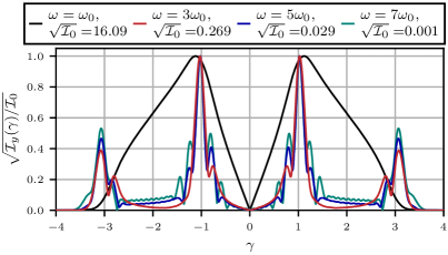
Figure 4: Peak intensities for different $\gamma$ and anomalous harmonics at odd multiples of $\omega_{0}$. For each $\omega$, intensities $\mathcal{I}_{y}(\gamma)$ are scaled by a factor $\mathcal{I}_{0}=\max_{\gamma}\!\left(\mathcal{I}_{y}\right)$.

Understanding the different qualitative behavior of anomalous higher-order harmonics as the Weyl nodes merge, specifically the pronounced peaks at $|\gamma|=1$ and $|\gamma|=3$ in Fig. 4, requires recognizing that high harmonics result from the presence of excitations ($N_{c}$) and interband polarization ($\rho_{vc}$) Avetissian et al. (2022). Consequently, only regions around the Weyl or semi-Dirac points contribute significantly to higher-order harmonics, which implies the response cannot be expressed in terms of $C_{x}(k_{x})$. Furthermore, we have evaluated separately different contributions to the response Avetissian et al. (2022) and found that the Berry curvature contribution and the interband contribution to the high harmonics are of similar magnitude which precludes interpretation of the signal in terms of the Berry curvature alone.

To closely examine the higher-order response, we first consider the case with a pair of well-separated Weyl nodes (foo, ) (Fig. 5b). For each well-separated Weyl node at $\mathbf{k}_{0}$, we can take the region where dispersion is conical and make a Taylor expansion in terms of $\mathbf{q}=\mathbf{k}-\mathbf{k_{0}}$. Then, as detailed in SM S4 (med, ), we have a $C_{2z}$ rotational symmetry with respect to each Weyl node, where the axis is defined by the electric field polarization vector: $\sigma_{z}H(-q_{x},-q_{y},q_{z})\sigma_{z}=H(q_{x},q_{y},q_{z})$, which leads to the relation for the anomalous current:

$${J}_{y}(q_{x},q_{y},q_{z})=-{J}_{y}(-q_{x},-q_{y},q_{z}).$$ (6)

As a result, contributions to the anomalous response near each Weyl node in the linearized limit cancel out (generalization to 3D Dirac cones applies trivially). Hence, the only non-vanishing contribution to AHHG may arise from regions far enough from Weyl nodes, where the linear dispersion approximation no longer applies, but still have non-zero excitations; in other words, a finite response is a result of deviations from strict linearity near each Weyl node . Interestingly, this result applies (under some limitations) even for tilted type-I WSMs (for more details, see SM S5 (med, )). Note that our conclusion regarding the vanishing of anomalous high-harmonic response in the regime of well-separated Weyl cones differs from the one presented in Ref. Avetissian et al. (2022). The resolution of this discrepancy is provided in SM S6 (med, ).

Now, let us consider the case when a pair of Weyl nodes start to approach each other and eventually merge into a semi-Dirac point. Utilizing mirror symmetry $H(k_{x},k_{y},k_{z})=H(-k_{x},k_{y},k_{z})$ (as detailed in SM S7 (med, )), we find

$${J}_{y}(k_{x},k_{y},k_{z})={J}_{y}(-k_{x},k_{y},k_{z}).$$ (7)

Thus, studying only half-space $k_{x}>0$ is sufficient. Bringing a Weyl cone in the proximity of the $\Gamma$ point, e.g. as $\gamma\to 3$, brings along two important changes. Firstly, the density of excitations near $\Gamma$ point starts to increase which leads to increasing contributions to the anomalous current that do not have a counterpart that would cancel them since near $\Gamma$ linear approximation does not hold (Fig. 5c); consequently, the total anomalous current is not vanishing and increases as the Weyl node moves towards $\Gamma$. Secondly, as the Weyl node keeps approaching the $\Gamma$ point, the region near $\Gamma$ with non-linear dispersion and non-zero excitations starts to shrink (Fig. 5d) which first leads to a decrease in the intensity of the anomalous high harmonics; but then as the region near $\Gamma$ keeps shrinking the outer region contributions ($k_{x}>k_{0}$) start to dominate and HHG intensity increases again. This explains the dip near $\gamma=2.9$ observed in Fig. 4. In the limit $\gamma\to 3$ (Fig. 5e) only outer regions ($k_{x}>k_{0}\to 0$) contribute to HHG and since ${J}_{y}(q_{x}=0)=0$ for each Weyl node we have in this limit ${J}_{y}(k_{x}=0)\to 0$. Hence, in the semi-Dirac regime ($\gamma=3$) we still have ${J}_{y}(k_{x})={J}_{y}(-k_{x})$ (from Eq. 7) with additional constraint ${J}_{y}(k_{x}=0)=0$. When the parameter $\gamma$ is increased beyond $3$, the high-harmonic response continues to increase because regions near $k_{x}=0$ also begin to contribute to the overall anomalous current (see Fig. 5f). However, as the gap widens further, the density of excitations quickly decreases, resulting in an overall reduced response in the $\mathcal{I}_{y}$.

We considered a system at half-filling, where the Fermi surface resides at the Weyl points. With small dopings, the validity of our results persists, holding true for both the WSM and semi-Dirac regimes. This is because the regions in the BZ where states in both bands are either empty or occupied do not contribute to the current. For high dopings, the pronounced peaks in Fig. 4 would start to diminish, as regions near $k_{x}=0$ in Fig. 5e would cease to contribute to the AHHG.

Discussion – In conclusion, our study clarifies the distinction between AHHG in WSMs, 3D DSMs, and semi-DSMs. AHHG arises from deviations from the conical dispersion, regardless of the specific (Weyl or Dirac) semimetallic system under consideration. Conversely, in the semi-Dirac regime, the dispersion is quadratic along the Weyl node separation vector, leading to enhanced AHHG. As a result, this distinction provides a valuable opportunity for experimental differentiation between the semi-Dirac and 3D Dirac regimes.

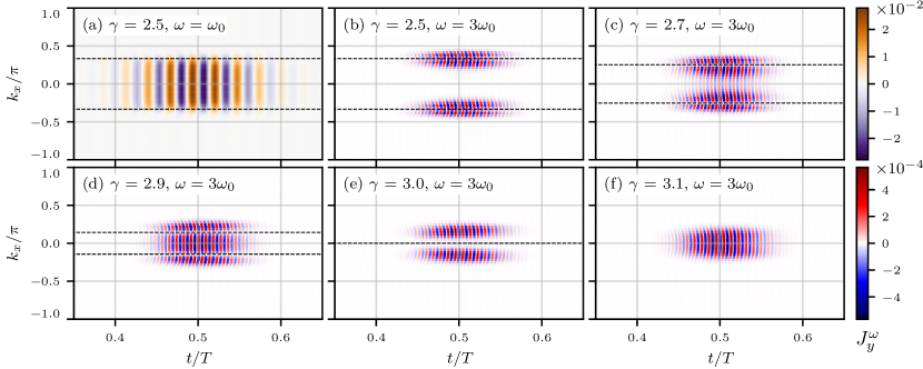
Figure 5: Time series of sliced contributions to the anomalous current ${J}_{y}^{\omega}(t,k_{x})=\sum_{k_{y},k_{z}}{J}_{y}^{\omega}(t,\mathbf{k})$ for (a) the first harmonic, $\omega=\omega_{0}$, and (b–f) the third harmonic, $\omega=3\omega_{0}$, at various $\gamma$ values. Dashed lines indicate the positions of Weyl nodes (a–d) and a semi-Dirac node (e).

We reveal a symmetry that leads to the vanishing of the AHHG in the well-separated Weyl regime and explain enhancement of AHHG (which is maximized near the semi-Dirac regime) in terms of departure from that idealized Weyl situation thereby providing a complementary insight from that offered in a study of multi-Weyl systems (Bharti and Dixit, 2023) that stressed the role of the higher population in the conduction band.

We used a simplified lattice model to study AHHG. In future research, it would be interesting to conduct realistic calculations on $\textrm{SrNbO}_{3}$ (Mohanta et al., 2021) and $\textrm{ZrTe}_{5}$ (Martino et al., 2019; Santos-Cottin et al., 2020; Rukelj et al., 2020). Notably, $\textrm{SrNbO}_{3}$ might be worth investigating, as it hosts symmetry-protected semi-Dirac points at the Brillouin-zone boundary, and applying an external magnetic field generates pairs of Weyl nodes. To generalize our results, it is important to consider the fourfold degeneracy exhibited in such materials. Additionally, investigating similar effects in 2D materials like black phosphorus Kim et al. (2015), which exhibit a mixed quadratic and linear dispersion profile at critical points, would be of interest as well.

It would also be instructive to explore the significance of the over-tilted, type-II Weyl cones on AHHG in our TRS-broken model, which we leave for further studies.

We thank G. Mkrtchian for useful correspondence.

We acknowledge support from the Slovenian Research and Innovation Agency (ARIS) under Contract No. P1-0044; AR was also supported by Grant J2-2514. JM acknowledges support by ARIS under Grant No. J1-2457.

References

- Manzoni et al. (2015) G. Manzoni, A. Sterzi, A. Crepaldi, M. Diego, F. Cilento, M. Zacchigna, P. Bugnon, H. Berger, A. Magrez, M. Grioni, and F. Parmigiani, Phys. Rev. Lett. 115, 207402 (2015).
- Huttner et al. (2017) U. Huttner, M. Kira, and S. W. Koch, Laser & Photonics Reviews 11, 1700049 (2017).
- Weber et al. (2017) C. P. Weber, B. S. Berggren, M. G. Masten, T. C. Ogloza, S. Deckoff-Jones, J. Madéo, M. K. L. Man, K. M. Dani, L. Zhao, G. Chen, J. Liu, Z. Mao, L. M. Schoop, B. V. Lotsch, S. S. P. Parkin, and M. Ali, Journal of Applied Physics 122, 223102 (2017).
- Sie et al. (2019) E. J. Sie, C. M. Nyby, C. D. Pemmaraju, S. J. Park, X. Shen, J. Yang, M. C. Hoffmann, B. K. Ofori-Okai, R. Li, A. H. Reid, S. Weathersby, E. Mannebach, N. Finney, D. Rhodes, D. Chenet, A. Antony, L. Balicas, J. Hone, T. P. Devereaux, T. F. Heinz, X. Wang, and A. M. Lindenberg, Nature 565, 61 (2019).
- Nematollahi et al. (2019) F. Nematollahi, S. A. Oliaei Motlagh, V. Apalkov, and M. I. Stockman, Phys. Rev. B 99, 245409 (2019).
- Seo et al. (2023) S. B. Seo, S. Nah, M. Sajjad, J. Song, N. Singh, S. H. Suk, H. Baik, S. Kim, G.-J. Kim, J.-I. Kim, and S. Sim, Advanced Optical Materials 11, 2201544 (2023).
- Gao et al. (2020) Y. Gao, S. Kaushik, E. J. Philip, Z. Li, Y. Qin, Y. P. Liu, W. L. Zhang, Y. L. Su, X. Chen, H. Weng, D. E. Kharzeev, M. K. Liu, and J. Qi, Nature Communications 11, 720 (2020).
- Boland et al. (2023) J. L. Boland, D. A. Damry, C. Q. Xia, P. Schönherr, D. Prabhakaran, L. M. Herz, T. Hesjedal, and M. B. Johnston, ACS Photonics, ACS Photonics 10, 1473 (2023).
- Cheng et al. (2020) B. Cheng, N. Kanda, T. N. Ikeda, T. Matsuda, P. Xia, T. Schumann, S. Stemmer, J. Itatani, N. P. Armitage, and R. Matsunaga, Phys. Rev. Lett. 124, 117402 (2020).
- Reinhoffer et al. (2022) C. Reinhoffer, P. Pilch, A. Reinold, P. Derendorf, S. Kovalev, J.-C. Deinert, I. Ilyakov, A. Ponomaryov, M. Chen, T.-Q. Xu, Y. Wang, Z.-Z. Gan, D.-S. Wu, J.-L. Luo, S. Germanskiy, E. A. Mashkovich, P. H. M. van Loosdrecht, I. M. Eremin, and Z. Wang, Phys. Rev. B 106, 214514 (2022).
- Zong et al. (2023) A. Zong, B. R. Nebgen, S.-C. Lin, J. A. Spies, and M. Zuerch, Nature Reviews Materials 8, 224 (2023).
- Takasan et al. (2021) K. Takasan, T. Morimoto, J. Orenstein, and J. E. Moore, Phys. Rev. B 104, L161202 (2021).
- Goulielmakis and Brabec (2022) E. Goulielmakis and T. Brabec, Nature Photonics 16, 411 (2022).
- Li et al. (2020) J. Li, J. Lu, A. Chew, S. Han, J. Li, Y. Wu, H. Wang, S. Ghimire, and Z. Chang, Nature Communications 11, 2748 (2020).
- Murakami et al. (2022) Y. Murakami, K. Uchida, A. Koga, K. Tanaka, and P. Werner, Phys. Rev. Lett. 129, 157401 (2022).
- Lv et al. (2021) Y.-Y. Lv, J. Xu, S. Han, C. Zhang, Y. Han, J. Zhou, S.-H. Yao, X.-P. Liu, M.-H. Lu, H. Weng, Z. Xie, Y. B. Chen, J. Hu, Y.-F. Chen, and S. Zhu, Nature Communications 12, 6437 (2021).
- Mikhailov (2007) S. A. Mikhailov, Europhysics Letters 79, 27002 (2007).
- Mikhailov and Ziegler (2008) S. A. Mikhailov and K. Ziegler, Journal of Physics: Condensed Matter 20, 384204 (2008).
- Wang et al. (2022) L. Wang, J. Lim, and L. J. Wong, Laser & Photonics Reviews 16, 2100279 (2022).
- Hafez et al. (2018) H. A. Hafez, S. Kovalev, J.-C. Deinert, Z. Mics, B. Green, N. Awari, M. Chen, S. Germanskiy, U. Lehnert, J. Teichert, Z. Wang, K.-J. Tielrooij, Z. Liu, Z. Chen, A. Narita, K. Müllen, M. Bonn, M. Gensch, and D. Turchinovich, Nature 561, 507 (2018).
- Kovalev et al. (2020) S. Kovalev, R. M. A. Dantas, S. Germanskiy, J.-C. Deinert, B. Green, I. Ilyakov, N. Awari, M. Chen, M. Bawatna, J. Ling, F. Xiu, P. H. M. van Loosdrecht, P. Surówka, T. Oka, and Z. Wang, Nature Communications 11, 2451 (2020).
- Dantas et al. (2021) R. M. A. Dantas, Z. Wang, P. Surówka, and T. Oka, Phys. Rev. B 103, L201105 (2021).
- Germanskiy et al. (2022) S. Germanskiy, R. M. A. Dantas, S. Kovalev, C. Reinhoffer, E. A. Mashkovich, P. H. M. van Loosdrecht, Y. Yang, F. Xiu, P. Surówka, R. Moessner, T. Oka, and Z. Wang, Phys. Rev. B 106, L081127 (2022).
- Avetissian et al. (2012) H. K. Avetissian, A. K. Avetissian, G. F. Mkrtchian, and K. V. Sedrakian, Phys. Rev. B 85, 115443 (2012).
- Shekhar et al. (2015) C. Shekhar, A. K. Nayak, Y. Sun, M. Schmidt, M. Nicklas, I. Leermakers, U. Zeitler, Y. Skourski, J. Wosnitza, Z. Liu, Y. Chen, W. Schnelle, H. Borrmann, Y. Grin, C. Felser, and B. Yan, Nature Physics 11, 645 (2015).
- Liang et al. (2015) T. Liang, Q. Gibson, M. N. Ali, M. Liu, R. J. Cava, and N. P. Ong, Nature Materials 14, 280 (2015).
- Narayanan et al. (2015) A. Narayanan, M. D. Watson, S. F. Blake, N. Bruyant, L. Drigo, Y. L. Chen, D. Prabhakaran, B. Yan, C. Felser, T. Kong, P. C. Canfield, and A. I. Coldea, Phys. Rev. Lett. 114, 117201 (2015).
- Kumar et al. (2017) N. Kumar, Y. Sun, N. Xu, K. Manna, M. Yao, V. Süss, I. Leermakers, O. Young, T. Förster, M. Schmidt, H. Borrmann, B. Yan, U. Zeitler, M. Shi, C. Felser, and C. Shekhar, Nature Communications 8, 1642 (2017).
- Kaneta-Takada et al. (2022) S. Kaneta-Takada, Y. K. Wakabayashi, Y. Krockenberger, T. Nomura, Y. Kohama, S. A. Nikolaev, H. Das, H. Irie, K. Takiguchi, S. Ohya, M. Tanaka, Y. Taniyasu, and H. Yamamoto, npj Quantum Materials 7, 102 (2022).
- Avetissian et al. (2022) H. K. Avetissian, V. N. Avetisyan, B. R. Avchyan, and G. F. Mkrtchian, Phys. Rev. A 106, 033107 (2022).
- Bharti et al. (2022) A. Bharti, M. S. Mrudul, and G. Dixit, Phys. Rev. B 105, 155140 (2022).
- Wilhelm et al. (2021) J. Wilhelm, P. Grössing, A. Seith, J. Crewse, M. Nitsch, L. Weigl, C. Schmid, and F. Evers, Phys. Rev. B 103, 125419 (2021).
- Silva et al. (2019) R. E. F. Silva, Á. Jiménez-Galán, B. Amorim, O. Smirnova, and M. Ivanov, Nature Photonics 13, 849 (2019).
- Luu and Wörner (2018) T. T. Luu and H. J. Wörner, Nature Communications 9, 916 (2018).
- Liu et al. (2017) H. Liu, Y. Li, Y. S. You, S. Ghimire, T. F. Heinz, and D. A. Reis, Nature Physics 13, 262 (2017).
- Yue and Gaarde (2023) L. Yue and M. B. Gaarde, Phys. Rev. Lett. 130, 166903 (2023).
- Nathan et al. (2022) F. Nathan, I. Martin, and G. Refael, Phys. Rev. Res. 4, 043060 (2022).
- Armitage et al. (2018) N. P. Armitage, E. J. Mele, and A. Vishwanath, Rev. Mod. Phys. 90, 015001 (2018).
- Mohanta et al. (2021) N. Mohanta, J. M. Ok, J. Zhang, H. Miao, E. Dagotto, H. N. Lee, and S. Okamoto, Phys. Rev. B 104, 235121 (2021).
- Wang et al. (2023) J.-R. Wang, W. Li, and C.-J. Zhang, Phys. Rev. B 107, 155125 (2023).
- Fang et al. (2012) C. Fang, M. J. Gilbert, X. Dai, and B. A. Bernevig, Phys. Rev. Lett. 108, 266802 (2012).
- Bharti and Dixit (2023) A. Bharti and G. Dixit, Phys. Rev. B 107, 224308 (2023).
- Martino et al. (2019) E. Martino, I. Crassee, G. Eguchi, D. Santos-Cottin, R. D. Zhong, G. D. Gu, H. Berger, Z. Rukelj, M. Orlita, C. C. Homes, and A. Akrap, Phys. Rev. Lett. 122, 217402 (2019).
- Santos-Cottin et al. (2020) D. Santos-Cottin, M. Padlewski, E. Martino, S. B. David, F. Le Mardelé, F. Capitani, F. Borondics, M. D. Bachmann, C. Putzke, P. J. W. Moll, R. D. Zhong, G. D. Gu, H. Berger, M. Orlita, C. C. Homes, Z. Rukelj, and A. Akrap, Phys. Rev. B 101, 125205 (2020).
- Rukelj et al. (2020) Z. Rukelj, C. C. Homes, M. Orlita, and A. Akrap, Phys. Rev. B 102, 125201 (2020).
- Wang and Li (2020) Y.-X. Wang and F. Li, Phys. Rev. B 101, 195201 (2020).
- Wang and Li (2021) Y.-X. Wang and F. Li, Phys. Rev. B 103, 115202 (2021).
- Wang and Li (2022) Y.-X. Wang and F. Li, Phys. Rev. B 106, 205102 (2022).
- Wang and Cai (2023) Y.-X. Wang and Z. Cai, Phys. Rev. B 107, 125203 (2023).
- Li et al. (2022) Z.-Y. Li, Q. Li, and Z. Li, Chinese Physics B 31, 124204 (2022).
- Cano et al. (2017) J. Cano, B. Bradlyn, Z. Wang, M. Hirschberger, N. P. Ong, and B. A. Bernevig, Phys. Rev. B 95, 161306 (2017).
- Vazifeh and Franz (2013) M. M. Vazifeh and M. Franz, Phys. Rev. Lett. 111, 027201 (2013).
- Floss et al. (2018) I. Floss, C. Lemell, G. Wachter, V. Smejkal, S. A. Sato, X.-M. Tong, K. Yabana, and J. Burgdörfer, Phys. Rev. A 97, 011401 (2018).
- Mrudul and Dixit (2021) M. S. Mrudul and G. Dixit, Phys. Rev. B 103, 094308 (2021).
- Hasan et al. (2017) M. Z. Hasan, S.-Y. Xu, I. Belopolski, and S.-M. Huang, Annual Review of Condensed Matter Physics 8, 289 (2017).
- (56) See Supplemental Material for more details.
- Houston (1940) W. V. Houston, Phys. Rev. 57, 184 (1940).
- Krieger and Iafrate (1986) J. B. Krieger and G. J. Iafrate, Phys. Rev. B 33, 5494 (1986).
- Kilen et al. (2020) I. Kilen, M. Kolesik, J. Hader, J. V. Moloney, U. Huttner, M. K. Hagen, and S. W. Koch, Phys. Rev. Lett. 125, 083901 (2020).
- Boyd and Prato (2008) R. Boyd and D. Prato, Nonlinear Optics (Elsevier Science, 2008).
- Vampa et al. (2014) G. Vampa, C. R. McDonald, G. Orlando, D. D. Klug, P. B. Corkum, and T. Brabec, Phys. Rev. Lett. 113, 073901 (2014).
- (62) We define well-separated Weyl nodes as those for which the energy gap in the region between the nodes becomes significantly larger than the electric-field induced perturbation () in the SBE (High-harmonic generation in semi-Dirac and Weyl semimetals with broken time-reversal symmetry: Exploring merging of Weyl nodes). Additionally, as shown in SM S3 (med, ), should be small in comparison to . These two conditions ensure that contributions to the anomalous current remain localized near each Weyl node, allowing the nodes to be treated separately.
- Note (1) In a different setting, unrelated to HHG, the importance of deviations from strict linearity was discussed in Ref. (Bharti et al., 2023).
- Kim et al. (2015) J. Kim, S. S. Baik, S. H. Ryu, Y. Sohn, S. Park, B.-G. Park, J. Denlinger, Y. Yi, H. J. Choi, and K. S. Kim, Science 349, 723 (2015).
- Bharti et al. (2023) A. Bharti, M. Ivanov, and G. Dixit, Phys. Rev. B 108, L020305 (2023).