Fast Rates in Online Convex Optimization
by Exploiting the Curvature of Feasible Sets

Abstract

In this paper, we explore online convex optimization (OCO) and introduce a new analysis that provides fast rates by exploiting the curvature of feasible sets. In online linear optimization, it is known that if the average gradient of loss functions is larger than a certain value, the curvature of feasible sets can be exploited by the follow-the-leader (FTL) algorithm to achieve a logarithmic regret. This paper reveals that algorithms adaptive to the curvature of loss functions can also leverage the curvature of feasible sets. We first prove that if an optimal decision is on the boundary of a feasible set and the gradient of an underlying loss function is non-zero, then the algorithm achieves a regret upper bound of $O(\rho\ln T)$ in stochastic environments. Here, $\rho>0$ is the radius of the smallest sphere that includes the optimal decision and encloses the feasible set. Our approach, unlike existing ones, can work directly with convex loss functions, exploiting the curvature of loss functions simultaneously, and can achieve the logarithmic regret only with a local property of feasible sets. Additionally, it achieves an $O(\sqrt{T})$ regret even in adversarial environments where FTL suffers an $\Omega(T)$ regret, and attains an $O(\rho\ln T+\sqrt{C\rho\ln T})$ regret bound in corrupted stochastic environments with corruption level $C$. Furthermore, by extending our analysis, we establish a regret upper bound of $O\Big{(}T^{\frac{q-2}{2(q-1)}}(\ln T)^{\frac{q}{2(q-1)}}\Big{)}$ for $q$-uniformly convex feasible sets, where uniformly convex sets include strongly convex sets and $\ell_{p}$-balls for $p\in[1,\infty)$. This bound bridges the gap between the $O(\ln T)$ regret bound for strongly convex sets ($q=2$) and the $O(\sqrt{T})$ regret bound for non-curved sets ($q\to\infty$).

1 Introduction

This paper considers online convex optimization (OCO), a framework in which a learner and environment interact in a sequential manner. At the beginning, a convex body (or feasible set) $K\subset\mathbb{R}^{d}$ is given. At each round $t\in[T]\coloneqq\{1,\dots,T\}$, the learner selects a decision $x_{t}\in K$ from the convex body $K$ using information obtained up to round $t-1$. Then, the environment determines a convex loss function $f_{t}\colon K\to\mathbb{R}$, and the learner suffers loss $f_{t}(x_{t})$ and observes $\nabla f_{t}(x_{t})\in\mathbb{R}^{d}$. The goal of the learner is to minimize the regret, which is defined as the expectation of the difference between the cumulative loss of decisions chosen by the learner and that of a single optimal decision fixed in hindsight, that is, $\mathsf{R}_{T}=\max_{x\in K}\mathbb{E}{\left[\sum_{t=1}^{T}\left(f_{t}(x_{t})-f_{t}(x)\right)\right]}\,.$ The optimal decision is defined as $x_{\star}=\operatorname*{arg\,min}_{x\in K}\mathbb{E}{\left[\sum_{t=1}^{T}f_{t}(x)\right]}$. This problem is called online linear optimization (OLO) when loss function $f_{t}$ is a linear function, i.e., $f_{t}(\cdot)=\langle g_{t},\cdot\rangle$ for some $g_{t}\in\mathbb{R}^{d}$.

In OCO and OLO, it is known that under Lipschitz continuous $f_{t}$, the well-known online gradient descent (OGD) achieves an $O(\sqrt{T})$ regret upper bound (Zinkevich, 2003). In general, this upper bound cannot be improved and is known to match the $\Omega(\sqrt{T})$ regret lower bound (Hazan et al., 2007). However, this lower bound can be circumvented under certain conditions. The most typical example is by exploiting the curvature of loss functions. It is known that OGD with a learning rate of $\Theta(1/t)$ and online Newton step (ONS) can achieve an $O(\frac{1}{\alpha}\ln T)$ and $O(\frac{d}{\beta}\ln T)$ regret for $\alpha$-strongly-convex and $\beta$-exp-concave loss functions, respectively (Hazan et al., 2007).

Another way to circumvent the lower bound is to harness the curvature of feasible set $K$. Existing studies have shown that in OLO if the feasible set is curved and loss vectors $g_{t}$ are biased towards a specific direction, the follow-the-leader (FTL) algorithm can achieve a logarithmic regret. Huang et al. (2017) is the first investigation, proving that under the growth condition that there exists $L>0$ such that $\|g_{1}+\cdots+g_{t}\|_{2}\geq tL$ for any $t\in[T]$, FTL achieves an $O(\frac{G^{2}}{\lambda L}\ln T)$ regret for $\lambda$-strongly convex $K$ and $G$-Lipschitz loss functions. This bound matches their lower bound of $\Omega(\frac{1}{\lambda L}\ln T)$. Molinaro (2022) also proves that FTL can achieve a logarithmic regret under the different assumption on the loss vectors that $g_{t}\leq 0$ for all $t\in[T]$, providing an intuitive and simple proof.

Their approach, however, has several remaining limitations. The first limitation is that they only consider OLO. While the linearization technique allows us to solve OCO by OLO, this prevents us from leveraging the curvature of loss functions. The second limitation is that their approach may suffer an $\Omega(T)$ regret if the ideal conditions on loss vectors, such as the growth condition, are not satisfied. Note that we cannot know in advance whether such conditions are satisfied or not. The third limitation is that their analysis requires the curvature over the entire boundary of the feasible set, which is a rather limited condition.

To overcome these limitations, we consider using algorithms adaptive to the curvature of loss functions (van Erven and Koolen, 2016; van Erven et al., 2021; Wang et al., 2020), also known as universal online learning. The original motivation of this line of work is to automatically achieve a regret bound that depends on the true curvature level of loss functions, e.g., parameters of strong convexity or exp-concavity, without knowing them. The crux for achieving this adaptivity is to derive a bound of $\sum_{t=1}^{T}\langle\nabla f_{t}(x_{t}),x_{t}-x_{\star}\rangle=O(c_{\mathsf{sc}}\sqrt{\sum_{t=1}^{T}\|x_{t}-x_{\star}\|_{2}^{2}\ln T})$ for some $c_{\mathsf{sc}}>0$.

Table 1: Comparison of our regret upper bounds with existing bounds. All bounds presented here assume that loss functions are $G$-Lipschitz (except Lines 1–3) and $x_{\star}$ is on the boundary of $K$. The upper bounds that contain the variable $L>0$ assume $\|g_{1}+\cdots+g_{t}\|_{2}\geq tL$ for all $t\in[T]$. Here, $f^{\circ}=\mathbb{E}_{f\sim\mathcal{D}}{\left[f\right]}$, $C\geq 0$ is the corruption level, and the $\widetilde{\Omega}$ notation ignores logarithmic factors. Note that regret upper bounds proven in this work can be simultaneously achieved by the same algorithm with identical parameters. Note that $(\kappa,2)$-uniformly convex set is $\kappa$-strongly convex. Here, Huang et al. (2017) is abbreviated as H+17, Theorem as Thm, Corollary as Cor, and sphere-enclosed as sphere-enc.

Reference	Feasible set	Loss functions	Regret bound
H+17, This work (Thm 6)	ellipsoid $W_{\lambda}$ in (2) ($\lambda$-strongly convex)	$f_{t}(\cdot)=\langle h_{t}^{L},\cdot\rangle$ in Thm 4	$\displaystyle\Omega\left(\frac{1}{\lambda L}\ln T\right)$,  $\displaystyle\Omega\left(\frac{1}{\lambda\|\nabla f^{\circ}(x_{\star})\|_{2}}\ln T\right)$
This work (Thm 7)		corrupted	$\displaystyle\widetilde{\Omega}\left(\frac{1}{\lambda\|\nabla f^{\circ}(x_{\star})\|_{2}}+\sqrt{\frac{C}{\lambda\|\nabla f^{\circ}(x_{\star})\|_{2}}}\right)$
This work (Cor 11)		$f_{t}(\cdot)=\langle h_{t}^{L},\cdot\rangle$ in Thm 4	$\displaystyle O\left(\frac{1}{\lambda L}\ln T\right)$
This work (Thms 9, 13)	$(\rho,x_{\star},f^{\circ})$-sphere-enclosed	stochastic, convex	$\displaystyle O\left(\frac{G^{2}\rho}{\|\nabla f^{\circ}(x_{\star})\|}_{2}\ln T\right)$
This work (Thm 12)	$(\rho,\widetilde{x}_{\star},\widetilde{f}^{\circ})$-sphere-enc.	corrupted, convex	$\displaystyle O\left(\frac{G^{2}\rho}{\|\nabla\widetilde{f}^{\circ}(\widetilde{x}_{\star})\|}_{2}\ln T+\sqrt{\frac{CG^{2}\rho}{\|\nabla\widetilde{f}^{\circ}(\widetilde{x}_{\star})\|}_{2}\ln T}\right)$
Huang et al. (2017)	$\lambda$-strongly convex	adversarial, linear	$\displaystyle O\left(\frac{G^{2}}{\lambda L}\ln T\right)$
Molinaro (2022)		adversarial, linear	$\displaystyle O\left(\frac{G\,c_{\|\cdot\|}}{\lambda}\ln T\right)$ $\left(c_{\|\cdot\|}=\max_{x\in\mathbb{R}_{+}^{d}\colon\|x\|=1}\langle u,x\rangle\right)$
This work (Thm 15)		stochastic, convex	$\displaystyle O\left(\frac{G^{2}}{\lambda\|\nabla f^{\circ}(x_{\star})\|_{\star}}\ln T\right)$
Kerdreux et al. (2021a)	$(\kappa,q)$-uniformly convex	adversarial, linear	$\displaystyle O\left(\frac{G^{\frac{q}{q-1}}}{\left(\kappa L\right)^{\frac{1}{q-1}}}T^{\frac{q-2}{q-1}}\right)$
This work (Thm 15)		stochastic, convex	$\displaystyle O\left(\frac{G^{\frac{q}{q-1}}}{\left(\kappa\|\nabla f^{\circ}(x_{\star})\|_{\star}\right)^{\frac{1}{q-1}}}T^{\frac{q-2}{2(q-1)}}\left(\ln T\right)^{\frac{q}{2(q-1)}}\right)$

1.1 Contributions of This Paper

In this paper, we first show that algorithms with the universal online learning guarantee can exploit the curvature of feasible sets and overcome the three limitations mentioned earlier. The informal statement is as follows.

Theorem 1 (informal version of Theorems 9 and 12).

Consider online convex optimization over convex body $K$. Then, any algorithm with $\sum_{t=1}^{T}\langle\nabla f_{t}(x_{t}),x_{t}-x_{\star}\rangle=O(c_{\mathsf{sc}}\sqrt{\sum_{t=1}^{T}\|x_{t}-x_{\star}\|_{2}^{2}\ln T})$ for some $c_{\mathsf{sc}}>0$ achieves the following regret bound in stochastic environments:

$$\mathsf{R}_{T}=O\left(\frac{c_{\mathsf{sc}}^{2}\,\rho}{\|\nabla f^{\circ}(x_{\star})\|_{2}}\ln T\right)\,,$$ (1)

where $f^{\circ}=\mathbb{E}_{f_{t}\sim\mathcal{D}}{\left[f_{t}\right]}$ and $\rho>0$ is the smallest radius of a sphere that includes $x_{\star}$, encloses $K$, and is such that $\nabla f^{\circ}(x_{\star})$ points towards the center of the sphere. The same algorithm achieves $\mathsf{R}_{T}=O(\rho\ln T+\sqrt{C\rho\ln T})$ in corrupted stochastic environments with corruption level $C\geq 0$ and achieves $\mathsf{R}_{T}=O(\sqrt{T})$ in adversarial environments.

This regret upper bound matches an existing lower bound in Huang et al. (2017, Theorem 9), specifically when considering the environment employed to construct the lower bound. This will be formally stated in Corollary 11.

The advantage of our approach over existing approaches is that it overcomes all three limitations of the existing approach mentioned earlier. That is, (i) in contrast to existing studies, it can work with OCO without the linearization, allowing us to simultaneously exploit the curvature of feasible sets and the curvature of loss functions (see Theorem 13). (ii) Even if the specific conditions on loss vectors, such as the growth condition, are not satisfied, an $O(\sqrt{T})$ regret upper bound can be achieved in the worst-case. (iii) The local structure of $K$ around optimal decision $x_{\star}$ is sufficient for the algorithm to achieve the logarithmic regret. As a further advantage, the approach can achieve an $O(\rho\ln T+\sqrt{C\rho\ln T})$ regret bound for corrupted stochastic environments with corruption level $C\geq 0$, which are intermediate environments between stochastic and adversarial environments (Theorem 12). We provide a regret lower bound that nearly matches this upper bound (Theorem 7).

The proposed approach can be further extended to obtain fast rates on uniformly convex feasible sets, a broader class that includes strongly convex sets and $\ell_{p}$-ball for $p\in[1,\infty)$. For $q$-uniformly convex $K$, Kerdreux et al. (2021a) prove an $O\big{(}T^{\frac{q-2}{q-1}}\big{)}$ regret upper bound, which becomes smaller than $O(\sqrt{T})$ only when $q\in(2,3)$. We successfully improve this regret bound by proving an $O\big{(}T^{\frac{q-2}{2(q-1)}}\left(\ln T\right)^{\frac{q}{2(q-1)}}\big{)}$ regret bound, which is fast rates for all $q>2$ and is strictly better than the bound by Kerdreux et al. (2021a). Interestingly, our regret bound interpolates between the $O(\ln T)$ bound for strongly convex sets (when $q=2$) and the $O(\sqrt{T})$ bound for non-curved feasible sets (when $q\to\infty$). Table 1 summarizes the regret comparison against existing studies.

1.2 Additional Related Work

Fast rates on strongly or uniformly convex sets

Exploiting the curvature of feasible sets has been considered in OLO. In addition to the previously discussed studies (Huang et al., 2017; Molinaro, 2022; Kerdreux et al., 2021a), in online learning with a hint, where a context $m_{t}$ satisfying $m_{t}^{\top}x_{t}\geq c\|x_{t}\|_{2}^{2}$ is given every round, we can achieve an $O(\frac{1}{c}\ln T)$ regret (Dekel et al., 2017). The curvature was also exploited for reducing the number of linear optimization oracle calls in constructing Frank-Wolfe-based algorithms (Mhammedi, 2022). Beyond the scope of online learning, exploiting the curvature of feasible sets has been investigated also in offline optimization, where the goal is to solve $\min_{x\in K}f(x)$ for a given smooth convex function $f$ (Levitin and Polyak, 1966; Demyanov and Rubinov, 1970; Dunn, 1979; Garber and Hazan, 2015; Kerdreux et al., 2021a).

Fast rates on curved loss functions

One classical and seminal work to exploit the curvature of loss functions is by Hazan et al. (2007). Our approach is based on the results of universal online learning, the motivation of which is to be adaptive to parameters of loss curvature without knowing them. This line of investigation was initiated by van Erven and Koolen (2016); van Erven et al. (2021), who establish an algorithm, MetaGrad, that achieves an $O(\frac{d}{\beta}\ln T)$ regret bound if loss functions are $\beta$-exp-concave and an $O(\sqrt{T\ln\ln T})$ bound otherwise, without knowing the curvature of loss functions. The underlying idea is to run several experts in parallel with different curvature parameters, and then another expert algorithm integrates their results to choose decisions. This algorithm was later extended to achieve an $O(\frac{1}{\alpha}\ln T)$ regret bound when the loss functions are $\alpha$-strongly convex (Wang et al., 2020). Roughly speaking, this was made possible by considering MetaGrad with additional experts of OGD with a learning rate of $\Theta(1/t)$. They provided a bound of $\sum_{t=1}^{T}\langle\nabla f_{t}(x_{t}),x_{t}-x_{\star}\rangle=O(G\sqrt{\sum_{t=1}^{T}\|x_{t}-x_{\star}\|_{2}^{2}\ln T}+GD\ln T)$ for $D=\max_{x,y\in K}\|x-y\|_{2}$. This universal online learning framework has been extended to a simpler form (Zhang et al., 2022) and to a form with the path-length bound (Yan et al., 2023). It is worth noting that these algorithms are efficient since the number of experts is at most $O(\ln T)$.

Intermediate environments in OCO

The corrupted stochastic environments considered in this paper are similar to the formulations investigated in the context of expert problems and multi-armed bandit problems (Lykouris et al., 2018; Ito, 2021), and this environment is also referred to as stochastic environments with adversarial corruptions. Sachs et al. (2022, 2023) considered a more general environment, the stochastically extended adversary (SEA) model. It would be important future work to extend our results to the SEA model. Note that they do not consider the curvature of feasible sets.

2 Preliminaries

Let $e_{i}\in\{0,1\}^{d}$ be the $i$-th standard basis of $\mathbb{R}^{d}$, and $\mathbf{1}$ be the all-one vector. For $p\in[1,\infty]$ and vector $x$, let $\|x\|_{p}$ be $\ell_{p}$-norm. Let $\xi>0$ be a constant satisfying $\|x\|_{2}\leq\xi\|x\|$ for any $x\in\mathbb{R}^{d}$. For a norm $\|\cdot\|$, we use $\|x\|_{\star}=\sup\{\langle x,y\rangle\colon\|y\|\leq 1\}$ to denote its dual norm. Let $\mathbb{B}_{\|\cdot\|}(x,r)$ be a ball with a radius $r$ centered at $x$ associated with a norm $\|\cdot\|$, i.e., $\mathbb{B}_{\|\cdot\|}(x,r)=\left\{z\colon\|z-x\|\leq r\right\}$. We write $\mathbb{B}(x,r)$ to denote the Euclidean ball with radius $r$ centered at $x$ and $\mathbb{B}_{\|\cdot\|}$to denote the unit ball. For convex body $K$, let $\operatorname{bd}(K)$ be the boundary of $K$. A function $f\colon\mathbb{R}^{d}\to(-\infty,\infty]$ is convex if for all $x\in\operatorname{int}\operatorname{dom}f$, $f(y)\geq f(x)+\langle\nabla f(x),y-x\rangle$ for all $y\in\mathbb{R}^{d}$. For $\alpha>0$, a function $f\colon K\to(-\infty,\infty]$ is $\alpha$-strongly convex over $K\subseteq\operatorname{dom}f$ w.r.t. a norm $\|\cdot\|$ if for all $x,y\in K$, $f(y)\geq f(x)+\langle\nabla f(x),y-x\rangle+\frac{\alpha}{2}\|x-y\|^{2}$. For $\beta>0$, a function $f\colon K\to(-\infty,\infty]$ is $\beta$-exp-concave if $\exp(-\beta f(x))$ is concave.

2.1 Online Convex Optimization

In this paper, we consider online convex optimization (OCO). Before the game starts, a convex body (or feasible set) $K\subset\mathbb{R}^{d}$ is given. Let $D=\max_{x,y\in K}\|x-y\|_{2}$ be the diameter of $K$. At each round $t\in[T]$, the learner selects a decision $x_{t}\in K$ using information obtained up to round $t-1$, and a convex loss function $f_{t}\colon K\to\mathbb{R}$ is determined by the environment. The learner then suffers a loss $f_{t}(x_{t})$ and observes $\nabla f_{t}(x_{t})\in\mathbb{R}^{d}$. The goal of the learner is to minimize the regret, which is defined as $\mathsf{R}_{T}=\max_{x\in K}\mathbb{E}\left[\sum_{t=1}^{T}\left(f_{t}(x_{t})-f_{t}(x)\right)\right]$. The optimal decision is defined as $x_{\star}=\operatorname*{arg\,min}_{x\in K}\mathbb{E}\left[\sum_{t=1}^{T}f_{t}(x)\right]$. When loss functions are restricted solely to linear functions, that is, when $f_{t}(\cdot)=\langle g_{t},\cdot\rangle$ for some $g_{t}\in\mathbb{R}^{d}$, OCO is referred to as online linear optimization (OLO).

2.2 Assumptions on Loss Function $f_{t}$

In this paper, we assume that $f_{t}$ is $G$-Lipschitz, i.e., $\sup_{x\in K}\|\nabla f_{t}(x)\|_{2}\leq G$. In the following, we list three assumptions on how a sequence of $f_{1},\dots,f_{T}$ is generated. In stochastic environments, $f_{t}$ is sampled in an i.i.d. manner from a certain probability distribution $\mathcal{D}$. The expectation of $f_{t}$ is denoted as $f^{\circ}=\mathbb{E}_{f\sim\mathcal{D}}{\left[f\right]}$. In adversarial environments, $f_{t}$ is arbitrarily determined depending on the past history, and $f_{t}$ may depend on $x_{t}$. The corrupted stochastic environment is an intermediate setting between stochastic and adversarial environments. The motivation for considering this environment is that in real-world problems, a sequence of loss functions is neither stochastic nor (fully) adversarial. In this environment, at each round $t\in[T]$, $\widetilde{f}_{t}\sim\widetilde{\mathcal{D}}$ is obtained according to a certain probability distribution $\widetilde{\mathcal{D}}$, where expectation of $\widetilde{f}_{t}$ is defined as $\widetilde{f}^{\circ}=\mathbb{E}_{\widetilde{f}\sim\widetilde{\mathcal{D}}}[\widetilde{f}]$. Then, possibly depending on $\widetilde{f}_{t}$ and the past history, loss function $f_{t}$ is determined by the environment so that $\mathbb{E}\big{[}\sum_{t=1}^{T}\|f_{t}-\widetilde{f}_{t}\|_{\infty}\big{]}\leq C<\infty,$ where $\mathbb{E}\big{[}\sum_{t=1}^{T}\|f_{t}-\widetilde{f}_{t}\|_{\infty}\big{]}$ is the corruption level. In this paper, we consider these three environments.

2.3 Exploiting the Curvature of Feasible Sets

Here, we first introduce the definition of strongly convex sets. Next, we define a new notion of convex bodies, sphere-enclosed set, which will be used to present our regret bounds. We then discuss the existing lower bound when exploiting the curvature.

2.3.1 Strong Convexity and Sphere-Enclosedness

One common way to describe the curvature of a convex body is the following strong convexity.

Definition 2.

A convex body $K$ is $\lambda$-strongly convex w.r.t. a norm $\|\cdot\|$ if for any $x,y\in K$ and any $\theta\in[0,1]$, it holds that $\theta x+(1-\theta)y+\theta(1-\theta)\frac{\lambda}{2}\|x-y\|^{2}\cdot\mathbb{B}_{\|\cdot\|}\subseteq K\,.$

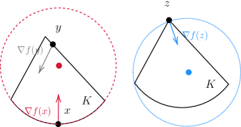
Figure 1: Examples of sphere-enclosed sets.

The Euclidean ball of radius $r$ is $1/r$-strongly convex w.r.t. $\|\cdot\|_{2}$ (Journée et al., 2010, Example 13), and Garber and Hazan (2015, Section 5) provides various examples of strongly convex sets.

In this paper, we introduce a new, different characterization of convex bodies.

Definition 3 (sphere-enclosed sets).

Let $K\subset\mathbb{R}^{d}$ be a convex body, $u\in\operatorname{bd}(K)$, and $f\colon K\to\mathbb{R}$. Then, convex body $K$ is $(\rho,u,f)$-sphere-enclosed (or simply sphere-enclosed facing $u$) if there exists a sphere of radius $\rho$ that has $u$ on it, encloses $K$, and the gradient of $f$ at point $u$ is directed towards the center of the sphere. That is, there exists $c\in\mathbb{R}^{d}$ and $\rho\in(0,\infty)$ such that $u\in\operatorname{bd}(\mathbb{B}(c,\rho))$, $K\subseteq\mathbb{B}(c,\rho)$, and there exists $k>0$ such that $u+k\nabla f(u)=c$.

Figure 1 shows examples of sphere-enclosed sets. The area enclosed by the solid black lines is convex body $K$. In the left figure, we can see that $K$ is sphere-enclosed facing $x$ (the red dotted line is the minimum sphere facing $x$), but $K$ is not sphere-enclosed facing $y$. In the right figure, we can see that $K$ is sphere-enclosed facing $z$ (the blue dotted line is the minimum sphere facing $z$ for $K$). Note that the notion of sphere-enclosedness is a local property defined for each point of the boundary of convex bodies, in contrast to the definition of strong convexity. The next section will see that we can achieve a logarithmic regret if $K$ is sphere-enclosed facing at optimal decision $x_{\star}$ (Theorem 9).

2.3.2 Existing Lower Bound

Here, we discuss a lower bound when exploiting the curvature of feasible sets. For $\lambda\in(0,1)$, let

$$W_{\lambda}=\left\{(x,y)\in\mathbb{R}^{2}\colon x^{2}+\frac{y^{2}}{\lambda^{2}}\leq 1\right\}$$ (2)

be an ellipsoid with principal curvature $\lambda$. From Huang et al. (2017, Proposition 4), ellipsoid $W_{\lambda}$ is $\lambda$-strongly convex w.r.t. $\|\cdot\|_{2}$. The following lower bound provided in Huang et al. (2017, Theorem 9) is for this $W_{\lambda}$, which matches the upper bound in Huang et al. (2017, Theorem 5).

Theorem 4.

Consider online linear optimization. Let $\lambda,L\in(0,1)$ and $K=W_{\lambda}$. Then, for any algorithm, there exists a sequence of loss functions $f_{1},\dots,f_{T}$ satisfying $f_{t}(\cdot)=\langle g_{t},\cdot\rangle$, $g_{1},\dots,g_{T}\in\{(1,-L),(-1,-L)\}$, and the growth condition that $\|g_{1}+\dots+g_{t}\|_{2}\geq tL$ for all $t\in[T]$ such that $\mathsf{R}_{T}\geq\frac{1}{84\sqrt{2}}\frac{1}{\lambda L}\ln T-\delta$ for $\delta=\frac{1}{\lambda L}\left(\frac{2}{1-\mathrm{e}^{\lambda^{2}L^{2}}}+\frac{\pi^{2}}{108}\right)$.

In their proof, they use the following sequence of linear functions $f_{t}(\cdot)=\langle h_{t}^{L},\cdot\rangle$. Let $P$ be a random variable following a Beta distribution, $\mathrm{Beta}(k,k)$, for some $k>0$. For this $P$, let $(X_{t})_{t=1}^{T}$ be i.i.d. random variables following a Bernoulli distribution with parameter $P$. Then for $L\in(0,1)$, let $h_{t}^{L}=(2X_{t}-1,-L)$, which indeed satisfies $\|g_{1}+\dots+g_{t}\|_{2}\geq tL$ for all $t\in[T]$ in Theorem 4. This construction of loss functions will also be used to prove lower bounds in Section 3, and we will provide a matching upper bound in Corollary 11.

2.4 Universal Online Learning

Our algorithm is based on the results of universal online learning. In the literature, the following regret upper bound is the crux for being adaptivity to the curvature of loss functions:

Lemma 5.

Consider online convex optimization. Then, there exists an (efficient) algorithm such that $\sum_{t=1}^{T}\langle\nabla f_{t}(x_{t}),x_{t}-x_{\star}\rangle$ is bounded from above by

$$O\Bigg{(}\min\Bigg{\{}c_{\mathsf{sc}}\sqrt{\sum_{t=1}^{T}\|x_{t}-x_{\star}\|_{2}^{2}\,\ln T}+c_{\mathsf{sc}}^{\prime}\ln T\,,\,c_{\mathsf{ec}}\sqrt{\sum_{t=1}^{T}\left(\langle\nabla f_{t}(x_{t}),x_{t}-x_{\star}\rangle\right)^{2}\,\ln T}+c_{\mathsf{ec}}^{\prime}\ln T\,,\,GD\sqrt{Tc_{\mathsf{g}}}\Bigg{\}}\Bigg{)}\,,$$ (3)

where $c_{\mathsf{sc}},c_{\mathsf{sc}}^{\prime},c_{\mathsf{ec}},c_{\mathsf{ec}}^{\prime},c_{\mathsf{g}}>0$ are algorithm dependent variables provided in the following.

For example, upper bound (3) can be achieved by

• MetaGrad algorithm with $c_{\mathsf{sc}}=G\sqrt{d}$, $c_{\mathsf{sc}}^{\prime}=d$, $c_{\mathsf{ec}}=\sqrt{d}$, $c_{\mathsf{ec}}^{\prime}=d$, and $c_{\mathsf{g}}=\ln\ln T$ (van Erven and Koolen, 2016; van Erven et al., 2021);

• Maler algorithm with $c_{\mathsf{sc}}=G$, $c_{\mathsf{sc}}^{\prime}=GD$, $c_{\mathsf{ec}}=\sqrt{d}$, $c_{\mathsf{ec}}^{\prime}=GD+d$, and $c_{\mathsf{g}}=1$ (Wang et al., 2020, Theorem 1).

We will see that our regret bounds depend on $c_{\mathsf{sc}},c_{\mathsf{sc}}^{\prime},c_{\mathsf{ec}},c_{\mathsf{ec}}^{\prime},c_{\mathsf{g}}>0$, and one can use any algorithm with bound (3).

3 Regret Lower Bounds

In this section, we construct lower bounds that align with the assumptions of our regret bounds. Considering a sequence of loss functions to construct the lower bound in Theorem 4, we can immediately obtain the following lower bound.

Theorem 6.

Consider online linear optimization. Let $\lambda,L\in(0,1)$ and $K=W_{\lambda}$. Then, for any algorithm, there exists a stochastic sequence of loss functions $f_{1},\dots,f_{T}$ satisfying $f_{t}(\cdot)=\langle g_{t},\cdot\rangle$, $g_{1},\dots,g_{T}\in\{(1,-L),(-1,-L)\}$, and $\|\nabla f^{\circ}(x_{t})\|_{2}=L$ such that

$$\mathsf{R}_{T}\geq\frac{1}{84\sqrt{2}}\frac{1}{\lambda\|\nabla f^{\circ}(x_{\star})\|}_{2}\ln T-\delta\,,$$ (4)

where $\delta$ is defined in Theorem 4.

Proof.

Consider the sequence of loss vectors $h_{1}^{L},\dots,h_{T}^{L}$ after Theorem 4 and let $f_{t}(\cdot)=\langle h_{t}^{L},\cdot\rangle$ for all $t\in[T]$. For this sequence of $(f_{t})_{t=1}^{T}$, it holds that $\|\nabla f^{\circ}(x_{t})\|_{2}=\|\mathbb{E}{\left[h_{t}^{L}\right]}\|_{2}=\|\left(0,-L\right)\|_{2}=L\neq 0,$ which completes the proof. ∎

With this lower bound, we can prove the following lower bound for corrupted stochastic environments.

Theorem 7.

Consider online linear optimization. Let $\lambda,L\in(0,1)$ and $K=W_{\lambda}$. Suppose that $T\geq C/(\lambda L)^{2}$ and $C\geq 1/(\lambda L)$. Then, for any algorithm, there exists a corrupted stochastic environment with corruption level at most $C\geq 0$ satisfying $\|\nabla f^{\circ}(x_{t})\|_{2}=L$ such that

$$\mathsf{R}_{T}\geq\frac{1}{168\sqrt{2}}\left(\frac{1}{\lambda\|\nabla f^{\circ}(x_{t})\|_{2}}+\sqrt{\frac{C}{\lambda\|\nabla f^{\circ}(x_{t})\|_{2}}}\right)\sqrt{\ln\left(\frac{C}{\lambda\|\nabla f^{\circ}(x_{t})\|_{2}}\right)}-\delta\,,$$

where $\delta$ is defined in Theorem 4.

The assumption that $T\geq C/(\lambda L)^{2}$ makes some sense since the construction of this lower bound relies on Theorem 6, and if the assumption does not hold then the lower bound becomes vacuous.

Proof.

We will construct a sequence of $f_{1},\dots,f_{T}$ in a corrupted stochastic environment, where $f_{1},\dots,f_{T}$ are generated so that $\widetilde{f}_{t}(\cdot)=\langle\widetilde{g}_{t},\cdot\rangle$ with $\widetilde{g}_{1},\dots,\widetilde{g}_{T}$ following some distribution $\mathcal{D}$ and $f_{t}$ is a corrupted function of $\widetilde{f}_{t}$.

We first note that we have $T\geq C/(\lambda L)\geq 1/(\lambda L)^{2}$. Define $\widehat{L}>0$ such that $\lambda\widehat{L}=\sqrt{\lambda L/C}$. Note that since $C\geq 1/(\lambda L)$, it holds that $\lambda\widehat{L}\leq\lambda L$, implying that $\widehat{L}\in(0,1)$. We also define $\tau\coloneqq\left\lceil\frac{1}{(\lambda\widehat{L})^{2}}\right\rceil=\left\lceil\frac{C}{\lambda L}\right\rceil\leq T$, where the equality holds by $\lambda\widehat{L}=\sqrt{\lambda L/C}$ and the inequality by $T\geq C/(\lambda L)$.

Using these definitions, we consider the following corrupted stochastic environments with corruption level at most $C$:

• For $t\in\{1,\dots,\tau\}$, define $\widetilde{f}_{t}$ by $\widetilde{f}_{t}(\cdot)=\langle\widetilde{g}_{t},\cdot\rangle$ for $\widetilde{g}_{t}=h_{t}^{L}$, where $h_{t}^{L}$ is defined after Theorem 6, and define loss function $f_{t}$ by $f_{t}(\cdot)=\langle g_{t},\cdot\rangle$ with $g_{t}=h_{t}^{\widehat{L}}$.

• For $t\in\{\tau+1,\dots,T\}$, let $\widetilde{f}_{t}(\cdot)=f_{t}(\cdot)=\langle g_{t},\cdot\rangle$ with $g_{t}=h_{t}^{L}$, in which no corruption is introduced.

In fact, the corruption level of this environment is bounded by $C$ since $\sum_{t=1}^{T}\mathbb{E}\big{[}\|f_{t}-\widetilde{f}_{t}\|_{\infty}\big{]}=\sum_{t=1}^{\tau}\big{[}\sup_{x\in K}\lvert\langle g_{t}-\widetilde{g}_{t},x\rangle\rvert\big{]}\leq\tau\lvert L-\widehat{L}\rvert\lambda\leq\left\lceil\frac{C}{\lambda L}\right\rceil\cdot\lvert L-\widehat{L}\rvert\lambda\leq C,$ where in the first inequality we used the fact that the first elements of $g_{t}$ and $\widetilde{g}_{t}$ are the same and that $K=W_{\lambda}$. This implies that the sequence of $(f_{t})_{t=1}^{T}$ is a corrupted stochastic environment with corruption level at most $C$.

Hence, from Theorem 6 with $\widehat{L}\in(0,1)$, $\lambda\widehat{L}=\sqrt{\lambda L/C}$, and the definition of $\tau$, the regret is bounded from below as $\mathsf{R}_{T}\geq\frac{1}{84\sqrt{2}}\frac{1}{\lambda\widehat{L}}\ln\tau-\delta\geq\frac{1}{84\sqrt{2}}\sqrt{\frac{C}{\lambda L}\ln\left(\frac{C}{\lambda L}\right)}-\delta\geq\frac{1}{84\sqrt{2}}\frac{1}{\lambda L}\ln\left(\frac{C}{\lambda L}\right)-\delta,$ which completes the proof. ∎

4 Regret Upper Bounds

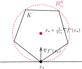
Figure 2: The region enclosed by the black solid line is feasible set $K$ and the red dotted line $B_{\gamma_{\star}}^{K}$ is the smallest sphere enclosing $K$ and facing $x_{\star}$.

In this section, we provide regret upper bounds that nearly match the lower bounds in Section 3, by the universal online learning framework, whose regret is bounded as (3). Note that this section works with convex loss functions.

4.1 Stochastic Environment

We provide logarithmic regret for stochastic environments. Define ball $B_{\gamma}^{K}\subset\mathbb{R}^{d}$ for $\gamma>0$ by

$$B_{\gamma}^{K}=\mathbb{B}\left(x_{\star}+\frac{1}{2\gamma}\nabla f^{\circ}(x_{\star})\,,\,\frac{1}{2\gamma}\left\|\nabla f^{\circ}(x_{\star})\right\|_{2}\right)\,.$$ (5)

By the definition, it holds that $x_{\star}\in\operatorname{bd}(B_{\gamma}^{K})$. See Figure 2.

Remark 8.

The ball $B_{\gamma}^{K}$ is determined in the following manner. We will see in the following proof that inequality $\left\langle\nabla f^{\circ}(x_{\star}),x_{t}-x_{\star}\right\rangle\geq\gamma\|x_{t}-x_{\star}\|_{2}^{2}$ for some $\gamma>0$ plays a key role in proving a logarithmic regret. This inequality is equivalent to $\left\|x_{t}-\left(x_{\star}+\frac{1}{2\gamma}\nabla f^{\circ}(x_{\star})\right)\right\|_{2}\leq\frac{1}{2\gamma}\left\|\nabla f^{\circ}(x_{\star})\right\|_{2}$ and we define $B_{\gamma}^{K}$ as the set of all $x_{t}\in\mathbb{R}^{d}$ satisfying this inequality.

Using this $B_{\gamma}^{K}$, we let $\gamma_{\star}=\sup\{\gamma\geq 0\colon K\subseteq B_{\gamma}^{K}\}$. Then, we can prove the following theorem.

Theorem 9.

Consider online convex optimization in stochastic environments, where the optimal decision is $x_{\star}=\operatorname*{arg\,min}_{x\in K}f^{\circ}(x)$. Suppose that $K$ is $(\rho,x_{\star},f^{\circ})$-sphere-enclosed and that $\nabla f^{\circ}(x_{\star})\neq 0$. Then, any algorithm with bound (3) achieves

$$\mathsf{R}_{T}=O\left(\frac{c_{\mathsf{sc}}^{2}}{\gamma_{\star}}\ln T+c_{\mathsf{sc}}^{\prime}\ln T\right)=O\left(\frac{c_{\mathsf{sc}}^{2}\,\rho}{\|\nabla f^{\circ}(x_{\star})\|}_{2}\ln T+c_{\mathsf{sc}}^{\prime}\ln T\right)\,.$$

We will see in Corollary 11 that this upper bound matches the lower bound in Theorem 6 in the environment used to construct the lower bound.

Proof.

The regret is bounded from below by

$$\mathsf{R}_{T}=\mathbb{E}{\left[\sum_{t=1}^{T}\left(f^{\circ}(x_{t})-f^{\circ}(x_{\star})\right)\right]}\geq\mathbb{E}{\left[\sum_{t=1}^{T}\langle\nabla f^{\circ}(x_{\star}),x_{t}-x_{\star}\rangle\right]}\geq\mathbb{E}{\left[\sum_{t=1}^{T}\gamma_{\star}\|x_{t}-x_{\star}\|_{2}^{2}\right]}\,,$$ (6)

where the first inequality follows by the convexity of $f^{\circ}$, and the last inequality follows by $x_{t}\in K\subseteq B_{\gamma_{\star}}^{K}$ and the definition of $\gamma_{\star}$. By combining this inequality with inequality (3), the regret is bounded as $\mathsf{R}_{T}\leq\mathbb{E}{\left[\sum_{t=1}^{T}\langle\nabla f_{t}(x_{t}),x_{t}-x_{\star}\rangle\right]}=O\left(c_{\mathsf{sc}}\sqrt{\frac{\mathsf{R}_{T}}{\gamma_{\star}}\ln T}+c_{\mathsf{sc}}^{\prime}\ln T\right).$ Solving this inequation w.r.t. $\mathsf{R}_{T}$, we get $\mathsf{R}_{T}=O\left(\frac{c_{\mathsf{sc}}^{2}}{\gamma_{\star}}\ln T+c_{\mathsf{sc}}^{\prime}\ln T\right).$ Observing that $\frac{1}{2\gamma_{\star}}\|\nabla f^{\circ}(x_{\star})\|_{2}=\rho$, which holds from the assumption that $K$ is $(\rho,x_{\star},f^{\circ})$-sphere-enclosed, we complete the proof. ∎

The advantages of the regret bound in Theorem 9 compared to the existing upper bounds are the following: (i) The logarithmic regret can be achieved as long as the boundary of $K$ is curved around the optimal decision $x_{\star}$ or $x_{\star}$ in on corners (see Figure 1), while the existing analysis requires strong convexity over the entire feasible set $K$. (ii) While the existing analysis only considers linear loss functions, our approach can handle convex loss functions and thus the curvature of loss functions (e.g., strong convexity or exp-concavity) can be simultaneously exploited (see Section 4.3). (iii) Even if the assumptions on loss vectors $g_{1},\dots,g_{T}$ are not satisfied, the $O(\sqrt{T})$ regret upper bound can be achieved, while the existing approach, FTL, can suffer $\Omega(T)$ regret.

A limitation of the proposed approach is that it assumes stochastic environments. However, our approach at least guarantees an $O(\sqrt{T})$ bound in the (fully) adversarial environments, where the growth assumption needed for FTL to achieve the fast rates is not satisfied, and as we will see in the following section, we can achieve the fast rates also in corrupted stochastic environments.

For the assumption on loss vectors, the existing studies consider the following assumptions on loss vectors $g_{t}$: There exists $L>0$ such that $\|g_{1}+\dots+g_{T}\|_{2}\geq tL$ for all $t\in[T]$, or $g_{t}\leq 0$ for all $t\in[T]$. These assumptions cannot be directly comparable with our assumption that $\nabla f^{\circ}(x_{\star})\neq 0$. Note that the assumption that $\inf_{x\in K}\|\nabla f^{\circ}(x)\|>0$ is standard in the literature of offline optimization, when deriving the fast convergence rate, see Levitin and Polyak (1966); Demyanov and Rubinov (1970); Dunn (1979) and discussion in Garber and Hazan (2015) for details.

Tightness of regret upper bound in Theorem 9

In the remainder of this subsection, we investigate the tightness of the regret upper bound in Theorem 9. To see the tightness of our regret bound, we consider the case when $K$ is an ellipsoid. The following proposition implies that the regret upper bound in Theorem 9 matches the lower bound in Theorem 6.

Proposition 10.

For $\lambda\in(0,1)$, let $W_{\lambda}$ be the ellipsoid defined in (2). Then, its minimum enclosing sphere constrained so that having $(0,-\lambda)$ on it is $\Big{\{}(x,y)\in\mathbb{R}^{2}\colon x^{2}+\Big{(}y-\frac{1-\lambda^{2}}{\lambda}\Big{)}^{2}=\frac{1}{\lambda^{2}}\Big{\}}\,.$

The proof of Proposition 10 is deferred to Appendix A. This result immediately implies the following matching regret upper bound.

Corollary 11.

Let $K$ be $W_{\lambda}$ and $x^{*}=(0,-\lambda)$. Under the same assumption as in Theorem 9, in the environment considered in the construction of the lower bound in Theorem 4, the algorithm in Wang et al. (2020) achieves $\mathsf{R}_{T}=O\left(\frac{1}{\lambda L}\ln T+GD\ln T\right).$

We can see that this upper bound matches the lower bound in Theorem 6 up to the additive $GD\ln T$ factor.

Proof.

From Proposition 10 and the fact that Euclidean ball with radius $r$ is $1/r$ strongly convex w.r.t. $\|\cdot\|_{2}$, we have $\rho=1/\lambda$. This proposition combined with Theorem 9 immediately gives the desired bound. ∎

The upper bound in Theorem 9 is applicable when $K$ is a polytope. We will see that our approach work also in the corrupted stochastic environment in Section 4.2, and to our knowledge, this is the first upper bound that achieves fast rates when the feasible set is a polytope in non-stochastic environments. A further discussion when $K$ is a polytope can be found in Appendix B.

4.2 Corrupted Stochastic Environments

Another advantage of our approach is that it can achieve nearly optimal regret upper bounds even in corrupted stochastic environments. for this $\widetilde{B}_{\gamma}^{K}$, we let $\widetilde{\gamma}_{\star}=\sup\{\gamma\geq 0\colon K\subseteq\widetilde{B}_{\gamma}^{K}\}.$ For $\gamma>0$, we define ball $\widetilde{B}_{\gamma}^{K}\subset\mathbb{R}^{d}$ by $\widetilde{B}_{\gamma}^{K}=\mathbb{B}\big{(}\widetilde{x}_{\star}+\frac{1}{2\gamma}\nabla\widetilde{f}^{\circ}(\widetilde{x}_{\star})\,,\,\frac{1}{2\gamma}\big{\|}\nabla\widetilde{f}^{\circ}(\widetilde{x}_{\star})\big{\|}_{2}\big{)}\,,$ which is defined in the same manner as $B_{\gamma}^{K}$. Then, we can prove the following regret upper bound.

Theorem 12.

Consider online convex optimization in corrupted stochastic environments with corruption level at most $C$, where $\widetilde{x}_{\star}=\operatorname*{arg\,min}_{x\in K}\widetilde{f}^{\circ}(x)$. Suppose $K$ is $(\rho,\widetilde{x}_{\star},\widetilde{f}^{\circ})$-sphere enclosed and $\nabla\widetilde{f}^{\circ}(\widetilde{x}_{\star})\neq 0$. Then, any algorithm with bound (3) achieves

$$\mathsf{R}_{T}=O\left(\frac{c_{\mathsf{sc}}^{2}}{\widetilde{\gamma}_{\star}}\ln T+\sqrt{\frac{Cc_{\mathsf{sc}}^{2}}{\widetilde{\gamma}_{\star}}\ln T}+c_{\mathsf{sc}}^{\prime}\ln T\right)=O\left(\frac{c_{\mathsf{sc}}^{2}\,\rho}{\|\nabla\widetilde{f}^{\circ}(\widetilde{x}_{\star})\|}_{2}\ln T+\sqrt{\frac{Cc_{\mathsf{sc}}^{2}\,\rho}{\|\nabla\widetilde{f}^{\circ}(\widetilde{x}_{\star})\|}_{2}\ln T}+c_{\mathsf{sc}}^{\prime}\ln T\right)\,.$$

The proof of Theorem 12 can be found in Appendix C. We can observe that this upper bound matches the lower bound in Theorem 7 up to logarithmic factors, considering the environment to prove the lower bound. It is worth mentioning that all upper bounds provided in this paper can be extended following the same line as the proof of Theorem 12.

4.3 Exploiting the Curvature of Loss Functions and Feasible Sets Simultaneously

One of the advantages of directly solving OCO over reducing to OLO is that we can obtain upper bounds that can simultaneously exploit the curvature of feasible sets and loss functions:

Theorem 13.

Suppose that the same assumption as in Theorem 9 holds. If $f_{1},\dots,f_{T}$ are $\alpha$-strongly convex w.r.t. a norm $\|\cdot\|$, then $\mathsf{R}_{T}=O\left(\frac{c_{\mathsf{sc}}^{2}}{\gamma_{\star}+\alpha/\xi}\ln T+c_{\mathsf{sc}}^{\prime}\ln T\right).$ If $f_{1},\dots,f_{T}$ are $\beta$-exp-concave, then $\mathsf{R}_{T}=O\left(\min\left\{\frac{c_{\mathsf{sc}}^{2}}{\gamma_{\star}}\,,\frac{c_{\mathsf{ec}}^{2}}{\beta^{\prime}+\gamma_{\star}/G^{2}}\right\}\ln T+\max\left\{c_{\mathsf{sc}}^{\prime},c_{\mathsf{ec}}^{\prime}\right\}\ln T\right)$ for $\beta^{\prime}\leq\frac{1}{2}\min\left\{\frac{1}{4GD},\beta\right\}$.

The proof can be found in Appendix D. Theorem 13 implies that one can simultaneously exploit the curvature of feasible sets and loss functions. Note that the similar analysis is possible for corrupted stochastic environments.

4.4 Extending Analysis to Uniformly Convex Sets

Here, we prove that a regret upper bound smaller than $O(\sqrt{T})$ can be achieved when $K$ is uniformly convex. This can be proven by essentially a similar argument using the idea of exploiting the lower bound, as done in the proof for sphere-enclosed sets.

Definition 14.

A convex body $K$ is $(\kappa,q)$-uniformly convex w.r.t. a norm $\|\cdot\|$ (or $q$-uniformly convex) if for any $x,y\in K$ and any $\theta\in[0,1]$, it holds that $\theta x+(1-\theta)y+\theta(1-\theta)\frac{\kappa}{2}\|x-y\|^{q}\cdot\mathbb{B}_{\|\cdot\|}\subseteq K\,.$

For $p\geq 2$, $\ell_{p}$-balls are $(1/p,p)$-uniformly convex w.r.t. $\|\cdot\|_{p}$ for $p\geq 2$ (Hanner, 1956, Theorem 2), and $p$-Schatten balls are $(1/p,p)$-uniformly convex w.r.t. the Schatten norm $\|\cdot\|_{S(p)}$ (See Kerdreux et al. (2021a) for the connection between the uniform convexity of a normed space and the uniform convexity of sets.) Note that $(\kappa,2)$-uniformly convex set is $\kappa$-strongly convex. For the uniformly convex feasible sets, we can prove the following theorem.

Theorem 15.

Consider online convex optimization in stochastic environments, where the optimal decision is $x_{\star}=\operatorname*{arg\,min}_{x\in K}f^{\circ}(x)$. Suppose that $K$ is $(\kappa,q)$-uniformly convex w.r.t. a norm $\|\cdot\|$ for some $q\geq 2$ and that $\nabla f^{\circ}(x_{\star})\neq 0$. Then, any algorithm with bound (3) achieves

$$\mathsf{R}_{T}=\left(\frac{\left(\xi c_{\mathsf{sc}}\right)^{\frac{q}{q-1}}}{\left(q\kappa\|\nabla f^{\circ}(x_{\star})\|_{\star}\right)^{\frac{1}{q-1}}}T^{\frac{q-2}{2(q-1)}}\left(\ln T\right)^{\frac{q}{2(q-1)}}+c_{\mathsf{sc}}^{\prime}\ln T\right)\,.$$ (7)

In particular, when $K$ is $\lambda$-strongly convex w.r.t. a norm $\|\cdot\|$, $\mathsf{R}_{T}=O\left(\frac{\xi c_{\mathsf{sc}}}{\lambda\|\nabla f^{\circ}(x_{\star})\|_{\star}}\ln T+c_{\mathsf{sc}}^{\prime}\ln T\right)\,.$

The dependence on $T$ in this bound is $O\left(T^{\frac{q-2}{2(q-1)}}\left(\ln T\right)^{\frac{q}{2(q-1)}}\right)$, which becomes $O(\ln T)$ when $q=2$ and $\widetilde{O}(\sqrt{T})$ when $q\to\infty$, and thus interpolates between the bound over the strongly convex sets and non-curved feasible sets. This is strictly better than the $O\left(T^{\frac{q-2}{q-1}}\right)$ bound in Kerdreux et al. (2021a); their regret upper bound is better than $O(\sqrt{T})$ only when $q\in(2,3)$. For example, when $K$ is $\ell_{p}$-ball, by $\|x\|_{2}\leq d^{\frac{1}{2}-\frac{1}{p}}\|x\|_{p}$ for any $x\in\mathbb{R}^{d}$ and $p>2$, the regret is bounded as $\mathsf{R}_{T}=O\bigg{(}\frac{\left(\xi c_{\mathsf{sc}}\right)^{\frac{p}{p-1}}d^{\frac{p-2}{2(p-1)}}}{\left(\|\nabla f^{\circ}(x_{\star})\|_{\star}\right)^{\frac{1}{p-1}}}T^{\frac{p-2}{2(p-1)}}\left(\ln T\right)^{\frac{p}{2(p-1)}}+c_{\mathsf{sc}}^{\prime}\ln T\bigg{)}.$ Note that the similar analysis is possible for corrupted stochastic environments.

Before proving the theorem, we present the following lemma, which offers a characterization of uniformly convex sets. This directly follows from the definition in Definition 14:

Lemma 16.

Suppose that a convex body $K$ is $(\kappa,q)$-uniformly convex w.r.t. a norm $\|\cdot\|$ for $\kappa>0$ and $q\geq 2$. Let $y\in K$, $g\in\mathbb{R}^{d}$, and $y_{\star}\in\operatorname*{arg\,min}_{y^{\prime}\in K}\langle g,y^{\prime}\rangle$. Then it holds that

$$\langle-g,y_{\star}-y\rangle\geq\frac{\kappa}{2}\|y-y_{\star}\|^{q}\cdot\|g\|_{\star}\,.$$ (8)

The proof of this lemma can be found in Kerdreux et al. (2021b, Lemma 2.1), and we will include the proof in Appendix E for completeness.

Proof.

From $x_{\star}=\operatorname*{arg\,min}_{x\in K}f^{\circ}(x)$ and the first-order optimality condition, $\langle\nabla f^{\circ}(x_{\star}),x-x_{\star}\rangle\geq 0$, which implies that $x_{\star}=\operatorname*{arg\,min}_{x\in K}\langle\nabla f^{\circ}(x_{\star}),x\rangle$. Hence, by combining this with Lemma 16 and that $K$ is $(\kappa,q)$-uniformly convex w.r.t. a norm $\|\cdot\|$, we have $\langle\nabla f^{\circ}(x_{\star}),x-x_{\star}\rangle\geq\frac{\kappa}{2}\|x-x_{\star}\|^{q}\cdot\|\nabla f^{\circ}(x_{\star})\|_{\star}$ for all $x\in K$. Using this inequality,

$$\mathsf{R}_{T} =\mathbb{E}{\left[\sum_{t=1}^{T}\left(f^{\circ}(x_{t})-f^{\circ}(x_{\star})\right)\right]}\geq\mathbb{E}{\left[\sum_{t=1}^{T}\langle\nabla f^{\circ}(x_{\star}),x_{t}-x_{\star}\rangle\right]}$$

$$\geq\frac{\kappa}{2}\|\nabla f^{\circ}(x_{\star})\|_{\star}\cdot\mathbb{E}{\left[\sum_{t=1}^{T}\|x-x_{\star}\|^{q}\right]}\geq\frac{\kappa}{2\xi^{q}}\|\nabla f^{\circ}(x_{\star})\|_{\star}\cdot\mathbb{E}{\left[\sum_{t=1}^{T}\|x-x_{\star}\|_{2}^{q}\right]}$$

$$\geq\frac{\kappa}{2\xi^{q}}\|\nabla f^{\circ}(x_{\star})\|_{\star}\,T^{1-\frac{q}{2}}\left(\mathbb{E}{\left[\sum_{t=1}^{T}\|x-x_{\star}\|_{2}^{2}\right]}\right)^{q/2}\,,$$ (9)

where the first inequality follows by the convexity of $f^{\circ}$, the second inequality by $\|x\|_{2}\leq\xi\|x\|$ for any $x\in\mathbb{R}^{d}$, and the last inequality by Jensen’s inequality and the fact that $x\mapsto x^{q/2}$ is convex for $q\geq 2$. Combining (3) and (9), we can bound the regret as

$$\mathsf{R}_{T}=2\mathsf{R}_{T}-\mathsf{R}_{T}$$

$$=O\left(c_{\mathsf{sc}}\sqrt{\mathbb{E}{\left[\sum_{t=1}^{T}\|x_{t}-x_{\star}\|_{2}^{2}\right]}\ln T}-\frac{\kappa}{\xi^{q}}\|\nabla f^{\circ}(x_{\star})\|_{\star}\,T^{1-\frac{q}{2}}\left(\mathbb{E}{\left[\sum_{t=1}^{T}\|x-x_{\star}\|_{2}^{2}\right]}\right)^{q/2}+c_{\mathsf{sc}}^{\prime}\ln T\right)$$

$$=O\left(\frac{\left(\xi c_{\mathsf{sc}}\right)^{\frac{q}{q-1}}}{\left(q\kappa\|\nabla f^{\circ}(x_{\star})\|_{\star}\right)^{\frac{1}{q-1}}}T^{\frac{q-2}{2(q-1)}}\left(\ln T\right)^{\frac{q}{2(q-1)}}+c_{\mathsf{sc}}^{\prime}\ln T\right)\,,$$ (10)

where in the last line we used the inequality $a\sqrt{x}-bx^{q/2}\leq\frac{a^{\frac{q}{q-1}}}{(qb)^{\frac{1}{q-1}}}$ that holds for $a,b,x>0$ and $q\geq 2$. This completes the proof. ∎

5 Conclusion

In this paper, we considered online convex optimization and designed a new approach to achieve fast rates by exploiting the curvature of feasible sets. In particular, by the algorithm adaptive to the curvature of loss functions, we proved an $O(\rho\ln T)$ regret bound for $(\rho,x_{\star},f^{\circ})$-sphere enclosed feasible sets. There are several advantages of our approach: it can exploit the curvature of loss functions, can achieve the $O(\ln T)$ regret bound only with local curvature properties, and can work robustly even in environments where loss vectors do not satisfy the ideal conditions. Notably, following the similar analysis ideas, we proved the fast rates for uniformly convex feasible sets, which include strongly convex sets and $\ell_{p}$-balls for $p>2$ as special cases. This regret bound interpolates the $O(\ln T)$ regret over strongly convex sets and the $O(\sqrt{T})$ regret over non-curved sets.

Appendix A Proof of Proposition 10

Proof.

Since $K$ is $W_{\lambda}$ and $x_{\star}=(0,-\lambda)$, the optimization problem we need to solve is fomulated as follows:

$$\operatorname*{minimize}_{r>0,\,c>0}\quad r^{2}\quad\mathrm{s.t.}\quad\sup_{(x,y)\in K}\left\|\begin{pmatrix}x\\ y\end{pmatrix}-\begin{pmatrix}0\\ c\end{pmatrix}\right\|^{2}\leq r^{2}\,,\;\text{$\mathbb{B}((0,c),r)$ is tangent to $x_{\star}$}\,.$$ (11)

From geometric observations, we have $c-r=-\lambda$. Hence, the optimization problem (11) can be rewritten as

$$\operatorname*{minimize}_{c\in\mathbb{R}}\quad(c+\lambda)^{2}\quad\mathrm{s.t.}\quad\sup_{(x,y)\in K}\{x^{2}+y^{2}-2cy\}\leq 2c\lambda+\lambda^{2}\,.$$ (12)

In the following, to make the constraint in the optimization problem (12) simpler, we consider the following optimization problem:

$$\operatorname*{maximize}_{(x,y)\in\mathbb{R}^{2}}\quad{x^{2}+y^{2}-2cy}\quad\mathrm{s.t.}\quad x^{2}+\frac{y^{2}}{\lambda^{2}}\leq 1\,.$$ (13)

By the standard method of Lagrange multiplier, one can compute that the optimal value of this optimization problem is $\max\left\{-2\lambda c+\lambda^{2},2\lambda c+\lambda^{2},\frac{1}{\frac{1}{\lambda^{2}}-1}c^{2}+1\right\}\,.$ Since the inequality

$$\max\left\{-2\lambda c+\lambda^{2},2\lambda c+\lambda^{2},\frac{1}{\frac{1}{\lambda^{2}}-1}c^{2}+1\right\}\leq 2\lambda c+\lambda^{2}$$ (14)

only holds when $c=\frac{1-\lambda^{2}}{\lambda}$, the feasible set of the optimization problem (12) is singleton set $\left\{\frac{1-\lambda^{2}}{\lambda}\right\}$. Combining this fact with $c-r=-\lambda$, we get the desired result. ∎

Appendix B Discussion when Feasible Set is Polytope

Here we discuss pros/cons of our regret bound against an existing bound when feasible set $K$ is a polytope. The results mentioned in Section 4 mainly focus on the case where the feasible set is curved. However, as one can see from the definition of the sphere-enclosedness, even if the feasible set is polytope or does not have the curvature, a regret upper bound better than $O(\sqrt{T})$ can be achieved.

In the existing study, the following upper bound in known in stochastic OCO over polytope (Huang et al., 2017, Corollary 11).

Theorem 17.

Consider online online linear optimization in stochastic environments with $g^{\circ}=\mathbb{E}{\left[g_{t}\right]}$. Assume that $K$ is polytope and $\|g_{t}\|_{\infty}\leq M$. Further assume that there exsits $r>0$ such that $\Phi(\cdot)=\max_{x\in K}\langle x,\cdot\rangle$ is differentiable for any $\nu$ such that $\|\nu-g^{\circ}\|\leq r$. Then, the regret of FTL is bounded by $\mathsf{R}_{T}=O\left(\frac{M^{3}D}{r^{2}}\ln\left(\frac{M^{2}d}{r^{2}}\right)\right).$

The comparison of this bound with our regret upper bound is not straightforward. If $\nabla f^{\circ}(x_{\star})$ is not toward the “unfavorable” direction in $K$, then it is trivial that polytope $K$ is $(\rho,x_{\star},f^{\circ})$-sphere-enclosed for some $\rho$, and thus the regret bound in Theorem 9 can be achieved. When $T$ is large enough, the bound in Theorem 17 is better since it does not depend on $T$. However, their regret upper bound depends on $1/r^{2}$ and $M^{3}$, and the relation between them and $1/\|\nabla f^{\circ}(x_{t})\|_{2}$ is unclear, and our bound can be smaller than their bound. Note that the “unfavorable” direction coincide between these upper bounds when OLO is considered.

While the direct comparison is not straightforward, we would like to emphasize that our regret upper bound, in contrast to their bound, is obtained as a corollary of the general analysis, and our bound inherits all the advantages discussed in Section 4. In particular, while their bound is valid only in stochastic environments, our regret guarantee is valid in stochastic, adversarial, and corrupted stochastic environments.

Appendix C Proof of Theorem 12

Proof.

Recalling that $\widetilde{x}_{\star}=\operatorname*{arg\,min}_{x\in K}\widetilde{f}^{\circ}(x)$, we can bound the regret from below as

$$\mathsf{R}_{T} =\max_{x\in K}\mathbb{E}{\left[\sum_{t=1}^{T}\left(f_{t}(x_{t})-f_{t}(x)\right)\right]}$$

$$=\max_{x\in K}\Bigg{\{}\mathbb{E}{\left[\sum_{t=1}^{T}\left(\widetilde{f}_{t}(x_{t})-\widetilde{f}_{t}(x)\right)\right]}+\mathbb{E}{\left[\sum_{t=1}^{T}\left(\left(f_{t}(x_{t})-\widetilde{f}_{t}(x_{t})\right)-\left(f_{t}(x)-\widetilde{f}_{t}(x)\right)\right)\right]}\Bigg{\}}$$

$$\geq\max_{x\in K}\mathbb{E}{\left[\sum_{t=1}^{T}\left(\widetilde{f}_{t}(x_{t})-\widetilde{f}_{t}(x)\right)\right]}-2C\,.$$ (15)

The first term in the last inequality is further bounded from below as

$$\max_{x\in K}\mathbb{E}{\left[\sum_{t=1}^{T}\left(\widetilde{f}_{t}(x_{t})-\widetilde{f}_{t}(x)\right)\right]}\geq\max_{x\in K}\mathbb{E}{\left[\sum_{t=1}^{T}\left(\widetilde{f}^{\circ}(x_{t})-\widetilde{f}^{\circ}(\widetilde{x}_{\star})\right)\right]}$$

$$\geq\mathbb{E}{\left[\sum_{t=1}^{T}\langle\nabla\widetilde{f}^{\circ}(\widetilde{x}_{\star}),x_{t}-x_{\star}\rangle\right]}\geq\mathbb{E}{\left[\sum_{t=1}^{T}\widetilde{\gamma}_{\star}\|x_{t}-x_{\star}\|_{2}^{2}\right]}\,,$$ (16)

where the first inequality follows by the definition of $\widetilde{x}_{\star}$ and the last inequality follows by $x_{t}\in K\subseteq\widetilde{B}_{\gamma_{\star}}^{K}$. Combining the above inequalities with (3), we have $\mathsf{R}_{T}=O\left(c_{\mathsf{sc}}\sqrt{\frac{\mathsf{R}_{T}+C}{\widetilde{\gamma}_{\star}}\ln T}+c_{\mathsf{sc}}^{\prime}\ln T\right)\,.$ Solving this inequation and following the similar analysis as the proof of Theorem 9 complete the proof. ∎

Appendix D Proof of Theorem 13

Proof.

Following the same argument as in the proof of (6), we have

$$\mathsf{R}_{T}=2\mathsf{R}_{T}-\mathsf{R}_{T}\leq 2\mathsf{R}_{T}-\mathbb{E}{\left[\sum_{t=1}^{T}\gamma_{\star}\|x_{t}-x_{\star}\|_{2}^{2}\right]}\,.$$ (17)

From the strong convexity of $f_{t}$, we also have

$$\mathsf{R}_{T}\leq\mathbb{E}{\left[\sum_{t=1}^{T}\left(\langle\nabla f_{t}(x_{t}),x_{t}-x_{\star}\rangle-\frac{\alpha}{2}\|x_{t}-x_{\star}\|^{2}\right)\right]}\leq\mathbb{E}{\left[\sum_{t=1}^{T}\left(\langle\nabla f_{t}(x_{t}),x_{t}-x_{\star}\rangle-\frac{\alpha}{2\xi}\|x_{t}-x_{\star}\|_{2}^{2}\right)\right]}\,.$$ (18)

Plugging (18) in (17) and from Lemma 5 and Jensen’s inequality,

$$\mathsf{R}_{T} =O\Bigg{(}c_{\mathsf{sc}}\sqrt{\sum_{t=1}^{T}\mathbb{E}{\left[\|x_{t}-x_{\star}\|_{2}^{2}\right]}\ln T}+c_{\mathsf{sc}}^{\prime}\ln T-\left(\frac{\alpha}{\xi}+\gamma_{\star}\right)\mathbb{E}{\left[\sum_{t=1}^{T}\|x_{t}-x_{\star}\|_{2}^{2}\right]}\Bigg{)}$$

$$=O\left(\frac{c_{\mathsf{sc}}^{2}}{\alpha/\xi+\gamma_{\star}}\ln T+c_{\mathsf{sc}}^{\prime}\ln T\right)\,,$$ (19)

which completes the proof for the strongly convex loss functions.

Next, we consider the case where $f_{t}$’s are exp-concave. By Hazan et al. (2007, Lemma 3), the $G$-Lipschitzness and $\beta$-exp-concavity of $f_{t}$ implies

$$f_{t}(x_{\star})\geq f_{t}(x_{t})+\langle\nabla f_{t}(x_{t}),x_{\star}-x_{t}\rangle+\frac{\beta^{\prime}}{2}\left(\langle\nabla f_{t}(x_{t}),x_{t}-x_{\star}\rangle\right)^{2}$$ (20)

for $\beta^{\prime}\leq\frac{1}{2}\min\left\{\frac{1}{4GD},\beta\right\}$. Using this and Lemma 5 to follow a similar argument as the strongly-convex case, we can bound the regret as

$$\mathsf{R}_{T} =O\Bigg{(}\sqrt{\min\left\{c_{\mathsf{sc}}^{2}\mathbb{E}{\left[\sum_{t=1}^{T}\|x_{t}-x_{\star}\|_{2}^{2}\right]}\,,\,c_{\mathsf{ec}}^{2}\mathbb{E}{\left[\sum_{t=1}^{T}\left(\langle\nabla f_{t}(x_{t}),x_{t}-x_{\star}\rangle\right)^{2}\right]}\right\}\ln T}$$

$$\qquad-\gamma_{\star}\mathbb{E}{\left[\sum_{t=1}^{T}\|x_{t}-x_{\star}\|_{2}^{2}\right]}-\beta^{\prime}\mathbb{E}{\left[\sum_{t=1}^{T}\left(\langle\nabla f_{t}(x_{t}),x_{t}-x_{\star}\rangle\right)^{2}\right]}+\max\left\{c_{\mathsf{sc}}^{\prime},c_{\mathsf{ec}}^{\prime}\right\}\ln T\Bigg{)}$$

$$=O\left(\min\left\{\frac{c_{\mathsf{sc}}^{2}}{\gamma_{\star}}\,,\frac{c_{\mathsf{ec}}^{2}}{\beta^{\prime}+\gamma_{\star}/G^{2}}\right\}+\max\left\{c_{\mathsf{sc}}^{\prime},c_{\mathsf{ec}}^{\prime}\right\}\ln T\right)\,,$$ (21)

where in the last inequality we used $\|x_{t}-x_{\star}\|_{2}^{2}\geq\frac{1}{G^{2}}\left(\nabla f_{t}(x_{t})^{\top}(x_{t}-x_{\star})\right)^{2}$ that holds by the Cauchy–Schwarz inequality. ∎

Appendix E Proof of Lemma 16

Proof.

Since $K$ is $(\kappa,q)$-uniformly convex w.r.t. norm $\|\cdot\|$,

$$\frac{y+y_{\star}}{2}+\frac{\kappa}{4}\|y-y_{\star}\|^{q}\cdot\mathbb{B}_{\|\cdot\|}\subseteq K.$$ (22)

Hence, for any $z\in\mathbb{B}_{\|\cdot\|}$, the definition of $y_{\star}$ implies that

$$\langle g,y_{\star}\rangle\leq\left\langle g,\frac{y+y_{\star}}{2}+\frac{\kappa}{4}\|y-y_{\star}\|^{q}z\right\rangle=\left\langle g,\frac{y+y_{\star}}{2}\right\rangle+\left\langle g,\frac{\kappa}{4}\|y-y_{\star}\|^{q}z\right\rangle\,,$$ (23)

Rearranging the last inequality implies $\langle-g,y_{\star}-y\rangle\geq\frac{\kappa}{2}\|y-y_{\star}\|^{q}\langle-g,z\rangle.$ Choosing $z=-g/\|g\|\in\mathbb{B}_{\|\cdot\|}$ completes the proof. ∎

References

• Dekel et al. (2017) Ofer Dekel, Arthur Flajolet, Nika Haghtalab, and Patrick Jaillet. Online learning with a hint. In Advances in Neural Information Processing Systems, volume 30, pages 5299–5308, 2017.
• Demyanov and Rubinov (1970) Vladimir F. Demyanov and Aleksandr M. Rubinov. Approximate methods in optimization problems. Elsevier Publishing Company, 1970.
• Dunn (1979) Joseph C. Dunn. Rates of convergence for conditional gradient algorithms near singular and nonsingular extremals. SIAM Journal on Control and Optimization, 17(2):187–211, 1979.
• Garber and Hazan (2015) Dan Garber and Elad Hazan. Faster rates for the Frank-Wolfe method over strongly-convex sets. In Proceedings of the 32nd International Conference on Machine Learning, volume 37, pages 541–549, 2015.
• Hanner (1956) Olof Hanner. On the uniform convexity of Lp and lp. Arkiv för Matematik, 3(3):239–244, 1956.
• Hazan et al. (2007) Elad Hazan, Amit Agarwal, and Satyen Kale. Logarithmic regret algorithms for online convex optimization. Machine Learning, 69:169–192, 2007.
• Huang et al. (2017) Ruitong Huang, Tor Lattimore, András György, and Csaba Szepesvári. Following the leader and fast rates in online linear prediction: Curved constraint sets and other regularities. Journal of Machine Learning Research, 18(145):1–31, 2017.
• Ito (2021) Shinji Ito. On optimal robustness to adversarial corruption in online decision problems. In Advances in Neural Information Processing Systems, volume 34, pages 7409–7420, 2021.
• Journée et al. (2010) Michel Journée, Yurii Nesterov, Peter Richtárik, and Rodolphe Sepulchre. Generalized power method for sparse principal component analysis. Journal of Machine Learning Research, 11(15):517–553, 2010.
• Kerdreux et al. (2021a) Thomas Kerdreux, Alexandre d’Aspremont, and Sebastian Pokutta. Projection-free optimization on uniformly convex sets. In Proceedings of The 24th International Conference on Artificial Intelligence and Statistics, volume 130, pages 19–27, 2021a.
• Kerdreux et al. (2021b) Thomas Kerdreux, Christophe Roux, Alexandre d’Aspremont, and Sebastian Pokutta. Linear bandits on uniformly convex sets. Journal of Machine Learning Research, 22(284):1–23, 2021b.
• Levitin and Polyak (1966) Evgeny S. Levitin and Boris T. Polyak. Constrained minimization methods. USSR Computational Mathematics and Mathematical Physics, 6(5):1–50, 1966.
• Lykouris et al. (2018) Thodoris Lykouris, Vahab Mirrokni, and Renato Paes Leme. Stochastic bandits robust to adversarial corruptions. In Proceedings of the 50th Annual ACM SIGACT Symposium on Theory of Computing, pages 114–122, 2018.
• Mhammedi (2022) Zakaria Mhammedi. Exploiting the curvature of feasible sets for faster projection-free online learning. arXiv preprint arXiv:2205.11470, 2022.
• Molinaro (2022) Marco Molinaro. Strong convexity of feasible sets in off-line and online optimization. Mathematics of Operations Research, 48(2):865–884, 2022.
• Sachs et al. (2022) Sarah Sachs, Hedi Hadiji, Tim van Erven, and Cristóbal Guzmán. Between stochastic and adversarial online convex optimization: Improved regret bounds via smoothness. In Advances in Neural Information Processing Systems, volume 35, pages 691–702, 2022.
• Sachs et al. (2023) Sarah Sachs, Hedi Hadiji, Tim van Erven, and Cristobal Guzman. Accelerated rates between stochastic and adversarial online convex optimization. arXiv preprint arXiv:2303.03272, 2023.
• van Erven and Koolen (2016) Tim van Erven and Wouter M Koolen. MetaGrad: Multiple learning rates in online learning. In Advances in Neural Information Processing Systems, volume 29, pages 3666–3674, 2016.
• van Erven et al. (2021) Tim van Erven, Wouter M. Koolen, and Dirk van der Hoeven. MetaGrad: Adaptation using multiple learning rates in online learning. Journal of Machine Learning Research, 22(161):1–61, 2021.
• Wang et al. (2020) Guanghui Wang, Shiyin Lu, and Lijun Zhang. Adaptivity and optimality: A universal algorithm for online convex optimization. In Proceedings of The 35th Uncertainty in Artificial Intelligence Conference, volume 115, pages 659–668, 2020.
• Yan et al. (2023) Yu-Hu Yan, Peng Zhao, and Zhi-Hua Zhou. Universal online learning with gradient variations: A multi-layer online ensemble approach. In Advances in Neural Information Processing Systems, volume 36, 2023.
• Zhang et al. (2022) Lijun Zhang, Guanghui Wang, Jinfeng Yi, and Tianbao Yang. A simple yet universal strategy for online convex optimization. In Proceedings of the 39th International Conference on Machine Learning, volume 162, pages 26605–26623, 2022.
• Zinkevich (2003) Martin Zinkevich. Online convex programming and generalized infinitesimal gradient ascent. In Proceedings of the 20th International Conference on Machine Learning, pages 928–936, 2003.