Bounding Reconstruction Attack Success of Adversaries Without Data Priors
Abstract
Reconstruction attacks on machine learning (ML) models pose a strong risk of leakage of sensitive data. In specific contexts, an adversary can (almost) perfectly reconstruct training data samples from a trained model using the model’s gradients. When training ML models with differential privacy (DP), formal upper bounds on the success of such reconstruction attacks can be provided. So far, these bounds have been formulated under worst-case assumptions that might not hold high realistic practicality. In this work, we provide formal upper bounds on reconstruction success under realistic adversarial settings against ML models trained with DP and support these bounds with empirical results. With this, we show that in realistic scenarios, (a) the expected reconstruction success can be bounded appropriately in different contexts and by different metrics, which (b) allows for a more educated choice of a privacy parameter.
1 Introduction and Related Work
Machine learning (ML) techniques and innovations have revolutionised a multitude of research and application areas, such as computer vision and natural language processing. However, the success of ML methods is contingent on the availability of large real-world data sets. In domains like medicine, such datasets contain highly sensitive information about individuals and are, therefore, subject to privacy legislation. ML models, and especially their gradient updates, can store information about the training data that can allow for an (almost) perfect reconstruction of data samples Fowl et al. (2022); Boenisch et al. (2023). In the case of medical images, for instance, this constitutes a major privacy breach. In order to protect ML models and data owners against these threats, a large area of interest has emerged that investigates the protection of individuals via privacy-preserving machine learning. The gold standard for providing theoretical privacy guarantees to data owners is the usage of differential privacy (DP). With the clipping of per-sample gradient norms and the addition of calibrated noise (DP-SGD Song et al. (2013); Abadi et al. (2016)), the output of the training algorithm, i.e., the gradients are privatised, and formal privacy guarantees can be provided.
DP also provides theoretical upper bounds on the success of the aforementioned attacks aiming to reconstruct the training data from the model (reconstruction attacks) Guo et al. (2022); Balle et al. (2022); Hayes et al. (2023); Kaissis et al. (2023a). This is of high interest since data owners might want to know the risks they take in providing their data for ML methods, and engineers need to know how to parameterise the algorithm in order to protect the data from being reconstructed. However, so far, previous works have almost exclusively analysed scenarios under \sayworst-case assumptions, where the adversary has the ability to modify the model architecture and has access to a finite prior set, including the sample that is being reconstructed, which only needs to be successfully matched to the output, as well as to unlimited additional information. This assumption has several appealing properties, such as guaranteeing that this bound holds in every scenario and cannot be deteriorated by post-processing. However, we argue that such a scenario has limited usefulness in determining the actual risks, as an adversary with access to target data would not aim to reconstruct training samples. Hence, while this worst-case approach is crucial for understanding the risks of reconstruction, we believe it is necessary to augment it with risk models closer to reality, especially due to its implications of an appropriate choice of privacy parameters and, consequently, the privacy-utility trade-offs.
Prior Work
Guo et al. (2022) laid the foundation for a data reconstruction success bound. Balle et al. (2022) further formalised and tightened the success upper-bound. They introduced the notion of reconstruction robustness (ReRo) as a way to formally define bounds for reconstruction attacks. In particular, they defined -ReRo as a bound on the probability of an adversary having a reconstruction error lower or equal to to be lower or equal than (see Definition 4). Based on this work, Hayes et al. (2023) formalised a bound on the worst-case reconstruction success of an adversary, which was further investigated by Kaissis et al. (2023a). In particular, they assume an adversary who can define the setup arbitrarily and has access to all training data as well as an additional collection of data samples, including the target sample (prior set). The adversary’s challenge is to match the privatised output to the correct sample in the prior set. Hence, the outcome is binary as they either succeed or fail. The authors show that the success rate of such an adversary is formally bounded by the use of DP and thus fulfils -ReRo Hayes et al. (2023); Kaissis et al. (2023a). Kaissis et al. (2023b) addressed the unrealistic assumptions of only evaluating worst-case risks by examining privacy guarantees (or bounds for the success of a reconstruction attack) under a slightly relaxed threat model. However, the proposed assumptions cannot be considered to describe a typical real-world workflow, as, for example, the threat model assumes that the adversary knows all data except the target point. More realistic threat models are discussed by Nasr et al. (2021), who empirically analysed the effect of relaxing the assumptions on the attack success for Membership Inference Attacks (MIA), where the adversary tries to infer whether a specific data point has been part of the training set. MIA is a much simpler attack compared to reconstruction attacks since only one bit of information is reconstructed (whether a subject was part of the training set or not). Nasr et al. (2021) conclude that even for this simpler attack type, a more realistic attack scenario already greatly reduces the risk of attack success.
Background
We begin by introducing the most relevant fundamental concepts used in our work. In order to do so, we let , with , be realisations of two different random variables, where and , for , denote the -th element of and , respectively. Note that we use \sayrealisations of a random variable and \saysamples interchangeably.
Definition 1.
The mean squared error () over two data samples and is defined as
Definition 2.
The peak signal-to-noise-ratio (PSNR) between a data sample and its noisy approximation is given as
with
Definition 3.
The normalised cross-correlation (NCC) Rodgers and Nicewander (1988) between two data samples and is defined as
where
for be the numerically obtained expected values within a samples. Moreover, and , for and being the sample variances of and , respectively.
Definition 4.
Defining \sayrobustness against reconstruction attacks is central to our findings. Arguably, the most general definition of reconstruction robustness was given by Balle et al. (2022), who define a randomized mechanism to be -reconstruction robust with respect to a prior over and a reconstruction error function if for any dataset and any reconstruction attack :
Contributions
In this work, we focus on a setting with a powerful but realistic adversary. We introduce a novel reconstruction attack and improve the attack success bounds for our more real-world-driven set of assumptions. We assume the adversary to have the same premise as in the previously mentioned \sayworst-case scenario. However, the important distinction is that our adversary is uninformed, i.e., they have no access to the dataset or a prior set containing the target point, which is our main criticism of the real-world applicability of the worst-case model. Hence, they have no information about the data beyond general features such as the data dimensionality. A real-world example of such a set of assumptions would be in a federated learning setup, where an adversary can manipulate the trained model but does not have access to the dataset. Our contributions can be summarised as follows:
-
•
We propose a reconstruction attack, which guarantees perfect reconstruction without prior knowledge in the non-private case and is most parameter efficient.
-
•
We analyse the impact of DP-SGD on the reconstruction success by deriving the expectation of , , and as metrics for reconstructions from a network under DP-SGD, as well as data-independent worst-case bounds, which require only meta-information such as the data dimensionality or no information about the dataset at all.
-
•
We give an interpretation of our bounds in terms of -ReRo.
2 Methods
2.1 Threat Model and Attack
Conservative threat models provide worst-case privacy guarantees against the most powerful adversaries who can specify the complete model’s setup, including its architecture, all hyperparameters, the model’s weights, and the loss function. Moreover, their capabilities also entail having a finite prior set of data samples containing the target point, reducing their reconstruction attack to match the correct point in the prior set to the privatised output. We propose to relax this threat model and move towards a more realistic scenario where an adversary can determine the model’s architecture, hyperparameters, and loss function and knows the dimensionality of the data analogous to the worst-case. However, in our threat model, the adversary has no knowledge of the content of the data samples or a prior set of candidate samples. Such a relaxed threat model is particularly interesting since previous work Fowl et al. (2022); Boenisch et al. (2023) has shown that such adversaries have practical relevance. Under these assumptions, the adversary can modify the model to facilitate their reconstruction attack. Namely, they can replace the original model with a linear projection of the input by a weight matrix , and set the loss function to be the output of the projection:
| (1) |
Therefore, during SGD, the model output is minimised with respect to the weights, and consequently, the gradient of the weights is computed as a usual step of the algorithm. Hence, Equation (1) implies that
| (2) |
In other words, having access to the gradient of the weights, the adversary obtains the reconstructed input point, rendering this a very powerful attack. Furthermore, it is more parameter efficient compared to attacks proposed by Fowl et al. (2022) and Boenisch et al. (2023). This is important for the analysis of the DP scenario, as the -norm and total noise increase with higher parameter counts. We note that if data is non-compressible, this attack is optimal in terms of parameter efficiency.
We now investigate the case where a model is trained under DP conditions. With DP-SGD, the model gradients are clipped to a maximum -norm and distorted by additive white Gaussian noise , where is the noise multiplier and the identity matrix. The observed gradient by the adversary –which is also the reconstruction– is given as:
| (3) |
From now on we write and thus obtain , where means that and are equal in distribution. In the following, we investigate different metrics that quantify the success of a reconstruction attack and (a) formalise their expected values and (b) provide lower or upper bounds on them in DP settings.
Several works Fowl et al. (2022); Usynin et al. (2022) argue that increasing the batch size is an effective defense strategy against reconstruction attacks. We note that this is rooted in the problem of keeping the gradients of each sample separate and not obtaining overlapping reconstructions. Assuming a batch of data samples, which all have dimensionality , requires at least parameters to encode all data values (if the data is not compressible). In the non-private standard case, this is trivial to achieve for our attack by flattening all data samples into a single vector. In the private case, it becomes more complex as gradients are required to be calculated per sample. Furthermore, the gradients for all parameters not assigned to the respective data sample need to be zero to ensure that they do not further obstruct the reconstruction by introducing a stronger clipping factor . If one were to achieve these requirements, the reconstructions would yield the same results as in the case of single-batch training. Hence, from a defence point of view, it is recommendable to consider reconstruction defences in training on single data samples.
The proofs for all our results can be found in Appendix A.
2.2 Bounding the Expected Mean Squared Error
One of the most common measures used to quantify the reconstruction error is the mean squared error (). In this subsection, we formalise a lower bound for the expected reconstruction error under DP. We do this by computing the expected average of the squared distance between each component of the input and reconstruction vector.
From now on, we let and be as defined in Section 2.1, and in particular, we set the reconstruction under DP to be defined as in Eq. (3). Additionally, we denote and , for , denote the th element of the input and the reconstruction , respectively.
Proposition 1.
The expected reconstruction error measured by the can be lower bounded using the maximum gradient norm and the noise multiplier :
| (4) | ||||
| (5) |
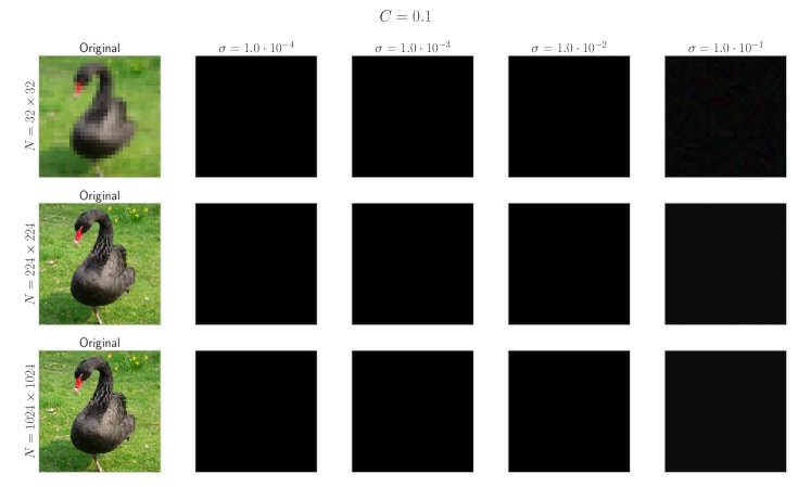
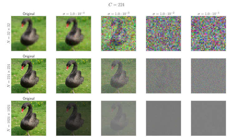
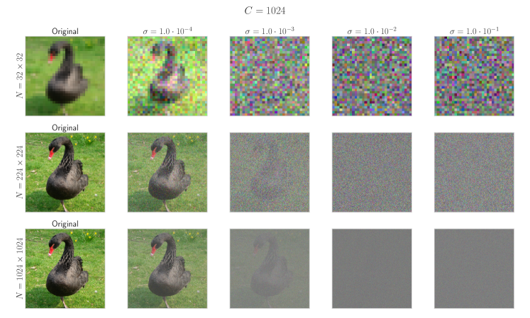
In Equation (4), we can observe a notable property of the as a reconstruction metric: The is dependent on the expected input values of , which introduces a factor scaling with the input as a bias (see Remark 2). Measuring this error is required when the exact data needs to be reconstructed. However, in other cases, such as images, where a simple prior on the value range of the data and a corresponding rescaling can make the content recognisable, this behaviour is counterproductive since scaling can result in a high error while the input can still be recognised. More concretely, a scaled will only result in a brighter or darker image, which does not indicate how well the content can be identified (see Figures 5-8 in the Appendix). The actual expected error in Equation (4) can be lower bounded independently of the input data and/or the actual clipping factor of a sample (). In Equation (5), we provide this lower bound on the expected error solely depending on the added noise and the maximum gradient norm . In Section 2.6, we extend this bound by providing the distribution of the .
2.3 Bounds on the Peak Signal-to-Noise Ratio
Since we aim to observe the relation between the true data and a scaled and noisy version of it, namely the reconstruction , we investigate the peak signal-to-noise ratio (PSNR) as a reconstruction metric.
Proposition 2.
The expected value of the between and is bounded by:
| (6) |
The derived upper bound is still dependent on the expected value range of . In the case of images, it is reasonable to assume that a data provider knows the range of pixel values, can normalise them, remove this dependency, and, by that, obtain a bound on the expected . However, in the next section, we also investigate another metric that is independent of the scaling of the image.
2.4 Bounding the Normalised Cross-Correlation
As a metric, which is independent of the linear scaling factor , we inspect the normalised cross-correlation (NCC) Rodgers and Nicewander (1988) between the input and the reconstruction .
Proposition 3.
The between the reconstruction and the actual data sample satisfies:
| (7) |
where denotes the numerically computed variance within the sample . Using , we can upper bound the as follows:
| (8) | ||||
| (9) |
We note that Equation (8) is satisfied with equality if and , for being the -dimensional vector with zeros everywhere. Also Equation (9) is an equality if additionally to the first two conditions, the data is also one-dimensional, i.e., . Comparing our two bounds, we see that the bound provided in (8) only requires the dimensionality of the data. In contrast, the bound in (9) is a fully data-independent bound, which is, however, not as tight for .
2.5 Accumulating information over multiple steps
In this section, we analyse how an adversary can boost their reconstruction performance by performing their attack multiple times.
Proposition 4.
Assuming the adversary can match queries from the same data sample, they can average the reconstructions . Thus, the following holds for the th entry of the averaged reconstructed vector
where, in this case, denotes the noise added to the th entry in the th reconstructed vector . Additionally,
| (10) |
Therefore, by performing multiple steps, the variance per coordinate decreases and the adversary is able to mitigate the privacy-preserving effects of the noise, and as a result boost their reconstruction performance.
Remark 1.
As a consequence of Proposition 4, in particular Equation (10), the estimate would converge to the (scaled) true data in samples. However, from literature Dong et al. (2022), it is known that for the Gaussian mechanism (without subsampling amplifications), the privacy measure remains constant for queries when . Hence, the effective noise scales as . Inserted into the above equation for the variance (Eq. (10)), we see that this also transfers to our results to enforce the reconstruction error remaining constant. If the sampling rate , we might have a subsampling amplification and smaller could even suffice.
| Varying | Worst-Case | Min | Max | Max | |||||
|---|---|---|---|---|---|---|---|---|---|
| Success | |||||||||
2.6 Interpreting our results in -ReRo Notation
Parallel to the analysis done in the previous sections, where we examine the expected value of different reconstruction error functions and calculate their bounds, we are also interested in determining the probability that the values of a reconstruction error function are lower than or equal to a certain threshold . Balle et al. (2022) define a mechanism to be -reconstruction robust if said probability is lower than or equal to (see definition of reconstruction robustness (ReRo), i.e., Definition 4). In the following, we describe the ReRo behaviour of the and the .
Proposition 5.
Assume the input is known. Then it follows
for a random variable with
| (11) |
where denotes the non-central chi-squared distribution with degrees of freedom and non-centrality parameter .
Proposition 6.
Once again, assume the input is known. Let be given, then for
where is the regularised gamma function. Furthermore, let be such that . Then , for
| (12) |
where denotes the chi-squared distribution with degrees of freedom.
Proposition 7.
Assume the input is known, and thus in particular, is given, then
| (13) |
for
| (14) |
and for being the regularized gamma function.
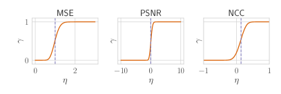
For the , the CDF can be calculated numerically. We outline the distribution in the Appendix (Eq. (68)-(79)). Analogously can be computed by calculating the CDF at . We show this in Figure 2.
3 Experiments
In this section, we demonstrate the implications of our findings through several experiments. We note that although we perform most of our experiments on image data as it is easily interpretable for humans, our attack and bounds hold for any kind of data, including tabular, language, or genetic data.
3.1 Empirical tightness evaluation
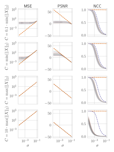
In Figure 1 we display the behaviour of the aforementioned reconstruction metrics under variation of the privacy parameters and . We see that our bounds on the and are tight when , contrary to the , which is close to the empirical results when . Both directly align with our theoretical findings: and have an introduced bias error when the gradients are clipped. The is robust to clipping but derives the bound on the variance of the data from the -norm, which is overestimated if . In addition, we see that for small clipping norms , the bound is not tight, as the data we used in this experiment is not centred. Furthermore, we observe that the clipping norm has an immediate effect on the theoretical -based bounds as well as empirical results. At the same time, the analogous to classical DP accounting models is not influenced. Hence, we see that the and bounds are tight when the gradients are not clipped, while the is robust to clipping but becomes loose if and/or , for being the -dimensional vector with zeros everywhere.
Empirically, we also observe that other reconstruction metrics, such as the normalized mutual information (NMI), structural similarity and a perceptual loss, follow similar behaviour (see Figure 1 in the Appendix). In fact, the NMI seems to have direct correspondences to the privacy parameters (see Section C.1).
3.2 Risk compared to worst-case bounds
For an informed decision on the privacy parameters, practitioners may want to consider our bounds alongside the worst-case success bound. We contrast these and explore for exemplary settings their behaviour. We consider the worst-case bound introduced by Hayes et al. (2023) and Kaissis et al. (2023a). These analyses assume an adversary who can arbitrarily modify the setting. Furthermore, they have a prior probability over a finite set of data samples containing the true data sample of choosing the correct sample randomly. The attack success is a binary outcome: either the output was successfully matched to the correct sample from the prior set or not. We note that for our bounds , as we assume an adversary without a data prior, which in the approach of Hayes et al. (2023) yields a reconstruction bound of zero, further showcasing its limited practical applicability.
In Table 1, we show for several exemplary settings the worst-case matching success rate, as well as our bounds on the , , and . We show these depending on the noise multiplier , the maximal gradient norm , the number of dimensions of the input , the number of steps and the prior probability of successful matching . We show all scenarios for a sampling rate of to make a fair comparison but note that subsampling might amplify the reconstruction bounds.
We observe that our bounds show the same trends as the worst-case bound. In particular, when increasing the noise multiplier , we see that the worst-case success converges towards the prior probability , while the increases linearly with , and the converges towards . Furthermore, all bounds display higher reconstruction success of the adversary when the number of steps increases. This behaviour can be simply counteracted by increasing (see Section 2.5).
However, the bounds show different behaviour if , or are varied. In particular, the clipping norm only influences the and bounds, which is due to the fact that the as a reconstruction metric is not robust to scaling. In fact, just by multiplying a data sample and its noisy version by the same factor, the increases linearly. Furthermore, the varies under the same parameters by changing the dimensionality of the data samples. Under the addition of the same noise and a maximum gradient norm, the decreases at higher dimensions. Lastly, the worst-case bound depends on the prior probability of a successful matching by random chance. While this consequence is obvious, the immanent question is how can be quantified in real-world scenarios.
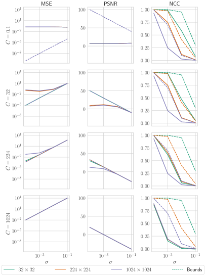
3.3 Stability of metrics with dimensions
Furthermore, we want to evaluate the influence of the dimensionality of a data sample on the reconstruction metrics. In Figure 3, we display for one image – resampled to different resolutions– the , and as reconstruction metrics. We also refer to Figures 5 - 8 in the Appendix, which show the reconstructed images. We observe that as the gradient norm increases with increasing dimensionality, we have stronger bias errors for the and at higher resolutions for small limits on the gradient norm (upper rows). At the same time, the empirical results converge to the same values across different resolutions for higher clipping norms (bottom rows). This is due to the fact that the variance of the sample remains constant as we change the resolution, yet the bound we give is based on the -norm, which increases with higher dimensionality. However, for small maximum gradient norms, the is more stable, and the deviation from the bound solely stems from the non-centred data samples. Hence, it provides further evidence that and provide tighter bounds if , i.e., the gradients are not clipped, while the is robust to clipping, but does not incorporate the influence of higher limits on the gradient norm as well.
4 Discussion and Conclusion
In this work, we formalise expectations on the reconstruction success of an adversary without prior knowledge about the data using different metrics. We now put our findings into context, especially regarding the implications of our findings on practical AI training.
We build our work on the assumption of a slightly different (and more practically relevant) threat model compared to the worst-case threat model, which has been used in similar analyses. The worst-case analysis assumes the adversary to have a finite prior set containing the target data sample. In contrast, we assume that the adversary in our scenario does not have prior knowledge about the data samples. In practice, depending on the type of data, the truth will likely lie somewhere in the middle of these assumptions. Therefore, while the worst-case bound might be too pessimistic, our results for certain cases might be too optimistic, and we thus recommend always providing them alongside worst-case bounds. We argue that the worst-case assumptions are unrealistic, as the adversary would already have access to the target point, which renders the attack pointless. However, in practical scenarios, it is not uncommon for an adversary to have access to similar data, which does not contain the exact target sample but samples from the same distribution. For example, on images, an adversary likely has access to strong data priors such as ImageNet Deng et al. (2009). This could allow them to train strong image priors, e.g., diffusion models Ho et al. (2020); Song et al. (2020), which are designed to remove noise and recover the signal from an available data sample. By doing so, the adversary could substantially increase their reconstruction success compared to our results. Bounding such attacks would be very interesting as they would likely also better correspond to the perception of humans, who themselves have strong image priors.
Depending on the concrete situation, however, our threat model could also reasonably be perceived as pessimistic as many capabilities of the adversary, in particular modifying the model architecture or loss function, can be trivially obstructed either by defining a limited set of acceptable choices or manual checks. Furthermore, in many workflows, AI models are trained on internal datasets without any external influence on the setup or observation of intermediate gradients. In such cases, adversaries can only resort to black-box reconstruction attacks, which aim to reconstruct data from the final set of weights of a trained model Haim et al. (2022); Carlini et al. (2023).
We found that the bounded metrics are complementary. While the provides bounds that are robust to scaling, these become less tight when the data is not centred. and , on the other hand, are not robust to scaling and become less tight. Furthermore, they also depend on the limit of the gradient norm, which has no influence in classical DP. One conceivable way to rid practitioners of this dependency would be to calculate the bounds at a constant sensitivity, e.g., , which leads to a situation where the metrics only depend on the noise multiplier as well as the number of steps. In the future, it would also be interesting to investigate bounds on other well-established metrics, such as the normalized mutual information (NMI), structural similarity (SSIM) or even perceptual losses. Empirically, all seem to directly correspond to the influences we observed (see Figure 4). Especially NMI seems to have a close connection to the influence of DP (see Appendix C.1). Lastly, the perceptual loss is an interesting special case, as opposed to all other metrics, it incorporates a data prior. While our bounds will not hold for adversaries with such priors, they are still obstructed as shown by the worst-case formulation.
The overarching question of providing bounds for adversarial attacks remains: how can we optimally choose the least amount of privacy in order to not introduce utility losses but still provide reasonable protection? We argue that solely investigating worst-case bounds introduces stronger privacy-utility trade-offs than necessary. Our work provides the expected risks for a certain relaxed set of assumptions and a more precise evaluation. However, we note that modifications in the assumptions might have drastic and unpredictable influence on the reconstruction risks. We see our work as a first step towards a broad suite of threat model analyses, which provides a tailored risk report for practitioners in addition to a contextualisation of how changes in the capabilities of the adversary can influence the attack success probabilities.
Software and Data
We will open-source the code used to generate all figures and tables upon acceptance of this manuscript.
Acknowledgements
We thank Johannes Kaiser and Johannes Brandt for their valuable feedback and input.
Impact Statement
This paper presents work that aims to enhance the understanding and applicability of formal privacy-preserving methods in machine learning workflows. It has many implications, and we may want to highlight the most important ones. 1) We see our work as a first step towards better understanding and formalising the risks data providers and AI practitioners face under various threat models. 2) By choosing privacy budgets that are more tailored to a specific situation, privacy-utility trade-offs are mitigated. This could help to pacify the ethical dilemma of having essential goals such as data privacy and model accuracy as competing priorities.
References
- Fowl et al. (2022) Liam Fowl, Jonas Geiping, Wojtek Czaja, Micah Goldblum, and Tom Goldstein. Robbing the fed: Directly obtaining private data in federated learning with modified models. Tenth International Conference on Learning Representations, 2022.
- Boenisch et al. (2023) Franziska Boenisch, Adam Dziedzic, Roei Schuster, Ali Shahin Shamsabadi, Ilia Shumailov, and Nicolas Papernot. When the curious abandon honesty: Federated learning is not private. In 2023 IEEE 8th European Symposium on Security and Privacy (EuroS&P), pages 175–199. IEEE, 2023.
- Song et al. (2013) Shuang Song, Kamalika Chaudhuri, and Anand D Sarwate. Stochastic gradient descent with differentially private updates. In 2013 IEEE global conference on signal and information processing, pages 245–248. IEEE, 2013.
- Abadi et al. (2016) Martin Abadi, Andy Chu, Ian Goodfellow, H Brendan McMahan, Ilya Mironov, Kunal Talwar, and Li Zhang. Deep learning with differential privacy. In Proceedings of the 2016 ACM SIGSAC conference on computer and communications security, pages 308–318, 2016.
- Guo et al. (2022) Chuan Guo, Brian Karrer, Kamalika Chaudhuri, and Laurens van der Maaten. Bounding training data reconstruction in private (deep) learning. In International Conference on Machine Learning, pages 8056–8071. PMLR, 2022.
- Balle et al. (2022) Borja Balle, Giovanni Cherubin, and Jamie Hayes. Reconstructing training data with informed adversaries. In 2022 IEEE Symposium on Security and Privacy (SP), pages 1138–1156. IEEE, 2022.
- Hayes et al. (2023) Jamie Hayes, Saeed Mahloujifar, and Borja Balle. Bounding training data reconstruction in dp-sgd. In Thirty-seventh Conference on Neural Information Processing Systems, 2023.
- Kaissis et al. (2023a) Georgios Kaissis, Jamie Hayes, Alexander Ziller, and Daniel Rueckert. Bounding data reconstruction attacks with the hypothesis testing interpretation of differential privacy. Theory and Practice of Differential Privacy, 2023a.
- Kaissis et al. (2023b) Georgios Kaissis, Alexander Ziller, Stefan Kolek, Anneliese Riess, and Daniel Rueckert. Optimal privacy guarantees for a relaxed threat model: Addressing sub-optimal adversaries in differentially private machine learning. In Thirty-seventh Conference on Neural Information Processing Systems, 2023b.
- Nasr et al. (2021) Milad Nasr, Shuang Songi, Abhradeep Thakurta, Nicolas Papernot, and Nicholas Carlini. Adversary instantiation: Lower bounds for differentially private machine learning. In 2021 IEEE Symposium on security and privacy (SP), pages 866–882. IEEE, 2021.
- Rodgers and Nicewander (1988) Joseph Lee Rodgers and W. Alan Nicewander. Thirteen ways to look at the correlation coefficient. The American Statistician, 42(1):59–66, 1988. doi: 10.1080/00031305.1988.10475524. URL https://doi.org/10.1080/00031305.1988.10475524.
- Usynin et al. (2022) Dmitrii Usynin, Daniel Rueckert, Jonathan Passerat-Palmbach, and Georgios Kaissis. Zen and the art of model adaptation: Low-utility-cost attack mitigations in collaborative machine learning. Proc. Priv. Enhancing Technol., 2022(1):274–290, 2022.
- Dong et al. (2022) Jinshuo Dong, Aaron Roth, and Weijie J Su. Gaussian differential privacy. Journal of the Royal Statistical Society Series B: Statistical Methodology, 84(1):3–37, 2022. URL https://academic.oup.com/jrsssb/article/84/1/3/7056089.
- Deng et al. (2009) Jia Deng, Wei Dong, Richard Socher, Li-Jia Li, Kai Li, and Li Fei-Fei. Imagenet: A large-scale hierarchical image database. In 2009 IEEE conference on computer vision and pattern recognition, pages 248–255. Ieee, 2009.
- Ho et al. (2020) Jonathan Ho, Ajay Jain, and Pieter Abbeel. Denoising diffusion probabilistic models. Advances in neural information processing systems, 33:6840–6851, 2020.
- Song et al. (2020) Jiaming Song, Chenlin Meng, and Stefano Ermon. Denoising diffusion implicit models. In Proceedings of the IEEE conference on computer vision and pattern recognition, pages 586–595, 2020.
- Haim et al. (2022) Niv Haim, Gal Vardi, Gilad Yehudai, Ohad Shamir, and Michal Irani. Reconstructing training data from trained neural networks. Advances in Neural Information Processing Systems, 35:22911–22924, 2022.
- Carlini et al. (2023) Nicolas Carlini, Jamie Hayes, Milad Nasr, Matthew Jagielski, Vikash Sehwag, Florian Tramer, Borja Balle, Daphne Ippolito, and Eric Wallace. Extracting training data from diffusion models. In 32nd USENIX Security Symposium (USENIX Security 23), pages 5253–5270, 2023.
- Cover (1999) Thomas M Cover. Elements of information theory. John Wiley & Sons, 1999.
- Studholme et al. (1999) Colin Studholme, Derek LG Hill, and David J Hawkes. An overlap invariant entropy measure of 3d medical image alignment. Pattern recognition, 32(1):71–86, 1999.
Appendix A Proofs
In the following, we give the proofs for our findings. See 1
Proof.
Let and be two dimensional random variables as defined in Subsection 2.1. In particular, recall that and independently drawn from . Then, we compute the by simply using its definition, as well as the linearity properties of the expectation:
| (15) | ||||
| (16) | ||||
| (17) | ||||
| (18) | ||||
| (19) | ||||
| (20) | ||||
| (21) |
Remark 2.
The results presented in Proposition 1 also align with the observation that the as we can write and by that obtain:
See 2
Proof.
Let the between and be defined as in the background section of this work (see Introduction 1). Since the logarithm with base 10 is a concave function, we can applying Jensen’s Inequality to the definition of the . If follows
| (22) | ||||
| (23) |
Then, by inserting the computed expected , see Eq. (4), we obtain an the upper bound of the expected while simultaneously making the error to be independent of the scaling factor :
| (24) | ||||
| (25) | ||||
| (26) | ||||
| (27) |
Note that in the last inequality we use the fact that minimising the expected maximises the fraction inside of the logarithm, as well as the fact that the logarithm is a non-decreasing function.
∎
See 3
Proof.
Assume and are as defined in Section 2.1. We denote the th component of and by and , respectively, for all . We let and denote the empirically computed expected value as for any coordinate of and , respectively, and use it as an estimation for and , for all . Analogously, we define and to be the empirically computed variance for any coordinate of and , where we let be shorthand notation for the standard deviation of a random variable .
First, we show Equality (7).
| (28) | |||||
| (29) | |||||
| (30) | |||||
| (31) | |||||
| (32) | |||||
| (33) | |||||
| (34) | |||||
Furthermore, we simplify :
| (35) | |||||
| (36) | |||||
| (37) | |||||
| (38) | |||||
and insert it back into the previous computation (34) of the
| (40) |
Recall, that , by definition of the variance, and that the following holds for the empirically computed :
We recall that . We used this fact in the last inequality as enforces a bound on , and it follows .
Hence,
and consequently, we can derive a bound for the expectation of :
∎
See 4
Proof.
Let , for , denote reconstructions, and represent the number of queries. Consider the average reconstructed vector :
and denote its th component by
where, in this case, denotes the noise added to the th entry in the reconstructed vector . Furthermore, since are i.i.d. for all and , with , it follows
∎
See 5
Proof.
Let us first prove , for as in Eq. (11). Let and for all . Then, we compute the as the mean error over the components:
| (41) | ||||
| (42) | ||||
| (43) | ||||
| (44) | ||||
| (45) |
where if and only if we assume that is given for all . Note that in such a scenario , for are pairwise independent. Moreover,
| (46) |
where denotes the non-central chi-squared distribution with degrees of freedom and non-centrality parameter . Thus,
for a random variable with
∎
See 6
Proof.
If we let our reconstruction error function be the , then we are interested in finding such that
Let be a random variable with
Then, by Proposition 5, it follows
| (48) | |||||
| (49) | |||||
| (50) |
To find such , we first observe the behaviour of the cumulative distribution function (CDF) of the distribution, in particular for increasing . Let , then the CDF of is given by
where denotes the Marcum -function. Since the Marcum -function is increasing in , it follows that the CDF of the distribution is decreasing in . Therefore, for a random variable and distributed as above, it holds
Thus, if
then it holds that
Since the non-central chi-squared distribution with with degrees of freedom and non-centrality parameter is the chi-squared distribution with with degrees of freedom, given we can calculate using the CDF of the distribution. Namely,
| (51) |
where denotes the regularized gamma function. Thus, (48) to (50) implies,
| (52) |
Hence, for all , and , and , such that
| (53) |
it holds
∎
See 7
Proof.
Since by definition the (see Definition 2) can be calculated using the , we can use the tools from Proposition 6 to also compute a ReRo for being the reconstruction error function. Assume is given and we want to find such that
Given , we observe the following:
| (57) | |||||
| (58) | |||||
| (59) | |||||
| (60) | |||||
| (61) |
Thus, setting
| (63) |
it follows from Proposition 6 that
| (64) | ||||
| (65) | ||||
| (66) | ||||
| (67) |
∎
Distribution of
Proposition A.1.
Let and be as defined in Section 2.1. And assume the values of and are known. The distribution of the can be calculated as
| (68) | ||||
| (69) | ||||
| (70) |
with , such that for a random variable (r.v.) with
| (71) |
Thus,
| (72) | ||||
| (73) |
with , such that , for a r.v. with
| (74) |
Hence,
| (75) |
Additionally, since
| (76) |
it follows
| (77) | ||||
| (78) |
and lastly
| (79) |
Appendix B Additional Figures
Appendix C Additional Metrics
C.1 Normalised Mutual Information
Other strategies to measure the similarity between input data and its reconstruction involve examining their entropy Cover [1999], concretely using the normalised mutual information () between them Studholme et al. [1999].
Definition C.1.
Let and be two discrete random variables. Then, the between and is given by
| (80) |
where denote the (Shannon) entropies of and , respectively, and denotes their joint entropy.
Since in our analysis we consider continuous random variables, we extend the original definition of the accordingly by using the corresponding entropy, namely the differential entropy Cover [1999].
Definition C.2.
Let and be two continuous random variables. If the differential entropies , and exist, then the between and is given by
| (81) |
Note that there are several differences between the entropy and the differential entropy, which must be considered when interpreting their values, especially since the differential entropy of a random variable can be negative Cover [1999]. These differences are highlighted in the literature on the subject of information theory.
Proposition C.1.
Let and be two continuous random variables. If the differential entropies , as well as the conditional entropy exist, then the between and is given by
| (82) |
Proof.
The assertion results from applying the chain rule to the joint entropy in the denominator of the . ∎
We inspect the extreme cases when and are independent and when is a non-randomized function of .
Intuitively, the is close to 1 when the reconstructed vector contains no information about the input, i.e. when and are independent and thus . This case takes place when the variance of the added noise is ”large enough”. However, quantifying what ”large enough” means could require making assumptions on the uncertainty of the input data distribution, which can simplify the analysis but also reduce its relevancy. Additionally, arbitrarily inflating the noise does not provide a viable solution to protecting against a reconstruction attack, since considerably increasing would also significantly decrease the model’s accuracy.
However, we still employ the normalised mutual information to assess the similarity between and under different conditions (See Figure 4). In particular, we can observe in Figure 4 that the numerical results are aligned with our intuition, namely with increasing variance of the noise , the is converges to 1.