Fair Classifiers Without Fair Training:
An Influence-Guided Data Sampling Approach

Abstract

A fair classifier should ensure the benefit of people from different groups, while the group information is often sensitive and unsuitable for model training. Therefore, learning a fair classifier but excluding sensitive attributes in the training dataset is important. In this paper, we study learning fair classifiers without implementing fair training algorithms to avoid possible leakage of sensitive information. Our theoretical analyses validate the possibility of this approach, that traditional training on a dataset with an appropriate distribution shift can reduce both the upper bound for fairness disparity and model generalization error, indicating that fairness and accuracy can be improved simultaneously with simply traditional training. We then propose a tractable solution to progressively shift the original training data during training by sampling influential data, where the sensitive attribute of new data is not accessed in sampling or used in training. Extensive experiments on real-world data demonstrate the effectiveness of our proposed algorithm.

1 Introduction

Machine Learning (ML) has dramatically impacted numerous optimization and decision-making processes across various domains, including credit scoring (Siddiqi, 2005), demand forecasting (Carbonneau et al., 2008), and healthcare (Zicari et al., 2021). Algorithmic fairness embraces the principle, often enforced by law and regulations, that the decision-maker should not exhibit biases toward protected group membership (Zhu et al., 2022), identified by characteristics such as race, gender, or disability. The literature of fairness has gained prominence to mitigate the disparities in classification tasks. In essence, the core idea of in-processing mitigation algorithms is to impose some fairness constraints during the training process, leading to a widely embraced paradigm in practice (Donini et al., 2018; Hardt et al., 2016; Agarwal et al., 2018; Zafar et al., 2017; Wang et al., 2022a; Wei et al., 2023a). However, imposing fairness constraints can introduce two challenges in the realistic settings. First, the introduced parity constraint term relies on the visibility of sensitive attributes in the training dataset, which may be inaccessible due to privacy or safety concerns (Zhu et al., 2023). Second, enforcing fairness constraints or regularizers into machine learning models often leads to a tradeoff between fairness and accuracy (Kleinberg et al., 2016), underscoring a prevalent challenge: as we place greater emphasis on ensuring fairness, the predictive model performance might be weakened. With these two concerns in mind, our core inquiry rests upon the following question:

This paper considers the following realistic scenario: we are given a large set of candidate samples without annotations. Due to the large cost of soliciting the true labels and privacy concerns of getting sensitive attributes, we are only allowed to access a small training dataset with labels and a small validation dataset with sensitive attributes. On the other hand, we are also curious about whether it is possible to learn the model without imposing any parity constraints, as constrained optimization will inevitably trade the accuracy rate and consume large computational resources. Concisely, our demand is a sampling algorithm that can effectively select a subset of training examples that suffices to mitigate the disparity without in-processing interventions.

Our proposal to address this problem is an influence-guided sampling strategy that actively samples new data points to supplement the training set. Our solution is motivated by a set of theoretical findings presented in Section 4. The analysis of the impact of data disparity on the group fairness metrics informs us that collecting new data to induce an appropriate distribution shift can effectively reduce fairness disparity without the need to implement any fair training algorithms on the updated training data.

The core challenge in crafting the sampling algorithm is approximating the influence of a candidate sample without having access to its sensitive attributes and true labels. Specifically, we assess the influence of each new unlabeled data example by comparing its gradient flow to that derived from the entire validation set, which quantifies the hypothesized change of parity metric when the specific example is included in the candidate training set. The requirement of using fairness constraints in training loss is relaxed by data sampling, as we found that the distribution shift incurred by appropriate data sampling may reduce the disparity without sacrificing model accuracy, even when the training loss does not contain any sensitive attributes. As a result, the sensitive attributes of the new unlabeled data are not required. Besides, before deciding to solicit the true label of an unlabeled example, we use the lowest-influencial label as a proxy for influence estimation. We name our solution Fair Influential Sampling (FIS).

The main contributions of our work are summarized as follows.

• Our theoretical analysis indicates that training on datasets with a strategically implemented distribution shift can effectively reduce both the upper bound for fairness disparity and model generalization error (Lemma 4.1 and Theorem 4.2). This gives us a key insight that fairness and accuracy can be improved simultaneously even with simply traditional training. [Section 4]

• We introduce a tractable solution (Algorithm 1) that progressively shifts the original training data, wherein we sample influential examples from an additional large dataset based on the combined influences of prediction and fairness without ever accessing their sensitive attributes during the training process. [Section 5]

• Empirical experiments on real-world datasets (CelebA, Adult, and COMPAS) substantiate our claims, indicating the effectiveness and potential of our proposed algorithm in achieving fairness for ML classifiers. [Section 6]

2 Related Work

Active learning. The core idea of active learning is to rank unlabeled instances by developing specific significant measures, including uncertainty (Lewis and Catlett, 1994; Lindenbaum et al., 2004), representativeness (Dasgupta and Hsu, 2008), inconsistency (Wang et al., 2012), variance (Hoi et al., 2006), and error (Roy and McCallum, 2001). Each of these measures has its own criterion to determine the importance of instances for enhancing classifier performance. For example, uncertainty considers the most important unlabeled instance to be the nearest one to the current classification boundary.

A related line of work (Liu et al., 2021a; Wang et al., 2022b; Hammoudeh and Lowd, 2022; Xie et al., 2023) concentrates on ranking unlabeled instances based on the influence function. Compared to these studies with a focus on the prediction accuracy, our work poses a distinct challenge taking into account fairness violations. We note that adopting a particular sampling strategy can lead to distribution shifts between the training and testing data. What’s worse, even though fairness is satisfied within training dataset, the model may still exhibit unfair treatments on test dataset due to the distribution shift. Therefore, it becomes imperative for the sampling approach to also account for its potential impacts on fairness.

Fair classification. The fairness-aware learning algorithms, in general, can be categorized into pre-processing, in-processing, and post-processing methods. Pre-processing methods typically reweigh or distort the data examples to mitigate the identified biases (Asudeh et al., 2019; Azzalini et al., 2021; Tae and Whang, 2021; Sharma et al., 2020; Celis et al., 2020; Chawla et al., 2002; Zemel et al., 2013; Chen et al., 2018). More relevant to us is the importance reweighting, which assigns different weights to different training examples to ensure fairness across groups (Kamiran and Calders, 2012; Jiang and Nachum, 2020; Diesendruck et al., 2020; Choi et al., 2020; Qraitem et al., 2023; Li and Vasconcelos, 2019). Our proposed algorithm bears similarity to a specific case of importance reweighting, particularly the 0-1 reweighting applied to newly added data. Other parallel studies utilize importance weighting to learn a complex fair generative model in a weakly supervised setting (Diesendruck et al., 2020; Choi et al., 2020), or to mitigate representation bias in training datasets (Li and Vasconcelos, 2019).

Post-processing methods typically enforce fairness on a learned model through calibration (Feldman, 2015; Feldman et al., 2015; Hardt et al., 2016). Although this approach can decrease the disparity of the classifier, by decoupling the training from the fairness enforcement, this procedure may not lead to the best trade-off between fairness and accuracy (Woodworth et al., 2017; Pleiss et al., 2017). In contrast, these post-processing techniques necessitate access to the sensitive attribute during the inference phase, which is often not available in many real-world scenarios.

Fairness-accuracy tradeoff. It has been demonstrated that there is an implicit trade-off between fairness and accuracy in the literature. Compared to the prior works (Menon and Williamson, 2018; Prost et al., 2019), our work does not require additional assumptions about the classifier and the characteristics of the training/testing datasets (for example, distribution shifts). Besides, the main difference is that this paper does not actually work in the classical regime of the fairness-accuracy tradeoff. By properly collecting new data from an unlabeled dataset, we can improve both generalization and fairness at the same time, which cannot be achieved by working on a fixed and static training dataset that naturally incurs such a tradeoff.

Li and Liu (2022) is a similar work that utilizes the influence function to reweight the data examples but requires re-training. Our method focuses on soliciting additional samples from an external unlabeled dataset while (Li and Liu, 2022) reweights the existing and fixed training dataset. Our approach is more closely with a fair active learning approach (Anahideh et al., 2022). However, this fair active learning framework relies on sensitive attribute information while our algorithm does not.

Distribution shifts. Common research concerning distribution shifts necessitates extra assumptions to build theoretical connections between features and attributes, like causal graphs (Singh et al., 2021), correlation shifts (Roh et al., 2023), and demographic shifts (Giguere et al., 2022). In contrast, our approach refrains from making further assumptions about the properties of distribution shifts.

In this literature, many works have utilized distributionally robust optimization (DRO) to reduce fairness disparity without sensitive attribute information (Hashimoto et al., 2018; Kirichenko et al., 2022; Liu et al., 2021b; Lahoti et al., 2020; Veldanda et al., 2023; Sohoni et al., 2020; Wei et al., 2023b). Although these works also evaluate the worst-group performance in the context of fairness, their approach differs as they do not strive to equalize the loss across all groups. Besides, in these studies, accuracy and worst-case accuracy are used to showcase the efficacy of DRO. Essentially, they equate fairness with uniform accuracy across groups, implying a model is considered fair if it demonstrates equal accuracies for all groups. However, this specific definition of fairness is somewhat restrictive and does not align with more conventional fairness definitions like DP or EOd.

3 Preliminary

3.1 Basic Scenario

We consider a standard $K$-class classification task, involving two distinct distributions: $\mathcal{P}$ for training (source) and $\mathcal{Q}$ for testing (target). Each distribution is defined as a probability distribution over certain examples, where each example, denoted as $z:=(x,y,a)$, comprises three random variables: the feature vector $x$, the label $y$, and the group membership $a$. The sensitive group $a$ often refers to characteristics such as race, gender, etc. Let $P$ and $Q$ represent the training and testing sets sampled from $\mathcal{P}$ and $\mathcal{Q}$, respectively. The training set $P$ is defined as $P:=\{(x_{n},y_{n},a_{n})\}_{n=1}^{N_{P}}$. Similarly, the test set is referred to as $Q:=\{(x_{n}^{\circ},y_{n}^{\circ},a_{n}^{\circ})\}_{n=1}^{N_{Q}}$. Note that, in practice, we are not privy to any details regarding the test dataset. Moreover, there might be potential distribution shifts between the train and test datasets, meaning that they are not independent and identically distributed (IID).

We are given a large unlabeled dataset $U:=\{(x^{\prime}_{n},\cdot,\cdot)\}_{n=1}^{N_{U}}$, which can be used for sociliting new annotations. In practice, the protected groups of datasets $P$ and $U$ remain undisclosed during training due to privacy and security concerns. The ultimate goal is to train a classifier $f$ trained on both $P$ and a small set of $U$ with a limited annotation budget for soliciting annotations while ensuring fairness constraints are satisfied on the validation dataset $Q_{v}$.

More formally, the learning objective can be formulated as

$$\min_{\mathbf{w}}\quad\frac{1}{N_{P}}\sum\nolimits_{n=1}^{N_{P}}\ell(\mathbf{w},z_{n})+\frac{1}{N_{r}}\sum\nolimits_{n=1}^{N_{r}}\ell(\mathbf{w},z_{n}^{\prime}) \quad\quad\quad\text{ s.t. }\phi(\mathbf{w},Q_{v})\leq\epsilon$$ (1)

where $\mathbf{w}$ denotes the model parameters, $N_{r}(\ll N_{U})$ represents the annotation budget, and $\ell(\mathbf{w},z)$ represents the loss function on data point $z$, which can be an indicate function $\mathbb{I}(\cdot)$ to demonstrate 0-1 loss. $\phi(\mathbf{w},Q_{v})$ indicates the fairness violation on the validation dataset $Q_{v}$ with a tolerance threshold $\epsilon$. Here, we only require the validation data with the purpose of verifying the fairness constraints are satisfied, which is IID with the test dataset $Q$.

3.2 Fairness Definition

We then introduce the concerned fairness notions:

Definition 3.1.

(Risk disparity (Hashimoto et al., 2018; Zafar et al., 2019)). Define $Q_{k}$ as the subset of $Q$ corresponding to group $k$. Given the optimized model parameters $\mathbf{w}^{P}$ trained on set $P$, the risk disparity is defined as: $\mathcal{R}_{\mathcal{Q}_{k}}(\mathbf{w}^{P})-\mathcal{R}_{\mathcal{Q}}(\mathbf{w}^{P})$, where $\mathcal{R}_{\mathcal{Q}}(\mathbf{w}):=\mathbb{E}_{z\sim\mathcal{Q}}[\ell(\mathbf{w},z)]$ denotes the expected risk induced on target distribution $\mathcal{Q}$.

Definition 3.1 highlighted in (Hashimoto et al., 2018; Zafar et al., 2019) naturally quantifies the discrepancy in a trained model’s performance between a specific group set $Q_{k}$ and the entire test set $Q$. That is, a model can be deemed fair if it exhibits consistent performance for a group set $Q_{k}$ as compared to the test dataset $Q$. Even though there may be a general incompatibility between risk disparity and popular group fairness metrics like Demographic Parity (DP) and Equalized Odds (EOd), under the criteria of this definition, these metrics could be encouraged (Shui et al., 2022; Hashimoto et al., 2018). For example, in this context, demography parity can be defined as $\sum_{k,k^{\prime}}|\mathcal{R}_{\mathcal{Q}_{k}}(\mathbf{w}^{P})-\mathcal{R}_{\mathcal{Q}_{k}^{\prime}}(\mathbf{w}^{P})|$, measuring the summation of group disparities.

Remark 3.1.

(Connections to other fairness definitions.) Definition 3.1 targets group-level fairness, which has similar granularity to the classical fairness notions such as the accuracy parity (Zafar et al., 2017), the device-level parity (Li et al., 2019), and small prediction loss for groups (Zafar et al., 2019; Balashankar et al., 2019; Martinez et al., 2019; Hashimoto et al., 2018).

4 Decoupling Fairness with Data Disparity

Including new data points to train fair classifiers raises a critical question: what strategy should we adopt to collect the data examples from the unlabeled dataset $U$ to mitigate fairness disparity without sacrificing accuracy? This task becomes particularly intricate without any further information about the training and testing data distributions, especially in the absence of sensitive attributes. In this section, we conduct a theoretical evaluation of the bounds of the risk disparity to ascertain the feasibility of our goal.

Without loss of generality, we discrete the whole distribution space and suppose that the train/test distributions are both drawn from a series of component distributions $\{\pi_{1},\cdots,\pi_{I}\}$ (Feldman, 2020). Then, the empirical risk $\mathcal{R}_{P}(\mathbf{w})$ calculated over a training set $P$ can be reformulated by splitting samples based on the component distributions:

$$\mathcal{R}_{P}(\mathbf{w}):= \mathbb{E}_{z\in P}[\ell(\mathbf{w},z)]= \sum_{i=1}^{I}p^{(P)}(\pi=i)\cdot\mathbb{E}_{z\sim\pi_{i}}[\ell(\mathbf{w},z)].$$ (2)

where $p^{(P)}(\pi=i)$ represents the frequencies of examples in $P$ drawn from component distribution $\pi_{i}$. Then, we can define the measure of probability distance between two sets or distributions as $\text{dist}(\mathcal{A},\mathcal{B}):=\sum_{i=1}^{I}|p^{(\mathcal{A})}(\pi=i)-p^{(\mathcal{B})}(\pi=i)|$.

To reflect the implicit unfairness in the models, we introduce two basic assumptions in convergence analysis (Li et al., 2019).

Assumption 4.1.

($L$-Lipschitz Continuous). There exists a constant $L>0$, for any $\mathbf{v},\mathbf{w}\in\mathbb{R}^{d}$, $\mathcal{R}_{P}(\mathbf{v})\leq\mathcal{R}_{P}(\mathbf{w})+\langle\nabla\mathcal{R}_{P}(\mathbf{w}),\mathbf{v}-\mathbf{w}\rangle+\frac{L}{2}\lVert\mathbf{v}-\mathbf{w}\rVert^{2}_{2}$.

Assumption 4.2.

(Bounded Gradient on Random Sample). The stochastic gradients on any sample $z$ are uniformly bounded, i.e., $\mathbb{E}[||\nabla\mathcal{R}_{P}(\mathbf{w}_{t},z)||^{2}]\leq G^{2}$, and training epoch $t\in[1,\cdots,T]$.

Analogous to Assumption 4.2, we further make a mild assumption to bound the loss over the component distributions $\pi_{i}$ according to the corresponding model, that is, $\mathbb{E}_{z\sim\pi_{i}}[\ell(\mathbf{w}^{P},z)]\leq G_{P},\forall i\in I$. For completeness, we first analyze the upper bound of generalization error, specifically from the standpoint of distribution shifts.

Lemma 4.1.

(Generalization error bound). Let $\text{dist}(\mathcal{P},\mathcal{Q})$, $G_{P}$ be defined therein. With probability at least $1-\delta$ with $\delta\in(0,1)$, the generalization error bound of the model trained on dataset $P$ is

$$\mathcal{R}_{\mathcal{Q}}(\mathbf{w}^{P})\leq\underbrace{G_{P}\cdot\text{dist}(\mathcal{P},\mathcal{Q})}_{\text{ distribution shift}}+\sqrt{\frac{\log(4/\delta)}{2N_{P}}}+\mathcal{R}_{P}(\mathbf{w}^{P}).$$ (3)

Note that the generalization error bound is predominantly influenced by the shift in distribution when we think of an overfitting model, i.e., the empirical risk $\mathcal{R}_{P}(\mathbf{w}^{P})\to 0$.

Theorem 4.2.

(Upper bound of risk disparity). Suppose $\mathcal{R}_{\mathcal{Q}}(\cdot)$ follows Assumption 4.1. Let $\text{dist}(\mathcal{P},\mathcal{Q})$, $G_{P}$, $\text{dist}(\mathcal{P}_{k},\mathcal{Q}_{k})$ and $\text{dist}(P_{k},P)$ be defined therein. Given model $\mathbf{w}^{P}$ and $\mathbf{w}^{k}$ trained exclusively on group $k$’s data $P_{k}$, with probability at least $1-\delta$ with $\delta\in(0,1)$, then the upper bound of the risk disparity is

$$\mathcal{R}_{\mathcal{Q}_{k}}(\mathbf{w}^{P})-\mathcal{R}_{\mathcal{Q}}(\mathbf{w}^{P})\leq G_{k}\cdot\text{dist}(\mathcal{P}_{k},\mathcal{Q}_{k})+\underbrace{G_{P}\cdot\text{dist}(\mathcal{P},\mathcal{Q})}_{\text{ distribution shift}}+\underbrace{\Phi\cdot\text{dist}(P_{k},P)^{2}}_{\text{group gap}}+\Upsilon$$ (4)

where $\Phi=4L^{2}G^{2}\sum_{t=0}^{T-1}(\eta_{t}^{2}(1+2\eta_{t}^{2}L^{2}))^{t},\Upsilon=\sqrt{\frac{\log(4/\delta)}{2N_{P}}}+\sqrt{\frac{\log(4/\delta)}{2N_{P_{k}}}}+\varpi+\varpi_{k}$.

Note that $\mathbb{E}_{z\sim\pi_{i}}[\ell(\mathbf{w}^{k},z)]\leq G_{k}$, $\varpi=\mathcal{R}_{P}(\mathbf{w}^{P})-\mathcal{R}_{\mathcal{Q}}^{*}(\mathbf{w}^{\mathcal{Q}})$ and $\varpi_{k}=\mathcal{R}_{P_{k}}(\mathbf{w}^{k})-\mathcal{R}_{\mathcal{Q}_{k}}^{*}(\mathbf{w}^{\mathcal{Q}_{k}})$. Specifically, $\varpi$ and $\varpi_{k}$ can be regarded as constants because $\mathcal{R}_{P}(\mathbf{w}^{P})$ and $\mathcal{R}_{P_{k}}(\mathbf{w}^{k})$ correspond to the empirical risks, $\mathcal{R}_{\mathcal{Q}}^{*}(\mathbf{w^{\mathcal{Q}}})$ and $\mathcal{R}_{\mathcal{Q}_{k}}^{*}(\mathbf{w^{\mathcal{Q}_{k}}})$ represent the ideal minimal empirical risk of model $\mathbf{w}^{\mathcal{Q}}$ trained on distribution $\mathcal{Q}$ and $\mathcal{Q}_{k}$, respectively.

Interpretations. The upper bound in Eq. (4) illustrates several intuitive aspects that induce unfairness. (1) Group biased data. For group-level fairness, the more balanced the data is, the smaller the risk disparity would be; (2) distribution shift. For source/target distribution, the closer the distribution is, the smaller the gap would be; (3) Data size. For training data size, the larger the size is (potentially eliminating data bias across groups), the smaller the gap would be.

Main observation. Note that Theorem 4.2 implies that the risk disparity is essentially influenced by both potential distribution shifts between the train and test datasets, as well as inherent group disparities. Our results provide guidance to reduce risk disparity by controlling the impact of distribution shifts via generalization error, which corresponds to practical model accuracy. That is, an appropriate distribution shift can reduce both the upper bound for risk disparity and generalization error. In an ideal scenario, the group gap in $P$ is smaller than the previous one in $Q$, and $\text{dist}(\mathcal{P},\mathcal{Q})$ is also small. Therefore, in general, distribution shifts typically with negative impacts on fairness can effectively be utilized to reduce the disparity without sacrificing accuracy, validating the possibility of our goal. More specifically, collecting new data pointrs to induce an appropriate distribution shift can effectively reduce disparities without the need to implement any fair training algorithms on the updated training data.

5 Improving Fairness with Data Influential Sampling

As motivated, in this section, we propose an influence-guided sampling strategy that actively solicits new data to supplement the train set, thus mitigating fairness disparity.

5.1 Finding Influential Examples

Recall that we cannot access the sensitive attribute in datasets $P$ and $U$ due to privacy concerns. The absence of sensitive attributes makes it impossible to evaluate current fairness violations and ascertain the fairness of the classifier, when we lack any knowledge about the test dataset $Q$. To overcome this limitation, we first introduce an auxiliary hold-out validation set $Q_{v}:=\{(x_{n}^{\circ},y_{n}^{\circ},a_{n}^{\circ})\}_{n=1}^{N_{v}}$, drawing from the distribution $\mathcal{Q}$ (Kirichenko et al., 2022; Liu et al., 2021b). Please note that our access is restricted solely to the sensitive attributes presented in this validation set. Despite its small size, this validation dataset offers valuable insights that aid in achieving our ultimate goal.

Inspired by recent work (Diesendruck et al., 2020; Choi et al., 2020; Li and Vasconcelos, 2019; Pruthi et al., 2020), to address the lack of sensitive attributes, the high-level idea is that we can evaluate the impact of each example on fairness by comparing the gradient originating from a single data example with the gradient derived from the entire validation set. This comparison helps in quantifying the potential advantage of including this specific example in improving fairness. Intuitively, if the gradient obtained from a single data example has a similar direction to the gradient from the validation set, it indicates that incorporating this example contributes to enhancing the model’s fairness. Similarly, the negative impact of a single data example on prediction can also be avoided by using its gradient.

In this regard, an ideal new example can help reduce the fairness disparity while keeping accuracy non-decreasing. Here, we consider the loss for the prediction component and fairness component, i.e., $\ell(\mathbf{w},z)$ and $\phi(\mathbf{w},z)$. Without loss of generality, we assume that both the loss function $\ell(\cdot)$ and fairness loss $\phi(\cdot)$ are differentiable with respect to $\mathbf{w}$ in the optimization process. Suppose that the model is updated following the gradient decent, the change of model parameters by counterfactually optimized on a new instance $z^{\prime}$ is

$$\mathbf{w}_{t+1}=\mathbf{w}_{t}-\eta\cdot\partial_{\mathbf{w}_{t}}\ell(\mathbf{w}_{t},z^{\prime})$$ (5)

where $\eta$ refers to the learning rate. Following this, we compute the influence of the prediction and fairness components, respectively.

Influence of Prediction Component. The influence for the prediction component on the validation data $z_{n}^{\circ}=(x_{n}^{\circ},y_{n}^{\circ},a_{n}^{\circ})$, when model parameters is updated from $\mathbf{w}_{t}$ to $\mathbf{w}_{t+1}$ by adding a new example $z^{\prime}$, is given by

$$\textsf{Infl}_{\textsf{acc}}(z^{\prime},z_{n}^{\circ};\mathbf{w}_{t},\mathbf{w}_{t+1}):=\ell(\mathbf{w}_{t+1},z_{n}^{\circ})-\ell(\mathbf{w}_{t},z_{n}^{\circ}).$$

For ease of notation, we use $\textsf{Infl}_{\textsf{acc}}(z^{\prime},z_{n}^{\circ})$ to represent $\textsf{Infl}_{\textsf{acc}}(z^{\prime},z_{n}^{\circ};\mathbf{w}_{t},\mathbf{w}_{t+1})$. By applying first-order Taylor expansion, we obtain the following closed-form statement:

Lemma 5.1.

The prediction influence of new example $z^{\prime}$ on the validation dataset $Q_{v}$ can be denoted by

$$\textsf{Infl}_{\textsf{acc}}(z^{\prime}):= \sum_{n\in[N_{v}]}\textsf{Infl}_{\textsf{acc}}(z^{\prime},z_{n}^{\circ})\approx -\eta\left\langle\partial_{\mathbf{w}_{t}}\ell(\mathbf{w}_{t},z^{\prime}),\sum_{n=1}^{N_{v}}\partial_{\mathbf{w}_{t}}\ell(\mathbf{w}_{t},z_{n}^{\circ})\right\rangle$$ (6)

Intuitively, the more negative $\textsf{Infl}_{\textsf{acc}}(z^{\prime})$ is, the more positive on the model prediction (performance) that example $z^{\prime}$ can provide.

Influence of Fairness Component. Recall that $\phi$ denotes the fairness loss. The fairness influence on validation data $z_{n}^{\circ}$ when model parameters change from $\mathbf{w}_{t}$ to $\mathbf{w}_{t+1}$ by adding $z^{\prime}$ is denoted by

$$\textsf{Infl}_{\textsf{fair}}(z^{\prime},z_{n}^{\circ};\mathbf{w}_{t},\mathbf{w}_{t+1}):=\phi(\mathbf{w}_{t+1},z_{n}^{\circ})-\phi(\mathbf{w}_{t},z_{n}^{\circ}).$$ (7)

For simplicity, we write $\textsf{Infl}_{\textsf{fair}}(z^{\prime},z_{n}^{\circ};\mathbf{w}_{t},\mathbf{w}_{t+1})$ as $\textsf{Infl}_{\textsf{fair}}(z^{\prime},z_{n}^{\circ})$. Then, similarly, we have

Lemma 5.2.

The fairness influence of new example $z^{\prime}$ on the validation dataset $Q_{v}$ can be denoted by

$$\textsf{Infl}_{\textsf{fair}}(z^{\prime}):= \sum_{n\in[N_{v}]}\textsf{Infl}_{\textsf{fair}}(z^{\prime},z_{n}^{\circ})\approx -\eta\sum_{n\in[N_{v}]}\left\langle\partial_{\mathbf{w}_{t}}\ell(\mathbf{w}_{t},z^{\prime}),\partial_{\mathbf{w}_{t}}\phi(\mathbf{w}_{t},z_{n}^{\circ})\right\rangle$$ (8)

Similar to the prediction component, the greater the negativity of $\textsf{Infl}_{\textsf{fair}}(z^{\prime})$ is, the greater the positive impact that the example $z^{\prime}$ has on fairness.

It is important to note that neither the influence of prediction nor fairness components require the annotations for the sensitive attributes of the sample $z^{\prime}$, which are unavailable in the dataset $U$. In contrast, calculating the first-order gradient of fairness loss $\partial_{\mathbf{w}_{t}}\phi(\mathbf{w}_{t},z_{n}^{\circ})$ only relies on the sensitive attributes of validation data $z^{\circ}$, which we assume to be available to the model learner.

We also validate how accurate the first-order estimation of the influence is in comparison to the real influence (Koh and Liang, 2017), and find that the estimated influences for most of examples are very close to their actual influence values. We refer the readers to Appendix D.3 for more details.

5.2 Algorithm: Fair Influential Sampling (FIS)

Drawing on Lemma 5.1 and Lemma 5.2, we can efficiently pinpoint those examples with the most negative fairness influence and negative prediction influence. This sampling method aids in reducing fairness disparities while sidestepping adverse impacts on accuracy.

Label Annotation. Before diving into presenting our sampling algorithm, it is necessary to address the problem of not having access to the true labels of new solicited examples. Lacking the label information for new examples poses a significant challenge in determining the corresponding influence on predictions and fairness, a fact that is substantiated by Lemma 5.1 and Lemma 5.2. In practice, one can always recruit human annotators to get the ground-truth labels for those unlabeled examples. However, we assume that it is still cost-ineffective.

To tackle this problem, one common approach is utilizing a model that has been effectively trained on dataset $P$ to produce proxy labels, which serve to approximate the calculation of influences for examples from a substantial unlabeled dataset $U$. It’s important to note that these proxy labels are exclusively used during the sampling phase. Here, we propose to annotate the proxy labels with the model trained on the labeled set $P$. In particular, we introduce a strategy that employs lowest-influence labels for the annotation of label $y^{\prime}$ given $x^{\prime}$:

$$\hat{y}=\operatorname*{arg\,min}_{k\in[K]}~{}|\textsf{Infl}_{\textsf{acc}}(x^{\prime})|,$$ (9)

which corresponds to annotating the most confident label class. After sampling, we still need to acquire the true labels of the selected data examples for subsequent training. We are aware that the true labels may not always be consistent with the elicited labels even with human annotations (Zhu et al., 2021, 2024; Cheng et al., 2020; Wei et al., 2022). The gap between human annotations and true labels is left for future works.

Algorithm 1 Fair influential sampling (FIS)

1:  Input: train set $P$, unlabeled set $U$, validation set $Q_{v}$, $t=0$, number of new examples in each round $r$, number of rounds $T$, tolerance $\epsilon$ ## Training phrase: warm start ##

2:  Train classifier $f$ solely on $P$ by minimizing the empirical risk $R_{\ell}$. Obtain model parameters $\mathbf{w}_{1}$ and validation accuracy (on $Q_{v}$) $\text{VAL}_{0}$. ## Iterative sampling phrase ##

3:  for $t$ in $\{1,2,\cdots,T\}$ do

4:     Guess label $\hat{y}$ for new examples using Eq. (9).

5:     Calculate the influence of prediction and fairness component by Eq. (6) and Eq. (8), respectively.

6:     Get the scores of fair examples:

$$S_{\text{o}}=\{\textsf{Infl}_{\textsf{fair}}(z^{\prime})~{}|~{}\textsf{Infl}_{\textsf{acc}}(z^{\prime})\leq 0,\textsf{Infl}_{\textsf{fair}}(z^{\prime})\leq 0\}$$

7:     $S_{t}=\{\}$

8:     while $|S_{t}|<r$ do

9:        Find top-$(r-|S_{t}|)$ annotated examples (lowest fairness influence):

$$\{z^{\prime}_{n}\}\leftarrow\textsf{Top-}r(S_{\text{o}})$$

10:        $S_{t}\leftarrow S_{t}\cup\{z^{\prime}_{n}~{}|~{}\textsf{Infl}_{\textsf{acc}}(z^{\prime}_{n})\leq 0,\textsf{Infl}_{\textsf{fair}}(z^{\prime}_{n})\leq 0\}$

11:     end while## Training phrase: incorporate new examples ##

12:     Train model $f$ on $P\cup S_{1}\cdots\cup S_{t}$ with true inquired labels by minimizing $R_{\ell}$. Obtain model parameters $\mathbf{w}_{t+1}$ and validation accuracy (on $Q_{v}$) $\text{VAL}_{t}-\epsilon$.

13:  end forOutput: models $\{\mathbf{w}_{t}~{}|~{}\text{VAL}_{t}>\text{VAL}_{0}\}$

Proposed algorithm. Incorporating sampling techniques, we develop a Fair Influential Sampling (FIS) method to select a limited number of influential examples from dataset $U$. The full training algorithm for fair influential sampling is summarized in Algorithm 1. Note that the tolerance $\epsilon$ is applied to monitor the performance drop in validation accuracy. In Line 2, we initiate the process by training a classifier $f$ solely on dataset $P$, that is, performing a warm start. Subsequently, T-round sampling iterations are applied to amend dataset $P$, aiming to reduce fairness disparities. Following the iterative fashion, FIS guesses labels using the proposed strategy I in Line 4. In particular, in Lines 5–6, we calculate prediction’s and fairness’s influences for examples using Lemma 5.1 and Lemma 5.2, respectively. Then, the true labels of the top-$r$ samples with the most negative impact on fairness will be inquired for further training (Lines 8-11). In Line 12, new examples will be incorporated with the training dataset $P$, followed by the continued training of the fair classifier using datapoints sampled from the updated set $P\cup S_{1}\cdots\cup S_{t}$. To amplify the influence of these new datapoints, they are assigned a greater weight compared to the datapoints in the original training dataset $P$.

Note that although we propose a specific strategy for guessing labels, our algorithm is a flexible framework that is compatible with any other labeling method. In particular, we save the model parameters at each round as checkpoints $\mathbf{w}_{t}$. Ultimately, to avoid potential accuracy drops incurred by excessively large random perturbations, we exclusively choose and offer models for output whose validation accuracy exceeds the initial validation accuracy $\text{VAL}_{0}$.

6 Empirical Results

Table 1: We report the (test_accuracy, fairness_violation) for evaluating the performance on the CelebA dataset with four binary targets, including Smiling, Attractive, Young, and Big_Nose. We select gender as the sensitive attribute.

$\epsilon=0.05$	Smiling		Attractive
	DP	EOp	DP	EOp
Base (ERM)	(0.789 ± 0.003, 0.127 ± 0.007)	(0.789 ± 0.003, 0.067 ± 0.003)	(0.664 ± 0.005, 0.251 ± 0.022)	(0.658 ± 0.009, 0.179 ± 0.014)
Random	(0.837 ± 0.017, 0.133 ± 0.001)	(0.840 ± 0.020, 0.059 ± 0.005)	(0.693 ± 0.002, 0.372 ± 0.006)	(0.693 ± 0.012, 0.250 ± 0.011)
BALD	(0.856 ± 0.024, 0.140 ± 0.012)	(0.854 ± 0.025, 0.062 ± 0.005)	(0.712 ± 0.015, 0.431 ± 0.020)	(0.712 ± 0.016, 0.297 ± 0.008)
ISAL	(0.867 ± 0.022, 0.138 ± 0.010)	(0.867 ± 0.022, 0.057 ± 0.007)	(0.713 ± 0.009, 0.410 ± 0.003)	(0.713 ± 0.009, 0.275 ± 0.011)
JTT-20	(0.698 ± 0.018, 0.077 ± 0.006)	(0.679 ± 0.013, 0.045 ± 0.002)	(0.621 ± 0.015, 0.094 ± 0.004)	(0.605 ± 0.013, 0.083 ± 0.011)
FIS	(0.848 ± 0.025, 0.084 ± 0.055)	(0.845 ± 0.034, 0.032 ± 0.007)	(0.644 ± 0.025, 0.200 ± 0.060)	(0.674 ± 0.015, 0.112 ± 0.025)
$\epsilon=0.05$	Young		Big_Nose
	DP	EOp	DP	EOp
Base(ERM)	(0.755 ± 0.002, 0.190 ± 0.017)	(0.759 ± 0.005, 0.102 ± 0.005)	(0.752 ± 0.024, 0.198 ± 0.034)	(0.755 ± 0.022, 0.206 ± 0.018)
Random	(0.763 ± 0.008, 0.158 ± 0.016)	(0.698 ± 0.109, 0.075 ± 0.021)	(0.760 ± 0.009, 0.177 ± 0.014)	(0.757 ± 0.004, 0.190 ± 0.029)
BALD	(0.776 ± 0.021, 0.165 ± 0.019)	(0.775 ± 0.020, 0.076 ± 0.007)	(0.777 ± 0.004, 0.184 ± 0.016)	(0.765 ± 0.003, 0.209 ± 0.014)
ISAL	(0.781 ± 0.020, 0.180 ± 0.014)	(0.781 ± 0.020, 0.084 ± 0.006)	(0.782 ± 0.001, 0.148 ± 0.059)	(0.782 ± 0.001, 0.154 ± 0.080)
JTT-20	(0.774 ± 0.026, 0.167 ± 0.016)	(0.774 ± 0.024, 0.083 ± 0.007)	(0.771 ± 0.014, 0.191 ± 0.036)	(0.758 ± 0.026, 0.223 ± 0.018)
FIS	(0.763 ± 0.004, 0.104 ± 0.059)	(0.773 ± 0.003, 0.041 ± 0.015)	(0.779 ± 0.009, 0.089 ± 0.076)	(0.780 ± 0.013, 0.046 ± 0.072)

In this section, we empirically demonstrate the disparate impact across groups and present the effectiveness of the proposed Fair Influential Sampling method to mitigate the disparity.

6.1 Experimental Setup

We evaluate the performance of our algorithm on four real-world datasets across three different modalities: CelebA (Liu et al., 2015), UCI Adult (Asuncion and Newman, 2007) and COMPAS (Angwin et al., 2016). We present more details about the datasets in Appendix D.1. We implement the fairness constraint $\phi(\cdot)$ using three common group fairness metrics: difference of demographic parity (DP), difference of equality of opportunity (EOp) and difference of equal odds (EOd).

We compare our method with five baselines: 1) Base (ERM): directly train the model solely on the labeled dataset $P$; 2) Random: train the model on the dataset $P$ and a subset of $Q$ by random sampling; 3) BALD (Branchaud-Charron et al., 2021): active sampling according to the mutual information; 4) ISAL (Liu et al., 2021a): selects unlabeled examples based on the calculated influence in an active learning setting. We apply model predictions as pseudo-labels. 5) Just Train Twice (JTT) (Liu et al., 2021b): reweighting those misclassified examples for retraining. Here, we examine a weight of 20 for misclassified examples, marked as JTT-20.

Recall that we present the average result of the classifier $\mathbf{w}_{t}$ outputs from Algorithm 1. Additional details on datasets and hyper-parameters are in Appendix D.

Table 2: The performance results of (test_accuracy, fairness_violation) on the Adult dataset. The selected sensitive attribute is age.

$\epsilon=0.05$	Income
	DP	EOp
Base(ERM)	(0.665 ± 0.045, 0.255 ± 0.041)	(0.665 ± 0.045, 0.115 ± 0.036)
Random	(0.765 ± 0.021, 0.209 ± 0.042)	(0.758 ± 0.027, 0.127 ± 0.013)
BALD	(0.767 ± 0.019, 0.203 ± 0.017)	(0.703 ± 0.111, 0.117 ± 0.013)
ISAL	(0.765 ± 0.020, 0.215 ± 0.011)	(0.755 ± 0.028, 0.128 ± 0.013)
JTT-20	(0.751 ± 0.013, 0.262 ± 0.020)	(0.742 ± 0.018, 0.149 ± 0.021)
FIS	(0.766 ± 0.013, 0.214 ± 0.009)	(0.757 ± 0.034, 0.113 ± 0.017)

Table 3: The performance results of (test_accuracy, fairness_violation) on the COMPAS dataset. The selected sensitive attribute is race.

$\epsilon=0.05$	Compas-Recidivism
	DP	EOp
Base (ERM)	(0.675 ± 0.005, 0.333 ± 0.008)	(0.675 ± 0.005, 0.267 ± 0.010)
Random	(0.689 ± 0.007, 0.305 ± 0.023)	(0.686 ± 0.016, 0.253 ± 0.035)
BALD	(0.688 ± 0.011, 0.313 ± 0.012)	(0.686 ± 0.015, 0.256 ± 0.031)
ISAL	(0.697 ± 0.002, 0.308 ± 0.025)	(0.698 ± 0.004, 0.274 ± 0.022)
JTT-20	(0.646 ± 0.009, 0.240 ± 0.016)	(0.630 ± 0.024, 0.141 ± 0.028)
FIS	(0.690 ± 0.002, 0.299 ± 0.029)	(0.694 ± 0.002, 0.241 ± 0.035)

6.2 Performance Results

Note that all the experimental results presented subsequently are from three separate trials, each conducted with distinct random seeds. Due to space limits, we provide a full version of the experimental results (tables) in the Appendix D.

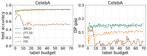
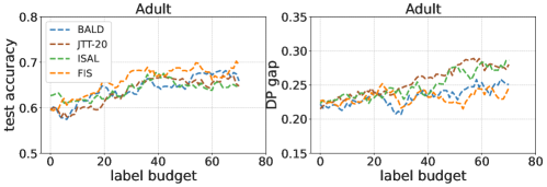
Figure 1: The impact of label budgets on the test accuracy & DP gap in the CelebA and Adult dataset, respectively. The binary classification target is Smiling for the CelebA dataset.

Results on image datasets. Initially, we train a vision transformer using a patch size of $(8,8)$ on the CelebA face attribute dataset (Liu et al., 2015). We select four binary classification targets, including Smiling, Attractive, Young, and Big Nose. The sensitive attribute is gender. 2% of the labeled data is allocated for training, while the remaining 98% is reserved for sampling purposes. Then, 10% of the test data is randomly set aside as a hold-out validation set. For ease of computation, only the last two layers of the model are used to calculate the influence of prediction and fairness components. Table 1 report the obtained accuracy and the corresponding values of fairness metrics. One main observation is that our proposed method FIS outperforms baselines with a significant margin on three fairness metrics, while maintaining the same accuracy level. This improvement, as indicated by our findings in Theorem 4.2, can be attributed to FIS assigning priority to new examples based on the influence of fairness, thus averting potential accuracy reduction by assessing the corresponding influence of prediction.

Results on tabular datasets. Next, we work with multi-layer perceptron (MLP) with two layers trained on the Adult dataset (Asuncion and Newman, 2007) and Compas dataset (Angwin et al., 2016), respectively. We select age as the sensitive attribute for the Adult dataset and race for the COMPAS dataset. For both of the datasets, we resample the data to balance the class and group membership (Chawla et al., 2002). We randomly split the whole dataset into a training and a test set in a ratio of 80 to 20. Then, we randomly re-select 20% of the training set for initial training and the remaining 80% for sampling. Also, 20% examples of the test set are selected to form a validation set. The MLP model is a two-layer ReLU network with a hidden size of 64. We utilize the whole model parameters to compute the influence of prediction and fairness for examples. Table 2 and Table 3 summarize the key results of the Adult and Compas datasets, respectively. On Adult dataset, we observe that our sampling method achieves the lowest violation for equality of opportunity and has a comparable performance for the demographic parity metric. Besides, our algorithm achieves a much better accuracy-fairness trade-off than the other compared methods on the COMPAS dataset. Though the JTT-20 method indeed has a lower fairness violation, we highlight that they suffer from a dramastic accuracy drop than the other baselines.

6.3 Impact of Label Budgets

We conduct an ablation study to examine how the varying label budgets $r$ affects the trade-off between accuracy and fairness. For ease of comparison, we adhere to a consistent label budget per round to illustrate their respective impacts. As shown in Figure 1, our method consistently preserves a lower fairness violation than the BALD and ISAL baselines with a similar test accuracy. While we observe that the JTT-20 algorithm is able to achieve a near-zero fairness violation under a limited budget on the CelebA dataset, we argue that the prediction accuracy is rather uninformative (about 50%). Conversely, on the Adult dataset, both accuracy and fairness violation converge to similar numerical values when the budget is lower than 20, suggesting a potential overfitting of the model to insufficient training examples. With a larger budget, our algorithms outperform other baseline methods, achieving higher accuracy and lower demographic disparity. We defer more experiment details in the Appendix D.3.

7 Concluding Remarks

In this work, we explore the training of fair classifiers without imposing fairness constraints, aiming to prevent the potential exposure of sensitive attributes. Our theoretical finding affirms that by using traditional training on suitably shifted dataset distributions, we can decrease the bounds of fairness disparity and model generalization error simultaneously. Motivated by the insights from our results, we propose a fair influential sampling method FIS to inquiry data samples from a large unlabeled dataset to progressively shift the original training data during training. Importantly, the sensitive attribute of new examples is neither accessed during sampling nor used in the training phase. The privilege of our method is that we acquire the data examples that may cause negative impacts on the fairness violations during the sampling process. Excluding these specific data examples during training is likely to contribute to mitigating unfairness at test time. Empirical experiments on real-world data validate the efficacy of our proposed method.

Nonetheless, we recognize that our method has limitations. Although the proposed sampling algorithm does not require the sensitive attribute information from the massive unlabeled data, it relies on a clean and informative validation set which contains the sensitive attributes of data examples. We consider this as a reasonable requirement in practice, given the relatively modest size of the validation set.

Appendix

Appendix A More Details of Related Work

Active learning. The core idea of active learning is to rank unlabeled instances by developing specific significant measures, including uncertainty [Lewis and Catlett, 1994, Lindenbaum et al., 2004], representativeness [Dasgupta and Hsu, 2008], inconsistency [Wang et al., 2012], variance [Hoi et al., 2006], and error [Roy and McCallum, 2001]. Each of these measures has its own criterion to determine the importance of instances for enhancing classifier performance. For example, uncertainty considers the most important unlabeled instance to be the nearest one to the current classification boundary.

A related line of work [Liu et al., 2021a, Wang et al., 2022b, Hammoudeh and Lowd, 2022, Xie et al., 2023] concentrates on ranking unlabeled instances based on the influence function. Compared to these studies with a focus on the prediction accuracy, our work poses a distinct challenge taking into account fairness violations. We note that adopting a particular sampling strategy can lead to distribution shifts between the training and testing data. What’s worse, even though fairness is satisfied within training dataset, the model may still exhibit unfair treatments on test dataset due to the distribution shift. Therefore, it becomes imperative for the sampling approach to also account for its potential impacts on fairness.

Fair classification. The fairness-aware learning algorithms, in general, can be categorized into pre-processing, in-processing, and post-processing methods. Pre-processing methods typically reweigh or distort the data examples to mitigate the identified biases [Asudeh et al., 2019, Azzalini et al., 2021, Tae and Whang, 2021, Sharma et al., 2020, Celis et al., 2020, Chawla et al., 2002, Zemel et al., 2013, Chen et al., 2018]. More relevant to us is the importance reweighting, which assigns different weights to different training examples to ensure fairness across groups [Kamiran and Calders, 2012, Jiang and Nachum, 2020, Diesendruck et al., 2020, Choi et al., 2020, Qraitem et al., 2023, Li and Vasconcelos, 2019]. Our proposed algorithm bears similarity to a specific case of importance reweighting, particularly the 0-1 reweighting applied to newly added data. The main advantage of our work, however, lies in its ability to operate without needing access to the sensitive attributes of either the new or training data. Other parallel studies utilize importance weighting to learn a complex fair generative model in a weakly supervised setting [Diesendruck et al., 2020, Choi et al., 2020], or to mitigate representation bias in training datasets [Li and Vasconcelos, 2019].

Post-processing methods typically enforce fairness on a learned model through calibration [Feldman, 2015, Feldman et al., 2015, Hardt et al., 2016]. Although this approach is likely to decrease the disparity of the classifier, by decoupling the training from the fairness enforcement, this procedure may not lead to the best trade-off between fairness and accuracy [Woodworth et al., 2017, Pleiss et al., 2017]. In contrast, our work can achieve a better trade-off between fairness and accuracy, because we reduce the fairness disparity by mitigating the adverse effects of distribution shifts on generalization error. Additionally, these post-processing techniques necessitate access to the sensitive attribute during the inference phase, which is often not available in many real-world scenarios.

Fairness-accuracy tradeoff. It has been demonstrated that there is an implicit trade-off between fairness and accuracy in the literature. Compared to the prior works [Menon and Williamson, 2018, Prost et al., 2019], our work does not require additional assumptions about the classifier and the characteristics of the training/testing datasets (for example, distribution shifts). Besides, the main difference is that this paper does not actually work in the classical regime of the fairness-accuracy tradeoff. By properly collecting new data from an unlabeled dataset, we can improve both generalization and fairness at the same time, which cannot be achieved by working on a fixed and static training dataset that naturally incurs such a tradeoff.

Li and Liu [2022] is a similar work that utilizes the influence function to reweight the data examples but requires re-training. Our method focuses on soliciting additional samples from an external unlabeled dataset while [Li and Liu, 2022] reweights the existing and fixed training dataset. Our approach is more closely with a fair active learning approach [Anahideh et al., 2022]. However, this fair active learning framework relies on sensitive attribute information while our algorithm does not.

Distribution shifts. Common research concerning distribution shifts necessitates extra assumptions to build theoretical connections between features and attributes, like causal graphs [Singh et al., 2021], correlation shifts [Roh et al., 2023], and demographic shifts [Giguere et al., 2022]. In contrast, our approach refrains from making further assumptions about the properties of distribution shifts.

In this literature, many works have utilized distributionally robust optimization (DRO) to reduce fairness disparity without sensitive attribute information [Hashimoto et al., 2018, Kirichenko et al., 2022, Liu et al., 2021b, Lahoti et al., 2020, Veldanda et al., 2023, Sohoni et al., 2020, Wei et al., 2023b]. Although these works also evaluate the worst-group performance in the context of fairness, their approach differs as they do not strive to equalize the loss across all groups. Besides, in these studies, accuracy and worst-case accuracy are used to showcase the efficacy of DRO. Essentially, they equate fairness with uniform accuracy across groups, implying a model is considered fair if it demonstrates equal accuracies for all groups. However, this specific definition of fairness is somewhat restrictive and does not align with more conventional fairness definitions like DP or EOd.

Appendix B Omitted Proofs

In this section, we present detailed proofs for the lemmas and theorems in Sections 4 and 5, respectively.

B.1 Proof of Lemma 4.1

Lemma B.1.

(Generalization error bound). Let $\text{dist}(\mathcal{P},\mathcal{Q})$, $G_{P}$ be defined therein. With probability at least $1-\delta$ with $\delta\in(0,1)$, the generalization error bound of the model trained on dataset $P$ is

$$\mathcal{R}_{\mathcal{Q}}(\mathbf{w}^{P})\leq\underbrace{G_{P}\cdot\text{dist}(\mathcal{P},\mathcal{Q})}_{\text{ distribution shift}}+\sqrt{\frac{\log(4/\delta)}{2N_{P}}}+\mathcal{R}_{P}(\mathbf{w}^{P}).$$ (10)

Note that the generalization error bound is predominantly influenced by the shift in distribution when we think of an overfitting model, i.e., the empirical risk $\mathcal{R}_{P}(\mathbf{w}^{P})\to 0$. The detailed proof is presented as follows.

Proof.

The generalization error bound is

$$\begin{split}\mathcal{R}_{\mathcal{Q}}(\mathbf{w}^{P})&=\underbrace{\bigg{(}\mathcal{R}_{\mathcal{Q}}(\mathbf{w}^{P})-\mathcal{R}_{\mathcal{P}}(\mathbf{w}^{P})\bigg{)}}_{\text{distribution shift}}+\underbrace{\bigg{(}\mathcal{R}_{\mathcal{P}}(\mathbf{w}^{P})-\mathcal{R}_{P}(\mathbf{w}^{P})\bigg{)}}_{\text{Hoeffding's inequality}}+\underbrace{\mathcal{R}_{P}(\mathbf{w}^{P}))}_{\text{empirical risk}}\\ &\leq G_{P}\cdot\text{dist}(\mathcal{P},\mathcal{Q})+\sqrt{\frac{\log(4/\delta)}{2N_{P}}}+\mathcal{R}_{P}(\mathbf{w}^{P})\\ \end{split}$$

For the first term (distribution shift), we have

$$\begin{split}\mathcal{R}_{\mathcal{Q}}(\mathbf{w}^{P})-\mathcal{R}_{\mathcal{P}}(\mathbf{w}^{P})&=\mathbb{E}_{z\sim\mathcal{Q}}[\ell(\mathbf{w}^{P},z)]-\mathbb{E}_{z\sim\mathcal{P}}[\ell(\mathbf{w}^{P},z)]\\ &=\sum_{i=1}^{I}p^{(\mathcal{Q})}(\pi=i)\mathbb{E}_{z\sim\pi_{i}}[\ell(\mathbf{w}^{P},z)]-\sum_{i=1}^{I}p^{(\mathcal{P})}(\pi=i)\mathbb{E}_{z\sim\pi_{i}}[\ell(\mathbf{w}^{P},z)]\\ &=\sum_{i=1}^{I}|p^{(\mathcal{P})}(\pi=i)-p^{(\mathcal{Q})}(\pi=i)|\mathbb{E}_{z\sim\pi_{i}}[\ell(\mathbf{w}^{P},z)]\\ &\leq G_{P}\cdot\text{dist}(\mathcal{P},\mathcal{Q}).\end{split}$$

where we define $\text{dist}(\mathcal{P},\mathcal{Q})=\sum_{i=1}^{I}|p^{(\mathcal{P})}(\pi=i)-p^{(\mathcal{Q})}(\pi=i)|$ and $\mathbb{E}_{z\sim\pi_{i}}[\ell(\mathbf{w}^{P},z)]\leq G_{P},\forall i\in I$ because of Assumption 4.2. To avoid misunderstanding, we use a subscript $P$ of the constant $G$ to clarify the corresponding model $\mathbf{w}^{P}$. Then, for the second term (Hoeffding inequality), with probability at least $1-\delta$, we have $|\mathcal{R}_{\mathcal{P}}(\mathbf{w}^{P})-\mathcal{R}_{P}(\mathbf{w}^{P})|\leq\sqrt{\frac{\log(4/\delta)}{2N_{P}}}$. ∎

B.2 Proof of Theorem 4.2

Theorem 4.2. (Upper bound of fairness disparity). Suppose $\mathcal{R}_{\mathcal{Q}}(\cdot)$ follows Assumption 4.1. Let $\text{dist}(\mathcal{P},\mathcal{Q})$, $G_{P}$, $\text{dist}(\mathcal{P}_{k},\mathcal{Q}_{k})$ and $\text{dist}(P_{k},P)$ be defined therein. Given model $\mathbf{w}^{P}$ and $\mathbf{w}^{k}$ trained exclusively on group $k$’s data $P_{k}$, with probability at least $1-\delta$ with $\delta\in(0,1)$, then the upper bound of the fairness disparity is

$$\begin{split}\mathcal{R}_{\mathcal{Q}_{k}}(\mathbf{w}^{P})-\mathcal{R}_{\mathcal{Q}}(\mathbf{w}^{P})\leq\underbrace{G_{P}\cdot\text{dist}(\mathcal{P},\mathcal{Q})}_{\text{ distribution shift}}+\underbrace{\Phi\cdot\text{dist}(P_{k},P)^{2}}_{\text{group gap}}+G_{k}\cdot\text{dist}(\mathcal{P}_{k},\mathcal{Q}_{k})+\Upsilon.\end{split}$$

where

$$\Phi=4L^{2}G^{2}\sum_{t=0}^{T-1}(\eta_{t}^{2}(1+2\eta_{t}^{2}L^{2}))^{t},\quad\Upsilon=\sqrt{\frac{\log(4/\delta)}{2N_{P}}}+\sqrt{\frac{\log(4/\delta)}{2N_{P_{k}}}}+\varpi+\varpi_{k}$$

Note that $\mathbb{E}_{z\sim\pi_{i}}[\ell(\mathbf{w}^{k},z)]\leq G_{k}$, $\varpi=\mathcal{R}_{P}(\mathbf{w}^{P})-\mathcal{R}_{\mathcal{Q}}^{*}(\mathbf{w}^{\mathcal{Q}})$ and $\varpi_{k}=\mathcal{R}_{P_{k}}(\mathbf{w}^{k})-\mathcal{R}_{\mathcal{Q}_{k}}^{*}(\mathbf{w}^{\mathcal{Q}_{k}})$. Specifically, $\varpi$ and $\varpi_{k}$ can be regarded as constants because $\mathcal{R}_{P}(\mathbf{w}^{P})$ and $\mathcal{R}_{P_{k}}(\mathbf{w}^{k})$ correspond to the empirical risks, $\mathcal{R}_{\mathcal{Q}}^{*}(\mathbf{w^{\mathcal{Q}}})$ and $\mathcal{R}_{\mathcal{Q}_{k}}^{*}(\mathbf{w^{\mathcal{Q}_{k}}})$ represent the ideal minimal empirical risk of model $\mathbf{w}^{\mathcal{Q}}$ trained on distribution $\mathcal{Q}$ and $\mathcal{Q}_{k}$, respectively.

Proof.

First of all, we have

$$\mathcal{R}_{\mathcal{Q}_{k}}(\mathbf{w}^{P})-\mathcal{R}_{\mathcal{Q}}(\mathbf{w}^{P}) =(\mathcal{R}_{\mathcal{Q}}(\mathbf{w}^{P_{k}})-\mathcal{R}_{\mathcal{Q}}(\mathbf{w}^{P}))+(\mathcal{R}_{\mathcal{Q}_{k}}(\mathbf{w}^{P})-\mathcal{R}_{\mathcal{Q}}(\mathbf{w}^{P_{k}}))$$

$$=(\mathcal{R}_{\mathcal{Q}}(\mathbf{w}^{P_{k}})-\mathcal{R}_{\mathcal{Q}}(\mathbf{w}^{P}))+(\mathcal{R}_{\mathcal{Q}_{k}}(\mathbf{w}^{P})-\mathcal{R}_{\mathcal{Q}_{k}}(\mathbf{w}^{P_{k}}))+(\mathcal{R}_{\mathcal{Q}_{k}}(\mathbf{w}^{P_{k}})-\mathcal{R}_{\mathcal{Q}}(\mathbf{w}^{P_{k}}))$$

$$\leq(\mathcal{R}_{\mathcal{Q}}(\mathbf{w}^{P_{k}})-\mathcal{R}_{\mathcal{Q}}(\mathbf{w}^{P}))+(\mathcal{R}_{\mathcal{Q}_{k}}(\mathbf{w}^{P})-\mathcal{R}_{\mathcal{Q}_{k}}(\mathbf{w}^{P_{k}}))$$

where $\mathbf{w}^{P_{k}}$ represents the model trained exclusively on group $k$’s data. For simplicity, when there is no confusion, we use $\mathbf{w}^{k}$ to substitute $\mathbf{w}^{P_{k}}$. The inequality $\mathcal{R}_{\mathcal{Q}_{k}}(\mathbf{w}^{k})-\mathcal{R}_{\mathcal{Q}}(\mathbf{w}^{k})\leq 0$ holds due to the fact that the model tailored for a single group $k$ can not generalize well to the entirety of the test set $Q$.

Then, for the first term, we have

$$\begin{split}\mathcal{R}_{\mathcal{Q}}(\mathbf{w}^{k})-\mathcal{R}_{\mathcal{Q}}(\mathbf{w}^{P})&\stackrel{{\scriptstyle(a)}}{{\leq}}\langle\nabla\mathcal{R}_{\mathcal{Q}}(\mathbf{w}^{P}),\mathbf{w}^{k}-\mathbf{w}^{P}\rangle+\frac{L}{2}\lVert\mathbf{w}^{k}-\mathbf{w}^{P}\rVert^{2}\\ &\stackrel{{\scriptstyle(b)}}{{\leq}}L\lVert\mathbf{w}^{k}-\mathbf{w}^{P}\rVert^{2}+\frac{1}{2L}\lVert\nabla\mathcal{R}_{\mathcal{Q}}(\mathbf{w}^{P})\rVert^{2}\\ &\stackrel{{\scriptstyle(c)}}{{\leq}}\underbrace{L\lVert\mathbf{w}^{k}-\mathbf{w}^{P}\rVert^{2}}_{\text{group gap}}+\underbrace{(\mathcal{R}_{\mathcal{Q}}(\mathbf{w}^{P})-\mathcal{R}_{\mathcal{Q}}^{*}(\mathbf{w^{\mathcal{Q}}}))}_{\text{train-test model gap}}\end{split}$$

where inequality (a) holds because of the L-smoothness of expected loss $\mathcal{R}_{\mathcal{Q}}(\cdot)$, i.e., Assumption 4.1. Specifically, inequality (b) holds because, by Cauchy-Schwarz inequality and AM-GM inequality, we have

$$\langle\nabla\mathcal{R}_{\mathcal{Q}}(\mathbf{w}^{P}),\mathbf{w}^{k}-\mathbf{w}^{P}\rangle\leq\frac{L}{2}\lVert\mathbf{w}^{k}-\mathbf{w}^{P}\rVert^{2}+\frac{1}{2L}\lVert\nabla\mathcal{R}_{\mathcal{Q}}(\mathbf{w}^{P})\rVert^{2}.$$

Then, inequality (c) holds due to the L-smoothness of $\mathcal{R}_{\mathcal{Q}}(\cdot)$ (Assumption 4.1), we can get a variant of Polak-Łojasiewicz inequality, which follows

$$\lVert\nabla\mathcal{R}_{\mathcal{Q}}(\mathbf{w}^{P})\rVert^{2}\leq 2L(\mathcal{R}_{\mathcal{Q}}(\mathbf{w}^{P})-\mathcal{R}_{\mathcal{Q}}^{*}(\mathbf{w^{\mathcal{Q}}})).$$

Following a similar idea, for the second term, we also have

$$\begin{split}\mathcal{R}_{\mathcal{Q}_{k}}(\mathbf{w}^{P})-\mathcal{R}_{\mathcal{Q}_{k}}(\mathbf{w}^{k})&\leq L\lVert\mathbf{w}^{P}-\mathbf{w}^{k}\rVert^{2}+(\mathcal{R}_{\mathcal{Q}_{k}}(\mathbf{w}^{k})-\mathcal{R}_{\mathcal{Q}_{k}}^{*}(\mathbf{w}^{\mathcal{Q}_{k}}))\end{split}$$

Combined with two terms, we have

$$\mathcal{R}_{\mathcal{Q}_{k}}(\mathbf{w}^{P})-\mathcal{R}_{\mathcal{Q}}(\mathbf{w}^{P}) \leq\underbrace{(\mathcal{R}_{\mathcal{Q}}(\mathbf{w}^{P})-\mathcal{R}_{\mathcal{Q}}^{*}(\mathbf{w^{\mathcal{Q}}}))}_{\text{train-test model gap}}+\underbrace{2L\lVert\mathbf{w}^{k}-\mathbf{w}^{P}\rVert^{2}}_{\text{group gap}}+(\mathcal{R}_{\mathcal{Q}_{k}}(\mathbf{w}^{k})-\mathcal{R}_{\mathcal{Q}_{k}}^{*}(\mathbf{w}^{\mathcal{Q}_{k}}))$$

Lastly, integrating with Lemma B.2, B.3 and B.4, we can finish the proof. ∎

Lemma B.2.

(Train-test model gap) With probability at least $1-\delta$, given the model $\mathbf{w}^{P}$ trained on train set $P$, we have

$$\mathcal{R}_{\mathcal{Q}}(\mathbf{w}^{P})-\mathcal{R}_{\mathcal{Q}}^{*}(\mathbf{w^{\mathcal{Q}}})\leq G_{P}\cdot\text{dist}(\mathcal{P},\mathcal{Q})+\sqrt{\frac{\log(4/\delta)}{2N_{P}}}+\varpi.$$

where $\text{dist}(\mathcal{P},\mathcal{Q})=\sum_{i=1}^{I}|p^{(\mathcal{P})}(\pi=i)-p^{(\mathcal{Q})}(\pi=i)|$ and $\mathbb{E}_{z\sim\pi_{i}}[\ell(\mathbf{w}^{P},z)]\leq G_{P},\forall i\in I$, and a constant $\varpi:=\mathcal{R}_{P}(\mathbf{w}^{P})-\mathcal{R}_{\mathcal{Q}}^{*}(\mathbf{w^{\mathcal{Q}}})$.

Proof.

First of all, we have,

$$\begin{split}\mathcal{R}_{\mathcal{Q}}(\mathbf{w}^{P})-\mathcal{R}_{\mathcal{Q}}^{*}(\mathbf{w^{\mathcal{Q}}})&=\bigg{(}\mathcal{R}_{\mathcal{Q}}(\mathbf{w}^{P})-\mathcal{R}_{\mathcal{P}}(\mathbf{w}^{P})\bigg{)}+\mathcal{R}_{\mathcal{P}}(\mathbf{w}^{P})-\mathcal{R}_{\mathcal{Q}}^{*}(\mathbf{w^{\mathcal{Q}}})\\ &\leq G\cdot\text{dist}(\mathcal{P},\mathcal{Q})+\mathcal{R}_{\mathcal{P}}(\mathbf{w}^{P})-\mathcal{R}_{\mathcal{Q}}^{*}(\mathbf{w^{\mathcal{Q}}})\\ &\leq\underbrace{G\cdot\text{dist}(\mathcal{P},\mathcal{Q})}_{\text{distribution shift}}+\underbrace{\bigg{(}\mathcal{R}_{\mathcal{P}}(\mathbf{w}^{P})-\mathcal{R}_{P}(\mathbf{w}^{P})\bigg{)}}_{\text{Hoeffding's inequality}}+\underbrace{\bigg{(}\mathcal{R}_{P}(\mathbf{w}^{P})-\mathcal{R}_{\mathcal{Q}}^{*}(\mathbf{w^{\mathcal{Q}}})\bigg{)}}_{\text{overfitting \& ideal case}}\\ \end{split}$$

For the first term (distribution shift), we have

$$\begin{split}\mathcal{R}_{\mathcal{Q}}(\mathbf{w}^{P})-\mathcal{R}_{\mathcal{P}}(\mathbf{w}^{P})&=\mathbb{E}_{z\sim\mathcal{Q}}[\ell(\mathbf{w}^{P},z)]-\mathbb{E}_{z\sim\mathcal{P}}[\ell(\mathbf{w}^{P},z)]\\ &=\sum_{i=1}^{I}p^{(\mathcal{Q})}(\pi=i)\mathbb{E}_{z\sim\pi_{i}}[\ell(\mathbf{w}^{P},z)]-\sum_{i=1}^{I}p^{(\mathcal{P})}(\pi=i)\mathbb{E}_{z\sim\pi_{i}}[\ell(\mathbf{w}^{P},z)]\\ &\leq\sum_{i=1}^{I}|p^{(\mathcal{P})}(\pi=i)-p^{(\mathcal{Q})}(\pi=i)|\mathbb{E}_{z\sim\pi_{i}}[\ell(\mathbf{w}^{P},z)]\\ &\leq G_{P}\cdot\text{dist}(\mathcal{P},\mathcal{Q}).\end{split}$$

where we define $\text{dist}(\mathcal{P},\mathcal{Q})=\sum_{i=1}^{I}|p^{(\mathcal{P})}(\pi=i)-p^{(\mathcal{Q})}(\pi=i)|$ and $\mathbb{E}_{z\sim\pi_{i}}[\ell(\mathbf{w}^{P},z)]\leq G_{P},\forall i\in I$ because of Assumption 4.2. For the second term, with probability at least $1-\delta$, we have $|\mathcal{R}_{\mathcal{P}}(\mathbf{w}^{P})-\mathcal{R}_{P}(\mathbf{w}^{P})|\leq\sqrt{\frac{\log(4/\delta)}{2N_{P}}}$. Note that the third term $\mathcal{R}_{P}(\mathbf{w}^{P})-\mathcal{R}_{Q}^{*}(\mathbf{w^{\mathcal{Q}}})$ can be regarded as a constant $\varpi$.because $\mathcal{R}_{P}(\mathbf{w}^{P})$ is the empirical risk and $\mathcal{R}_{\mathcal{Q}}^{*}(\mathbf{w^{\mathcal{Q}}})$ is the ideal minimal empirical risk of model $\mathbf{w}^{\mathcal{Q}}$ trained on distribution $\mathcal{Q}$.

Therefore, with probability at least $1-\delta$, given model $\mathbf{w}^{P}$,

$$\mathcal{R}_{\mathcal{Q}}(\mathbf{w}^{P})-\mathcal{R}_{\mathcal{Q}}^{*}(\mathbf{w^{\mathcal{Q}}})\leq G_{P}\cdot\text{dist}(\mathcal{P},\mathcal{Q})+\sqrt{\frac{\log(4/\delta)}{2N_{P}}}+\varpi.$$

∎

Lemma B.3.

(Group gap) Suppose Assumptions 4.1 and 4.2 hold for empirical risk $\mathcal{R}_{P}(\cdot)$, then we have

$$\lVert\mathbf{w}^{k}-\mathbf{w}^{P}\rVert^{2}\leq 2LG^{2}\sum_{t=0}^{T}(\eta_{t}^{2}(1+2\eta_{t}^{2}L^{2}))^{t}\bigg{(}\sum_{i=1}^{I}\bigg{|}p^{(k)}(\pi=i)-p^{(P)}(\pi=i)\bigg{|}\bigg{)}^{2}.$$

where $\eta_{t}$ is epoch $t$’s learning rate and T is the number of epochs.

Proof.

According to the above definition, we similarly define the following empirical risk $\mathcal{R}_{P_{k}}(\mathbf{w})$ over group $k$’s data $P_{k}$ by splitting samples according to their marginal distributions, shown as follows.

$$\mathcal{R}_{P_{k}}(\mathbf{w}):=\sum_{i=1}^{I}p^{(k)}(\pi=i)\mathbb{E}_{z\sim\pi_{i}}[\ell(\mathbf{w},z)].$$

Let $\eta_{t}$ indicate the learning rate of epoch $t$. Then, for each epoch $t$, group $k$’s optimizer performs SGD as follows:

$$\mathbf{w}_{t}^{k}=\mathbf{w}_{t-1}^{k}-\eta_{t}\sum_{i=1}^{I}p^{(k)}(\pi=i)\nabla_{\mathbf{w}}\mathbb{E}_{z\sim\pi_{i}}[\ell(\mathbf{w}_{t-1}^{k},z)].$$

For any epoch $t+1$, we have

$$\begin{split}&\lVert\mathbf{w}^{k}_{t+1}-\mathbf{w}^{P}_{t+1}\rVert^{2}\\ &=\lVert\mathbf{w}^{k}_{t}-\eta_{t}\sum_{i=1}^{I}p^{(k)}(\pi=i)\nabla_{\mathbf{w}}\mathbb{E}_{z\sim\pi_{i}}[\ell(\mathbf{w}_{t}^{k},z)]-\mathbf{w}^{P}_{t}+\eta_{t}\sum_{i=1}^{I}p^{(P)}(\pi=i)\nabla_{\mathbf{w}}\mathbb{E}_{z\sim\pi_{i}}[\ell(\mathbf{w}_{t}^{P},z)]\rVert^{2}\\ &\leq\lVert\mathbf{w}^{k}_{t}-\mathbf{w}^{P}_{t}\rVert^{2}+\eta_{t}^{2}\lVert\sum_{i=1}^{I}p^{(k)}(\pi=i)\nabla_{\mathbf{w}}\mathbb{E}_{z\sim\pi_{i}}[\ell(\mathbf{w}_{t}^{k},z)]-\sum_{i=1}^{I}p^{(P)}(\pi=i)\nabla_{\mathbf{w}}\mathbb{E}_{z\sim\pi_{i}}[\ell(\mathbf{w}_{t}^{P},z)]\rVert^{2}\\ &\leq\lVert\mathbf{w}^{k}_{t}-\mathbf{w}^{P}_{t}\rVert^{2}+2\eta_{t}^{2}\lVert\sum_{i=1}^{I}p^{(P)}(\pi=i)L_{\pi_{i}}\bigg{[}\nabla_{\mathbf{w}}\mathbb{E}_{z\sim\pi_{i}}[\ell(\mathbf{w}_{t}^{k},z)]-\nabla_{\mathbf{w}}\mathbb{E}_{z\sim\pi_{i}}[\ell(\mathbf{w}_{t}^{P},z)]\bigg{]}\rVert^{2}\\ &\quad+2\eta_{t}^{2}\lVert\sum_{i=1}^{I}\bigg{(}p^{(k)}(\pi=i)-p^{(P)}(\pi=i)\bigg{)}\nabla_{\mathbf{w}}\mathbb{E}_{z\sim\pi_{i}}[\ell(\mathbf{w}_{t}^{P},z)]\rVert^{2}\\ &\leq\lVert\mathbf{w}^{k}_{t}-\mathbf{w}^{P}_{t}\rVert^{2}+2\eta_{t}^{2}\bigg{(}\sum_{i=1}^{I}p^{(k)}(\pi=i)L_{\pi_{i}}\bigg{)}^{2}\lVert\mathbf{w}^{k}_{t}-\mathbf{w}^{P}_{t}\rVert^{2}\\ &\quad+2L\eta_{t}^{2}g^{2}_{max}(\mathbf{w}^{Q}_{t})\bigg{(}\sum_{i=1}^{I}|p^{(k)}(\pi=i)-p^{(P)}(\pi=i)|\bigg{)}^{2}\\ &\leq\bigg{(}1+2\eta_{t}^{2}\bigg{(}\sum_{i=1}^{I}p^{(k)}(\pi=i)L_{\pi_{i}}\bigg{)}^{2}\bigg{)}\lVert\mathbf{w}^{k}_{t}-\mathbf{w}^{P}_{t}\rVert^{2}\\ &\quad+2L\eta_{t}^{2}g^{2}_{max}(\mathbf{w}^{Q}_{t})\bigg{(}\sum_{i=1}^{I}|p^{(k)}(\pi=i)-p^{(P)}(\pi=i)|\bigg{)}^{2}\\ &\leq(1+2\eta_{t}^{2}L^{2})\lVert\mathbf{w}^{k}_{t}-\mathbf{w}^{P}_{t}\rVert^{2}+2L\eta_{t}^{2}G^{2}\bigg{(}\sum_{i=1}^{I}|p^{(k)}(\pi=i)-p^{(P)}(\pi=i)|\bigg{)}^{2}.\end{split}$$

where the third inequality holds since we assume that $\nabla_{\mathbf{w}}\mathbb{E}_{z\sim\pi_{i}}[\ell(\mathbf{w},z)]$ is $L_{\pi_{i}}$-Lipschitz continuous, i.e., $||\nabla_{\mathbf{w}}\mathbb{E}_{z\sim\pi_{i}}[\ell(\mathbf{w}_{t}^{k},z)]-\nabla_{\mathbf{w}}\mathbb{E}_{z\sim\pi_{i}}[\ell(\mathbf{w}_{t}^{P},z)]||\leq L_{\pi_{i}}||\mathbf{w}_{t}^{k}-\mathbf{w}_{t}^{P}||$, and denote $g_{max}(\mathbf{w}_{t}^{P})=\max_{i=1}^{I}||\nabla_{\mathbf{w}}\mathbb{E}_{z\sim\pi_{i}}[\ell(\mathbf{w}_{t}^{P},z)]||$. The last inequality holds because the above-mentioned assumption that $L=L_{\pi_{i}}=L_{\pi},\forall i\in I$, i.e., Lipschitz-continuity will not be affected by the samples’ classes. Then, $g_{max}(\mathbf{w}_{t}^{P})\leq G$ because of Assumption 4.2.

For $T$ training epochs, we have

$$\begin{split}&\lVert\mathbf{w}^{k}_{T}-\mathbf{w}^{P}_{T}\rVert^{2}\\ &\leq(1+2\eta_{t}^{2}L^{2})\lVert\mathbf{w}^{k}_{T-1}-\mathbf{w}^{P}_{T-1}\rVert^{2}+2L\eta_{t}^{2}G^{2}\bigg{(}\sum_{i=1}^{I}|p^{(k)}(\pi=i)-p^{(P)}(\pi=i)|\bigg{)}^{2}\\ &\leq\prod_{t=0}^{T}(1+2\eta_{t}^{2}L^{2})^{t}\lVert\mathbf{w}^{k}_{0}-\mathbf{w}^{P}_{0}\rVert^{2}+2LG^{2}\sum_{t=0}^{T}(\eta_{t}^{2}(1+2\eta_{t}^{2}L^{2}))^{t}\bigg{(}\sum_{i=1}^{I}|p^{(k)}(\pi=i)-p^{(P)}(\pi=i)|\bigg{)}^{2}\\ &\leq 2LG^{2}\sum_{t=0}^{T}(\eta_{t}^{2}(1+2\eta_{t}^{2}L^{2}))^{t}\bigg{(}\sum_{i=1}^{I}|p^{(k)}(\pi=i)-p^{(P)}(\pi=i)|\bigg{)}^{2}.\end{split}$$

where the last inequality holds because the initial models are the same, i.e., $\mathbf{w}_{0}=\mathbf{w}^{k}_{0}=\mathbf{w}^{P}_{0},\forall k$. ∎

Lemma B.4.

With probability at least $1-\delta$, given the model $\mathbf{w}^{k}$ trained on group $k$’s dataset $P_{k}$, we have

$$\mathcal{R}_{\mathcal{Q}_{k}}(\mathbf{w}^{k})-\mathcal{R}_{\mathcal{Q}_{k}}^{*}(\mathbf{w}^{\mathcal{Q}_{k}})\leq G_{k}\cdot\text{dist}(\mathcal{P}_{k},\mathcal{Q}_{k})+\sqrt{\frac{\log(4/\delta)}{2N_{P_{k}}}}+\varpi_{k}.$$

where $\text{dist}(\mathcal{P}_{k},\mathcal{Q}_{k})=\sum_{i=1}^{I}|p^{(\mathcal{P}_{k})}(\pi=i)-p^{(\mathcal{Q}_{k})}(\pi=i)|$ and $\mathbb{E}_{z\sim\pi_{i}}[\ell(\mathbf{w}^{k},z)]\leq G_{k},\forall i\in I$, and $\varpi_{k}:=\mathcal{R}_{P_{k}}(\mathbf{w}^{k})-\mathcal{R}_{\mathcal{Q}_{k}}^{*}(\mathbf{w}^{\mathcal{Q}_{k}})$.

Proof.

Building upon the proof idea presented in Lemma B.2, for completeness, we provide a full proof here. Firstly, we have,

$$\begin{split}&\mathcal{R}_{\mathcal{Q}_{k}}(\mathbf{w}^{k})-\mathcal{R}_{\mathcal{Q}_{k}}^{*}(\mathbf{w}^{\mathcal{Q}_{k}})\\ &=\underbrace{(\mathcal{R}_{\mathcal{Q}_{k}}(\mathbf{w}^{k})-\mathcal{R}_{\mathcal{P}_{k}}(\mathbf{w}^{k}))}_{\text{distribution shift}}+\underbrace{(\mathcal{R}_{\mathcal{P}_{k}}(\mathbf{w}^{k})-\mathcal{R}_{P_{k}}(\mathbf{w}^{k}))}_{\text{Hoeffding's inequality}}+\underbrace{(\mathcal{R}_{P_{k}}(\mathbf{w}^{k})-\mathcal{R}_{\mathcal{Q}_{k}}^{*}(\mathbf{w}^{\mathcal{Q}_{k}}))}_{\text{overfitting \& ideal case}}\end{split}$$

For the first term, we have

$$\begin{split}\mathcal{R}_{\mathcal{Q}_{k}}(\mathbf{w}^{k})-\mathcal{R}_{\mathcal{P}_{k}}(\mathbf{w}^{k})&=\sum_{i=1}^{I}p^{(\mathcal{Q}_{k})}(\pi=i)\mathbb{E}_{z\sim\pi_{i}}[\ell(\mathbf{w}^{k},z)]-\sum_{i=1}^{I}p^{(\mathcal{P}_{k})}(\pi=i)\mathbb{E}_{z\sim\pi_{i}}[\ell(\mathbf{w}^{k},z)]\\ &\leq\sum_{i=1}^{I}|p^{(\mathcal{P}_{k})}(\pi=i)-p^{(\mathcal{Q}_{k})}(\pi=i)|\mathbb{E}_{z\sim\pi_{i}}[\ell(\mathbf{w}^{k},z)]\\ &\leq G_{k}\cdot\text{dist}(\mathcal{P}_{k},\mathcal{Q}_{k}).\end{split}$$

where $\text{dist}(\mathcal{P}_{k},\mathcal{Q}_{k}):=\sum_{i=1}^{I}|p^{(\mathcal{P}_{k})}(\pi=i)-p^{(\mathcal{Q}_{k})}(\pi=i)|$ and $\mathbb{E}_{z\sim\pi_{i}}[\ell(\mathbf{w}^{k},z)]\leq G_{k},\forall i\in I$ due to Assumption 4.2. Recall that the constant $G_{k}$ clarifies the bound of loss on the corresponding model $\mathbf{w}^{k}$. For the second term, with probability at least $1-\delta$, we have $|\mathcal{R}_{\mathcal{P}_{k}}(\mathbf{w}^{k})-\mathcal{R}_{P_{k}}(\mathbf{w}^{k})|\leq\sqrt{\frac{\log(4/\delta)}{2N_{P_{k}}}}$. For the third term, we define $\varpi_{k}:=\mathcal{R}_{P_{k}}(\mathbf{w}^{k})-\mathcal{R}_{\mathcal{Q}_{k}}^{*}(\mathbf{w}^{\mathcal{Q}_{k}})$, which can be regarded as a constant. This is because $\mathcal{R}_{P_{k}}(\mathbf{w}^{k})$ represents empirical risk and $\mathcal{R}_{\mathcal{Q}_{k}}^{*}(\mathbf{w^{\mathcal{Q}_{k}}})$ is the ideal minimal empirical risk of model $\mathbf{w}^{\mathcal{Q}_{k}}$ trained on sub-distribution $\mathcal{Q}_{k}$.

Therefore, with probability at least $1-\delta$, given model $\mathbf{w}^{k}$,

$$\mathcal{R}_{\mathcal{Q}_{k}}(\mathbf{w}^{k})-\mathcal{R}_{\mathcal{Q}_{k}}^{*}(\mathbf{w}^{\mathcal{Q}_{k}})\leq G_{k}\cdot\text{dist}(\mathcal{P}_{k},\mathcal{Q}_{k})+\sqrt{\frac{\log(4/\delta)}{2N_{P_{k}}}}+\varpi_{k}.$$

∎

B.3 Proof of Lemma 5.1

Lemma 5.1. The influence of predictions on the validation dataset $Q_{v}$ can be denoted by

$$\textsf{Infl}_{\textsf{acc}}(z^{\prime}):=\sum_{n\in[N_{v}]}\textsf{Infl}_{\textsf{acc}}(z^{\prime},z_{n}^{\circ})\approx-\eta\left\langle\partial_{\mathbf{w}_{t}}\ell(\mathbf{w}_{t},z^{\prime}),\sum_{n=1}^{N_{v}}\partial_{\mathbf{w}_{t}}\ell(\mathbf{w},z_{n}^{\circ})\right\rangle$$

Proof.

Taking the first-order Taylor expansion, we will have

$$\ell(\mathbf{w}_{t+1},z_{n}^{\circ})\approx\ell(\mathbf{w}_{t},z_{n}^{\circ})+\left\langle\left.\frac{\partial\ell(\mathbf{w},z_{n}^{\circ})}{\partial f(\mathbf{w},x_{n}^{\circ})}\right|_{\mathbf{w}=\mathbf{w}_{t}},f(\mathbf{w}_{t+1},x_{n}^{\circ})-f(\mathbf{w}_{t},x_{n}^{\circ})\right\rangle.$$

where we take this expansion with respect to $f(\mathbf{w},x_{n}^{\circ})$. Similarly, we have

$$f(\mathbf{w}_{t+1},x_{n}^{\circ})-f(\mathbf{w}_{t},x_{n}^{\circ})\approx \left.\left\langle\frac{\partial f(\mathbf{w},x_{n}^{\circ})}{\partial\mathbf{w}},\mathbf{w}_{t+1}-\mathbf{w}_{t}\right\rangle\right|_{\mathbf{w}=\mathbf{w}_{t}}= -\eta\left.\left\langle\frac{\partial f(\mathbf{w},x_{n}^{\circ})}{\partial\mathbf{w}},\frac{\partial\ell(\mathbf{w},z^{\prime})}{\partial\mathbf{w}}\right\rangle\right|_{\mathbf{w}=\mathbf{w}_{t}}.$$

where the last equality holds due to Eq. (5). Therefore,

$$\ell(\mathbf{w}_{t+1},z_{n}^{\circ})-\ell(\mathbf{w}_{t},z_{n}^{\circ})\approx -\eta\left\langle\left.\frac{\partial\ell(\mathbf{w},z_{n}^{\circ})}{\partial f(\mathbf{w},x_{n}^{\circ})},\left\langle\frac{\partial f(\mathbf{w},x_{n}^{\circ})}{\partial\mathbf{w}},\frac{\partial\ell(\mathbf{w},z^{\prime})}{\partial\mathbf{w}}\right\rangle\right\rangle\right|_{\mathbf{w}=\mathbf{w}_{t}}$$

$$= -\eta\left.\left\langle\frac{\partial f(\mathbf{w},x_{n}^{\circ})}{\partial\mathbf{w}},\frac{\partial\ell(\mathbf{w},z^{\prime})}{\partial\mathbf{w}}\right\rangle\right|_{\mathbf{w}=\mathbf{w}_{t}}.$$

Then the accuracy influence on the validation dataset $V$ can be denoted by

$$\textsf{Infl}_{\textsf{acc}}(z^{\prime}):=\sum_{n\in[N_{v}]}\textsf{Infl}_{\textsf{acc}}(z^{\prime},z_{n}^{\circ})\approx-\eta\left\langle\partial_{\mathbf{w}_{t}}\ell(\mathbf{w}_{t},z^{\prime}),\sum_{n=1}^{N_{v}}\partial_{\mathbf{w}_{t}}\ell(\mathbf{w},z_{n}^{\circ})\right\rangle$$

∎

B.4 Proof of Lemma 5.2

Lemma 5.2 The influence of fairness on the validation dataset $Q_{v}$ can be denoted by

$$\textsf{Infl}_{\textsf{fair}}(z^{\prime}):=\sum_{n\in[N_{v}]}\textsf{Infl}_{\textsf{fair}}(z^{\prime},z_{n}^{\circ})\approx-\eta\sum_{n\in[N_{v}]}\left\langle\partial_{\mathbf{w}_{t}}\ell(\mathbf{w}_{t},z^{\prime}),\partial_{\mathbf{w}_{t}}\phi(\mathbf{w}_{t},z_{n}^{\circ})\right\rangle$$

Proof.

By first-order approximation, we have

$$\phi(\mathbf{w}_{t+1},z_{n}^{\circ})\approx\phi(\mathbf{w}_{t},z_{n}^{\circ})+\left\langle\left.\frac{\partial\phi(\mathbf{w}_{t},z_{n}^{\circ})}{\partial f(\mathbf{w},x_{n}^{\circ})}\right|_{\mathbf{w}=\mathbf{w}_{t}},f(\mathbf{w}_{t+1},x_{n}^{\circ})-f(\mathbf{w}_{t},x_{n}^{\circ})\right\rangle.$$

Recall by first-order approximation, we have

$$f(\mathbf{w}_{t+1},x_{n}^{\circ})-f(\mathbf{w}_{t},x_{n}^{\circ})\approx-\eta\left.\left\langle\frac{\partial f(\mathbf{w},x_{n}^{\circ})}{\partial\mathbf{w}},\frac{\partial\ell(\mathbf{w},z^{\prime})}{\partial\mathbf{w}}\right\rangle\right|_{\mathbf{w}=\mathbf{w}_{t}}.$$

Therefore,

$$\phi(\mathbf{w}_{t+1},z_{n}^{\circ})-\phi(\mathbf{w}_{t},z_{n}^{\circ})\approx-\eta\left.\left\langle\frac{\partial\ell(\mathbf{w},z^{\prime})}{\partial\mathbf{w}},\frac{\partial\phi(\mathbf{w}_{t},z_{n}^{\circ})}{\partial\mathbf{w}}\right\rangle\right|_{\mathbf{w}=\mathbf{w}_{t}}$$

Note the loss function in the above equation should be $\ell$ since the model is updated with $\ell$-loss. Therefore,

$$\textsf{Infl}_{\textsf{fair}}(z^{\prime})=\sum_{n\in[N_{v}]}\textsf{Infl}_{\textsf{fair}}(z^{\prime},z_{n}^{\circ})\approx-\left.\eta\sum_{n\in[N_{v}]}\left\langle\frac{\partial\ell(\mathbf{w},z^{\prime})}{\partial\mathbf{w}},\frac{\partial\phi(\mathbf{w}_{t},z_{n}^{\circ})}{\partial\mathbf{w}}\right\rangle\right|_{\mathbf{w}=\mathbf{w}_{t}}.$$

∎

Appendix C Exploration of the Labeling Strategies

Note that we provide a strategy that employs lowest-influence labels for annotating labels. This section will explore an alternative strategy that employs model predictions for the purpose of labeling. For completeness, we outline the two proposed labeling strategies as follows.

1. Use low-influence labels. That is, $\hat{y}=\operatorname*{arg\,min}_{k\in[K]}~{}|\textsf{Infl}_{\textsf{acc}}(x^{\prime},k)|$, which corresponds to using the most uncertain point.

2. Rely on model prediction. That is, $\hat{y}=\operatorname*{arg\,max}_{k\in[K]}f(x;\mathbf{w})[k]$, where $f(x;\mathbf{w})[y]$ indicates the model’s prediction probability on label $y$.

Remark C.1.

Suppose that the model is trained with cross-entropy loss. The labels obtained through Strategy II are sufficient to minimize the influence of the prediction component, i.e., $\textsf{Infl}_{\textsf{acc}}(x^{\prime},k)$. That said, the Strategy II will produce similar labels as Strategy I.

Proof.

Based on the definition of the influence of prediction component, as delineated in Eq. (6), it becomes evident that the most uncertain points are obtained when the proxy labels closely align with the true labels. Consequently, the model predictions used in Strategy II also approximate the true labels in order to minimize the cross-entropy loss. Thus, in a certain sense, Strategy I and Strategy II can be considered equivalent. ∎

Appendix D Additional Experimental Results

D.1 Datasets and Parameter Settings

We empirically evaluate FIS on the CelebA dataset, an image dataset commonly used in the fairness literature [Liu et al., 2015]. We also evaluate FIS on two tabular datasets: UCI Adult [Asuncion and Newman, 2007] and Compas Dataset [Angwin et al., 2016].

D.1.1 CelebA Dataset

Dataset details

CelebA [Liu et al., 2015] is an image dataset with 202,599 celebrity face images annotated with 40 attributes, including gender, hair colour, age, smiling, etc. The sensitive attribute is gender: $A=\{$Men, Women$\}$. We select four binary classification targets, including smiling, attractive, young and big nose. For example, the task is to predict whether a person in an image is young ($Y=1$) or non-young ($Y=0$), among other attribute predictions. The dataset has been divided into three subsets: a training set containing 162,770 images, a validation set with 19,867 images, and a test set consisting of 19,962 images.

Hyper-parameter details

In all our experiments using CelebA dataset, we train a vision transformer with patch size $(8,8)$ using SGD optimizer and a batch size of 128. The epochs are split into two phases: warm-up epochs (5 epochs) and training epochs (10 epochs). The default label budget per round, which represents the number of solicited data samples, is set to 256. Additionally, the default values for learning rate, momentum, and weight decay are 0.01, 0.9, and 0.0005, respectively. We initially allocate 2% of the data for training purposes and the remaining 98% for sampling. Then, we randomly select 10% of the test data for validation. For JTT, we explore 10% data for training purposes with weights $\lambda\in\{20,100\}$ for retraining misclassified examples.

D.1.2 UCI Adult Dataset

Dataset details.

The Adult dataset [Asuncion and Newman, 2007] is used to predict whether an individual’s annual income falls below or exceeds $50K$, denoted as $Y=0$ and $Y=1$, respectively. This prediction is based on a variety of continuous and categorical attributes, including education level, age, gender, occupation, etc. The default sensitive attribute in this dataset is gender $A=\{$Men, Women$\}$ [Zemel et al., 2013]. In particular, we also group this dataset using age $A=\{$Teenager, Non-teenager$\}$. To achieve a balanced age distribution in the dataset, individuals with an age of less than 30 are grouped as “Teenager". The dataset contains a total of 45,000 instances, which have been divided into three subsets: 21,112 for training, 9,049 for validation, and 15,060 for testing. The dataset exhibits an imbalance: there are twice as many men as women, and only $15\%$ of those with high incomes are women.

Hyper-parameter details.

In the experiments using Adult dataset, we train a two-layer ReLU network with a hidden size of 64. The epochs are split into two phases: warm-up epochs (20 epochs) and training epochs (10 epochs). The default label budget per round, which represents the number of solicited data samples, is set to 1024. Additionally, the default values for learning rate, momentum, and weight decay are 0.00001, 0.9, and 0.0005, respectively. We resample the datasets to balance the class and group membership [Chawla et al., 2002]. The dataset is randomly split into a train and a test set in a ratio of 80 to 20. Then, we randomly re-select 20% of the training set for initial training and the remaining 80% for sampling. Also, 20% examples of the test set are selected to form a validation set. We utilize the whole model to compute the prediction influence and fairness for examples. Then, we randomly select 10% of the test data for validation. For JTT, we explore 30% data for training purposes with weights $\lambda\in\{20,100\}$ for retraining misclassified examples.

D.1.3 Compas Dataset

Dataset details.

Compas dataset, also known as the Correctional Offender Management Profiling for Alternative Sanctions dataset, is a collection of data related to criminal defendants. It contains information on approximately 6,000 individuals who were assessed for risk of re-offending. The primary task associated with this dataset is predicting whether a defendant will re-offend ($Y=1$) or not ($Y=0$) within a certain time frame after their release. The sensitive attribute is often considered to be race, specifically whether the individual is classified as African American or not. The dataset has been divided into three subsets: training (4,000 instances), validation (1,000 instances), and test (1,000 instances).

Hyper-parameter details.

In the experiments using Compas dataset, we train a multi-layer neural network with one hidden layer consisting of 64 neurons. The epochs are split into two phases: warm-up epochs (100 epochs) and training epochs (60 epochs). The default label budget per round, which represents the number of solicited data samples, is set to 128. Furthermore, the default values for learning rate, momentum, and weight decay are 0.01, 0.9, and 0.0005, respectively. We resample the datasets to balance the class and group membership [Chawla et al., 2002]. The dataset is initially split into training and test sets at an 80-20 ratio. Then, we further split 20% of the training set for initial training, reserving the remaining 80% for sampling. Additionally, 20% of the test set is selected to create a validation set. We use the entire model to calculate prediction influence and evaluate fairness for the dataset examples.

D.2 Full Version of Experimental Results

Table 4: We report the (test_accuracy, fairness_violation) for evaluating the performance on the CelebA dataset with two binary classification targets Smiling and Attractive. We select gender as the sensitive attribute.

$\epsilon=0.05$	CelebA - Smiling
	DP	EOp	EOd
Base(ERM)	(0.789 ± 0.003, 0.127 ± 0.007)	(0.789 ± 0.003, 0.067 ± 0.003)	(0.789 ± 0.003, 0.094 ± 0.008)
Random	(0.837 ± 0.017, 0.133 ± 0.001)	(0.840 ± 0.020, 0.059 ± 0.005)	(0.837 ± 0.022, 0.039 ± 0.008)
BALD	(0.856 ± 0.024, 0.140 ± 0.012)	(0.854 ± 0.025, 0.062 ± 0.005)	(0.856 ± 0.024, 0.033 ± 0.005)
ISAL	(0.867 ± 0.022, 0.138 ± 0.010)	(0.867 ± 0.022, 0.057 ± 0.007)	(0.867 ± 0.021, 0.031 ± 0.001)
JTT-20	(0.698 ± 0.018, 0.077 ± 0.006)	(0.679 ± 0.013, 0.045 ± 0.002)	(0.689 ± 0.017, 0.079 ± 0.007)
FIS	(0.848 ± 0.025, 0.084 ± 0.055)	(0.845 ± 0.034, 0.032 ± 0.007)	(0.800 ± 0.098, 0.033 ± 0.010)

$\epsilon=0.05$	CelebA - Attractive
	DP	EOp	EOd
Base(ERM)	(0.664 ± 0.005, 0.251 ± 0.022)	(0.658 ± 0.009, 0.179 ± 0.014)	(0.664 ± 0.005, 0.181 ± 0.017)
Random	(0.693 ± 0.002, 0.372 ± 0.006)	(0.693 ± 0.012, 0.250 ± 0.011)	(0.693 ± 0.002, 0.252 ± 0.008)
BALD	(0.712 ± 0.015, 0.431 ± 0.020)	(0.712 ± 0.016, 0.297 ± 0.008)	(0.712 ± 0.016, 0.307 ± 0.007)
ISAL	(0.713 ± 0.009, 0.410 ± 0.003)	(0.713 ± 0.009, 0.275 ± 0.011)	(0.712 ± 0.009, 0.296 ± 0.023)
JTT-20	(0.621 ± 0.015, 0.094 ± 0.004)	(0.605 ± 0.013, 0.083 ± 0.011)	(0.617 ± 0.013, 0.086 ± 0.006)
FIS	(0.644 ± 0.025, 0.200 ± 0.060)	(0.674 ± 0.015, 0.112 ± 0.025)	(0.677 ± 0.010, 0.159 ± 0.008)

Table 5: We report the (test_accuracy, fairness_violation) for evaluating the performance on the CelebA dataset with two binary classification targets Young and Big Nose. We select gender as the sensitive attribute.

$\epsilon=0.05$	CelebA - Young
	DP	EOp	EOd
Base(ERM)	(0.755 ± 0.002, 0.190 ± 0.017)	(0.759 ± 0.005, 0.102 ± 0.005)	(0.755 ± 0.002, 0.182 ± 0.018)
Random	(0.763 ± 0.008, 0.158 ± 0.016)	(0.698 ± 0.109, 0.075 ± 0.021)	(0.766 ± 0.011, 0.156 ± 0.017)
BALD	(0.776 ± 0.021, 0.165 ± 0.019)	(0.775 ± 0.020, 0.076 ± 0.007)	(0.779 ± 0.005, 0.162 ± 0.021)
ISAL	(0.781 ± 0.020, 0.180 ± 0.014)	(0.781 ± 0.020, 0.084 ± 0.006)	(0.780 ± 0.021, 0.173 ± 0.012)
JTT-20	(0.774 ± 0.026, 0.167 ± 0.016)	(0.774 ± 0.024, 0.083 ± 0.007)	(0.772 ± 0.023, 0.171 ± 0.025)
FIS	(0.763 ± 0.004, 0.104 ± 0.059)	(0.773 ± 0.003, 0.041 ± 0.015)	(0.763 ± 0.005, 0.118 ± 0.074)

$\epsilon=0.05$	CelebA - Big Nose
	DP	EOp	EOd
Base(ERM)	(0.752 ± 0.024, 0.198 ± 0.034)	(0.755 ± 0.022, 0.206 ± 0.018)	(0.755 ± 0.022, 0.183 ± 0.029)
Random	(0.760 ± 0.009, 0.177 ± 0.014)	(0.757 ± 0.004, 0.190 ± 0.029)	(0.759 ± 0.006, 0.167 ± 0.029)
BALD	(0.777 ± 0.004, 0.184 ± 0.016)	(0.765 ± 0.003, 0.209 ± 0.014)	(0.770 ± 0.004, 0.170 ± 0.015)
ISAL	(0.782 ± 0.001, 0.148 ± 0.059)	(0.782 ± 0.001, 0.154 ± 0.080)	(0.779 ± 0.006, 0.145 ± 0.065)
JTT-20	(0.771 ± 0.014, 0.191 ± 0.036)	(0.758 ± 0.026, 0.223 ± 0.018)	(0.764 ± 0.019, 0.193 ± 0.016)
FIS	(0.779 ± 0.009, 0.089 ± 0.076)	(0.780 ± 0.013, 0.046 ± 0.072)	(0.772 ± 0.015, 0.062± 0.081)

Table 6: The performance results of (test_accuracy, fairness_violation) on the Adult dataset. The sensitive attributes is age.

$\epsilon=0.05$	Income (age)
	DP	EOp	EOd
Base(ERM)	(0.665 ± 0.045, 0.255 ± 0.041)	(0.665 ± 0.045, 0.115 ± 0.036)	(0.665 ± 0.045, 0.158 ± 0.030)
Random	(0.765 ± 0.021, 0.209 ± 0.042)	(0.758 ± 0.027, 0.127 ± 0.013)	(0.764 ± 0.018, 0.133 ± 0.027)
BALD	(0.767 ± 0.019, 0.203 ± 0.017)	(0.703 ± 0.111, 0.117 ± 0.013)	(0.763 ± 0.022, 0.128 ± 0.014)
ISAL	(0.765 ± 0.020, 0.215 ± 0.011)	(0.755 ± 0.028, 0.128 ± 0.013)	(0.761 ± 0.024, 0.138 ± 0.009)
JTT-20	(0.751 ± 0.013, 0.262 ± 0.020)	(0.742 ± 0.018, 0.149 ± 0.021)	(0.745 ± 0.014, 0.171 ± 0.012)
FIS	(0.766 ± 0.013, 0.214 ± 0.009)	(0.757 ± 0.034, 0.113 ± 0.017)	(0.763 ± 0.011, 0.143 ± 0.023)

Table 7: The performance results of (test_accuracy, fairness_violation) on the COMPAS dataset. The selected sensitive attribute is race.

$\epsilon=0.05$	recidivism
	DP	EOp	EOd
Base(ERM)	(0.675 ± 0.005, 0.333 ± 0.008)	(0.675 ± 0.005, 0.267 ± 0.010)	(0.675 ± 0.005, 0.284 ± 0.010)
Random	(0.689 ± 0.007, 0.305 ± 0.023)	(0.686 ± 0.016, 0.253 ± 0.035)	(0.688 ± 0.006, 0.256 ± 0.023)
BALD	(0.688 ± 0.011, 0.313 ± 0.012)	(0.686 ± 0.015, 0.256 ± 0.031)	(0.688 ± 0.011, 0.263 ± 0.011)
ISAL	(0.697 ± 0.002, 0.308 ± 0.025)	(0.698 ± 0.004, 0.274 ± 0.022)	(0.697 ± 0.001, 0.260 ± 0.026)
JTT-20	(0.646 ± 0.009, 0.240 ± 0.016)	(0.630 ± 0.024, 0.141 ± 0.028)	(0.646 ± 0.009, 0.200 ± 0.007)
FIS	(0.690 ± 0.002, 0.299 ± 0.029)	(0.694 ± 0.002, 0.241 ± 0.035)	(0.698 ± 0.005, 0.252 ± 0.030)

D.3 The Impact of Label Budgets

Exploring the impact of label budgets.

In our study, we examine how varying label budgets $r$ influence the balance between accuracy and fairness. We present the results of test accuracy and fairness disparity across different label budgets on the CelebA, Compas, and Adult datasets. In these experiments, we use the demographics parity (DP) as our fairness metric. For convenience, we maintain a fixed label budget per round, using rounds of label budget allocation to demonstrate its impact. The designated label budgets per round for the CelebA, Compas, and Adult are 256, 128, and 512, respectively. In the following figures, the $x$-axis is both the number of label budget rounds. The $y$-axis for the left and right sub-figures are test accuracy and DP gap, respectively. As observed in Figures 2-4, compared to the three baselines (BALD, JTT-20 and ISAL), our approach substantially reduces the DP gap without sacrificing test accuracy.

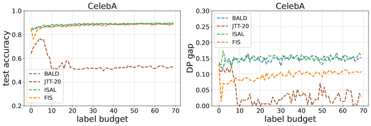
Figure 2: The impact of label budgets on the test accuracy & DP gap in the CelebA dataset. The binary classification targets is Smiling.

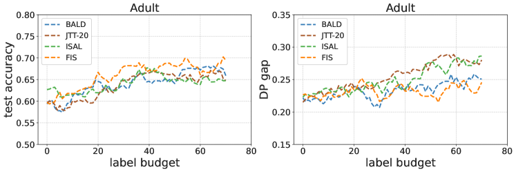
Figure 3: The impact of label budgets on the test accuracy & DP gap in the Adult dataset. The sensitive attribute is sex.

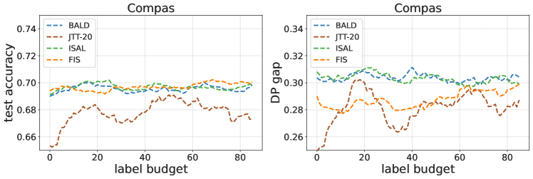
Figure 4: The impact of label budgets on the test accuracy & DP gap in the Compas dataset. The sensitive attribute is race.

Figure 5: We validate how accurate the first-order estimation of the influence is in comparison to the real influence. The $x$-axis represents the actual influence per sample, and the $y$-axis represents the estimated influence. We observe that while some of the examples are away from the diagonal line (which indicates the estimation is inaccurate), the estimated influence for most of the data samples are very close to their actual influence values.

References

- Siddiqi [2005] Naeem Siddiqi. Credit risk scorecards: Developing and implementing intelligent credit scoring. 2005.
- Carbonneau et al. [2008] Réal André Carbonneau, Kevin Laframboise, and Rustam M. Vahidov. Application of machine learning techniques for supply chain demand forecasting. Eur. J. Oper. Res., 184:1140–1154, 2008.
- Zicari et al. [2021] Roberto V. Zicari, James Brusseau, Stig Nikolaj Fasmer Blomberg, Helle Collatz Christensen, Megan Coffee, M. B. Ganapini, Sara Gerke, Thomas Krendl Gilbert, Eleanore Hickman, Elisabeth Hildt, Sune Holm, Ulrich Kühne, Vince Istvan Madai, Walter Osika, Andy Spezzatti, Eberhard Schnebel, Jesmin Jahan Tithi, Dennis Vetter, Magnus Westerlund, Reneé C. Wurth, Julia Amann, Vegard Antun, Valentina Beretta, Frédérick Bruneault, Erik Campano, Boris Düdder, Alessio Gallucci, Emmanuel Roberto Goffi, Christoffer Bjerre Haase, Thilo Hagendorff, Pedro Kringen, Florian Möslein, David J. Ottenheimer, Matiss Ozols, Laura Palazzani, Martin Petrin, Karin Tafur, Jim Tørresen, Holger Volland, and Georgios Kararigas. On assessing trustworthy ai in healthcare best practice for machine learning as a supportive tool to recognize cardiac arrest in emergency calls. 2021.
- Zhu et al. [2022] Zhaowei Zhu, Tianyi Luo, and Yang Liu. The rich get richer: Disparate impact of semi-supervised learning. In International Conference on Learning Representations, 2022. URL https://openreview.net/forum?id=DXPftn5kjQK.
- Donini et al. [2018] Michele Donini, Luca Oneto, Shai Ben-David, John S Shawe-Taylor, and Massimiliano Pontil. Empirical risk minimization under fairness constraints. Advances in neural information processing systems, 31, 2018.
- Hardt et al. [2016] Moritz Hardt, Eric Price, and Nati Srebro. Equality of opportunity in supervised learning. Advances in neural information processing systems, 29, 2016.
- Agarwal et al. [2018] Alekh Agarwal, Alina Beygelzimer, Miroslav Dudík, John Langford, and Hanna Wallach. A reductions approach to fair classification. In Proceedings of the 35th International Conference on Machine Learning (ICML ’18), 2018.
- Zafar et al. [2017] Muhammad Bilal Zafar, Isabel Valera, Manuel Gomez Rodriguez, and Krishna P Gummadi. Fairness constraints: Mechanisms for fair classification. In Proceedings of the 20th International Conference on Artificial Intelligence and Statistics (AISTATS), 2017.
- Wang et al. [2022a] Jialu Wang, Xin Eric Wang, and Yang Liu. Understanding instance-level impact of fairness constraints. In International Conference on Machine Learning, pages 23114–23130. PMLR, 2022a.
- Wei et al. [2023a] Jiaheng Wei, Zhaowei Zhu, Gang Niu, Tongliang Liu, Sijia Liu, Masashi Sugiyama, and Yang Liu. Fairness improves learning from noisily labeled long-tailed data. arXiv preprint arXiv:2303.12291, 2023a.
- Zhu et al. [2023] Zhaowei Zhu, Yuanshun Yao, Jiankai Sun, Hang Li, and Yang Liu. Weak proxies are sufficient and preferable for fairness with missing sensitive attributes. In International Conference on Machine Learning, pages 43258–43288. PMLR, 2023.
- Kleinberg et al. [2016] Jon Kleinberg, Sendhil Mullainathan, and Manish Raghavan. Inherent trade-offs in the fair determination of risk scores. arXiv preprint arXiv:1609.05807, 2016.
- Lewis and Catlett [1994] David D Lewis and Jason Catlett. Heterogeneous uncertainty sampling for supervised learning. In Machine learning proceedings 1994, pages 148–156. Elsevier, 1994.
- Lindenbaum et al. [2004] Michael Lindenbaum, Shaul Markovitch, and Dmitry Rusakov. Selective sampling for nearest neighbor classifiers. Machine learning, 54:125–152, 2004.
- Dasgupta and Hsu [2008] Sanjoy Dasgupta and Daniel Hsu. Hierarchical sampling for active learning. In Proceedings of the 25th international conference on Machine learning, pages 208–215, 2008.
- Wang et al. [2012] Ran Wang, Sam Kwong, and Degang Chen. Inconsistency-based active learning for support vector machines. Pattern Recognition, 45(10):3751–3767, 2012.
- Hoi et al. [2006] Steven CH Hoi, Rong Jin, and Michael R Lyu. Large-scale text categorization by batch mode active learning. In Proceedings of the 15th international conference on World Wide Web, pages 633–642, 2006.
- Roy and McCallum [2001] Nicholas Roy and Andrew McCallum. Toward optimal active learning through monte carlo estimation of error reduction. ICML, Williamstown, 2:441–448, 2001.
- Liu et al. [2021a] Zhuoming Liu, Hao Ding, Huaping Zhong, Weijia Li, Jifeng Dai, and Conghui He. Influence selection for active learning. In Proceedings of the IEEE/CVF International Conference on Computer Vision, pages 9274–9283, 2021a.
- Wang et al. [2022b] Tianyang Wang, Xingjian Li, Pengkun Yang, Guosheng Hu, Xiangrui Zeng, Siyu Huang, Cheng-Zhong Xu, and Min Xu. Boosting active learning via improving test performance. In Proceedings of the AAAI Conference on Artificial Intelligence, volume 36, pages 8566–8574, 2022b.
- Hammoudeh and Lowd [2022] Zayd Hammoudeh and Daniel Lowd. Training data influence analysis and estimation: A survey. arXiv preprint arXiv:2212.04612, 2022.
- Xie et al. [2023] Yichen Xie, Han Lu, Junchi Yan, Xiaokang Yang, Masayoshi Tomizuka, and Wei Zhan. Active finetuning: Exploiting annotation budget in the pretraining-finetuning paradigm. In Proceedings of the IEEE/CVF Conference on Computer Vision and Pattern Recognition, pages 23715–23724, 2023.
- Asudeh et al. [2019] Abolfazl Asudeh, Zhongjun Jin, and HV Jagadish. Assessing and remedying coverage for a given dataset. In 2019 IEEE 35th International Conference on Data Engineering (ICDE), pages 554–565. IEEE, 2019.
- Azzalini et al. [2021] Fabio Azzalini, Chiara Criscuolo, and Letizia Tanca. Fair-db: Functional dependencies to discover data bias. In EDBT/ICDT Workshops, 2021.
- Tae and Whang [2021] Ki Hyun Tae and Steven Euijong Whang. Slice tuner: A selective data acquisition framework for accurate and fair machine learning models. In Proceedings of the 2021 International Conference on Management of Data, pages 1771–1783, 2021.
- Sharma et al. [2020] Shubham Sharma, Yunfeng Zhang, Jesús M Ríos Aliaga, Djallel Bouneffouf, Vinod Muthusamy, and Kush R Varshney. Data augmentation for discrimination prevention and bias disambiguation. In Proceedings of the AAAI/ACM Conference on AI, Ethics, and Society, pages 358–364, 2020.
- Celis et al. [2020] L Elisa Celis, Vijay Keswani, and Nisheeth Vishnoi. Data preprocessing to mitigate bias: A maximum entropy based approach. In International conference on machine learning, pages 1349–1359. PMLR, 2020.
- Chawla et al. [2002] Nitesh V Chawla, Kevin W Bowyer, Lawrence O Hall, and W Philip Kegelmeyer. Smote: synthetic minority over-sampling technique. Journal of artificial intelligence research, 16:321–357, 2002.
- Zemel et al. [2013] Rich Zemel, Yu Wu, Kevin Swersky, Toni Pitassi, and Cynthia Dwork. Learning fair representations. In International conference on machine learning, pages 325–333. PMLR, 2013.
- Chen et al. [2018] Irene Chen, Fredrik D Johansson, and David Sontag. Why is my classifier discriminatory? Advances in neural information processing systems, 31, 2018.
- Kamiran and Calders [2012] Faisal Kamiran and Toon Calders. Data preprocessing techniques for classification without discrimination. Knowledge and Information Systems, 33(1):1–33, 2012.
- Jiang and Nachum [2020] Heinrich Jiang and Ofir Nachum. Identifying and correcting label bias in machine learning. In International Conference on Artificial Intelligence and Statistics, pages 702–712. PMLR, 2020.
- Diesendruck et al. [2020] Maurice Diesendruck, Ethan R Elenberg, Rajat Sen, Guy W Cole, Sanjay Shakkottai, and Sinead A Williamson. Importance weighted generative networks. In Machine Learning and Knowledge Discovery in Databases: European Conference, ECML PKDD 2019, Würzburg, Germany, September 16–20, 2019, Proceedings, Part II, pages 249–265. Springer, 2020.
- Choi et al. [2020] Kristy Choi, Aditya Grover, Trisha Singh, Rui Shu, and Stefano Ermon. Fair generative modeling via weak supervision. In International Conference on Machine Learning, pages 1887–1898. PMLR, 2020.
- Qraitem et al. [2023] Maan Qraitem, Kate Saenko, and Bryan A Plummer. Bias mimicking: A simple sampling approach for bias mitigation. In Proceedings of the IEEE/CVF Conference on Computer Vision and Pattern Recognition, pages 20311–20320, 2023.
- Li and Vasconcelos [2019] Yi Li and Nuno Vasconcelos. Repair: Removing representation bias by dataset resampling. In Proceedings of the IEEE/CVF conference on computer vision and pattern recognition, pages 9572–9581, 2019.
- Feldman [2015] Michael Feldman. Computational fairness: Preventing machine-learned discrimination. PhD thesis, 2015.
- Feldman et al. [2015] Michael Feldman, Sorelle A Friedler, John Moeller, Carlos Scheidegger, and Suresh Venkatasubramanian. Certifying and removing disparate impact. In proceedings of the 21th ACM SIGKDD international conference on knowledge discovery and data mining, pages 259–268, 2015.
- Woodworth et al. [2017] Blake Woodworth, Suriya Gunasekar, Mesrob I Ohannessian, and Nathan Srebro. Learning non-discriminatory predictors. In Conference on Learning Theory, pages 1920–1953. PMLR, 2017.
- Pleiss et al. [2017] Geoff Pleiss, Manish Raghavan, Felix Wu, Jon Kleinberg, and Kilian Q Weinberger. On fairness and calibration. In Advances in Neural Information Processing Systems, pages 5680–5689, 2017.
- Menon and Williamson [2018] Aditya Krishna Menon and Robert C Williamson. The cost of fairness in binary classification. In Conference on Fairness, accountability and transparency, pages 107–118. PMLR, 2018.
- Prost et al. [2019] Flavien Prost, Hai Qian, Qiuwen Chen, Ed H Chi, Jilin Chen, and Alex Beutel. Toward a better trade-off between performance and fairness with kernel-based distribution matching. arXiv preprint arXiv:1910.11779, 2019.
- Li and Liu [2022] Peizhao Li and Hongfu Liu. Achieving fairness at no utility cost via data reweighing with influence. In International Conference on Machine Learning, pages 12917–12930. PMLR, 2022.
- Anahideh et al. [2022] Hadis Anahideh, Abolfazl Asudeh, and Saravanan Thirumuruganathan. Fair active learning. Expert Systems with Applications, 199:116981, 2022.
- Singh et al. [2021] Harvineet Singh, Rina Singh, Vishwali Mhasawade, and Rumi Chunara. Fairness violations and mitigation under covariate shift. In Proceedings of the 2021 ACM Conference on Fairness, Accountability, and Transparency, pages 3–13, 2021.
- Roh et al. [2023] Yuji Roh, Kangwook Lee, Steven Euijong Whang, and Changho Suh. Improving fair training under correlation shifts. arXiv preprint arXiv:2302.02323, 2023.
- Giguere et al. [2022] Stephen Giguere, Blossom Metevier, Yuriy Brun, Bruno Castro da Silva, Philip S Thomas, and Scott Niekum. Fairness guarantees under demographic shift. In Proceedings of the 10th International Conference on Learning Representations (ICLR), 2022.
- Hashimoto et al. [2018] Tatsunori Hashimoto, Megha Srivastava, Hongseok Namkoong, and Percy Liang. Fairness without demographics in repeated loss minimization. In International Conference on Machine Learning, pages 1929–1938. PMLR, 2018.
- Kirichenko et al. [2022] Polina Kirichenko, Pavel Izmailov, and Andrew Gordon Wilson. Last layer re-training is sufficient for robustness to spurious correlations. arXiv preprint arXiv:2204.02937, 2022.
- Liu et al. [2021b] Evan Z Liu, Behzad Haghgoo, Annie S Chen, Aditi Raghunathan, Pang Wei Koh, Shiori Sagawa, Percy Liang, and Chelsea Finn. Just train twice: Improving group robustness without training group information. In International Conference on Machine Learning, pages 6781–6792. PMLR, 2021b.
- Lahoti et al. [2020] Preethi Lahoti, Alex Beutel, Jilin Chen, Kang Lee, Flavien Prost, Nithum Thain, Xuezhi Wang, and Ed Chi. Fairness without demographics through adversarially reweighted learning. Advances in neural information processing systems, 33:728–740, 2020.
- Veldanda et al. [2023] Akshaj Kumar Veldanda, Ivan Brugere, Sanghamitra Dutta, Alan Mishler, and Siddharth Garg. Hyper-parameter tuning for fair classification without sensitive attribute access. arXiv preprint arXiv:2302.01385, 2023.
- Sohoni et al. [2020] Nimit Sohoni, Jared Dunnmon, Geoffrey Angus, Albert Gu, and Christopher Ré. No subclass left behind: Fine-grained robustness in coarse-grained classification problems. Advances in Neural Information Processing Systems, 33:19339–19352, 2020.
- Wei et al. [2023b] Jiaheng Wei, Harikrishna Narasimhan, Ehsan Amid, Wen-Sheng Chu, Yang Liu, and Abhishek Kumar. Distributionally robust post-hoc classifiers under prior shifts. arXiv preprint arXiv:2309.08825, 2023b.
- Zafar et al. [2019] Muhammad Bilal Zafar, Isabel Valera, Manuel Gomez-Rodriguez, and Krishna P Gummadi. Fairness constraints: A flexible approach for fair classification. The Journal of Machine Learning Research, 20(1):2737–2778, 2019.
- Shui et al. [2022] Changjian Shui, Gezheng Xu, Qi Chen, Jiaqi Li, Charles X Ling, Tal Arbel, Boyu Wang, and Christian Gagné. On learning fairness and accuracy on multiple subgroups. Advances in Neural Information Processing Systems, 35:34121–34135, 2022.
- Li et al. [2019] Tian Li, Maziar Sanjabi, Ahmad Beirami, and Virginia Smith. Fair resource allocation in federated learning. In International Conference on Learning Representations, 2019.
- Balashankar et al. [2019] Ananth Balashankar, Alyssa Lees, Chris Welty, and Lakshminarayanan Subramanian. What is fair? exploring pareto-efficiency for fairness constrained classifiers. arXiv preprint arXiv:1910.14120, 2019.
- Martinez et al. [2019] Natalia Martinez, Martin Bertran, and Guillermo Sapiro. Fairness with minimal harm: A pareto-optimal approach for healthcare. arXiv preprint arXiv:1911.06935, 2019.
- Feldman [2020] Vitaly Feldman. Does learning require memorization? a short tale about a long tail. In Proceedings of the 52nd Annual ACM SIGACT Symposium on Theory of Computing, pages 954–959, 2020.
- Pruthi et al. [2020] Garima Pruthi, Frederick Liu, Satyen Kale, and Mukund Sundararajan. Estimating training data influence by tracing gradient descent. In Advances in Neural Information Processing Systems, volume 33, pages 19920–19930, 2020.
- Koh and Liang [2017] Pang Wei Koh and Percy Liang. Understanding black-box predictions via influence functions. In International conference on machine learning, pages 1885–1894. PMLR, 2017.
- Zhu et al. [2021] Zhaowei Zhu, Yiwen Song, and Yang Liu. Clusterability as an alternative to anchor points when learning with noisy labels. In Marina Meila and Tong Zhang, editors, Proceedings of the 38th International Conference on Machine Learning, volume 139 of Proceedings of Machine Learning Research, pages 12912–12923. PMLR, 18–24 Jul 2021. URL https://proceedings.mlr.press/v139/zhu21e.html.
- Zhu et al. [2024] Zhaowei Zhu, Jialu Wang, Hao Cheng, and Yang Liu. Unmasking and improving data credibility: A study with datasets for training harmless language models. In The Twelfth International Conference on Learning Representations, 2024. URL https://openreview.net/forum?id=6bcAD6g688.
- Cheng et al. [2020] Hao Cheng, Zhaowei Zhu, Xingyu Li, Yifei Gong, Xing Sun, and Yang Liu. Learning with instance-dependent label noise: A sample sieve approach. arXiv preprint arXiv:2010.02347, 2020.
- Wei et al. [2022] Jiaheng Wei, Zhaowei Zhu, Hao Cheng, Tongliang Liu, Gang Niu, and Yang Liu. Learning with noisy labels revisited: A study using real-world human annotations. In International Conference on Learning Representations, 2022. URL https://openreview.net/forum?id=TBWA6PLJZQm.
- Liu et al. [2015] Ziwei Liu, Ping Luo, Xiaogang Wang, and Xiaoou Tang. Deep learning face attributes in the wild. In Proceedings of the IEEE international conference on computer vision, pages 3730–3738, 2015.
- Asuncion and Newman [2007] Arthur Asuncion and David Newman. Uci machine learning repository, 2007.
- Angwin et al. [2016] Julia Angwin, Jeff Larson, Surya Mattu, and Lauren Kirchner. Machine bias. 2016.
- Branchaud-Charron et al. [2021] Frédéric Branchaud-Charron, Parmida Atighehchian, Pau Rodríguez, Grace Abuhamad, and Alexandre Lacoste. Can active learning preemptively mitigate fairness issues? arXiv preprint arXiv:2104.06879, 2021.