Stochastic Graph Heat Modelling
for Diffusion-based Connectivity Retrieval

Abstract

Heat diffusion describes the process by which heat flows from areas with higher temperatures to ones with lower temperatures. This concept was previously adapted to graph structures, whereby heat flows between nodes of a graph depending on the graph topology. Here, we combine the graph heat equation with the stochastic heat equation, which ultimately yields a model for multivariate time signals on a graph. We show theoretically how the model can be used to directly compute the diffusion-based connectivity structure from multivariate signals. Unlike other connectivity measures, our heat model-based approach is inherently multivariate and yields an absolute scaling factor, namely the graph thermal diffusivity, which captures the extent of heat-like graph propagation in the data. On two datasets, we show how the graph thermal diffusivity can be used to characterise Alzheimer’s disease. We find that the graph thermal diffusivity is lower for Alzheimer’s patients than healthy controls and correlates with dementia scores, suggesting structural impairment in patients in line with previous findings.
Clinical relevance— This study introduces a novel heat-based connectivity measure, which allows to characterise Alzheimer’s disease in terms of the graph thermal diffusivity.

I Introduction

Diffusion encompasses the general notion that connected areas with differing concentrations, for example chemical concentrations or heat densities, are aimed at equalling each other out over time [1]. While diffusion processes are complex on a microscopic level, their macroscopic description often reduces to partial differential equations, such as the heat equation. This equation can be extended with an additional noise term, which yields the stochastic heat equation [2]. The noise term can be used to model chaotic microscopic effects and acts as a driving force for the system. Examples of these microscopic effects include molecular interactions or, as is the case in this work, neuronal noise.

Both the heat equation and its stochastic extension are continuous in space. The heat equation can be naturally discretised by replacing the Laplacian operator with the negative graph Laplacian, yielding the graph heat equation [3]. Crucially, the graph Laplacian can not only be used to describe discrete Euclidean topologies, such as grids, but also highly irregular graph topologies. Previous work has employed the graph heat equation to model multivariate signals using hidden heat sources learnt from the data [4].

In the current work, we combine the stochastic heat equation with the graph heat equation to model brain processing as a heat diffusion process driven by neuronal noise. On the one hand, this approach is motivated by the idea that multivariate neurophysiological signals reside on irregular graphs, which are a consequence of the complex connectivity structure in the brain [5]. On the other hand, it is underpinned by the widespread occurrence of neuronal noise in the brain and its potential role in driving neurons [6]. Importantly, the additional stochastic term allows to use the signal values themselves as the heat sources, which has the principal advantage that they can be directly inferred from the data.

We use this model to develop a novel functional connectivity measure as a heat diffusion graph. To this end, we firstly solve the stochastic graph heat equation and adapt it to discrete signals with measurement noise. We then solve this equation for the graph Laplacian using suitable approximations. Unlike common connectivity measures such as correlation, mutual information or Granger causality, which are bivariate [7], our diffusion-based connectivity measure is inherently multivariate. It further preserves the scale of the connectivity, which can be retrieved, for instance, as the spectral norm of the connectivity matrix. We refer to this scale as the graph thermal diffusivity. Using two datasets, we show that the graph thermal diffusivity is lower in routine electroencephalography (EEG) recordings of Alzheimer’s disease (AD) patients than in healthy controls. We further show a correlation of 0.35 between Mini-Mental State Examination (MMSE) scores and the graph thermal diffusivity. Our findings suggest structural impairments in AD patients, in line with the literature [8].

II Theory

II-A Stochastic Graph Heat Equation

The heat equation is given by the following second-order differential equation:

$$\frac{\partial}{\partial t}x(s,t)=\Delta x(s,t),$$ (1)

where $x(s,t)$ is a function, or field, in space and time and $\Delta$ is the Laplace operator. To model stochastic effects, a noise term can be added to equation (1), yielding the stochastic heat equation:

$$\frac{\partial}{\partial t}x(s,t)=\Delta x(s,t)+\sigma\frac{\partial}{\partial t}W(s,t),$$ (2)

where $W(s,t)$ and $\sigma$ denote a Wiener process and its scale, respectively. We here extend equation (2) to spatially discretised fields, i.d., time-continuous multivariate signals $\mathbf{x}(t)$ with an underlying spatial structure, which can be algebraically represented by an adjacency matrix $\mathbf{A}$. To discretise equation (2), the continuous fields $x(s,t)$ and $W(s,t)$ are on the one hand replaced by the spatial signal $\mathbf{x}(t)$ and a vector of Wiener processes $\mathbf{W}(t)=\left(W_{1}(t),...,W_{N}(t)\right)^{\top}$, respectively. On the other hand, the Laplace operator $\Delta$ is replaced by the negative graph Laplacian $\mathbf{L}=\mathbf{D}-\mathbf{A}$ [4], where $\mathbf{D}\coloneqq\mathrm{diag}(\mathbf{A}\cdot\mathbf{1})$ is the degree matrix, yielding overall:

$$\frac{\partial}{\partial t}\mathbf{x}(t)=-\mathbf{L}\mathbf{x}(t)+\sigma\frac{\partial}{\partial t}\mathbf{W}(t).$$ (3)

II-B Solution of the Stochastic Graph Heat Equation

An exact solution for the stochastic graph heat equation (3) is given by:

$$\mathbf{x}(t) =e^{-t\mathbf{L}}\left(\mathbf{x}_{0}+\int_{t_{0}}^{t}e^{\tau\mathbf{L}}\sigma\frac{\partial}{\partial\tau}\mathbf{W}(\tau)d\tau\right),$$ (4)

with the initial condition $\mathbf{x}(t_{0})=\mathbf{x}_{0}$. The validity of this solution can be shown by inserting $\mathbf{x}(t)$ into equation (3):

$$\frac{\partial}{\partial t}\mathbf{x}(t)=- \mathbf{L}e^{-t\mathbf{L}}\left(\mathbf{x}_{0}+\int_{t_{0}}^{t}e^{\tau\mathbf{L}}\sigma\frac{\partial}{\partial\tau}\mathbf{W}(\tau)d\tau\right)$$

$$+e^{-t\mathbf{L}}e^{t\mathbf{L}}\sigma\frac{\partial}{\partial t}\mathbf{W}(t)$$

$$=- \mathbf{L}\mathbf{x}(t)+\sigma\frac{\partial}{\partial t}\mathbf{W}(t).$$ (5)

II-C Model Sampling and Measurement Noise

Equation (4) describes the continuous evolution of the signal in time at discrete spatial locations. To model an experimental recording, the signal can be sampled at equidistant time steps $\Delta t$ determined by the device sampling rate. Generally, the time step $\Delta t$ is sufficiently small, such that the signal evolution can be approximated as follows:

$$\mathbf{x}(t+\Delta t)= e^{-(t+\Delta t)\mathbf{L}}\left(\mathbf{x}_{0}+\int_{t_{0}}^{t+\Delta t}e^{\tau\mathbf{L}}\sigma\frac{\partial}{\partial\tau}\mathbf{W}(\tau)d\tau\right)$$

$$= e^{-\Delta t\mathbf{L}}\left(\mathbf{x}(t)+\int_{t}^{t+\Delta t}e^{(\tau-t)\mathbf{L}}\sigma\frac{\partial}{\partial\tau}\mathbf{W}(\tau)d\tau\right)$$

$$\approx e^{-\Delta t\mathbf{L}}\left(\mathbf{x}(t)+\int_{t}^{t+\Delta t}\sigma\frac{\partial}{\partial\tau}\mathbf{W}(\tau)d\tau\right)$$

$$= e^{-\Delta t\mathbf{L}}\left(\mathbf{x}(t)+\mathbf{e}\right),$$ (6)

where $\mathbf{e}\sim\mathcal{N}(\mathbf{0},\sigma\Delta t)$ is a noise vector resulting from the definition of the Wiener process.

The signal $\mathbf{x}(t)$ corresponds to the system-internal signal. The external signal $\mathbf{x}^{\prime}(t)$ includes measurement errors and is defined as:

$$\mathbf{x}^{\prime}(t)\coloneqq \mathbf{x}(t)+\mathbf{e}^{\prime}$$ (7)

$$\Rightarrow\mathbf{x}^{\prime}(t+\Delta t)= e^{-\Delta t\mathbf{L}}\left(\mathbf{x}(t)+\mathbf{e}\right)+\mathbf{e}^{\prime},$$ (8)

with $\mathbf{e}^{\prime}\sim\mathcal{N}(\mathbf{0},\sigma^{\prime})$. The measurement error encompasses any external noise measured at the sensor which is not propagated by the system’s graph connectivity. Incidentally, equation (8) can be used to simulate multivariate signal with an underlying spatial structure given by $\mathbf{L}$ [9].

The sampled spatial signals $\mathbf{x}^{\prime}(t_{0}+k\Delta t)$, $k=0,...,N_{c}-1$, can be concatenated to yield the full multivariate signal as a data matrix $\mathbf{X}^{\prime}\in\mathbb{R}^{N_{c}\times N_{t}}$:

$$\mathbf{X}^{\prime}=\begin{bmatrix}\mathbf{x}^{\prime}(t_{0}),\mathbf{x}^{\prime}(t_{0}+\Delta t),...,\mathbf{x}^{\prime}(t_{0}+(N_{t}-1)\Delta t)\end{bmatrix}.$$ (9)

We further define data matrices $\mathbf{X}_{0}$ and $\mathbf{X}_{1}$ with index 0 or 1 by either removing the last column or the first column of $\mathbf{X}$, respectively. With these, the vector equation (8) can be rewritten as a matrix equation:

$$\mathbf{X}_{1}^{\prime} =e^{-\Delta t\mathbf{L}}\left(\mathbf{X}_{0}+\mathbf{E}\right)+\mathbf{E}_{1}^{\prime}$$

$$=e^{-\Delta t\mathbf{L}}\left(\mathbf{X}_{0}^{\prime}-\mathbf{E}_{0}^{\prime}+\mathbf{E}\right)+\mathbf{E}_{1}^{\prime},$$ (10)

where the noise matrices $\mathbf{E}\sim\mathcal{N}(\mathbf{0}_{N_{c}\times N_{t}},\sigma\Delta t)$ and $\mathbf{E}^{\prime}\sim\mathcal{N}(\mathbf{0}_{N_{c}\times N_{t}},\sigma^{\prime})$ are sampled from a multivariate normal distribution.

III Methods

III-A Heat Diffusion Graph Retrieval

This section shows how an algebraic heat graph can be retrieved from a multivariate signal governed by heat-like graph dynamics described in section II-B. The principal goal is to retrieve the graph Laplacian $\mathbf{L}$ from equation (10). Note that generally only the recorded signal $\mathbf{X}^{\prime}$ is given. However, assumptions about $\sigma\Delta t$ and $\sigma^{\prime}$ as well as noise term averages allow to infer the graph structure and the scale of the heat processing.

To simplify our calculations, we begin by defining the following two matrices:

$$\mathbf{M}_{1} =\mathbf{X}_{1}^{\prime}-\mathbf{E}_{1}^{\prime}$$ (11)

$$\mathbf{M}_{0} =\mathbf{X}_{0}^{\prime}-\mathbf{E}_{0}^{\prime}+\mathbf{E}_{0}.$$ (12)

We then insert these two definitions into equation (10) and solve the equation for $\mathbf{L}$, yielding:

$$\mathbf{M}_{1} =e^{-\Delta t\mathbf{L}}\mathbf{M}_{0}$$ (13)

$$\Leftrightarrow \mathbf{M}_{1}\mathbf{M}_{0}^{\top}(\mathbf{M}_{0}\mathbf{M}_{0}^{\top})^{-1} =e^{-\Delta t\mathbf{L}}$$ (14)

$$\Leftrightarrow \mathbf{L}=-\frac{1}{\Delta t}\log \left((\mathbf{M}_{1}\mathbf{M}_{0}^{\top})(\mathbf{M}_{0}\mathbf{M}_{0}^{\top})^{-1}\right).$$ (15)

We further make use of the fact that a noise matrix multiplied with any matrix other than itself averages to zero, and that for small enough time steps $\mathbf{X}_{1}^{\prime}$ contains the noise matrix $\mathbf{E}_{0}$. This yields the following approximations:

$$\mathbf{M}_{1}\mathbf{M}_{0}^{\top} \approx\mathbf{X}_{1}^{\prime}\mathbf{X}_{0}^{\prime\top}+\mathbf{X}_{1}^{\prime}\mathbf{E}_{0}^{\top}$$

$$\approx\mathbf{X}_{1}^{\prime}\mathbf{X}_{0}^{\prime\top}+\mathbf{E}_{0}\mathbf{E}_{0}^{\top}$$ (16)

$$\mathbf{M}_{0}\mathbf{M}_{0}^{\top} \approx\mathbf{X}_{0}^{\prime}\mathbf{X}_{0}^{\prime\top}+\mathbf{E}_{0}^{\prime}\mathbf{E}_{0}^{\prime\top}+\mathbf{E}_{0}\mathbf{E}_{0}^{\top}.$$ (17)

To estimate the remaining noise terms, we observe that for small $\Delta t$ equation (10) reduces to $\mathbf{X}_{1}^{\prime}-\mathbf{E}_{1}^{\prime}\approx\mathbf{X}_{0}^{\prime}-\mathbf{E}_{0}^{\prime}+\mathbf{E}_{0}$, such that:

$$\left(\mathbf{X}_{1}^{\prime}-\mathbf{X}_{0}^{\prime}\right)\left(\mathbf{X}_{1}^{\prime}-\mathbf{X}_{0}^{\prime}\right)^{\top}\approx\mathbf{E}_{0}^{\prime}\mathbf{E}_{0}^{\prime\top}+\mathbf{E}_{0}\mathbf{E}_{0}^{\top}+\mathbf{E}_{1}^{\prime}\mathbf{E}_{1}^{\prime\top}.$$ (18)

Without prior knowledge about the standard deviations $\sigma\Delta t$ and $\sigma^{\prime}$, we may assume $\sigma\Delta t\approx\sigma^{\prime}$, allowing us to estimate:

$$\mathbf{E}_{0}^{\prime}\mathbf{E}_{0}^{\prime\top} \approx\mathbf{E}_{0}\mathbf{E}_{0}^{\top}\approx\mathbf{E}_{1}^{\prime}\mathbf{E}_{1}^{\prime\top}$$

$$\approx\frac{1}{3}\left(\mathbf{X}_{1}^{\prime}-\mathbf{X}_{0}^{\prime}\right)\left(\mathbf{X}_{1}^{\prime}-\mathbf{X}_{0}^{\prime}\right)^{\top}\eqqcolon\tilde{\mathbf{E}}\tilde{\mathbf{E}}^{\top}.$$ (19)

Inserting these approximations into equations (16) and (17) yields:

$$\mathbf{M}_{1}\mathbf{M}_{0}^{\top} \approx\mathbf{X}_{1}^{\prime}\mathbf{X}_{0}^{\prime\top}+\tilde{\mathbf{E}}\tilde{\mathbf{E}}^{\top}$$ (20)

$$\mathbf{M}_{0}\mathbf{M}_{0}^{\top} \approx\mathbf{X}_{0}^{\prime}\mathbf{X}_{0}^{\prime\top}+2\tilde{\mathbf{E}}\tilde{\mathbf{E}}^{\top}.$$ (21)

These approximations can finally be inserted into equation (15), such that the graph Laplacian $\mathbf{L}$ is given solely in terms of the recorded data matrix $\mathbf{X}^{\prime}$ and the sampling resolution $\Delta t$:

$$\mathbf{L}\approx-\frac{1}{\Delta t}\log\biggl{(} \Bigl{(}\mathbf{X}_{1}^{\prime}\mathbf{X}_{0}^{\prime\top}+\frac{1}{3}\left(\mathbf{X}_{1}^{\prime}-\mathbf{X}_{0}^{\prime}\right)\left(\mathbf{X}_{1}^{\prime}-\mathbf{X}_{0}^{\prime}\right)^{\top}\Bigr{)}$$

$$\Bigl{(}\mathbf{X}_{0}^{\prime}\mathbf{X}_{0}^{\prime\top}+\frac{2}{3}(\mathbf{X}_{1}^{\prime}-\mathbf{X}_{0}^{\prime})(\mathbf{X}_{1}^{\prime}-\mathbf{X}_{0}^{\prime})^{\top}\Bigr{)}^{-1}\biggr{)}.$$ (22)

III-B Graph Laplacian Constraints

In general, the graph Laplacian computed in equation (22) does not yet satisfy all the properties of a Laplacian corresponding to an undirected, non-negative graph $\mathbf{A}$, which are:

$$(i)\phantom{ii} \mathrm{diag}(\mathbf{L}) =\mathbf{A}\cdot\mathbf{1},$$ (23)

$$(ii)\phantom{i} \mathbf{A} =\mathbf{A}^{\top},$$ (24)

$$(iii) [\mathbf{A}]_{ij} \geq 0.$$ (25)

By imposing these constraints on $\mathbf{L}$, we can further improve the retrieval of the graph Laplacian $\mathbf{L}$ in equation (22) . To enforce properties (ii) and (iii), we simply symmetrise the adjacency matrix and set all negative elements to zero:

$$\mathbf{A}_{s} =\frac{\mathbf{A}+\mathbf{A}^{\top}}{2},$$ (26)

$$[\mathbf{A}_{s+}]_{ij} =\max([\mathbf{A}_{s}]_{ij},0).$$ (27)

To enforce constraint (i), we firstly compute the degree matrix $\mathbf{D}_{s+}=\mathrm{diag}(\mathbf{A}_{s+}\cdot\mathbf{1})$. To include the information given in the measured degree matrix $\mathbf{D}=\mathbf{L}-\mathbf{A}$, we mix $\mathbf{D}_{s+}$ with $\mathbf{D}$ to yield the diagonal degree matrix $\tilde{\mathbf{D}}$:

$$[\tilde{\mathbf{D}}]_{ii}=\sqrt{\frac{\max([\mathbf{D}]_{ii},0)+[\mathbf{D}_{s+}]_{ii}}{2[\mathbf{D}_{s+}]_{ii}}},$$ (28)

Note that we limited $[\mathbf{D}]_{ii}$ to non-negative values to ensure that the argument of the root is positive. Finally, the adjacency matrix satisfying all three properties is given by:

$$\tilde{\mathbf{A}}=\tilde{\mathbf{D}}^{1/2}\mathbf{A}_{s+}\tilde{\mathbf{D}}^{1/2},$$ (29)

from which the final graph Laplacian can be inferred as $\tilde{\mathbf{L}}=\mathrm{diag}(\tilde{\mathbf{A}}\cdot\mathbf{1})-\tilde{\mathbf{A}}$.

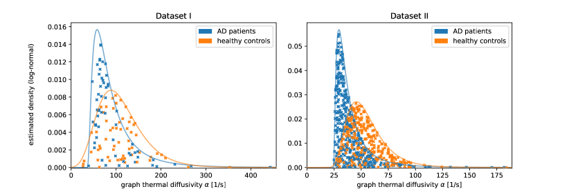
Figure 1: Graph thermal diffusivity distributions for dataset I (left) and dataset II (right) for AD patients (blue) and healthy controls (orange) using a propagation time of $\Delta t\approx 30\,\mathrm{ms}$. The distributions were modelled as log-normal distributions due to the boundedness of the diffusivity. Notably, the distributions for the AD patients are shifted towards lower diffusivity values for both datasets, which indicates that brain activity does not spread, or diffuse, as effectively for AD patients as compared to healthy controls. The location of the distributions for each condition are different between the two datasets, which may be due to differences in the EEG setup and montage as well as differences in the signal preprocessing

III-C Graph Thermal Diffusivity

Our proposed method estimates a graph structure in the multivariate signal scaled in terms of its dynamic evolution. To explicitly retrieve this scale, we normalise the final Laplacian matrix by its spectral norm $\lVert\tilde{\mathbf{L}}\rVert_{2}=\lambda_{max}(\tilde{\mathbf{L}})$, such that $\alpha\coloneqq\lambda_{max}(\tilde{\mathbf{L}})$ is the scale of heat-like processing in the data matrix, given in units of $1/\mathrm{s}$. In analogy with the classical heat model, we term $\alpha$ the graph thermal diffusivity.

IV Experiments

IV-A Dataset I

The first routine EEG dataset used in this study was recorded on 20 Alzheimer’s patients and 20 healthy controls at a sampling rate of $2048\,\mathrm{Hz}$. Participants were instructed to close their eyes during the recording. A combination of the 10-20 and the 10-10 electrode placement system was used, from which 23 bipolar channels were created. For each patient, two or three samples with a length of 12 seconds were selected from the recording, resulting in overall 119 samples. More details about the dataset can be found in [10].

IV-B Dataset II

The second dataset is publicly available and was recorded on 36 Alzheimer’s disease patients and 29 healthy controls [11]. It was acquired using an EEG system with 19 scalp electrodes placed according to the 10-20 system and two reference electrodes, sampled at a rate of 500 Hz. In addition, MMSE scores were taken for each participant. Similar to dataset I, participants were directed to close their eyes throughout the recordings, which lasted for approximately 13-14 minutes on average. Additional information regarding the dataset and preprocessing steps can be found in Miltiadous et al. [11]. We partitioned the preprocessed EEG samples into segments lasting 60 seconds each, with the exclusion of samples containing artifacts. This partitioning resulted in a total of 656 EEG samples.

IV-C Experimental Setup

In our experiment, we computed the graph thermal diffusivity $\alpha$ in the filtered EEG samples for the two datasets using a propagation time of $\Delta t\approx 30\,\mathrm{ms}$. To filter the data, we applied a Butterworth bandpass filter between 0.5 $\mathrm{Hz}$ and 45 $\mathrm{Hz}$. The time step is set by downsampling datasets I and II by factors of 61 and 15, respectively. This time step is informed by typical brain signal propagation speeds, which are on the order of $v=1\,\mathrm{m}/\mathrm{s}$. For example, Halgren et al. measured the alpha rhythm propagation in human cortex as $v=0.91\,\mathrm{m}/\mathrm{s}$ [12], which would correspond to a propagation distance of $\Delta x\approx 30\,\mathrm{mm}$ with $\Delta t\approx 30\,\mathrm{ms}$.

IV-D Results

Figure 1 shows the retrieved diffusivity $\alpha$ values for AD patients in blue and healthy controls in orange. We fitted log-normal distributions, suitable due to their boundedness at zero and good fit, to the results using the Python distfit package [13]. Most notably, the distributions of the graph thermal diffusivity are consistently shifted towards lower values for AD patients. We also compute the Pearson correlation coefficient between the MMSE score and the graph thermal connectivity for dataset II as $0.35$.

V Discussion

In this study, we have introduced a novel connectivity measure based on heat diffusion-like signal propagation. The connectivity measure is inherently multivariate and yields a scaling factor, the so-called graph thermal diffusivity. In our EEG-based experiments, we have observed a shift in towards lower diffusivity values in AD patients, which indicates that the brain processing may be more local. We therefore interpret the increase of low diffusivity values in AD patients as a consequence of structural impairment in those patients [8]. In addition, we have found a significant correlation between the MMSE score and the graph thermal diffusivity, giving further evidence for the link between AD and the graph thermal connectivity. We believe that the diffusivity may contribute to EEG-based AD diagnosis as an additional classification feature.

Our method has several limitations. Firstly, it involves several approximations, which may not be valid in every setting. Secondly, our method requires the computation of a matrix inverse, which may lead to unreliable results if the matrix is ill-conditioned. Lastly, the simplicity of the underlying model may not adequately capture the complexity of EEG data and is limited to only one time scale. Despite these challenges, our experimental AD characterisation results showcase the value of the heat diffusion connectivity measure and its scaling factor, the graph thermal diffusivity. Due to the simplicity of the model, we hypothesise that our method may be applicable to a broader range of problems involving multivariate signals.

References

- [1] J. Crank, The mathematics of diffusion. Oxford university press, 1979.
- [2] I. Corwin and H. Shen, “Some recent progress in singular stochastic partial differential equations,” Bulletin of the American Mathematical Society, vol. 57, no. 3, pp. 409–454, 2020.
- [3] B. Xiao, E. R. Hancock, and R. C. Wilson, “Graph characteristics from the heat kernel trace,” Pattern Recognition, vol. 42, no. 11, pp. 2589–2606, 2009.
- [4] D. Thanou, X. Dong, D. Kressner, and P. Frossard, “Learning heat diffusion graphs,” IEEE Transactions on Signal and Information Processing over Networks, vol. 3, no. 3, pp. 484–499, 2017.
- [5] S. Atasoy, I. Donnelly, and J. Pearson, “Human brain networks function in connectome-specific harmonic waves,” Nature communications, vol. 7, no. 1, p. 10340, 2016.
- [6] D. Guo, M. Perc, T. Liu, and D. Yao, “Functional importance of noise in neuronal information processing,” Europhysics Letters, vol. 124, no. 5, p. 50001, 2018.
- [7] A. M. Bastos and J.-M. Schoffelen, “A tutorial review of functional connectivity analysis methods and their interpretational pitfalls,” Frontiers in systems neuroscience, vol. 9, p. 175, 2016.
- [8] Z. Dai and Y. He, “Disrupted structural and functional brain connectomes in mild cognitive impairment and alzheimer’s disease,” Neuroscience Bulletin, vol. 30, pp. 217–232, 2014.
- [9] S. Goerttler, M. Wu, and F. He, “The effect of graph frequencies on dynamic structures in graph signal processing,” in 2022 IEEE Signal Processing in Medicine and Biology Symposium (SPMB). IEEE, 2022, pp. 1–6.
- [10] D. J. Blackburn, Y. Zhao, M. De Marco, S. M. Bell, F. He, H.-L. Wei, S. Lawrence, Z. C. Unwin, M. Blyth, J. Angel et al., “A pilot study investigating a novel non-linear measure of eyes open versus eyes closed eeg synchronization in people with alzheimer’s disease and healthy controls,” Brain sciences, vol. 8, no. 7, p. 134, 2018.
- [11] A. Miltiadous, K. D. Tzimourta, T. Afrantou, P. Ioannidis, N. Grigoriadis, D. G. Tsalikakis, P. Angelidis, M. G. Tsipouras, E. Glavas, N. Giannakeas et al., “A dataset of eeg recordings from: Alzheimer’s disease, frontotemporal dementia and healthy subjects,” OpenNeuro.[Dataset], 2023.
- [12] M. Halgren, I. Ulbert, H. Bastuji, D. Fabó, L. Erőss, M. Rey, O. Devinsky, W. K. Doyle, R. Mak-McCully, E. Halgren et al., “The generation and propagation of the human alpha rhythm,” Proceedings of the National Academy of Sciences, vol. 116, no. 47, pp. 23 772–23 782, 2019.
- [13] E. Taskesen, “distfit is a python library for probability density fitting.” Jan. 2020. [Online]. Available: https://erdogant.github.io/distfit