When and How: Learning Identifiable Latent States for
Nonstationary Time Series Forecasting

When and How: Learning Identifiable Latent States for
Nonstationary Time Series Forecasting

Abstract

Temporal distribution shifts are ubiquitous in time series data. One of the most popular methods assumes that the temporal distribution shift occurs uniformly to disentangle the stationary and nonstationary dependencies. But this assumption is difficult to meet, as we do not know when the distribution shifts occur. To solve this problem, we propose to learn IDentifiable latEnt stAtes (IDEA) to detect when the distribution shifts occur. Beyond that, we further disentangle the stationary and nonstationary latent states via sufficient observation assumption to learn how the latent states change. Specifically, we formalize the causal process with environment-irrelated stationary and environment-related nonstationary variables. Under mild conditions, we show that latent environments and stationary/nonstationary variables are identifiable. Based on these theories, we devise the IDEA model, which incorporates an autoregressive hidden Markov model to estimate latent environments and modular prior networks to identify latent states. The IDEA model outperforms several latest nonstationary forecasting methods on various benchmark datasets, highlighting its advantages in real-world scenarios.

1 Introduction

Time series forecasting (Zhou et al., 2021; Lim & Zohren, 2021; Rangapuram et al., 2018; Chatfield, 2000; Zhang, 2003) is known as one of the fundamental problems in machine learning and has achieved pioneering applications in various fields (Bi et al., 2023; Wu et al., 2023; Sezer et al., 2020). However, the inherent non-stationarity of time series data hinders the forecasting models from generalizing on the temporally varying distribution shift.

Several methodologies are proposed to solve this problem, which can be categorized into two types according to the inter-instance and intra-instance temporal distribution shift assumptions. The first type of method assumes that the shift occurs among instances, and each sequence instance is stationary (Li et al., 2023b; Oreshkin et al., 2021). Therefore, instance normalization (Kim et al., 2021) or nonstationary attention mechanism (Liu et al., 2022) are used to remove nonstationary components and compensate for them in prediction. Another type assumes that the environment changes uniformly (Liu et al., 2023c; Surana, 2020). Therefore, some researchers adopt stationarization (Virili & Freisleben, 2000) to remove nonstationarity from time series data. And (Liu et al., 2022) partitions the time-series data into equally-sized and stationary segments and uses the Fast Fourier Transform to select stationary and nonstationary components. In summary, these methods aim to disentangle the stationary and nonstationary dependency. More discussion about related works can be found in Appendix A.

Although current methods mitigate the temporal distribution shift to some extent, the assumptions they require are too strict since each sequence instance or segment may not be stationary when the environment labels are unknown. Figure 1 illustrates toy examples where a nonstationary sine curve is influenced by the nonstationary latent variable (amplitude) and stationary latent variables (frequency and phase). As shown in Figure 1 (a), existing methods split the nonstationary time series into three equal-size subsequences, but the purple and green curves are still nonstationary, making it difficult to disentangle the stationary and nonstationary latent variables. Furthermore, according to Figure 1 (b), even when latent environments are estimated correctly, if the latent variables are entangled, that is, the estimated amplitude and phase are not identified to change simultaneously, the forecasting model can still achieve suboptimal results.

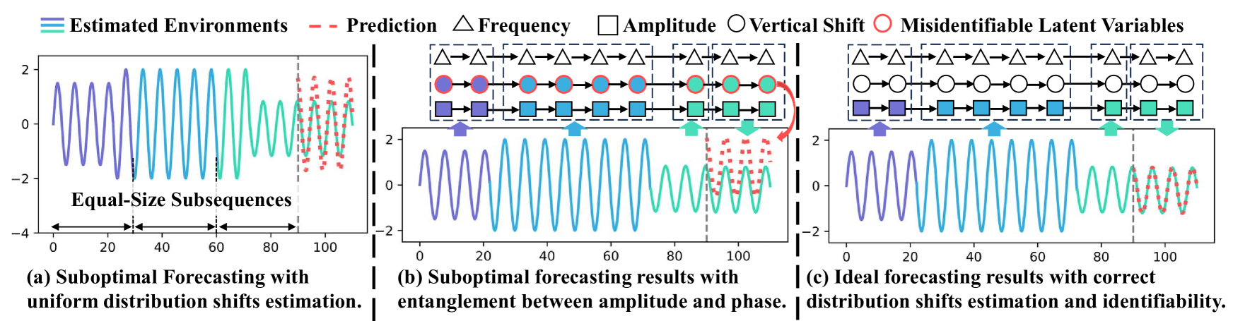
Figure 1: Illustration of nonstationary time series generated from nonstationary amplitude $\square$ (colored graphics) as well as stationary frequency $\triangle$ and vertical shift $\bigcirc$ (white graphics). (a) Methods with a uniform temporal distribution shift assumption cannot disentangle variant and invariant dependencies from the nonstationary segment (green curve), so the prediction with an average amplitude is generated. (b) Even when the latent environments are estimated correctly, the estimated amplitude and vertical shift are entangled, and the vertical shift is considered to change across environments mistakenly, so the upward bias predictions are obtained. (c)With correct environment estimation and latent variable disentanglement, we can achieve ideal forecasting performance. (Best view in color.)

Based on the above examples, an intuitive solution to nonstationary time series forecasting is shown in Figure 1 (c), showing that we should first detect when the temporal distribution shift occurs and then disentangle the stationary/nonstationary states to learn how they change across time. Under this intuition, we find that the latent environments and the stationary/nonstationary variables can be identified theoretically via sufficient observation assumption of nonstationarity. Therefore, we first consider a data generation process for nonstationary time series data. Sequentially, we employ sufficient observations assumption to present an identification theory for latent environments. We further prove that the stationary and nonstationary latent variables are identifiable. Following the theoretical results, we devise a model named IDEA to learn identifiable latent states for nonstationary time series forecasting. Specifically, the proposed IDEA is built on a variational inference framework, incorporating an autoregressive hidden Markov model to estimate latent environments and modular prior network architectures to identify stationary and nonstationary latent variables. Evaluation of simulation and eight real-world benchmark datasets demonstrate the accuracy of latent environment estimation and identification of latent states, as well as the effectiveness of real-world applications.

2 Identifying Distribution of Time Series Data

2.1 Data Generation Process for Time Series Data

To illustrate how we address the nonstationary time series forecasting problem, we begin with the data generation process as shown in Figure 2. Suppose that we have time series data with discrete time steps, ${\mathbf{x}}=\{{\mathbf{x}}_{1},{\mathbf{x}}_{2},\cdots,{\mathbf{x}}_{T}\}$, where ${\mathbf{x}}_{t}\in\mathbb{R}$ are generated from latent variables ${\mathbf{z}}_{t}\in\mathcal{Z}\subseteq\mathbb{R}^{n}$ by an invertible and non-linear mixing function $g$.

$$\vspace{-2.5mm}\small{\mathbf{x}}_{t}=g({\mathbf{z}}_{t}).$$ (1)

Note that ${\mathbf{z}}_{t}$ are divided into two parts, i.e., ${\mathbf{z}}_{t}=\{{\mathbf{z}}^{s}_{t},{\mathbf{z}}^{e}_{t}\}$, where ${\mathbf{z}}^{s}_{t}\in\mathbb{R}^{n_{s}}$ denote the environment-irrelated stationary latent variables, ${\mathbf{z}}^{e}_{t}\in\mathbb{R}^{n_{e}}$ denote the environment-related nonstationary latent variables, and $n_{e}+n_{s}=n$. Specifically, the $i$-th dimension stationary latent variable ${\mathbf{z}}_{t,i}^{s}$ are time-delayed and causally related to the historical stationary latent variables ${\mathbf{z}}_{t-\tau}^{s}$ with the time lag of $\tau$ via a nonparametric function $f_{i}^{s}$, which is formalized as follows:

$$\small z_{t,i}^{s}\!=\!f^{s}_{i}(\{z^{s}_{t-\tau,k}|z^{s}_{t-\tau,k}\!\in\!\mathbf{Pa}(z_{t,i}^{s})\},\epsilon^{s}_{t,i})\ \ \text{with}\ \ \epsilon^{s}_{t,i}\sim p_{\epsilon_{i}^{s}},$$ (2)

where $\mathbf{Pa}(z_{t,i}^{s})$ denotes the set of latent variables that directly cause ${\mathbf{z}}^{s}_{t,i}$ and $\epsilon^{s}_{t,i}$ denotes the temporally and spatially independent noise extracted from a distribution $p_{\epsilon_{i}^{s}}$. Moreover, the nonstationary latent variables ${\mathbf{z}}^{e}_{t}$ are influenced by the latent and discrete environment variables ${\mathbf{e}}_{t}$, which follows a first-order Markov process with $\bm{\mathrm{E}}\times\bm{\mathrm{E}}$ transition matrix $\bm{\mathrm{A}}$ and $\bm{\mathrm{E}}$ is the cardinality of ${\mathbf{e}}_{t}$. More specifically, we let the $(k,l)$-th entry $\bm{\mathrm{A}}_{k,l}$ be the probability from the state $k$ to the state $l$. As a result, the generation process of the $j$-th dimension nonstationary latent variable ${\mathbf{z}}_{t,j}^{e}$ can be formalized as follows:

$$\vspace{-1.5mm}\small\left\{\begin{array}[]{l}{\mathbf{e}}_{1},{\mathbf{e}}_{2},\cdots,{\mathbf{e}}_{T}\sim\text{Markov Chain}(\mathbf{A})\\ z_{t,j}^{e}=f^{e}_{j}({\mathbf{e}}_{t},\epsilon^{e}_{t,j})\ \ \text{with}\ \ \epsilon^{e}_{t,j}\sim p_{\epsilon_{j}^{e}},\end{array}\right.\vspace{0.5mm}$$ (3)

in which $f_{j}^{e}$ is a bijection function and $\epsilon^{e}_{t,j}$ is the mutually-independent noise extracted from $p_{\epsilon_{j}^{e}}$.

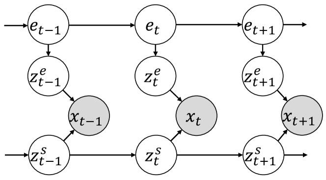
Figure 2: Data generation process of nonstationary time series. ${\mathbf{e}}_{t}$ denote the discrete latent environment variables, ${\mathbf{z}}_{t}^{e}$ denote the nonstationary latent variables, and ${\mathbf{z}}_{t}^{s}$ denote the stationary latent variables. We assume that the number of ${\mathbf{e}}$ is known, but when the temporal distribution shift occurs is unknown.

To better understand the data generation process as shown in Figure 2, we provide an easily comprehensible example of human driving. First, we let ${\mathbf{x}}_{t}$ be the speed of a car. Then ${\mathbf{e}}_{t}$ denotes the action of the driver, i.e., speeding or braking, and ${\mathbf{z}}^{e}_{t}$ denotes the engine power or acceleration. Finally, ${\mathbf{z}}_{t}^{s}$ denotes road conditions such as flat and slippery roads, which are irrelated to the actions.

2.2 Identifying Distribution of Time Series Data for Nonstationary Time Series Forecasting

Based on the aforementioned data generation process, we aim to address the nonstationary time series forecasting problem, i.e., to predict the future observation $\{{\mathbf{x}}_{t+1},{\mathbf{x}}_{t+2},\cdots,{\mathbf{x}}_{T}\}$ only from the historical observation data $\{{\mathbf{x}}_{1},{\mathbf{x}}_{2},\cdots,{\mathbf{x}}_{t}\}$. Mathematically, our goal is to identify the joint distribution of the historical and future time series data. By combining the generation mechanism of Fig. 2, the joint distribution can be further derivated as follows:

$$\vspace{-2mm}\small\begin{split}p({\mathbf{x}})=&\sum_{{\mathbf{e}}}\int_{{\mathbf{z}}^{e}}\int_{{\mathbf{z}}^{s}}p({\mathbf{x}},{\mathbf{e}},{\mathbf{z}}^{e},{\mathbf{z}}^{s})d_{{\mathbf{z}}^{e}}d_{{\mathbf{z}}^{s}}\\ =&\sum_{{\mathbf{e}}}\int_{{\mathbf{z}}^{e}}\int_{{\mathbf{z}}^{s}}p({\mathbf{x}}|{\mathbf{z}}^{e},{\mathbf{z}}^{s})p({\mathbf{z}}^{e}|{\mathbf{e}})p({\mathbf{e}})p({\mathbf{z}}^{s})d_{{\mathbf{z}}^{e}}d_{{\mathbf{z}}^{s}},\end{split}$$ (4)

where ${\mathbf{e}}:=\{{\mathbf{e}}_{1},\cdots,{\mathbf{e}}_{T}\},{\mathbf{z}}^{e}:=\{{\mathbf{z}}^{e}_{1},\cdots,{\mathbf{z}}^{e}_{T}\}$, and ${\mathbf{z}}^{s}:=\{{\mathbf{z}}^{s}_{1},\cdots,{\mathbf{z}}^{s}_{T}\}$ (we omit the subscripts due to limited space). Therefore, the joint distribution is identifiable by modeling the following four distributions: 1) the generative model of observations given stationary and nonstationary latent variables, i.e., $p({\mathbf{x}}|{\mathbf{z}}^{e},{\mathbf{z}}^{s})$; 2) the marginal distribution of latent environment variables, i.e. $p({\mathbf{e}})$ (Theorem 3.1); 3) the distribution of stationary latent variables,i.e., $p({\mathbf{z}}^{s})$ (Theorem 3.2); and 4) the conditional distribution of nonstationary latent variables, i.e., $p({\mathbf{z}}^{e}|{\mathbf{e}})$ (Theorem 3.3).

3 Identification of Latent Variables Under Sufficient Observation

In this section, we show the identifiability of these latent variables. To well establish the identification results of latent variables, we first illustrate the intuition behind the theories. Without any further assumptions, ${\mathbf{z}}_{t}^{s}$ and ${\mathbf{z}}_{t}^{e}$ are symmetric with ${\mathbf{x}}_{t}$, implying the simultaneous changing of ${\mathbf{z}}_{t}^{s}$ and ${\mathbf{z}}_{t}^{e}$, which makes it hard to disentangle ${\mathbf{z}}_{t}^{s}$ and ${\mathbf{z}}_{t}^{e}$ since ${\mathbf{z}}_{t}^{e}$ is mutually dependent without given ${\mathbf{e}}_{t}$. To break this restriction, we propose the Sufficient Observations assumption, which requires at least 2 consecutive observations for each environment. Therefore, for any three consecutive observations ${\mathbf{x}}_{1},{\mathbf{x}}_{2},{\mathbf{x}}_{3}$, the case where their corresponding environments are different, that is, ${\mathbf{e}}_{1}\neq{\mathbf{e}}_{2}\neq{\mathbf{e}}_{3}$, can be excluded. As a result, we can disentangle ${\mathbf{z}}_{t}^{s}$ and ${\mathbf{z}}_{t}^{e}$. In the following, we first show how to identify latent environments with Theorem 3.1, which addresses when the temporal distribution shift occurs. Then we show how to disentangle the stationary and nonstationary latent variables, i.e., ${\mathbf{z}}_{t}^{s}$ and ${\mathbf{z}}_{t}^{e}$, with Theorem 3.2 and 3.3, which addresses how the stationary and nonstationary latent variables change over time. Please refer to Appendix B for more details on the definition of identification up to label swapping and component-wise identification as well as the subspace identification.

3.1 Identification of Latent Environment Variables ${\mathbf{e}}_{t}$

To identify when the temporal distribution shift occurs and estimate the marginal distribution $p({\mathbf{e}})$, we propose the identification theory of latent environment variables ${\mathbf{e}}_{t}$, which is shown as Theorem 3.1.

Theorem 3.1.

(Identification of the latent environment ${\mathbf{e}}_{t}$.) Suppose the observed data is generated following the data generation process in Figure 2 and Equation (1)-(3). Then we further make the following assumptions:

• A3.1.1 (Prior Environment Number:) The number of latent environments of the Markov process, $\bm{\mathrm{E}}$, is known.

• A3.1.2 (Full Rank:) The transition matrix $\mathbf{A}$ is full rank.

• A3.1.3 (Linear Independence:) For ${\mathbf{e}}_{t}=1,2,\cdots,E$, the probability measures $\mu_{e}=p({\mathbf{x}}_{t}|{\mathbf{z}}_{t}^{e},{\mathbf{e}}_{t})$ are linearly independence and for any two different probability measures $\mu_{i},\mu_{j}$, their ratio $\frac{\mu_{i}}{\mu_{j}}$ are linearly independence.

• A3.1.4 (Sufficient Observation:) For each ${\mathbf{e}}_{t}=\{1,\!\cdots,\!\bm{\mathrm{E}}\}$, there are at least 2 consecutive observations.

Then, by modeling the observations ${\mathbf{x}}_{1},{\mathbf{x}}_{2},\cdots,{\mathbf{x}}_{t}$, the joint distribution of the corresponding latent environment variables $p({\mathbf{e}}_{1},{\mathbf{e}}_{2},\cdots,{\mathbf{e}}_{t})$ is identifiable up to label swapping of the hidden environment.

Proof Sketch. First, given any three consecutive observations ${\mathbf{x}}_{1},{\mathbf{x}}_{2},{\mathbf{x}}_{3}$ with the corresponding latent environments ${\mathbf{e}}_{1},{\mathbf{e}}_{2},{\mathbf{e}}_{3}$, there are only three cases of the latent environment variables with the help of the sufficient observations, and they are 1) ${\mathbf{e}}_{1}={\mathbf{e}}_{2}={\mathbf{e}}_{3}$ 2) ${\mathbf{e}}_{1}={\mathbf{e}}_{2}\neq{\mathbf{e}}_{3}$ 3) ${\mathbf{e}}_{1}\neq{\mathbf{e}}_{2}={\mathbf{e}}_{3}$, and we discuss these cases, respectively. For each case, we derive the joint distribution of $p({\mathbf{x}}_{1},{\mathbf{x}}_{2},{\mathbf{x}}_{3})$ to the product of three independent measures w.r.t. $p({\mathbf{e}}_{2})$. Sequentially, by employing the extension of Kruskal’s theorem (Kruskal, 1977, 1976), i.e., the Theorem 9 of (Allman et al., 2009), the latent environment variables can be detected with identification guarantees. The detailed proof of Theorem 3.1 is provided in Appendix E.1.

Discussion of the Assumptions. To show the reasonableness of our theoretical result, we further discuss the intuition of the assumptions. First, the prior environment number assumption means that we can take the number of environments as prior knowledge, for example, we can know the number of actions of drivers. Then the full rank assumption implies that any environment is accessible from other environments. The Linear Independent assumption shows that the influence from each ${\mathbf{e}}_{t}$ to ${\mathbf{x}}_{t}$ is sufficiently different, for example, how speeding and braking influence the speed of a car is totally different. Finally, the sufficient observations assumption is easy to meet since each action should last for an extended duration, and we can achieve it with a sufficiently high sampling frequency in real-world scenarios.

3.2 Identification of Stationary Latent Variables ${\mathbf{z}}^{s}_{t}$

Then we prove that the stationary latent variables ${\mathbf{z}}^{s}_{t}$ are subspace identifiable with the help of nonlinear ICA.

Theorem 3.2.

(Identification of the stationary latent variables ${\mathbf{z}}^{s}_{t}$.) We follow the data generation process in Figure 2 and Equation (1)-(3) and make the following assumptions:

• A3.2.1 ((Smooth and Positive Density:)) The probability density function of latent variables is smooth and positive, i.e. $p({\mathbf{z}}_{t}^{s}|{\mathbf{z}}_{t-1}^{s})>0$ over $\mathcal{Z}_{t}$ and $\mathcal{Z}_{t-1}$.

• A3.2.2 (Conditional independent:) Conditioned on ${\mathbf{z}}_{t-1}^{s}$, each ${\mathbf{z}}_{t,i}^{s}$ is independent of any other ${\mathbf{z}}_{t,j}^{s}$ for $i,j\in\{n_{e}+1,\cdots,n\},i\neq j$, i.e., $\log p({\mathbf{z}}_{t}^{s}|{\mathbf{z}}^{s}_{t-1})=\sum_{i=n_{e}+1}^{n}\log p(z_{t,i}^{s}|{\mathbf{z}}_{t-1}^{s})$.

• A3.2.3 (Linear independence): For any ${\mathbf{z}}_{t}^{s}\in\mathcal{Z}^{s}\subseteq\mathbb{R}^{n_{s}}$, there exist $n_{s}+1$ values of $z^{s}_{t-1,l},l=n_{e}+1,\cdots,n$, such that these $n_{s}$ vectors $\mathbf{v}_{t,k,l}-\mathbf{v}_{t,k,n}$ are linearly independent, where $\mathbf{v}_{t,k,l}$ is defined as follows:

  $$\small\mathbf{v}_{t,k,l}=\left(\frac{\partial\log p(z_{t,k}^{s}|{\mathbf{z}}^{s}_{t-1})}{\partial z_{t,k}^{s}\partial z_{t-1,n_{e}+1}^{s}},\cdots,\frac{\partial\log p(z_{t,k}^{s}|{\mathbf{z}}^{s}_{t-1})}{\partial z_{t,k}^{s}\partial z_{t-1,n-1}^{s}}\right)$$ (5)

Then, by learning, the data generation process ${\mathbf{z}}^{s}_{t}$ is subspace identifiable.

Proof Sketch. First, we construct an invertible transformation $h$ between the ground-truth latent variables ${\mathbf{z}}_{t}$ and estimated $\hat{{\mathbf{z}}}_{t}$. Then we employ the variance of different environments to construct a full-rank linear system, where the only solution of $\frac{\partial{\mathbf{z}}^{e}_{t}}{\partial\hat{{\mathbf{z}}}^{s}_{t}}$ is zero. Because the Jacobian of $h$ is invertible, for each $z_{t,i}^{s},i\in\{n_{e}+1,\cdots,n\}$, there exists a $h_{i}$ such that $z^{s}_{t,i}=h_{i}(\hat{{\mathbf{z}}}^{s}_{t})$ and ${\mathbf{z}}^{s}_{t}$ is subspace identifiable.

Discussion of the Assumptions. The proof can be found in the Appendix E.2. The first two assumptions are standard in the component-wise identification of existing nonlinear ICA (Kong et al., 2022; Khemakhem et al., 2020a). The third assumption implies that $p(z^{s}_{t,k}|{\mathbf{z}}^{s}_{t-1})$ should change sufficiently over ${\mathbf{z}}^{s}_{t-1}$, which can be easily satisfied by sampling sufficiently. Compared with existing component-wise identification results in time series modeling (Yao et al., 2021, 2022; Song et al., 2023), which requires $2n_{s}+1$ auxiliary variables, our subspace identification result yields a similar result but with a milder condition.

3.3 Identification of Nonstationary Latent Variables ${\mathbf{z}}^{e}_{t}$

Theorem 3.3.

(Identification of the nonstationary latent variables ${\mathbf{z}}^{e}_{t}$.) We follow the data generation process in Figure 2 and Equation (1)-(3), then we make the following assumptions:

• A3.3.1 ((Smooth and Positive Density:)) The probability density function of latent variables is smooth and positive, i.e. $p({\mathbf{z}}_{t}^{e}|{\mathbf{e}}_{t})>0$ over $\mathcal{Z}_{t}$ and $\mathcal{E}_{t}$.

• A3.3.2 (Conditional independent:) Conditioned on ${\mathbf{e}}_{t}$, each ${\mathbf{z}}^{e}_{t,i}$ is independent of any other ${\mathbf{z}}_{t,j}^{e}$ for $i,j\in\{1,\cdots,n_{e}\},i\neq j$, i.e., $\log p({\mathbf{z}}_{t}^{e}|{\mathbf{e}}_{t})=\sum_{i=1}^{n_{e}}\log p(z_{t,i}^{e}|{\mathbf{e}}_{t})$.

• A3.3.3 (Linear independence): For any ${\mathbf{z}}_{t}^{e}\in\mathcal{Z}^{e}_{t}\subseteq\mathbb{R}^{n_{e}}$, there exist $n_{e}+1$ values of ${\mathbf{e}}$, i.e., ${\mathbf{e}}_{j}$ with $j=1,2,..n_{e}+1$, such that these $n_{e}$ vectors $\mathbf{w}({\mathbf{z}}^{e}_{t},{\mathbf{e}}_{j})-\mathbf{w}({\mathbf{z}}^{e}_{t},{\mathbf{e}}_{0})$ are linearly independent, where the vector $\mathbf{w}({\mathbf{z}}^{e}_{t},{\mathbf{e}}_{j})$ is defined as follows:

  $$\small\mathbf{w}({\mathbf{z}}^{e}_{t},{\mathbf{e}}_{j})\!=\!\left(\frac{\partial\log p(z_{t,1}^{e}|{\mathbf{e}}_{j})}{\partial z_{t,1}^{e}},\cdots,\frac{\partial\log p(z_{t,n_{e}}^{e}|{\mathbf{e}}_{j})}{\partial z_{t,n_{e}}^{e}}\right)$$ (6)

Then, by learning the data generation process, ${\mathbf{z}}^{e}_{t}$ are subspace identifiable.

The detailed proof can be found in the Appendix E.3, which is similar to that of Theorem 3.2, and it also shows that the nonstationary latent variables are subspace identification with only $n_{e}+1$ prior environments.

In summary, we can show that $p({\mathbf{x}})$ is identifiable with the help of the aforementioned theoretical results.

4 Identifiable Latent States Model

In this section, we introduce the implementation of the identifiable latent states model (IDEA) as shown in Figure 3, which is built on a sequential variational inference module with an autoregressive hidden Markov Module for latent environment estimation. Moreover, we devise modular prior networks to estimate the prior of stationary and nonstationary latent variables in evidence lower bound.

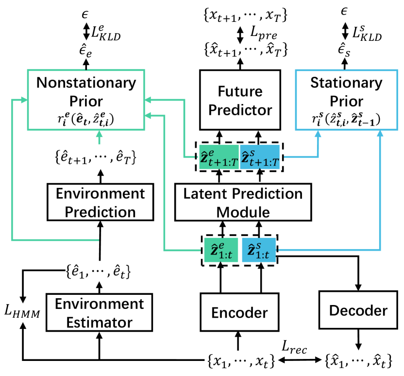
Figure 3: The framework of the Identifying Disentnagled Latent State model. The latent variable encoder is used to extract ${\mathbf{z}}^{s}_{1:t}$ and ${\mathbf{z}}^{e}_{1:t}$ from ${\mathbf{x}}_{1:t}$. The latent forecasting module is used to estimate ${\mathbf{z}}^{s}_{t+1:T}$ and ${\mathbf{z}}^{e}_{t+1:T}$ from ${\mathbf{z}}^{s}_{1:t}$ and ${\mathbf{z}}^{e}_{1:t}$, respectively. And the future forecasting module is used for future prediction $\{\hat{x}_{t+1},\cdots,\hat{x}_{T}\}$. The historical latent environments $\{\hat{{\mathbf{e}}}_{1},\cdots,\hat{{\mathbf{e}}}_{t}\}$ are generated by the environment estimation module, and the future latent environments $\{\hat{{\mathbf{e}}}_{t+1},\cdots,\hat{{\mathbf{e}}}_{T}\}$ are generated by the environment prediction module. The nonstationary prior and the stationary prior are used to estimate the prior distribution of stationary and nonstationary latent variables for KL divergence.

4.1 Sequential Variational Inference Module for Time Series Data Modeling

According to the data generation process in Figure 2, we first derive the evidence lower bound (ELBO) as shown in Equation (7). Please refer to Appendix D for more details on the derivation of the ELBO.

$$\small\begin{split}ELBO=&\mathcal{L}_{pre}\!+\!\alpha\mathbb{E}_{q({\mathbf{z}}^{e}_{1:t}|{\mathbf{x}}_{1:t}\!)}\mathbb{E}_{q({\mathbf{z}}^{s}_{1:t}|{\mathbf{x}}_{1:t}\!)}\mathcal{L}_{rec}\\ &\!-\!\beta\mathcal{L}_{KLD}^{s}\!-\!\gamma\mathcal{L}_{KLD}^{e}\end{split}$$ (7)

where $\alpha,\beta$ and $\gamma$ denote the hyper-parameters. Note that $\mathcal{L}_{rec}$ and $\mathcal{L}_{pre}$ denote the reconstruction of historical observations and future predictor module shown as follows:

$$\small\begin{split}\mathcal{L}_{rec}\!=&\mathbb{E}_{q({\mathbf{z}}^{e}_{1:t}|{\mathbf{x}}_{1:t})}\mathbb{E}_{q({\mathbf{z}}^{s}_{1:t}|{\mathbf{x}}_{1:t})}\ln p({\mathbf{x}}_{1:t}|{\mathbf{z}}^{e}_{1:t},{\mathbf{z}}^{s}_{1:t})\\ \mathcal{L}_{pre}\!=&\mathbb{E}_{q({\mathbf{z}}^{e}_{t:T}|{\mathbf{z}}^{e}_{1:t})}\mathbb{E}_{q({\mathbf{z}}^{s}_{t:T}|{\mathbf{z}}^{s}_{1:t})}\ln p({\mathbf{x}}_{t+1:T}|{\mathbf{z}}^{e}_{t+1:T},{\mathbf{z}}^{s}_{t+1:T}).\end{split}$$ (8)

$\mathcal{L}_{KLD}^{s}$ and $\mathcal{L}_{KLD}^{e}$ denote the Kullback-Leibler divergence between the approximated posterior distribution and the estimated prior distribution as shown in Equation (9):

$$\small\begin{split}\mathcal{L}_{KLD}^{s}\!=&D_{KL}\!(q({\mathbf{z}}^{s}_{1:t}|{\mathbf{x}}_{1:t})||p({\mathbf{z}}^{s}_{1:t}))\\ +&\mathbb{E}_{q({\mathbf{z}}^{s}_{1:t}|{\mathbf{x}}_{1:t})}\!\Big{[}\!D_{KL}\!(q({\mathbf{z}}^{s}_{t+1:T}|{\mathbf{z}}^{s}_{1:t})||p({\mathbf{z}}^{s}_{t+1:T}|{\mathbf{z}}^{s}_{1:t}))\Big{]}\\ \mathcal{L}_{KLD}^{e}\!=&D_{KL}\!(q({\mathbf{z}}^{e}_{1:t}|{\mathbf{x}}_{1:t})||p({\mathbf{z}}^{e}_{1:t}))\\ +&\mathbb{E}_{q({\mathbf{z}}^{e}_{1:t}|{\mathbf{x}}_{1:t})}\!\Big{[}\!D_{KL}\!(q({\mathbf{z}}^{e}_{t+1:T}|{\mathbf{z}}^{e}_{1:t})||p({\mathbf{z}}^{e}_{t+1:T}|{\mathbf{z}}^{e}_{1:t}))\Big{]},\end{split}$$ (9)

in which $q({\mathbf{z}}_{1:t}^{s}|{\mathbf{x}}_{1:t}),\,\,q({\mathbf{z}}_{t+1:T}^{s}|{\mathbf{z}}_{1:t}^{s}),\,\,q({\mathbf{z}}_{1:t}^{e}|{\mathbf{x}}_{1:t})$ and $q({\mathbf{z}}_{t+1:T}^{e}|{\mathbf{z}}_{1:t}^{e})$ are used to approximate the distribution; Therefore, the aforementioned approximated functions, historical decoder, and the future forecasting module can be formalized as follows:

$$\small\begin{split}{\mathbf{z}}^{e}_{1:t}&=\psi_{e}({\mathbf{x}}_{1:t};\theta_{\psi_{e}}),\quad\quad\,\,\,\,\quad{\mathbf{z}}^{s}_{1:t}=\psi_{s}({\mathbf{x}}_{1:t};\theta_{\psi_{s}}),\\ {\mathbf{z}}^{e}_{t+1:T}&=T_{e}({\mathbf{z}}^{e}_{1:t};\theta_{T_{e}}),\,\,\,\,\quad\quad{\mathbf{z}}^{s}_{t+1:T}=T_{s}({\mathbf{z}}^{s}_{1:t};\theta_{T_{s}}),\\ \hat{{\mathbf{x}}}_{1:t}&=F_{x}({\mathbf{z}}^{e}_{1:t},{\mathbf{z}}^{s}_{1:t};\theta_{x}),\quad\hat{{\mathbf{x}}}_{t+1:T}=F_{y}({\mathbf{z}}^{e}_{t+1:T},{\mathbf{z}}^{s}_{t+1:T};\theta_{y}),\end{split}$$ (10)

where $\psi_{s},\psi_{e}$ denote the latent variable encoder of stationary and nonstationary latent variables; $T_{s},T_{e}$ are latent prediction modules; and $F_{x},F_{y}$ denote the decoder of historical observations and the future forecasting module, respectively, which are all implemented by Multi-layer Perceptron networks (MLPs); and $\theta_{\psi_{e}},\theta_{\psi_{s}},\theta_{T_{e}},\theta_{T_{s}}$, and $\theta_{x},\theta_{y}$ are the trainable parameters of neural networks.

$p({\mathbf{z}}^{s}_{1:t}),\,\,p({\mathbf{z}}^{s}_{t+1:T}|{\mathbf{z}}^{s}_{1:t}),\,\,p({\mathbf{z}}^{e}_{1:t})$ and $p({\mathbf{z}}^{e}_{t+1:T}|{\mathbf{z}}^{e}_{1:t})$ are the estimated prior distribution of stationary and nonstationary latent variables, which will be introduced in the subsection 4.2. Note that the environment estimation module does not appear in the ELBO explicitly, which is a part of the $p({\mathbf{z}}^{e}_{1:t}),p({\mathbf{z}}^{e}_{t+1:T}|{\mathbf{z}}^{e}_{1:t})$ and will be also introduced in subsection 4.2. Please refer to the Appendix H for more details of the implementation of the proposed IDEA model.

4.2 Modular Architectures with Stationary and Nonstationary Priors

Previous time-series modeling methods based on the causality-based data generation processes usually require autoregressive inference and Gaussian prior (Fabius & Van Amersfoort, 2014; Kim et al., 2019; Zhu et al., 2020). However, these prior distributions usually contain temporal information and follow an unknown distribution. Simply assuming the Gaussian distribution might result in suboptimal performance of disentanglement. To solve this problem, we employ the modular neural architecture to estimate the prior distribution of stationary and nonstationary latent variables.

Modular Architecture for the Stationary Prior Estimation. we first let $\{r_{i}^{s}\}$ be a set of learned inverse transition functions that take the estimated stationary latent variables and output the noise term, i.e., $\hat{\epsilon}_{t,i}^{s}=r_{i}^{s}(\hat{z}_{t,i}^{s},\hat{{\mathbf{z}}}^{s}_{t-1})$ and each $r_{i}^{s}$ is modeled with MLPs. Then we devise a transformation $\phi^{s}:=\{\hat{{\mathbf{z}}}^{s}_{t-1},\hat{{\mathbf{z}}}^{s}_{t}\}\rightarrow\{\hat{{\mathbf{z}}}^{s}_{t-1},\hat{\epsilon}^{s}_{t}\}$, and its Jacobian is $\small{\mathbf{J}_{\phi^{s}}=\begin{pmatrix}\mathbb{I}&0\\ *&\text{diag}\left(\frac{\partial r^{s}_{i}}{\partial\hat{z}_{t-1,i}^{s}}\right)\end{pmatrix}}$, where $*$ denotes a matrix. By applying the change of variables formula, we have the following equation:

$$\small\log p(\hat{{\mathbf{z}}}^{s}_{t-1},\hat{{\mathbf{z}}}^{s}_{t})=\log p(\hat{{\mathbf{z}}}^{s}_{t-1},\hat{\epsilon}_{t}^{s})+\log|\text{det}(\mathbf{J}_{\phi})|.$$ (11)

Since we assume that the noise term in Equation (2) is independent with ${\mathbf{z}}_{t-1}^{s}$, we enforce the independence of the estimated noise $\hat{\epsilon}_{t}^{s}$ and we further have:

$$\small\log p(\hat{{\mathbf{z}}}^{s}_{t}|{\mathbf{z}}^{s}_{t-1})=\log p(\hat{\epsilon}^{s}_{t})+\sum_{i=n_{d}+1}^{n}\log|\frac{\partial r_{i}^{s}}{\partial\hat{z}^{s}_{t-1,i}}|.$$ (12)

Therefore, the stationary prior can be estimated as follows:

$$\small p(\hat{{\mathbf{z}}}_{1:t}^{s})=p(\hat{{\mathbf{z}}}^{s}_{1})\prod_{\tau=2}^{t}\!\!\left(\sum_{i=n_{d}+1}^{n}\log p(\hat{\epsilon}^{s}_{\tau,i})+\!\!\!\!\sum_{i=n_{d}+1}^{n}\!\!\!\log|\frac{\partial r_{i}^{s}}{\partial\hat{z}^{s}_{\tau-1,i}}|\right),$$ (13)

where $p(\hat{\epsilon}^{s}_{i})$ follow Gaussian distributions. And another prior $p(\hat{{\mathbf{z}}}_{t+1:T}^{s}|\hat{{\mathbf{z}}}_{1:t}^{s})$ follows a similar derivation.

Modular Architecture for the Nonstationary Prior Estimation. We employ a similar derivation and let $\{r_{i}^{e}\}$ be a set of learned inverse transition functions, which take the estimated environment labels $\hat{{\mathbf{e}}}_{t}$ and $\hat{{\mathbf{z}}}^{e}_{t}$ as input and output the noise term, i.e. $\hat{\epsilon}^{e}_{t}=r_{i}^{e}(\hat{{\mathbf{e}}}_{t},\hat{z}^{e}_{t,i})$.

Leaving $r_{i}^{e}$ be an MLP, we further devise another transformation $\phi^{e}:=\{\hat{{\mathbf{e}}}_{t},\hat{{\mathbf{z}}}^{e}_{t}\}\rightarrow\{\hat{{\mathbf{e}}}_{t},\hat{\epsilon}^{e}_{t}\}$ with its Jacobian is $\small{\mathbf{J}_{\phi^{e}}=\begin{pmatrix}\mathbb{I}&0\\ *&\text{diag}\left(\frac{\partial r_{i}^{e}}{\partial\hat{z}_{t,i}^{e}}\right)\end{pmatrix}}$, where $*$ denotes a matrix. Similar to the derivation of stationary prior, we have:

$$\small\ln p(\hat{{\mathbf{z}}}_{t}^{e}|\hat{{\mathbf{e}}}_{t})=\ln p(\hat{\epsilon}^{e}_{t})+\sum_{i=1}^{n_{e}}\ln|\frac{\partial r_{i}^{e}}{\partial\hat{z}^{e}_{t,i}}|.$$ (14)

Therefore, the nonstationary prior can be estimated by maximizing the following equation:

$$\small\begin{split}\ln p({\mathbf{z}}^{e}_{1:t})&=\mathbb{E}_{q(\hat{{\mathbf{e}}}_{1:t})}\sum_{\tau=1}^{t}\left(\sum_{i=1}^{n_{e}}\ln p(\hat{\epsilon}^{e}_{\tau,i})+\sum_{i=1}^{n_{e}}\ln|\frac{\partial r_{i}^{e}}{\partial\hat{z}^{e}_{\tau,i}}|\right).\end{split}$$ (15)

Note that $q(\hat{{\mathbf{e}}}_{1:t})$ denotes the environment estimation module, which is implemented with an autoregressive hidden Markov model and generates latent environment indices with the help of the Viterbi algorithm (Song et al., 2023; Elliott et al., 2012). To optimize the autoregressive hidden Markov model, we need to maximize its free energy lower bound, which is shown as follows:

$$\small\begin{split}\ln p({\mathbf{x}}_{1:t})=&\mathbb{E}_{q({\mathbf{e}}_{1:t})}\ln\frac{p({\mathbf{x}}_{1:t},{\mathbf{e}}_{1:t})q({\mathbf{e}}_{1:t})}{p({\mathbf{e}}_{1:t}|{\mathbf{x}}_{1:t})q({\mathbf{e}}_{1:t})}\\ \geq&\mathbb{E}_{q({\mathbf{e}}_{1:t})}p({\mathbf{e}}_{1:t}|{\mathbf{x}}_{1:t})-\textbf{H}(q({\mathbf{e}}_{1:t}))=\mathcal{L}_{HMM}.\end{split}$$ (16)

Please refer to more detailed derivations of stationary and nonstationary in Appendix C.

4.3 Model Summary

Considering that the autoregressive hidden Markov model converges much faster than the sequential variational inference model, we employ a two-phase training strategy. Specifically, we first minimize $\mathcal{L}_{HMM}$ to train the autoregressive hidden Markov model. Sequentially, we minimize $\mathcal{L}_{EBLO}$ by fixing the parameters of the autoregressive hidden Markov model. Since we use the historical observations ${\mathbf{x}}_{1:t}$ to generate $\hat{{\mathbf{e}}}_{1:t}$, which can be used to estimate the transition matrix $\hat{\mathbf{A}}$, during testing phase, we can estimate $\hat{{\mathbf{e}}}_{t+1:T}$ by sampling from $\hat{\mathbf{A}}$ as shown in the environment prediction block in Figure 3.

4.4 Complexity Analysis

We further provide time complexity for the IDEA model. We first let $L$ be the length of the time series and the model complexity depends on the autoregress hidden Markov model and the sequential variational inference model. First, suppose that $\bm{\mathrm{E}}$ is the number of latent environments, then the complexity of the autoregress hidden Markov model is $\mathcal{O}(\bm{\mathrm{E}}L)$. Moreover, suppose that $n$ is the number of latent variables, then the complexity of the sequential variational inference model is $\mathcal{O}(nL)$. In practice, the number of latent environments and the dimension of latent variables are low, so our model enjoys an efficient computation. Please refer to Appendix G for model efficiency comparison from the perspectives of performance, efficiency, and GPU memory.

5 Experiments

5.1 Synthetic Experiments

5.1.1 Experimental Setup

Data Generation. We generate the simulated nonstationary time series data with 3 environments as mentioned in Figure 2 and Equation (1)-(3). Specifically, we first randomly initialized a Markov Chain with a transition matrix A. Sequentially, for each environment, we consider different Gaussian distributions and generate the nonstationary latent variables ${\mathbf{z}}_{t}^{e}$. As for the stationary latent variables, we employ an MLP with a LeakyReLU unit as the transition function. Note that we generate Dataset A and Dataset B with different time lag dependencies. Finally, we use a randomly initialized MLP to generate the observation data.

Evaluation Metrics. We consider three different metrics to evaluate the effectiveness of our method. First, to evaluate the identifiability of the stationary and nonstationary latent variables, consider the Mean Correlation Coefficient (MCC) on the test dataset, which is a standard metric for nonlinear ICA. A higher MCC denotes a better identification performance the model can achieve. Second, to evaluate the identifiability of the transition matrix A, we further consider the Mean Square Error (MSE) between the ground truth A and the estimated one. A lower value of MSE implies the model can identify the transition matrix better. Finally, we also consider the accuracy of ${\mathbf{e}}_{t}$ estimation since it reflects the performance of our model in detecting when the temporal distribution shift occurs. Please refer to Appendix F.1 for a detailed discussion about evaluation metrics.

Baselines. Besides the standard BetaVAE (Higgins et al., 2016) that does not consider any temporal and environment information, we also take some conventional nonlinear ICA methods into account like TCA (Hyvarinen & Morioka, 2016)and i-VAE (Khemakhem et al., 2020a). Moreover, we consider TDRL (Yao et al., 2022), which considers stationary and nonstationary causal dynamics, but requires observed environment variables. Finally, we consider the HMNLICL (Hälvä & Hyvarinen, 2020) and NCTRL (Song et al., 2023), which assume that the environment variables are latent but follow a Markov Chain.

5.1.2 Results and Discussion

Table 1: Experiment results of two synthetic datasets on baselines and proposed IDEA.

Method	Mean Correlation Coefficien (MCC)
	Dataset A	Dataset B	Average
BetaVAE (Higgins et al., 2016)	64.2	63.2	63.7
TCL (Hyvarinen & Morioka, 2016)	56.0	65.8	60.9
i-VAE (Khemakhem et al., 2020a)	76.9	73.0	74.9
HMNLICA (Hälvä & Hyvarinen, 2020)	83.2	74.5	78.8
TDRL (Yao et al., 2022)	78.5	78.8	78.6
NCTRL (Song et al., 2023)	81.4	79.4	80.4
IDEA	97.5	92.7	95.1

We generate two different synthetic datasets with different time lags dependencies. Experiment results of MCC are shown in Table 1, and the experiment results of environment estimation accuracy and MSE can be found in Appendix F.1. According to the experiment results, we can draw the following conclusions: 1) We can find that the accuracies of environment estimation are high in both two datasets. Since the Dataset B contains more complex temporal relationships, the corresponding accuracy is slightly lower. 2) We can also find that the proposed IDEA model can reconstruct the latent variables under unknown temporal distribution shift with ideal MCC performance, i.e., $(>0.95)$ on average. In the meanwhile, the other compared methods, that do not use historical dependency, can hardly perform well. Moreover, the TDRL, which considers the temporal causal relationship, cannot obtain an ideal MCC performance since it requires observed environments. 3) Although baselines like HMNLICA and NCTRL assume latent environments on a Markov Chain, they perform worse than our IDEA. This is because both HMNLICA and NCTRL do not consider the stationary and nonstationary latent variables in the data generation process simultaneously.

Table 2: MSE and MAE results on the ETTh1, ETTh2, Exchange, ILI, Weather, Traffic, and ECL datasets. N-Transformer denotes the nonstationary Transformer due to the limited space.

Models		IDEA		Koopa		SAN		DLinear		N-Transformer		RevIN		MICN		TimeNets		WITRAN
Metric		MSE	MAE	MSE	MAE	MSE	MAE	MSE	MAE	MSE	MAE	MSE	MAE	MSE	MAE	MSE	MAE	MSE	MAE
ETTh1	36-12	0.291	0.345	0.323	0.370	0.624	0.522	0.330	0.368	0.387	0.409	0.372	0.408	0.292	0.358	0.350	0.389	0.329	0.375
	72-24	0.300	0.353	0.305	0.356	0.319	0.376	0.312	0.355	0.469	0.449	0.402	0.425	0.324	0.378	0.343	0.390	0.340	0.388
	144-48	0.338	0.38	0.353	0.388	0.367	0.406	0.351	0.380	0.548	0.507	0.458	0.445	0.396	0.418	0.376	0.407	0.385	0.419
	216-72	0.367	0.388	0.379	0.404	0.462	0.457	0.372	0.394	0.606	0.536	0.494	0.468	0.396	0.429	0.409	0.430	0.410	0.436
ETTh2	36-12	0.141	0.236	0.142	0.240	0.160	0.271	0.161	0.269	0.156	0.256	0.177	0.274	0.148	0.255	0.152	0.251	0.143	0.248
	72-24	0.173	0.260	0.185	0.271	0.343	0.413	0.187	0.285	0.216	0.301	0.266	0.340	0.183	0.280	0.194	0.284	0.180	0.276
	144-48	0.233	0.306	0.243	0.313	0.266	0.337	0.240	0.321	0.309	0.378	0.380	0.417	0.253	0.335	0.270	0.336	0.256	0.329
	216-72	0.262	0.327	0.283	0.344	0.301	0.367	0.287	0.356	0.396	0.426	0.442	0.457	0.294	0.362	0.307	0.363	0.312	0.368
Exchange	36-12	0.014	0.074	0.015	0.079	0.014	0.074	0.016	0.088	0.017	0.085	0.022	0.102	0.018	0.093	0.016	0.084	0.014	0.075
	72-24	0.023	0.102	0.027	0.113	0.024	0.105	0.026	0.110	0.031	0.122	0.045	0.152	0.027	0.115	0.031	0.123	0.025	0.107
	144-48	0.042	0.141	0.050	0.156	0.046	0.153	0.049	0.160	0.077	0.196	0.127	0.261	0.045	0.153	0.072	0.194	0.046	0.148
	216-72	0.065	0.180	0.075	0.193	0.066	0.186	0.071	0.189	0.123	0.252	0.233	0.357	0.064	0.183	0.115	0.251	0.071	0.185
ILI	36-12	1.218	0.694	1.994	0.880	2.296	1.027	2.620	1.154	1.491	0.757	2.637	1.094	4.847	1.570	2.406	0.840	2.138	0.914
	72-24	1.680	0.809	2.077	0.919	2.472	1.074	2.733	1.177	2.551	1.039	2.653	1.116	4.776	1.556	2.270	0.988	2.867	1.080
	108-36	1.792	0.869	1.836	0.881	3.228	1.209	2.271	1.094	2.227	1.018	2.696	1.139	4.917	1.584	2.978	1.123	3.147	1.151
	144-48	1.883	0.926	2.072	0.941	3.842	1.280	2.490	1.187	2.595	1.081	2.960	1.167	4.804	1.584	2.696	1.098	3.388	1.232
weather	36-12	0.072	0.09	0.076	0.098	0.079	0.121	0.080	0.127	0.077	0.100	0.095	0.127	0.076	0.120	0.081	0.106	0.093	0.144
	72-24	0.098	0.130	0.100	0.133	0.109	0.160	0.113	0.172	0.110	0.145	0.134	0.193	0.099	0.150	0.110	0.151	0.143	0.203
	144-48	0.115	0.158	0.125	0.164	0.128	0.181	0.130	0.193	0.138	0.187	0.175	0.237	0.127	0.186	0.131	0.178	0.202	0.262
	216-72	0.136	0.187	0.139	0.187	0.148	0.210	0.147	0.215	0.174	0.225	0.225	0.287	0.149	0.213	0.149	0.202	0.271	0.319
ECL	36-12	0.114	0.216	0.135	0.245	0.133	0.246	0.166	0.254	0.134	0.242	0.136	0.254	0.250	0.338	0.128	0.236	0.147	0.272
	72-24	0.121	0.220	0.129	0.236	0.139	0.252	0.166	0.252	0.14	0.246	0.144	0.257	0.258	0.342	0.134	0.242	0.155	0.278
	144-48	0.122	0.224	0.136	0.242	0.148	0.259	0.151	0.245	0.155	0.260	0.163	0.275	0.271	0.353	0.149	0.256	0.172	0.291
	216-72	0.131	0.232	0.142	0.246	0.156	0.264	0.144	0.242	0.169	0.274	0.175	0.287	0.279	0.357	0.166	0.271	0.183	0.300
Traffic	36-12	0.457	0.300	0.472	0.312	0.489	0.304	0.602	0.381	0.626	0.319	0.567	0.373	0.583	0.312	0.609	0.306	0.802	0.387
	72-24	0.458	0.305	0.450	0.309	0.495	0.310	0.613	0.386	0.574	0.310	0.548	0.363	0.618	0.334	0.553	0.296	0.811	0.401
	144-48	0.410	0.283	0.420	0.302	0.489	0.309	0.472	0.319	0.590	0.330	0.570	0.361	0.616	0.327	0.555	0.301	0.830	0.406
	216-72	0.403	0.277	0.424	0.308	0.500	0.312	0.441	0.300	0.604	0.338	0.547	0.336	0.650	0.343	0.577	0.311	0.854	0.415

5.2 Real-world Experiments

5.2.1 Experiment Setup

Datasets. To evaluate the effectiveness of our IDEA method in real-world scenarios, we conduct experiments on eight real-world benchmark datasets that are widely used in nonstationary time series forecasting: ETT (Zhou et al., 2021), Exchange (Lai et al., 2018), ILI(CDC), electricity consuming load (ECL), weather (Wetterstation), traffic and M4 (Makridakis et al., 2020). More detailed descriptions of the datasets can be referred to Appendix F.2.1. We employ the same data preprocessing and split ratio in TimeNet (Wu et al., 2022). Similarly to Koopa (Liu et al., 2023b), for each forecasting window length $H$, we let the length of the lookback window $3H$ to make sure that each type of environment exists in the lookback window. Moreover, for each dataset, we consider different forecast lengths $H\in\{12,24,48,72\}$.

Baselines. To evaluate the effectiveness of the proposed IDEA, we consider the following state-of-the-art deep forecasting models for time series data. First, we consider the methods for long-term forecasting including the TCN-based methods like TimesNet (Wu et al., 2022) and MICN (Wang et al., 2022), the MLP-based methods like DLinear (Zeng et al., 2023), as well as the recently proposed WITRAN (Jia et al., 2023). Moreover, we further consider the methods with the assumption that the temporal distribution shift occurs among instances like RevIN (Kim et al., 2021) and Nonstationary Transformer (Liu et al., 2022). Finally, we compare the nonstationary forecasting methods with the assumption that temporal distribution shift occurs uniformly in each instance, like Koopa (Liu et al., 2023b) and SAN (Liu et al., 2023c). Since SAN is a framework that boosts other forecasting models, we report the results of SAN+autoformer (Wu et al., 2021). We repeat each experiment over 3 random seeds and publish the average performance.

Experiment Details. We use ADAM optimizer (Kingma & Ba, 2014) in all experiments and report the mean squared error (MSE) and the mean absolute error (MAE) as evaluation metrics. All experiments are implemented by Pytorch on a single NVIDIA RTX A5000 24GB GPU.

5.2.2 Results and Discussion

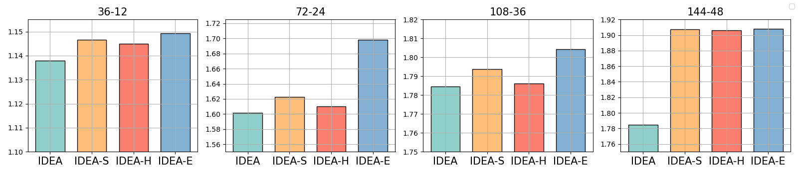
Figure 4: Ablation study on the different predict forecast lengths of ILI dataset. we explore the impact of different loss terms.

Quantitative Results. Experiment results on each dataset are shown in Table 2. Please refer to Appendix F.2.2 and F.3 for experiment results on other datasets and sensitive analyis. According to the experiment results, our IDEA model significantly outperforms all other baselines on most forecasting tasks. Specifically, our method outperforms the most competitive baselines by a clear margin of $1.7\%-12\%$ and reduces the forecasting errors substantially on some hard benchmarks, e.g., weather and ILI. Besides outperforming the forecasting model without the nonstationary assumptions like TimesNet and DLinear, our IDEA model also outperforms those methods for nonstationary time series data like RevIN and nonstationary Transformer. However, our method achieves the second-best but still comparable results in the Exchange dataset of the forecasing length of 72, this might be caused by the inaccurate environment estimation for long-term prediction.

It is remarkable that our method achieves a better performance than that of Koopa and SAN, which assume temporal distribution shifts in each time series instance. This is because these methods assume that uniform temporal distribution shifts in each time series instance, which is hard to meet in real-world scenarios, and it is hard for these methods to disentangle the stationary and nonstationary components simultaneously. Meanwhile, our method detects when the temporal distribution shift occurs and further disentangles the stationary and nonstationary states with identification guarantees, hence it can achieve the ideal nonstationary forecasting performance. Please refer to Appendix F.2.2 for experiment results on the M4 dataset.

5.2.3 Ablation Study

We further devise three model variants. a) IDEA-H: we remove the autoregressive hidden Markov model for environment estimation, and use random environment variables. b) IDEA-E: we remove the nonstationary prior and the corresponding KL divergence term. c) IDEA-S: we remove the stationary prior and the corresponding Kullback-Leibler divergence term. Experiment results on the ILI dataset are shown in Figure 4. We find that 1) the performance of IDEA-H drops without an accurate estimation of the environments, implying that the accurate environment estimation benefits the disentanglement and forecasting performance. 2) Both stationary and non-stationary priors play an important role in non-stationary forecasting, indirectly implying that these priors can benefit the capture of temporal information and the nonstationary forecasting performance.

6 Conclusion

This paper presents a general data generation process for nonstationary time series forecasting, aligning closely with real-world scenarios. Based on this data generation process, we establish the identifiability of latent stationary latent variables, and nonstationary latent variables via sufficient observation. This contribution stands as a groundbreaking and theoretically sound solution for nonstationary time-series forecasting. Compared with the existing methods, our IDEA model breaks the strong assumption of uniform temporal distribution shifts, making it possible to apply our method to real-world data. Experiment results on several mainstream benchmark datasets further evaluate the effectiveness of our method. In summary, this paper represents a significant stride forward in the field of nonstationary time series forecasting and causal representation learning.

7 Impact Statement

The proposed IDEA model can detect when the temporal distribution shifts occur and disentangle the stationary and nonstationary latent variables. Therefore, our IDEA could be applied to a wide range of applications including time series forecasting, imputation, and classification. Specifically, the disentangled stationary and nonstationary latent variables would create a model that is more transparent, thereby aiding in the reduction of bias and the promotion of fairness of the existing time series forecasting models.

Appendix A Related Works

We review the works about nonstationary time series forecasting and the identifiability of latent variables.

Nonstationary Time Series Forecasting. Time series forecasting is a conventional task in the field of machine learning with lots of successful cases, e.g, autoregressive model (Hyndman & Athanasopoulos, 2018) and ARMA (Box & Pierce, 1970). Previously, deep neural networks also have made great contributions to time series forecasting, e.g., RNN-based models (Hochreiter & Schmidhuber, 1997; Lai et al., 2018; Salinas et al., 2020), CNN-based models (Bai et al., 2018; Wang et al., 2022; Wu et al., 2022), and the methods based on state-space model (Gu et al., 2022, 2020, 2021b, 2021a; Smith et al., 2022). Recently, transformer-based methods (Zhou et al., 2021; Wu et al., 2021; Liu et al., 2023a; Nie et al., 2022) have boosted the development of time series forecasting. However, these methods are devised for stationary time series, so nonstationary forecasting is receiving more and more attention. One straightforward solution to this challenge is to discard the nonstationarity via preprocessing methods like stationarization (Virili & Freisleben, 2000) and differencing (Salles et al., 2019), but they might destroy the temporal dependency. Recent studies have used two different assumptions to further solve this problem. By assuming that the temporal distribution shift occurs among datasets and each sequence instance is stationary (Cai et al., 2021; Eldele et al., 2023), some methods consider normalization-based methods. Kim et.al (Kim et al., 2021) propose the reversible instance normalization to remove and restore the statistical information of a time-series instance. Liu et.al (Liu et al., 2022) propose the nonstationary Transformer, which includes the destationary attention mechanism to recover the intrinsic non-stationary information into temporal dependencies. By assuming that the temporal distribution shift uniformly occurs in each sequence instance and so each equal-size segmentation is stationary, other methods propose to disentangle the stationary and nonstationary components. Surana et.al (Surana, 2020) and Liu et.al (Liu et al., 2023b) employ the Koopman theory (Korda & Mezić, 2018), which transform the nonlinear system into several linear operators, to decompose the stationary and nonstationary factors. Liu et.al (Liu et al., 2023c) use adaptive normalization and denormlization on non-overlap equally-sized slices. However, since the temporal distribution shift may occur any time, the aforementioned two assumptions are unreasonable. To solve this problem with milder assumptions, the proposed IDEA first identifies when the distribution shift occurs and then identifies the latent states to learn how they change over time with the help of Markov assumption of latent environment and sufficient observation assumption.

Identifiability of Latent Variables. Identifiability of latent variables (Kong et al., 2023b; Yan et al., 2023; Kong et al., 2023a) plays a significant role in the explanation and generalization of deep generative models, guaranteeing that causal representation learning can capture the underlying factors and describe the latent generation process (Kumar et al., 2017; Locatello et al., 2019a, b; Schölkopf et al., 2021; Träuble et al., 2021; Zheng et al., 2022). Several researchers employ independent component analysis (ICA) to learn causal representation with identifiability (Comon, 1994; Hyvärinen, 2013; Lee & Lee, 1998; Zhang & Chan, 2007) by assuming a linear generation process. To extend it to the nonlinear scenario, different extra assumptions about auxiliary variables or generation processes are adopted to guarantee the identifiability of latent variables (Zheng et al., 2022; Hyvärinen & Pajunen, 1999; Hyvärinen et al., 2023; Khemakhem et al., 2020b; Li et al., 2023c). Previously, Aapo et.al established the identification results of nonlinear ICA by introducing auxiliary variables e.g., domain indexes, time indexes, and class labels(Khemakhem et al., 2020a; Hyvarinen & Morioka, 2016, 2017; Hyvarinen et al., 2019). However, these methods usually assume that the latent variables are conditionally independent and follow the exponential families distributions. Recently, Zhang et.al release the exponential family restriction (Kong et al., 2022; Xie et al., 2022) and propose the component-wise identification results for nonlinear ICA with a certain number of auxiliary variables. They further propose the subspace Identification (Li et al., 2023a) for multi-source domain adaptation, which requires fewer auxiliary variables. In the field of sequential data modeling, Yao et.al (Yao et al., 2021, 2022) recover time-delay latent dynamics and identify their relations from sequential data under the stationary environment and different distribution shifts. And Lippe et.al propose the (i)-CITRIS (Lippe et al., 2022b, a), which use intervention target information for identifiability of scalar and multidimensional latent causal factors. Moreover, Hälvä et.al (Hälvä & Hyvarinen, 2020) and Song et.al (Song et al., 2023) utilize the Markov assumption to provide identification guarantee of time series data without extra auxiliary variables. Although Yao et.al (Yao et al., 2022) partitioned the latent space into stationary and nonstationary parts, they require extra environment variables. Furthermore, although Hälvä et.al (Hälvä & Hyvarinen, 2020) and Song et.al (Song et al., 2023) provide identifiability results without extra environment variables, they can hardly disentangle the stationary and nonstationary, respectively. In this paper, we provide a causal generation process for nonstationary time series data, where the observations are generated by the environment-irrelated stationary latent variables and environment-related nonstationary latent variables. To show the identifiability of these latent variables, we employ the Markov assumption of latent environments and the extension of Kruskal’s theorem (Allman et al., 2009; Kruskal, 1977, 1976) to identify the latent discrete environment variables. Moreover, to disentangle the stationary and nonstationary latent states, we employ the sufficient observation assumption, which requires at least 2 consecutive observations for each latent environment and is reasonable in nonstationary time series, so the symmetry of the stationary and nonstationary latent variables is broken, making it possible to disentangle these latent variables. Summarization and differences of the recent literature related to our work from six different perspectives are shown in Table 3.

Table 3: Summarization and different of the existing identification based on nonlinear ICA. A green check denotes that a method has an attribute, whereas a red cross denotes the opposite.

Theory	Time-varying Relation	Causally-related Process	Partitioned Subspace	Unknown Environments	Subspace Identification
TCL (Hyvarinen & Morioka, 2016)	✔	✗	✗	✗	✗
PCL (Hyvarinen & Morioka, 2017)	✔	✗	✗	✗	✗
HM-NLICA (Hälvä & Hyvarinen, 2020)	✔	✗	✗	✔	✗
i-VAE (Khemakhem et al., 2020a)	✗	✗	✗	✗	✗
LEAP (Yao et al., 2021)	✔	✔	✗	✗	✗
TDRL (Yao et al., 2022)	✔	✔	✔	✗	✗
SIG (Li et al., 2023a)	✗	✗	✔	✗	✔
NCTRL (Song et al., 2023)	✔	✔	✗	✔	✗
IDEA	✔	✔	✔	✔	✔

Appendix B Identification

In this section, we provide the definition of different types of identificaiton.

B.1 Componenet-wise Identification

For each ground-truth changing latent variables $z_{t,i}$, there exists a corresponding estimated component $\hat{z}_{t,j}$ and an invertible function $h_{t,i}:\mathbb{R}\rightarrow\mathbb{R}$, such that $\hat{z}_{t,j}=h(z_{t,i})$.

B.2 Subspace Identification

For each ground-truth changing latent variables $z_{t,i}$, the subspace identification means that there exists $\hat{{\mathbf{z}}}_{t}$ and an invertible function $z_{t,i}=h_{i}(\hat{{\mathbf{z}}}_{t})$, such that $z_{t,i}=h_{i}(\hat{{\mathbf{z}}}_{t})$.

B.3 Identification Up to Label Swapping

If $\tilde{\textbf{A}}$ is a $E\times E$ transition matrix and if $\tilde{\pi}(e)$ is a stationary distribution of $\tilde{\textbf{A}}$ with $\tilde{\pi}(e)>0,\forall e\in\{1,\cdots,E\}$ and if $\tilde{M}=\{\tilde{\mu}_{1},\cdots,\tilde{\mu}_{j},\cdots,\tilde{\mu}_{E}\}$ are $E$ probability distributions that verify the equality of the distribution functions $\mathbb{P}^{(3)}_{\tilde{\textbf{A}},\tilde{M}}=\mathbb{P}^{(3)}_{{\textbf{A}},{M}}$, then there exist a permutation $\sigma$ of set $\{1,\cdots,E\}$ such that for all $k,l=1,\cdots,E$, we have $\tilde{A}_{k.l}=A_{\sigma(k),\sigma(l)}$ and $\tilde{\mu}_{k}=\mu_{\sigma(k)}$.

Appendix C Prior Likelihood Derivation

In this section, we derive the prior of $p(\hat{{\mathbf{z}}}_{1:t}^{s})$ and $p(\hat{{\mathbf{z}}}_{1:t}^{e})$ as follows:

• We first consider the prior of $\ln p({\mathbf{z}}_{1:t}^{s})$. We start with an illustrative example of stationary latent causal processes with two time-delay latent variables, i.e. ${\mathbf{z}}^{s}_{t}=[z^{s}_{t,1},z^{s}_{t,2}]$ with maximum time lag $L=1$, i.e., $z_{t,i}^{s}=f_{i}({\mathbf{z}}_{t-1}^{s},\epsilon_{t,i}^{s})$ with mutually independent noises. Then we write this latent process as a transformation map $\mathbf{f}$ (note that we overload the notation $f$ for transition functions and for the transformation map):

  $$\small\begin{gathered}\begin{bmatrix}\begin{array}[]{c}z_{t-1,1}^{s}\\ z_{t-1,2}^{s}\\ z_{t,1}^{s}\\ z_{t,2}^{s}\end{array}\end{bmatrix}=\mathbf{f}\left(\begin{bmatrix}\begin{array}[]{c}z_{t-1,1}^{s}\\ z_{t-1,2}^{s}\\ \epsilon_{t,1}^{s}\\ \epsilon_{t,2}^{s}\end{array}\end{bmatrix}\right).\end{gathered}$$

  By applying the change of variables formula to the map $\mathbf{f}$, we can evaluate the joint distribution of the latent variables $p(z_{t-1,1}^{s},z_{t-1,2}^{s},z_{t,1}^{s},z_{t,2}^{s})$ as

  $$\small p(z_{t-1,1}^{s},z_{t-1,2}^{s},z_{t,1}^{s},z_{t,2}^{s})=\frac{p(z_{t-1,1}^{s},z_{t-1,2}^{s},\epsilon_{t,1}^{s},\epsilon_{t,2}^{s})}{|\text{det }\mathbf{J}_{\mathbf{f}}|},$$ (17)

  where $\mathbf{J}_{\mathbf{f}}$ is the Jacobian matrix of the map $\mathbf{f}$, which is naturally a low-triangular matrix:

  $$\small\begin{gathered}\mathbf{J}_{\mathbf{f}}=\begin{bmatrix}\begin{array}[]{cccc}1&0&0&0\\ 0&1&0&0\\ \frac{\partial z_{t,1}^{s}}{\partial z_{t-1,1}^{s}}&\frac{\partial z_{t,1}^{s}}{\partial z_{t-1,2}^{s}}&\frac{\partial z_{t,1}^{s}}{\partial\epsilon_{t,1}^{s}}&0\\ \frac{\partial z_{t,2}^{s}}{\partial z_{t-1,1}^{s}}&\frac{\partial z_{t,2}^{s}}{\partial z_{t-1,2}^{s}}&0&\frac{\partial z_{t,2}^{s}}{\partial\epsilon_{t,2}^{s}}\end{array}\end{bmatrix}.\end{gathered}$$

  Given that this Jacobian is triangular, we can efficiently compute its determinant as $\prod_{i}\frac{\partial z_{t,i}^{s}}{\epsilon_{t,i}^{s}}$. Furthermore, because the noise terms are mutually independent, and hence $\epsilon_{t,i}^{s}\perp\epsilon_{t,j}^{s}$ for $j\neq i$ and $\epsilon_{t}^{s}\perp{\mathbf{z}}_{t-1}^{s}$, so we can with the RHS of Equation (17) as follows

  $$\small\begin{split}p(z_{t-1,1}^{s},z_{t-1,2}^{s},z_{t,1}^{s},z_{t,2}^{s})=p(z_{t-1,1}^{s},z_{t-1,2}^{s})\times\frac{p(\epsilon_{t,1}^{s},\epsilon_{t,2}^{s})}{|\mathbf{J}_{\mathbf{f}}|}=p(z_{t-1,1}^{s},z_{t-1,2}^{s})\times\frac{\prod_{i}p(\epsilon_{t,i}^{s})}{|\mathbf{J}_{\mathbf{f}}|}.\end{split}$$ (18)

  Finally, we generalize this example and derive the prior likelihood below. Let $\{r_{i}^{s}\}_{i=1,2,3,\cdots}$ be a set of learned inverse transition functions that take the estimated latent causal variables, and output the noise terms, i.e., $\hat{\epsilon}_{t,i}^{s}=r_{i}^{s}(\hat{z}_{t,i}^{s},\{\hat{{\mathbf{z}}}_{t-\tau}^{s}\})$. Then we design a transformation $\mathbf{A}\rightarrow\mathbf{B}$ with low-triangular Jacobian as follows:

  $$\small\begin{gathered}\underbrace{[\hat{{\mathbf{z}}}_{t-L}^{s},\cdots,{\hat{{\mathbf{z}}}}_{t-1}^{s},{\hat{{\mathbf{z}}}}_{t}^{s}]^{\top}}_{\mathbf{A}}\text{ mapped to }\underbrace{[{\hat{{\mathbf{z}}}}_{t-L}^{s},\cdots,{\hat{{\mathbf{z}}}}_{t-1}^{s},{\hat{\epsilon}}_{t,i}^{s}]^{\top}}_{\mathbf{B}},\text{ with }\mathbf{J}_{\mathbf{A}\rightarrow\mathbf{B}}=\begin{bmatrix}\begin{array}[]{cc}\mathbb{I}_{n_{s}\times L}&0\\ &\text{diag}\left(\frac{\partial r^{s}_{i,j}}{\partial{\hat{z}}^{s}_{t,j}}\right)\end{array}\end{bmatrix}.\end{gathered}$$ (19)

  Similar to Equation (18), we can obtain the joint distribution of the estimated dynamics subspace as:

  $$\log p(\mathbf{A})=\underbrace{\log p({\hat{{\mathbf{z}}}}^{s}_{t-L},\cdots,{\hat{{\mathbf{z}}}}^{s}_{t-1})+\sum^{n_{s}}_{i=1}\log p({\hat{\epsilon}}^{s}_{t,i})}_{\text{Because of mutually independent noise assumption}}+\log(|\text{det}(\mathbf{J}_{\mathbf{A}\rightarrow\mathbf{B}})|)$$ (20)

  Finally, we have:

  $$\small\log p({\hat{{\mathbf{z}}}}_{t}^{s}|\{{\hat{{\mathbf{z}}}}_{t-\tau}^{s}\}_{\tau=1}^{L})=\sum_{i=1}^{n_{s}}p({\hat{\epsilon}_{t,i}^{s}})+\sum_{i=1}^{n_{s}}\log|\frac{\partial r^{s}_{i}}{\partial{\hat{z}}^{s}_{t,i}}|$$ (21)

  Since the prior of $p(\hat{{\mathbf{z}}}_{t+1:T}^{s}|\hat{{\mathbf{z}}}_{1:t}^{s})=\prod_{i=t+1}^{T}p(\hat{{\mathbf{z}}}_{i}^{s}|\hat{{\mathbf{z}}}_{i-1}^{s})$ with the assumption of first-order Markov assumption, we can estimate $p(\hat{{\mathbf{z}}}_{t+1:T}^{s}|\hat{{\mathbf{z}}}_{1:t}^{s})$ in a similar way.

• We then consider the prior of $\ln p(\hat{{\mathbf{z}}}_{1:t}^{e})$. Similar to the derivation of $\ln p(\hat{{\mathbf{z}}}_{1:t}^{s})$, we let $\{r^{e}_{i}\}_{i=1,2,3,\cdots}$ be a set of learned inverse transition functions that take the estimated latent variables as input and output the noise terms, i.e. $\hat{\epsilon}_{t}^{e}=r_{i}^{e}(\hat{e}_{t},\hat{z}_{t,i}^{e})$. Similarly, we design a transformation $\textbf{A}\rightarrow\textbf{B}$ with low-triangular Jacobian as follows:

  $$\small\underbrace{[\hat{{\mathbf{e}}}_{t},\hat{{\mathbf{z}}}_{t}^{e}]^{\top}}_{\textbf{A}}\quad\quad\text{mapped to}\quad\quad\underbrace{[\hat{{\mathbf{e}}}_{t},\hat{\epsilon}_{t}^{e}]^{\top}}_{\textbf{B}},\text{with }\quad\mathbf{J}_{\textbf{A}\rightarrow\textbf{B}}=\begin{bmatrix}\begin{array}[]{cc}\mathbb{I}&0\\ &\text{diag}\left(\frac{\partial r^{e}_{i,j}}{\partial{\hat{z}}^{e}_{t,j}}\right)\end{array}\end{bmatrix}.$$ (22)

  Since the noise $\hat{\epsilon}_{t}^{e}$ is independent of $\hat{{\mathbf{e}}}_{t}$ we have

  $$\ln p(\hat{{\mathbf{z}}}_{t}^{e}|\hat{{\mathbf{e}}}_{t})=\ln p(\hat{\epsilon}^{e}_{t})+\sum_{i=1}^{n_{e}}\ln|\frac{\partial r_{i}^{e}}{\partial\hat{z}^{e}_{t,i}}|.$$ (23)

Appendix D Evident Lower Bound

In this subsection, we show the evident lower bound. We first factorize the conditional distribution according to the Bayes theorem.

$$\small\begin{split}&\ln p({\mathbf{x}}_{t+1:T},{\mathbf{x}}_{1:t})=\ln\frac{p({\mathbf{x}}_{t+1:T},{\mathbf{z}}^{e}_{1:T},{\mathbf{z}}^{s}_{1:T},{\mathbf{x}}_{1:t})}{p({\mathbf{z}}^{e}_{1:T},{\mathbf{z}}^{s}_{1:T}|{\mathbf{x}}_{1:t},{\mathbf{x}}_{t+1:T})}=\ln\frac{p({\mathbf{x}}_{t+1:T},{\mathbf{z}}^{e}_{1:t},{\mathbf{z}}^{s}_{1:t},{\mathbf{z}}^{e}_{t+1:T},{\mathbf{z}}^{s}_{t+1:T},{\mathbf{x}}_{1:t})}{p({\mathbf{z}}^{e}_{1:T},{\mathbf{z}}^{s}_{1:T}|{\mathbf{x}}_{1:T})}\\ \\ =&\mathbb{E}_{q({\mathbf{z}}^{s}_{1:t}|{\mathbf{x}}_{1:t})}\mathbb{E}_{q({\mathbf{z}}^{s}_{t+1:T}|{\mathbf{z}}^{s}_{1:t})}\mathbb{E}_{q({\mathbf{z}}^{e}_{1:t}|{\mathbf{x}}_{1:t})}\mathbb{E}_{q({\mathbf{z}}^{e}_{t+1:T}|{\mathbf{z}}^{e}_{1:t})}\ln\frac{p({\mathbf{x}}_{t+1:T}|{\mathbf{z}}_{t+1:T}^{e},{\mathbf{z}}_{t+1:T}^{s})p({\mathbf{x}}_{1:t}|{\mathbf{z}}_{1:t}^{e},{\mathbf{z}}_{1:t}^{s})p({\mathbf{z}}^{s}_{1:t})p({\mathbf{z}}_{1:t}^{e})p({\mathbf{z}}^{s}_{t+1:T}|{\mathbf{z}}^{s}_{1:t})p({\mathbf{z}}^{e}_{t+1:T}|{\mathbf{z}}^{e}_{1:t})}{q({\mathbf{z}}^{e}_{1:t}|{\mathbf{x}}_{1:t})q({\mathbf{z}}^{e}_{t+1:T}|{\mathbf{z}}^{e}_{1:t})q({\mathbf{z}}^{s}_{1:t}|{\mathbf{x}}_{1:t})q({\mathbf{z}}_{t+1:T}^{s}|{\mathbf{z}}^{s}_{1:t})}\\ &+D_{KL}(q({\mathbf{z}}^{s}_{t+1:T}|{\mathbf{z}}^{s}_{1:t})||p({\mathbf{z}}^{s}_{t+1:T}|{\mathbf{z}}^{s}_{1:t},{\mathbf{x}}_{1:T},{\mathbf{z}}^{e}_{1:T}))+D_{KL}(q({\mathbf{z}}^{s}_{1:t}|{\mathbf{x}}_{1:t})||p({\mathbf{z}}^{s}_{1:t}|{\mathbf{x}}_{1:T},{\mathbf{z}}^{e}_{1:T}))\\ &+D_{KL}(q({\mathbf{z}}^{e}_{1:t}|{\mathbf{x}}_{1:t})||p({\mathbf{z}}^{e}_{1:t}|{\mathbf{x}}_{1:t}))+D_{KL}(q({\mathbf{z}}^{e}_{t+1:T}|{\mathbf{z}}^{e}_{1:t})||p({\mathbf{z}}^{e}_{t+1:T}|{\mathbf{x}}_{1:T},{\mathbf{z}}^{e}_{1:t}))\\ \\ \geq&\mathbb{E}_{q({\mathbf{z}}^{s}_{1:t}|{\mathbf{x}}_{1:t})}\mathbb{E}_{q({\mathbf{z}}^{s}_{t+1:T}|{\mathbf{z}}^{s}_{1:t})}\mathbb{E}_{q({\mathbf{z}}^{e}_{1:t}|{\mathbf{x}}_{1:t})}\mathbb{E}_{q({\mathbf{z}}^{e}_{t+1:T}|{\mathbf{z}}^{e}_{1:t})}\ln\frac{p({\mathbf{x}}_{t+1:T}|{\mathbf{z}}_{t+1:T}^{e},{\mathbf{z}}_{t+1:T}^{s})p({\mathbf{z}}^{s}_{1:t}|{\mathbf{x}}_{1:t},{\mathbf{z}}^{e}_{1:t})p({\mathbf{z}}^{s}_{t+1:T}|{\mathbf{z}}^{s}_{1:t})p({\mathbf{z}}^{e}_{1:t}|{\mathbf{x}}_{1:t})p({\mathbf{z}}^{e}_{t+1:T}|{\mathbf{z}}^{e}_{1:t})}{q({\mathbf{z}}^{e}_{1:t}|{\mathbf{x}}_{1:t})q({\mathbf{z}}^{e}_{t+1:T}|{\mathbf{z}}^{e}_{1:t})q({\mathbf{z}}^{s}_{1:t}|{\mathbf{x}}_{1:t})q({\mathbf{z}}_{t+1:T}^{s}|{\mathbf{z}}^{s}_{1:t})}\\ \\ =&\underbrace{\mathbb{E}_{q({\mathbf{z}}^{s}_{1:t}|{\mathbf{x}}_{1:t})}\mathbb{E}_{q({\mathbf{z}}^{e}_{1:t}|{\mathbf{x}}_{1:t})}\ln p({\mathbf{x}}_{1:t}|{\mathbf{z}}^{s}_{1:t},{\mathbf{z}}^{e}_{1:t})}_{\mathcal{L}_{rec}}+\underbrace{\mathbb{E}_{q({\mathbf{z}}^{s}_{1:t}|{\mathbf{x}}_{1:t})}\mathbb{E}_{q({\mathbf{z}}^{s}_{t+1:T}|{\mathbf{z}}^{s}_{1:t})}\mathbb{E}_{q({\mathbf{z}}^{e}_{1:t}|{\mathbf{x}}_{1:t})}\mathbb{E}_{q({\mathbf{z}}^{e}_{t+1:T}|{\mathbf{z}}^{e}_{1:t})}\ln p({\mathbf{x}}_{t+1:T}|{\mathbf{z}}^{s}_{t+1:T},{\mathbf{z}}^{e}_{t+1:T})}_{\mathcal{L}_{pre}}\\ &-\underbrace{D_{KL}(q({\mathbf{z}}^{s}_{1:t}|{\mathbf{x}}_{1:t})||p({\mathbf{z}}^{s}_{1:t}))-\mathbb{E}_{q({\mathbf{z}}^{s}_{1:t}|{\mathbf{x}}_{1:t})}\Big{[}D_{KL}(q({\mathbf{z}}^{s}_{t:1+T}|{\mathbf{z}}^{s}_{1:t})||p({\mathbf{z}}^{s}_{t+1:T}|{\mathbf{z}}^{s}_{1:t}))\Big{]}}_{\mathcal{L}_{KLD}^{s}}\\ &-\underbrace{D_{KL}(q({\mathbf{z}}^{e}_{1:t}|{\mathbf{x}}_{1:t})||p({\mathbf{z}}^{e}_{1:t}))-\mathbb{E}_{q({\mathbf{z}}^{e}_{1:t}|{\mathbf{x}}_{1:t})}\Big{[}D_{KL}(q({\mathbf{z}}^{e}_{t+1:T}|{\mathbf{z}}^{e}_{1:t})||p({\mathbf{z}}^{e}_{t+1:T}|{\mathbf{z}}^{e}_{1:t}))\Big{]}}_{\mathcal{L}_{KLD}^{e}}\end{split}$$ (24)

where $p({\mathbf{z}}_{1:t}^{e})$ can be further formalized as follows:

$$\small\ln p({\mathbf{z}}_{1:t}^{e})=\mathbb{E}_{q({\mathbf{e}}_{1:t})}\ln\frac{p({\mathbf{z}}^{e}_{1:t}|{\mathbf{e}}_{1:t})p({\mathbf{e}}_{1:t})}{p({\mathbf{e}}_{1:t}|{\mathbf{z}}^{e}_{1:t})}=\mathbb{E}_{q({\mathbf{e}}_{1:t})}\ln\frac{p({\mathbf{z}}^{e}_{1:t}|{\mathbf{e}}_{1:t})p(e_{1:t})q(e_{1:t})}{p(e_{1:t}|{\mathbf{z}}_{1:t}^{e})q(e_{1:t})}\geq\mathbb{E}_{q({\mathbf{e}}_{1:t})}\ln p({\mathbf{z}}_{1:t}^{e}|{\mathbf{e}}_{1:t})-D_{KL}(q(e_{1:t})||p({\mathbf{e}}_{1:t}))$$ (25)

Since we employ a two-phase training strategy, $D_{KL}(q(e_{1:t})||p({\mathbf{e}}_{1:t}))$ can be considered as a small constant term after the autoregressive HMM are well trained, so $\ln p({\mathbf{z}}_{1:t}^{e})$ can be approximated to $\mathbb{E}_{q({\mathbf{e}}_{1:t})}\ln p({\mathbf{z}}_{1:t}^{e}|{\mathbf{e}}_{1:t})$.

Appendix E Identification Guarantees

E.1 Identification of Latent Domain Variables ${\mathbf{u}}_{t}$

Before providing explicit proof of our identifiability result, we first give a basic lemma that proves the identifiability of the model’s parameters from the joint distribution.

Lemma E.1.

(Theorem 9 in (Allman et al., 2009)) Let $\mathbb{P}$ be a mixture in the form of Equation (26), such that for every $j$, the measures $\mu_{i,j}$ are linearly independent. Then, if $c\geq 3$, $\{\pi_{i},\mu_{i,j}\}$ are identifiable from $\mathbb{P}$ up to label swapping.

$$\small\mathbb{P}=\sum_{i=1}^{\mathrm{E}}\pi_{i}\prod_{j=1}^{c}\mu_{i,j}$$ (26)

The proof of this lemma can refer to Theorem 9 of (Allman et al., 2009). In general, Lemma E.1 shows that if the joint distribution of observation $\mathbb{P}$ can be decomposed into three linearly independent measures w.r.t. $\mu_{i,j}$ as shown in Equation (26), then the distributions of discrete latent variables are identifiable. Based on this Lemma, we further show the identification results of latent environments as follows.

Theorem E.2.

(Identification of the latent environment ${\mathbf{e}}_{t}$.) Suppose the observed data is generated following the data generation process in Figure 2 and Equation (1)-(3). Then we further make the following assumptions:

• A3.1.1 (Prior Environment Number:) The number of latent environments of the Markov process, $E$, is known.

• A3.1.2 (Full Rank:) The transition matrix $\mathbf{A}$ is full rank.

• A3.1.3 (Linear Independence:) For $e=1,2,\cdots,E$, the probability measures $\mu_{e}=p({\mathbf{x}}_{t}|{\mathbf{z}}_{t}^{e},e)$ are linearly independence and for any two different probability measures $\mu_{i},\mu_{j}$, their ratio $\frac{\mu_{i}}{\mu_{j}}$ are linearly independence.

• A3.1.4 (Sufficient Observations:) For each ${\mathbf{e}}=\{1,\cdots,E\}$, there are at least 2 consecutive observations.

Then, by modeling the observations ${\mathbf{x}}_{1},{\mathbf{x}}_{2},\cdots,{\mathbf{x}}_{t}$, the joint distribution of the corresponding latent environment variables $p({\mathbf{e}}_{1},{\mathbf{e}}_{2},\cdots,{\mathbf{e}}_{t})$ is identifiable up to label swapping of the hidden environment.

Proof.

Suppose we have:

$$\hat{p}({\mathbf{x}}_{1},{\mathbf{x}}_{2},\cdots,{\mathbf{x}}_{T})=p({\mathbf{x}}_{1},{\mathbf{x}}_{2},\cdots,{\mathbf{x}}_{T}),$$ (27)

where $\hat{p}({\mathbf{x}}_{1},{\mathbf{x}}_{2},\cdots,{\mathbf{x}}_{T})$ and $p({\mathbf{x}}_{1},{\mathbf{x}}_{2},\cdots,{\mathbf{x}}_{T})$ denote the estimated and ground-truth joint distributions, respectively; and $p({\mathbf{x}}_{1},{\mathbf{x}}_{2},\cdots,{\mathbf{x}}_{T})$ has transition matrix $\mathbf{A}$ and emission distribution $(\mu_{1},\cdots,\mu_{E})$, similarly for $\hat{p}({\mathbf{x}}_{1},{\mathbf{x}}_{2},\cdots,{\mathbf{x}}_{T})$. We consider any three consecutive observations with the order of ${\mathbf{x}}_{1},{\mathbf{x}}_{2},{\mathbf{x}}_{3}$. According to A4, for any consecutive observations with the order of ${\mathbf{x}}_{1},{\mathbf{x}}_{2},{\mathbf{x}}_{3}$, there are three different cases of the corresponding latent domain variables 1) $e_{1}=e_{2}=e_{3}$ 2) $e_{1}=e_{2}\neq e_{3}$ 3) $e_{1}\neq e_{2}=e_{3}$, and we discuss these cases, respectively. Note that the case of $e_{1}\neq e_{2}\neq e_{3}$ is impossible because there are at least 3 consecutive observations for each $e$.

Case 1. We consider the first case where any three consecutive or non-consecutive observations with the order of ${\mathbf{x}}_{1},{\mathbf{x}}_{2},{\mathbf{x}}_{3}$ and the corresponding domain latent variables satisfy $e_{1}=e_{2}=e_{3}$.

$$p({\mathbf{x}}_{1},{\mathbf{x}}_{2},{\mathbf{x}}_{3})$$

$$= \sum_{e_{1},e_{2},e_{3}}\int_{{\mathbf{z}}_{1}^{s}}\int_{{\mathbf{z}}_{2}^{s}}\int_{{\mathbf{z}}_{3}^{s}}p({\mathbf{x}}_{1},{\mathbf{x}}_{2},{\mathbf{x}}_{3},{\mathbf{z}}_{1}^{s},{\mathbf{z}}_{2}^{s},{\mathbf{z}}_{3}^{s},e_{1},e_{2},e_{3})d_{z_{1}^{s}}d_{z_{2}^{s}}d_{z_{3}^{s}}$$

$$= \sum_{e_{1},e_{2},e_{3}}\int_{{\mathbf{z}}_{1}^{s}}\int_{{\mathbf{z}}_{2}^{s}}\int_{{\mathbf{z}}_{3}^{s}}p({\mathbf{x}}_{1},e_{1},{\mathbf{z}}_{1}^{s})p({\mathbf{x}}_{2},e_{2},{\mathbf{z}}_{2}^{s}|{\mathbf{x}}_{1},e_{1},{\mathbf{z}}_{1}^{s})p({\mathbf{x}}_{3},e_{3},{\mathbf{z}}_{3}^{s}|{\mathbf{x}}_{1},e_{1},{\mathbf{z}}_{1}^{s},{\mathbf{x}}_{2},e_{2},{\mathbf{z}}_{2}^{s})d_{{\mathbf{z}}_{1}^{s}}d_{{\mathbf{z}}_{2}^{s}}d_{{\mathbf{z}}_{3}^{s}}$$

$$= \sum_{e_{1},e_{2},e_{3}}\int_{{\mathbf{z}}_{1}^{s}}\int_{{\mathbf{z}}_{2}^{s}}\int_{{\mathbf{z}}_{3}^{s}}p({\mathbf{x}}_{1},e_{1},{\mathbf{z}}^{s}_{1}|{\mathbf{x}}_{2},e_{2},{\mathbf{z}}^{s}_{2})p({\mathbf{x}}_{2},e_{2},{\mathbf{z}}^{s}_{2})p({\mathbf{x}}_{3},e_{3},{\mathbf{z}}_{3}^{s}|{\mathbf{x}}_{2},e_{2},{\mathbf{z}}_{2}^{s})d_{{\mathbf{z}}_{1}^{s}}d_{{\mathbf{z}}_{2}^{s}}d_{{\mathbf{z}}_{3}^{s}}$$

$$= \sum_{e_{1},e_{2},e_{3}}\int_{{\mathbf{z}}_{1}^{s}}\int_{{\mathbf{z}}_{2}^{s}}\int_{{\mathbf{z}}_{3}^{s}}p(e_{1}|{\mathbf{x}}_{2},e_{2},{\mathbf{z}}_{2}^{s})p({\mathbf{z}}^{s}_{1}|{\mathbf{x}}_{2},e_{2},{\mathbf{z}}_{2}^{s},e_{1})p({\mathbf{x}}_{1}|{\mathbf{x}}_{2},e_{2},{\mathbf{z}}_{2}^{s},e_{1},{\mathbf{z}}^{s}_{1})p({\mathbf{x}}_{2},e_{2},{\mathbf{z}}^{s}_{2})p({\mathbf{x}}_{3},e_{3},{\mathbf{z}}_{3}^{s}|{\mathbf{x}}_{2},e_{2},{\mathbf{z}}_{2}^{s})d_{{\mathbf{z}}_{1}^{s}}d_{{\mathbf{z}}_{2}^{s}}d_{{\mathbf{z}}_{3}^{s}}$$

$$= \sum_{e_{1},e_{2},e_{3}}\int_{{\mathbf{z}}_{1}^{s}}\int_{{\mathbf{z}}_{2}^{s}}\int_{{\mathbf{z}}_{3}^{s}}p(e_{1}|e_{2})p({\mathbf{z}}^{s}_{1}|{\mathbf{z}}_{2}^{s})p({\mathbf{x}}_{1}|e_{1},{\mathbf{z}}^{s}_{1})p({\mathbf{x}}_{2},e_{2},{\mathbf{z}}^{s}_{2})p({\mathbf{x}}_{3},e_{3},{\mathbf{z}}_{3}^{s}|{\mathbf{x}}_{2},e_{2},{\mathbf{z}}_{2}^{s})d_{{\mathbf{z}}_{1}^{s}}d_{{\mathbf{z}}_{2}^{s}}d_{{\mathbf{z}}_{3}^{s}}$$ (I)

$$= \sum_{e_{1},e_{2},e_{3}}\int_{{\mathbf{z}}_{1}^{s}}\int_{{\mathbf{z}}_{2}^{s}}\int_{{\mathbf{z}}_{3}^{s}}p(e_{1}|e_{2})p({\mathbf{z}}^{s}_{1}|{\mathbf{z}}_{2}^{s})p({\mathbf{x}}_{1}|e_{2},{\mathbf{z}}^{s}_{1})p({\mathbf{x}}_{2},e_{2},{\mathbf{z}}^{s}_{2})p({\mathbf{x}}_{3},e_{3},{\mathbf{z}}_{3}^{s}|{\mathbf{x}}_{2},e_{2},{\mathbf{z}}_{2}^{s})d_{{\mathbf{z}}_{1}^{s}}d_{{\mathbf{z}}_{2}^{s}}d_{{\mathbf{z}}_{3}^{s}}$$ (II)

$$= \sum_{e_{1},e_{2},e_{3}}\int_{{\mathbf{z}}_{1}^{s}}\int_{{\mathbf{z}}_{2}^{s}}\int_{{\mathbf{z}}_{3}^{s}}p(e_{1}|e_{2})p({\mathbf{z}}^{s}_{1}|{\mathbf{z}}_{2}^{s})p({\mathbf{x}}_{1}|e_{2},{\mathbf{z}}^{s}_{1})p({\mathbf{x}}_{2}|e_{2},{\mathbf{z}}^{s}_{2})p(e_{2})p({\mathbf{z}}^{s}_{2})p({\mathbf{x}}_{3},e_{3},{\mathbf{z}}_{3}^{s}|{\mathbf{x}}_{2},e_{2},{\mathbf{z}}_{2}^{s})d_{{\mathbf{z}}_{1}^{s}}d_{{\mathbf{z}}_{2}^{s}}d_{{\mathbf{z}}_{3}^{s}}$$

$$= \sum_{e_{1},e_{2},e_{3}}\int_{{\mathbf{z}}_{1}^{s}}\int_{{\mathbf{z}}_{2}^{s}}\int_{{\mathbf{z}}_{3}^{s}}p(e_{1}|e_{2})p({\mathbf{z}}^{s}_{1}|{\mathbf{z}}_{2}^{s})p({\mathbf{x}}_{1}|e_{2},{\mathbf{z}}^{s}_{1})p({\mathbf{x}}_{2}|e_{2},{\mathbf{z}}^{s}_{2})p(e_{2})p({\mathbf{z}}^{s}_{2})p({\mathbf{z}}_{3}^{s}|{\mathbf{x}}_{2},e_{2},{\mathbf{z}}_{2}^{s})p({\mathbf{x}}_{3},e_{3},|{\mathbf{x}}_{2},e_{2},{\mathbf{z}}_{2}^{s},{\mathbf{z}}_{3}^{s})d_{{\mathbf{z}}_{1}^{s}}d_{{\mathbf{z}}_{2}^{s}}d_{{\mathbf{z}}_{3}^{s}}$$

$$= \sum_{e_{1},e_{2},e_{3}}\int_{{\mathbf{z}}_{1}^{s}}\int_{{\mathbf{z}}_{2}^{s}}\int_{{\mathbf{z}}_{3}^{s}}p(e_{1}|e_{2})p({\mathbf{z}}^{s}_{1}|{\mathbf{z}}_{2}^{s})p({\mathbf{x}}_{1}|e_{2},{\mathbf{z}}^{s}_{1})p({\mathbf{x}}_{2}|e_{2},{\mathbf{z}}^{s}_{2})p(e_{2})p({\mathbf{z}}^{s}_{2})p({\mathbf{z}}_{3}^{s}|{\mathbf{z}}_{2}^{s})p({\mathbf{x}}_{3},e_{3}|e_{2},{\mathbf{z}}_{3}^{s})d_{{\mathbf{z}}_{1}^{s}}d_{{\mathbf{z}}_{2}^{s}}d_{{\mathbf{z}}_{3}^{s}}$$

$$= \sum_{e_{1},e_{2},e_{3}}\int_{{\mathbf{z}}_{1}^{s}}\int_{{\mathbf{z}}_{2}^{s}}\int_{{\mathbf{z}}_{3}^{s}}p(e_{1}|e_{2})p({\mathbf{z}}^{s}_{1}|{\mathbf{z}}_{2}^{s})p({\mathbf{x}}_{1}|e_{2},{\mathbf{z}}^{s}_{1})p({\mathbf{x}}_{2}|e_{2},{\mathbf{z}}^{s}_{2})p(e_{2})p({\mathbf{z}}^{s}_{2})p({\mathbf{z}}_{3}^{s}|{\mathbf{z}}_{2}^{s})p({\mathbf{x}}_{3}|e_{2},{\mathbf{z}}_{3}^{s},e_{3})p(e_{3}|e_{2},{\mathbf{z}}_{3}^{s})d_{{\mathbf{z}}_{1}^{s}}d_{{\mathbf{z}}_{2}^{s}}d_{{\mathbf{z}}_{3}^{s}}$$

$$= \sum_{e_{1},e_{2},e_{3}}\int_{{\mathbf{z}}_{1}^{s}}\int_{{\mathbf{z}}_{2}^{s}}\int_{{\mathbf{z}}_{3}^{s}}p(e_{1}|e_{2})p({\mathbf{z}}^{s}_{1}|{\mathbf{z}}_{2}^{s})p({\mathbf{x}}_{1}|e_{2},{\mathbf{z}}^{s}_{1})p({\mathbf{x}}_{2}|e_{2},{\mathbf{z}}^{s}_{2})p(e_{2})p({\mathbf{z}}^{s}_{2})p({\mathbf{z}}_{3}^{s}|{\mathbf{z}}_{2}^{s})p({\mathbf{x}}_{3}|e_{2},{\mathbf{z}}_{3}^{s})p(e_{3}|e_{2})d_{{\mathbf{z}}_{1}^{s}}d_{{\mathbf{z}}_{2}^{s}}d_{{\mathbf{z}}_{3}^{s}}$$

$$= \sum_{e_{2}}p(e_{2}){\left(\sum_{{\mathbf{e}}_{1}}\int_{{\mathbf{z}}^{s}_{1}}p(e_{1}|e_{2})p({\mathbf{z}}^{s}_{1}|{\mathbf{z}}^{s}_{2})p({\mathbf{x}}_{1}|e_{2},{\mathbf{z}}^{s}_{1})d_{{\mathbf{z}}_{1}^{s}}\right)}\left(\int_{{\mathbf{z}}_{2}^{s}}p({\mathbf{z}}^{s}_{2})p({\mathbf{x}}_{2}|e_{2},{\mathbf{z}}_{2}^{s})d_{{\mathbf{z}}_{2}^{s}}\right){\left(\sum_{e_{3}}\int_{{\mathbf{z}}^{s}_{3}}p({\mathbf{z}}_{3}^{s}|{\mathbf{z}}^{s}_{2})p(e_{3}|e_{2})p({\mathbf{x}}_{3}|e_{2},{\mathbf{z}}_{3}^{s})d_{{\mathbf{z}}_{3}^{s}}\right)}$$

$$= \sum_{e_{2}}p(e_{2})\underbrace{\left(\sum_{{\mathbf{e}}_{1}}A_{e_{2},e_{1}}\cdot\mu_{e_{2}}\right)}_{\overline{\mu}_{e_{2}}}\mu_{e_{2}}\underbrace{\left(\sum_{e_{3}}A_{e_{2},e_{3}}\cdot\mu_{e_{2}}\right)}_{\dot{\mu}_{e_{2}}},$$ (28)

where we can obtain equation (II) from equation (I) by assuming that the value of $e_{1}$ and $e_{2}$ are the same. According A2 and A3, $\mathbf{A}$ is full rank and the probability measure $\mu_{1},\mu_{2},\cdots,\mu_{E}$ are linearly independent, the probability measure $\overline{\mu}_{e_{2}}=\sum_{{\mathbf{e}}_{1}}A_{e_{2},e_{1}}\cdot\mu_{e_{2}}$ are linearly independent and the probability measure $\dot{\mu}_{e_{2}}=\sum_{e_{3}}A_{e_{2},e_{3}}\cdot\mu_{e_{2}}$ are also linearly independent, Thus, applying Theorem 9 of (Allman et al., 2009), there exists a permutation $\sigma$ of $\{1,\cdots,E\}$, such that, $\forall i\in\{1,\cdots,E\}$:

$$\begin{split}\tilde{\mu}_{i}&=\mu_{\sigma(i)}\\ \sum_{j}\tilde{A}_{i,j}\tilde{\mu}_{i}&=\sum_{j}A_{\sigma(i),j}\mu_{i}\end{split}$$ (29)

This gives easily $\forall i\in\{1,\cdots,E\}$, we can obtain:

$$\begin{split}\sum_{j}\tilde{A}_{i,j}\mu_{\sigma(j)}=\sum_{j}A_{\sigma(i),\sigma(j)}\mu_{\sigma(j)}.\end{split}$$ (30)

Since the $\mu_{j}$ is linearly independent, we can establish the equivalence between $\tilde{\mathbf{A}}$ and $\mathbf{A}$ via permutation $\sigma$, i.e., $\tilde{A}{i,j}=A_{\sigma(j),\sigma(j)}$, meaning that the diagonal elements transition matrix are identifiable with the assumption that $e_{2}=e_{3}$.

Case 2: Then we consider the second case where any three consecutive or non-consecutive observations with the order of ${\mathbf{x}}_{1},{\mathbf{x}}_{2},{\mathbf{x}}_{3}$ and the corresponding domain latent variables satisfy $e_{1}=e_{2}\neq e_{3}$, and we have:

$$p({\mathbf{x}}_{1},{\mathbf{x}}_{2},{\mathbf{x}}_{3})$$

$$= \sum_{e_{1},e_{2},e_{3}}\int_{{\mathbf{z}}_{1}^{s}}\int_{{\mathbf{z}}_{2}^{s}}\int_{{\mathbf{z}}_{3}^{s}}p({\mathbf{x}}_{1},{\mathbf{x}}_{2},{\mathbf{x}}_{3},{\mathbf{z}}_{1}^{s},{\mathbf{z}}_{2}^{s},{\mathbf{z}}_{3}^{s},e_{1},e_{2},e_{3})d_{z_{1}^{s}}d_{z_{2}^{s}}d_{z_{3}^{s}}$$

$$= \sum_{e_{1},e_{2},e_{3}}\int_{{\mathbf{z}}_{1}^{s}}\int_{{\mathbf{z}}_{2}^{s}}\int_{{\mathbf{z}}_{3}^{s}}p({\mathbf{x}}_{1},e_{1},{\mathbf{z}}^{s}_{1}|{\mathbf{x}}_{2},e_{2},{\mathbf{z}}^{s}_{2})p({\mathbf{x}}_{2},e_{2},{\mathbf{z}}^{s}_{2})p({\mathbf{x}}_{3},e_{3},{\mathbf{z}}_{3}^{s}|{\mathbf{x}}_{2},e_{2},{\mathbf{z}}_{2}^{s})d_{{\mathbf{z}}_{1}^{s}}d_{{\mathbf{z}}_{2}^{s}}d_{{\mathbf{z}}_{3}^{s}}$$

$$= \sum_{e_{1},e_{2},e_{3}}\int_{{\mathbf{z}}_{1}^{s}}\int_{{\mathbf{z}}_{2}^{s}}\int_{{\mathbf{z}}_{3}^{s}}p(e_{1}|{\mathbf{x}}_{2},e_{2},{\mathbf{z}}_{2}^{s})p({\mathbf{z}}^{s}_{1}|{\mathbf{x}}_{2},e_{2},{\mathbf{z}}_{2}^{s},e_{1})p({\mathbf{x}}_{1}|{\mathbf{x}}_{2},e_{2},{\mathbf{z}}_{2}^{s},e_{1},{\mathbf{z}}^{s}_{1})p({\mathbf{x}}_{2},e_{2},{\mathbf{z}}^{s}_{2})p({\mathbf{x}}_{3},e_{3},{\mathbf{z}}_{3}^{s}|{\mathbf{x}}_{2},e_{2},{\mathbf{z}}_{2}^{s})d_{{\mathbf{z}}_{1}^{s}}d_{{\mathbf{z}}_{2}^{s}}d_{{\mathbf{z}}_{3}^{s}}$$

$$= \sum_{e_{1},e_{2},e_{3}}\int_{{\mathbf{z}}_{1}^{s}}\int_{{\mathbf{z}}_{2}^{s}}\int_{{\mathbf{z}}_{3}^{s}}p(e_{1}|e_{2})p({\mathbf{z}}^{s}_{1}|{\mathbf{z}}_{2}^{s})p({\mathbf{x}}_{1}|e_{1},{\mathbf{z}}^{s}_{1})p({\mathbf{x}}_{2},e_{2},{\mathbf{z}}^{s}_{2})p({\mathbf{x}}_{3},e_{3},{\mathbf{z}}_{3}^{s}|{\mathbf{x}}_{2},e_{2},{\mathbf{z}}_{2}^{s})d_{{\mathbf{z}}_{1}^{s}}d_{{\mathbf{z}}_{2}^{s}}d_{{\mathbf{z}}_{3}^{s}}$$ (III)

$$= \sum_{e_{1},e_{2},e_{3}}\int_{{\mathbf{z}}_{1}^{s}}\int_{{\mathbf{z}}_{2}^{s}}\int_{{\mathbf{z}}_{3}^{s}}p(e_{1}|e_{2})p({\mathbf{z}}^{s}_{1}|{\mathbf{z}}_{2}^{s})p({\mathbf{x}}_{1}|e_{2},{\mathbf{z}}^{s}_{1})p({\mathbf{x}}_{2},e_{2},{\mathbf{z}}^{s}_{2})p({\mathbf{x}}_{3},e_{3},{\mathbf{z}}_{3}^{s}|{\mathbf{x}}_{2},e_{2},{\mathbf{z}}_{2}^{s})d_{{\mathbf{z}}_{1}^{s}}d_{{\mathbf{z}}_{2}^{s}}d_{{\mathbf{z}}_{3}^{s}}$$ (IV)

$$= \sum_{e_{1},e_{2},e_{3}}\int_{{\mathbf{z}}_{1}^{s}}\int_{{\mathbf{z}}_{2}^{s}}\int_{{\mathbf{z}}_{3}^{s}}p(e_{1}|e_{2})p({\mathbf{z}}^{s}_{1}|{\mathbf{z}}_{2}^{s})p({\mathbf{x}}_{1}|e_{2},{\mathbf{z}}^{s}_{1})p({\mathbf{x}}_{2}|e_{2},{\mathbf{z}}^{s}_{2})p(e_{2})p({\mathbf{z}}^{s}_{2})p({\mathbf{x}}_{3},e_{3},{\mathbf{z}}_{3}^{s}|{\mathbf{x}}_{2},e_{2},{\mathbf{z}}_{2}^{s})d_{{\mathbf{z}}_{1}^{s}}d_{{\mathbf{z}}_{2}^{s}}d_{{\mathbf{z}}_{3}^{s}}$$

$$= \sum_{e_{1},e_{2},e_{3}}\int_{{\mathbf{z}}_{1}^{s}}\int_{{\mathbf{z}}_{2}^{s}}\int_{{\mathbf{z}}_{3}^{s}}p(e_{1}|e_{2})p({\mathbf{z}}^{s}_{1}|{\mathbf{z}}_{2}^{s})p({\mathbf{x}}_{1}|e_{2},{\mathbf{z}}^{s}_{1})p({\mathbf{x}}_{2}|e_{2},{\mathbf{z}}^{s}_{2})p(e_{2})p({\mathbf{z}}^{s}_{2})p({\mathbf{z}}_{3}^{s}|{\mathbf{x}}_{2},e_{2},{\mathbf{z}}_{2}^{s})p({\mathbf{x}}_{3},e_{3}|{\mathbf{x}}_{2},e_{2},{\mathbf{z}}_{2}^{s},{\mathbf{z}}_{3}^{s})d_{{\mathbf{z}}_{1}^{s}}d_{{\mathbf{z}}_{2}^{s}}d_{{\mathbf{z}}_{3}^{s}}$$

$$= \sum_{e_{1},e_{2},e_{3}}\int_{{\mathbf{z}}_{1}^{s}}\int_{{\mathbf{z}}_{2}^{s}}\int_{{\mathbf{z}}_{3}^{s}}p(e_{1}|e_{2})p({\mathbf{z}}^{s}_{1}|{\mathbf{z}}_{2}^{s})p({\mathbf{x}}_{1}|e_{2},{\mathbf{z}}^{s}_{1})p({\mathbf{x}}_{2}|e_{2},{\mathbf{z}}^{s}_{2})p(e_{2})p({\mathbf{z}}^{s}_{2})p({\mathbf{z}}_{3}^{s}|{\mathbf{z}}_{2}^{s})p({\mathbf{x}}_{3},e_{3}|e_{2},{\mathbf{z}}_{3}^{s})d_{{\mathbf{z}}_{1}^{s}}d_{{\mathbf{z}}_{2}^{s}}d_{{\mathbf{z}}_{3}^{s}}$$

$$= \sum_{e_{1},e_{2},e_{3}}\int_{{\mathbf{z}}_{1}^{s}}\int_{{\mathbf{z}}_{2}^{s}}\int_{{\mathbf{z}}_{3}^{s}}p(e_{1}|e_{2})p({\mathbf{z}}^{s}_{1}|{\mathbf{z}}_{2}^{s})p({\mathbf{x}}_{1}|e_{2},{\mathbf{z}}^{s}_{1})p({\mathbf{x}}_{2}|e_{2},{\mathbf{z}}^{s}_{2})p(e_{2})p({\mathbf{z}}^{s}_{2})p({\mathbf{z}}_{3}^{s}|{\mathbf{z}}_{2}^{s})p({\mathbf{x}}_{3}|e_{2},{\mathbf{z}}^{s}_{3})p(e_{3}|e_{2},{\mathbf{z}}^{s}_{3},{\mathbf{x}}_{3})d_{{\mathbf{z}}_{1}^{s}}d_{{\mathbf{z}}_{2}^{s}}d_{{\mathbf{z}}_{3}^{s}}$$

$$= \sum_{e_{1},e_{2},e_{3}}\int_{{\mathbf{z}}_{1}^{s}}\int_{{\mathbf{z}}_{2}^{s}}\int_{{\mathbf{z}}_{3}^{s}}p(e_{1}|e_{2})p({\mathbf{z}}^{s}_{1}|{\mathbf{z}}_{2}^{s})p({\mathbf{x}}_{1}|e_{2},{\mathbf{z}}^{s}_{1})p({\mathbf{x}}_{2}|e_{2},{\mathbf{z}}^{s}_{2})p(e_{2})p({\mathbf{z}}^{s}_{2})p({\mathbf{z}}_{3}^{s}|{\mathbf{z}}_{2}^{s})p({\mathbf{x}}_{3}|e_{2},{\mathbf{z}}^{s}_{3})\frac{p(e_{2}|e_{3},{\mathbf{z}}^{s}_{3},{\mathbf{x}}_{3})p(e_{3}|{\mathbf{z}}^{s}_{3},{\mathbf{x}}_{3})}{p(e_{2}|{\mathbf{z}}^{s}_{3},{\mathbf{x}}_{3})}d_{{\mathbf{z}}_{1}^{s}}d_{{\mathbf{z}}_{2}^{s}}d_{{\mathbf{z}}_{3}^{s}}$$

$$= \sum_{e_{1},e_{2},e_{3}}\int_{{\mathbf{z}}_{1}^{s}}\int_{{\mathbf{z}}_{2}^{s}}\int_{{\mathbf{z}}_{3}^{s}}p(e_{1}|e_{2})p({\mathbf{z}}^{s}_{1}|{\mathbf{z}}_{2}^{s})p({\mathbf{x}}_{1}|e_{2},{\mathbf{z}}^{s}_{1})p({\mathbf{x}}_{2}|e_{2},{\mathbf{z}}^{s}_{2})p(e_{2})p({\mathbf{z}}^{s}_{2})p({\mathbf{z}}_{3}^{s}|{\mathbf{z}}_{2}^{s})p({\mathbf{x}}_{3}|e_{2},{\mathbf{z}}^{s}_{3})p(e_{2}|e_{3})\frac{p({\mathbf{x}}_{3}|e_{3},{\mathbf{z}}_{3}^{s})p(e_{3})}{p({\mathbf{x}}_{3}|e_{2},{\mathbf{z}}_{3}^{s})p(e_{2})}d_{{\mathbf{z}}_{1}^{s}}d_{{\mathbf{z}}_{2}^{s}}d_{{\mathbf{z}}_{3}^{s}}$$

$$= \sum_{e_{2}}p(e_{2})\underbrace{\left(\sum_{{\mathbf{u}}_{1}}A_{e_{2},e_{1}}\cdot\mu_{e_{2}}\right)}_{\overline{\mu}_{e_{2}}}\mu_{e_{2}}\underbrace{\left(\sum_{e_{3}}A_{e_{3},e_{2}}\cdot\mu_{e_{2}}\frac{p({\mathbf{x}}_{3}|e_{3},{\mathbf{x}}_{3})p(e_{3})}{p({\mathbf{x}}_{3}|e_{2},{\mathbf{x}}_{3})p(e_{2})}\right)}_{\dot{\mu}_{e_{2}}},$$ (31)

where we can obtain equation (IV) from equation (III) by assuming that the value of $e_{1}=e_{2}$. According A2 and A3, $\mathbf{A}$ is full rank, probability measure $\mu_{1},\mu_{2},\cdots,\mu_{E}$ as well as any two of their ratio are linearly independent, the probability measure $\overline{\mu}_{e_{2}}=\sum_{{\mathbf{u}}_{1}}A_{e_{2},e_{1}}\cdot\mu_{e_{2}}$ and $\dot{\mu}_{e_{2}}=\sum_{e_{3}}A_{e_{3},e_{2}}\cdot\mu_{e_{2}}\frac{p({\mathbf{x}}_{3}|e_{3},{\mathbf{x}}_{3})p(e_{3})}{p({\mathbf{x}}_{3}|e_{2},{\mathbf{x}}_{3})p(e_{2})}$ are also linearly independent. Sequentially, we apply Theorem 9 of (Allman et al., 2009), and similarly, we can establish the equivalence between $\tilde{A}$ and $A$ via permutation $\sigma$, i.e., $\tilde{A}_{i,j}=A_{\sigma(j),\sigma(j)}$, meaning that the non-diagonal elements transition matrix are identifiable with the assumption that $e_{1}=e_{2}$.

Case 3: Then we consider the third case where any three consecutive or non-consecutive observations with the order of ${\mathbf{x}}_{1},{\mathbf{x}}_{2},{\mathbf{x}}_{3}$ and the corresponding domain latent variables satisfy $e_{1}\neq e_{2}=e_{3}$, and we have:

$$p({\mathbf{x}}_{1},{\mathbf{x}}_{2},{\mathbf{x}}_{3})$$

$$= \sum_{e_{1},e_{2},e_{3}}\int_{{\mathbf{z}}_{1}^{s}}\int_{{\mathbf{z}}_{2}^{s}}\int_{{\mathbf{z}}_{3}^{s}}p({\mathbf{x}}_{1},{\mathbf{x}}_{2},{\mathbf{x}}_{3},{\mathbf{z}}_{1}^{s},{\mathbf{z}}_{2}^{s},{\mathbf{z}}_{3}^{s},e_{1},e_{2},e_{3})d_{z_{1}^{s}}d_{z_{2}^{s}}d_{z_{3}^{s}}$$

$$= \sum_{e_{1},e_{2},e_{3}}\int_{{\mathbf{z}}_{1}^{s}}\int_{{\mathbf{z}}_{2}^{s}}\int_{{\mathbf{z}}_{3}^{s}}p({\mathbf{x}}_{1},e_{1},{\mathbf{z}}_{1}^{s})p({\mathbf{x}}_{2},e_{2},{\mathbf{z}}_{2}^{s}|{\mathbf{x}}_{1},e_{1},{\mathbf{z}}_{1}^{s})p({\mathbf{x}}_{3},e_{3},{\mathbf{z}}_{3}^{s}|{\mathbf{x}}_{1},e_{1},{\mathbf{z}}_{1}^{s},{\mathbf{x}}_{2},e_{2},{\mathbf{z}}_{2}^{s})d_{{\mathbf{z}}_{1}^{s}}d_{{\mathbf{z}}_{2}^{s}}d_{{\mathbf{z}}_{3}^{s}}$$

$$= \sum_{e_{1},e_{2},e_{3}}\int_{{\mathbf{z}}_{1}^{s}}\int_{{\mathbf{z}}_{2}^{s}}\int_{{\mathbf{z}}_{3}^{s}}p({\mathbf{x}}_{1},e_{1},{\mathbf{z}}^{s}_{1}|{\mathbf{x}}_{2},e_{2},{\mathbf{z}}^{s}_{2})p({\mathbf{x}}_{2},e_{2},{\mathbf{z}}^{s}_{2})p({\mathbf{x}}_{3},e_{3},{\mathbf{z}}_{3}^{s}|{\mathbf{x}}_{2},e_{2},{\mathbf{z}}_{2}^{s})d_{{\mathbf{z}}_{1}^{s}}d_{{\mathbf{z}}_{2}^{s}}d_{{\mathbf{z}}_{3}^{s}}$$

$$= \sum_{e_{1},e_{2},e_{3}}\int_{{\mathbf{z}}_{1}^{s}}\int_{{\mathbf{z}}_{2}^{s}}\int_{{\mathbf{z}}_{3}^{s}}p({\mathbf{z}}_{1}^{s}|{\mathbf{x}}_{2},e_{1},{\mathbf{z}}_{2}^{s})p({\mathbf{x}}_{1},e_{1}|{\mathbf{x}}_{2},e_{2},{\mathbf{z}}^{s}_{2},{\mathbf{z}}_{1}^{s})p({\mathbf{x}}_{2},e_{2},{\mathbf{z}}^{s}_{2})p({\mathbf{x}}_{3},e_{3},{\mathbf{z}}_{3}^{s}|{\mathbf{x}}_{2},e_{2},{\mathbf{z}}_{2}^{s})d_{{\mathbf{z}}_{1}^{s}}d_{{\mathbf{z}}_{2}^{s}}d_{{\mathbf{z}}_{3}^{s}}$$

$$= \sum_{e_{1},e_{2},e_{3}}\int_{{\mathbf{z}}_{1}^{s}}\int_{{\mathbf{z}}_{2}^{s}}\int_{{\mathbf{z}}_{3}^{s}}p({\mathbf{z}}_{1}^{s}|{\mathbf{x}}_{2},e_{1},{\mathbf{z}}_{2}^{s})p({\mathbf{x}}_{1},e_{1}|{\mathbf{x}}_{2},e_{2},{\mathbf{z}}^{s}_{2},{\mathbf{z}}_{1}^{s})p({\mathbf{x}}_{2},e_{2},{\mathbf{z}}^{s}_{2})p({\mathbf{x}}_{3},e_{3},{\mathbf{z}}_{3}^{s}|{\mathbf{x}}_{2},e_{2},{\mathbf{z}}_{2}^{s})d_{{\mathbf{z}}_{1}^{s}}d_{{\mathbf{z}}_{2}^{s}}d_{{\mathbf{z}}_{3}^{s}}$$

$$= \sum_{e_{1},e_{2},e_{3}}\int_{{\mathbf{z}}_{1}^{s}}\int_{{\mathbf{z}}_{2}^{s}}\int_{{\mathbf{z}}_{3}^{s}}p({\mathbf{z}}_{1}^{s}|{\mathbf{z}}_{2}^{s})p({\mathbf{x}}_{1},e_{1}|e_{2},{\mathbf{z}}_{1}^{s})p({\mathbf{x}}_{2},e_{2},{\mathbf{z}}^{s}_{2})p({\mathbf{x}}_{3},e_{3},{\mathbf{z}}_{3}^{s}|{\mathbf{x}}_{2},e_{2},{\mathbf{z}}_{2}^{s})d_{{\mathbf{z}}_{1}^{s}}d_{{\mathbf{z}}_{2}^{s}}d_{{\mathbf{z}}_{3}^{s}}$$

$$= \sum_{e_{1},e_{2},e_{3}}\int_{{\mathbf{z}}_{1}^{s}}\int_{{\mathbf{z}}_{2}^{s}}\int_{{\mathbf{z}}_{3}^{s}}p({\mathbf{z}}_{1}^{s}|{\mathbf{z}}_{2}^{s})p({\mathbf{x}}_{1}|e_{2},{\mathbf{z}}_{1}^{s})\frac{p(e_{1},e_{2}|{\mathbf{z}}_{1}^{s},{\mathbf{x}}_{1})}{p(e_{2}|{\mathbf{z}}_{1}^{s},{\mathbf{x}}_{1})}p({\mathbf{x}}_{2},e_{2},{\mathbf{z}}^{s}_{2})p({\mathbf{x}}_{3},e_{3},{\mathbf{z}}_{3}^{s}|{\mathbf{x}}_{2},e_{2},{\mathbf{z}}_{2}^{s})d_{{\mathbf{z}}_{1}^{s}}d_{{\mathbf{z}}_{2}^{s}}d_{{\mathbf{z}}_{3}^{s}}$$

$$= \sum_{e_{1},e_{2},e_{3}}\int_{{\mathbf{z}}_{1}^{s}}\int_{{\mathbf{z}}_{2}^{s}}\int_{{\mathbf{z}}_{3}^{s}}p({\mathbf{z}}_{1}^{s}|{\mathbf{z}}_{2}^{s})p({\mathbf{x}}_{1}|e_{2},{\mathbf{z}}_{1}^{s})\frac{p(e_{1}|{\mathbf{z}}_{1}^{s},{\mathbf{x}}_{1}^{s})p(e_{2}|e_{1})}{p(e_{2}|{\mathbf{z}}_{1}^{s},{\mathbf{x}}_{1})}p({\mathbf{x}}_{2},e_{2},{\mathbf{z}}^{s}_{2})p({\mathbf{x}}_{3},e_{3},{\mathbf{z}}_{3}^{s}|{\mathbf{x}}_{2},e_{2},{\mathbf{z}}_{2}^{s})d_{{\mathbf{z}}_{1}^{s}}d_{{\mathbf{z}}_{2}^{s}}d_{{\mathbf{z}}_{3}^{s}}$$

$$= \sum_{e_{1},e_{2},e_{3}}\int_{{\mathbf{z}}_{1}^{s}}\int_{{\mathbf{z}}_{2}^{s}}\int_{{\mathbf{z}}_{3}^{s}}p({\mathbf{z}}_{1}^{s}|{\mathbf{z}}_{2}^{s})p({\mathbf{x}}_{1}|e_{2},{\mathbf{z}}_{1}^{s})p(e_{2}|e_{1})\frac{p({\mathbf{x}}_{1}|{\mathbf{z}}_{1}^{s},e_{1})p(e_{1})}{p({\mathbf{x}}_{1}|{\mathbf{z}}_{1}^{s},e_{2})p(e_{2})}p({\mathbf{x}}_{2},e_{2},{\mathbf{z}}^{s}_{2})p({\mathbf{x}}_{3},e_{3},{\mathbf{z}}_{3}^{s}|{\mathbf{x}}_{2},e_{2},{\mathbf{z}}_{2}^{s})d_{{\mathbf{z}}_{1}^{s}}d_{{\mathbf{z}}_{2}^{s}}d_{{\mathbf{z}}_{3}^{s}}$$

$$= \sum_{e_{1},e_{2},e_{3}}\int_{{\mathbf{z}}_{1}^{s}}\int_{{\mathbf{z}}_{2}^{s}}\int_{{\mathbf{z}}_{3}^{s}}p({\mathbf{z}}_{1}^{s}|{\mathbf{z}}_{2}^{s})p({\mathbf{x}}_{1}|e_{2},{\mathbf{z}}_{1}^{s})p(e_{2}|e_{1})\frac{p({\mathbf{x}}_{1}|{\mathbf{z}}_{1}^{s},e_{1})p(s_{1})}{p({\mathbf{x}}_{1}|{\mathbf{z}}_{1}^{s},e_{2})p(e_{2})}p({\mathbf{x}}_{2},e_{2},{\mathbf{z}}^{s}_{2})p({\mathbf{x}}_{3},e_{3},{\mathbf{z}}_{3}^{s}|{\mathbf{x}}_{2},e_{2},{\mathbf{z}}_{2}^{s})d_{{\mathbf{z}}_{1}^{s}}d_{{\mathbf{z}}_{2}^{s}}d_{{\mathbf{z}}_{3}^{s}}$$

$$= \sum_{e_{1},e_{2},e_{3}}\int_{{\mathbf{z}}_{1}^{s}}\int_{{\mathbf{z}}_{2}^{s}}\int_{{\mathbf{z}}_{3}^{s}}p({\mathbf{z}}_{1}^{s}|{\mathbf{z}}_{2}^{s})p({\mathbf{x}}_{1}|e_{2},{\mathbf{z}}_{1}^{s})p(e_{2}|e_{1})\frac{p({\mathbf{x}}_{1}|{\mathbf{z}}_{1}^{s},e_{1})p(e_{1})}{p({\mathbf{x}}_{1}|{\mathbf{z}}_{1}^{s},e_{2})p(e_{2})}p({\mathbf{x}}_{2}|e_{2},{\mathbf{z}}^{s}_{2})p(e_{2})p({\mathbf{z}}^{s}_{2})p({\mathbf{z}}_{3}^{s}|{\mathbf{z}}_{2}^{s})p({\mathbf{x}}_{3}|e_{2},{\mathbf{z}}_{3}^{s})p(e_{3}|e_{2})d_{{\mathbf{z}}_{1}^{s}}d_{{\mathbf{z}}_{2}^{s}}d_{{\mathbf{z}}_{3}^{s}}$$

$$= \sum_{e_{2}}p(e_{2})\underbrace{\left(\sum_{e_{1}}A_{e_{1},e_{2}}\mu_{e_{2}}\frac{p({\mathbf{x}}_{1}|{\mathbf{z}}_{1}^{s},e_{1})p(e_{1})}{p({\mathbf{x}}_{1}|{\mathbf{z}}_{1}^{s},e_{2})p(e_{2})}\right)}_{\overline{\mu}_{e_{2}}}\mu_{e_{2}}\underbrace{\left(\sum_{e_{3}}A_{e_{2},e_{3}}mu_{e_{2}}\right)}_{\dot{\mu}_{e_{2}}}$$ (32)

Similar to case 2, we can prove there is an equivalence between $\tilde{A}$ and $A$ via permutation $\sigma$, i.e., $\tilde{A}{i,j}=A_{\sigma(j),\sigma(j)}$, meaning that the non-diagonal elements transition matrix are identifiable with the assumption that $e_{2}=e_{3}$.

Based on the aforementioned three cases, we can find that $\mathbf{A}_{i,j},i,j\in|E|$ are identifiable and $p({\mathbf{e}}_{1},{\mathbf{e}}_{2},\cdots,{\mathbf{e}}_{T})=\prod_{i=1}^{T}p({\mathbf{e}}_{i}|{\mathbf{e}}_{i-1})$, $p({\mathbf{e}}_{1},{\mathbf{e}}_{2},\cdots,{\mathbf{e}}_{T})$ is identifiable.

∎

E.2 Identification of Stationary Latent Variables ${\mathbf{z}}_{t}^{s}$

Theorem E.3.

(Identification of the stationary latent variables ${\mathbf{z}}^{s}_{t}$.) We follow the data generation process in Figure 2 and Equation (1)-(3) and make the following assumptions:

• A3.2.1 ((Smooth and Positive Density:)) The probability density function of latent variables is smooth and positive, i.e. $p({\mathbf{z}}_{t}^{s}|{\mathbf{z}}_{t-1}^{s})>0$ over $\mathcal{Z}_{t}$ and $\mathcal{Z}_{t-1}$.

• A3.2.2 (Conditional independent:) Conditioned on ${\mathbf{z}}_{t-1}^{s}$, each ${\mathbf{z}}_{t,i}^{s}$ is independent of any other ${\mathbf{z}}_{t,j}^{s}$ for $i,j\in\{n_{e}+1,\cdots,n\},i\neq j$, i.e., $\log p({\mathbf{z}}_{t}^{s}|{\mathbf{z}}^{s}_{t-1})=\sum_{i=n_{e}+1}^{n}\log p(z_{t,i}^{s}|{\mathbf{z}}_{t-1}^{s})$.

• A3.2.3 (Linear independence): For any ${\mathbf{z}}_{t}^{s}\in\mathcal{Z}^{s}\subseteq\mathbb{R}^{n_{s}}$, there exist $n_{s}+1$ values of $z^{s}_{t-1,l},l=n_{e}+1,\cdots,n$, such that these $n_{s}$ vectors $\mathbf{v}_{t,k,l}-\mathbf{v}_{t,k,n}$ are linearly independent, where $\mathbf{v}_{t,k,l}$ is defined as follows:

  $$\small\mathbf{v}_{t,k,l}=\left(\frac{\partial\log p(z_{t,k}^{s}|{\mathbf{z}}^{s}_{t-1})}{\partial z_{t,k}^{s}\partial z_{t-1,n_{e}+1}^{s}},\cdots,\frac{\partial\log p(z_{t,k}^{s}|{\mathbf{z}}^{s}_{t-1})}{\partial z_{t,k}^{s}\partial z_{t-1,n-1}^{s}}\right)$$ (33)

Then, by learning, the data generation process ${\mathbf{z}}^{s}_{t}$ is subspace identifiable.

Proof.

We start from the matched marginal distribution to develop the relation between ${\mathbf{z}}$ and $\hat{{\mathbf{z}}}$ as follows

$$\begin{split}p(\hat{{\mathbf{x}}}_{t})=p({\mathbf{x}}_{t})\Longleftrightarrow p(\hat{g}(\hat{{\mathbf{z}}}_{t}))=p(g({\mathbf{z}}_{t}))&\Longleftrightarrow p(g^{-1}\circ\hat{g}(\hat{{\mathbf{z}}_{t}}))|\mathbf{J}_{g^{-1}}|=p({\mathbf{z}}_{t})|\mathbf{J}_{g^{-1}}|\Longleftrightarrow\\ &p(h(\hat{{\mathbf{z}}}_{t}))=p({\mathbf{z}}_{t}),\end{split}$$ (34)

where $\hat{g}^{-1}:\mathcal{X}\rightarrow\mathcal{Z}$ denotes the estimated invertible generation function, and $h:=g^{-1}\circ\hat{g}$ is the transformation between the true latent variables and the estimated one. $|\mathbf{J}_{g^{-1}}|$ denotes the absolute value of Jacobian matrix determinant of $g^{-1}$. Note that as both $\hat{g}^{-1}$ and $g$ are invertible, $|\mathbf{J}_{g^{-1}}|\neq 0$ and $h$ is invertible.

Then for any ${\mathbf{u}}_{t}$, the Jacobian matrix of the mapping from $({\mathbf{x}}_{t-1},\hat{{\mathbf{z}}}_{t})$ to $({\mathbf{x}}_{t-1},{\mathbf{z}}_{t})$ is

$$\begin{bmatrix}\mathbf{I}&\mathbf{0}\\ *&\mathbf{J}_{h}\\ \end{bmatrix},$$

where $*$ denotes a matrix, and the determinant of this Jacobian matrix is $|\mathbf{J}_{h}|$. Since ${\mathbf{x}}_{t-1}$ do not contain any information of $\hat{{\mathbf{z}}}_{t}$, the right-top element is $\mathbf{0}$. Therefore $p(\hat{{\mathbf{z}}}_{t},{\mathbf{x}}_{t-1}|{\mathbf{e}}_{t})=p({\mathbf{z}}_{t},{\mathbf{x}}_{t-1}|{\mathbf{e}}_{t})\cdot|\mathbf{J}_{h}|$. Dividing both sides of this equation by $p({\mathbf{x}}_{t-1}|{\mathbf{e}}_{t})$ gives

$$p(\hat{{\mathbf{z}}}_{t}|{\mathbf{x}}_{t-1},{\mathbf{e}}_{t})=p({\mathbf{z}}_{t}|{\mathbf{x}}_{t-1},{\mathbf{e}}_{t})\cdot|\mathbf{J}_{h}|$$ (35)

Since $p({\mathbf{z}}_{t}|{\mathbf{z}}_{t-1},{\mathbf{e}}_{t})=p({\mathbf{z}}_{t}|g({\mathbf{z}}_{t-1}),{\mathbf{e}}_{t})=p({\mathbf{z}}_{t}|{\mathbf{x}}_{t-1},{\mathbf{e}}_{t})$ and similarly $p(\hat{{\mathbf{z}}}_{t}|\hat{{\mathbf{z}}}_{t-1},{\mathbf{e}}_{t})=p(\hat{{\mathbf{z}}}_{t}|{\mathbf{x}}_{t-1},{\mathbf{e}}_{t})$, we have

$$\begin{split}\log p(\hat{{\mathbf{z}}}_{t}|\hat{{\mathbf{z}}}_{t-1},{\mathbf{e}}_{t})&=\log p({\mathbf{z}}_{t}|{\mathbf{z}}_{t-1},{\mathbf{e}}_{t})+\log|\mathbf{J}_{h}|=\sum_{k=1}^{n}\log p(z_{t,k}|{\mathbf{z}}_{t-1},{\mathbf{e}}_{t})+\log|\mathbf{J}_{h}|\\ &=\sum_{k=1}^{n_{e}}\log p(z_{t,k}^{e}|{\mathbf{e}}_{t})+\sum_{k=n_{e}+1}^{n}\log p(z_{t,k}^{s}|{\mathbf{z}}_{t-1}^{s})+\log|\mathbf{J}_{h}|.\end{split}$$ (36)

Therefore, for $i\in\{1,\cdots,n_{e}\}$, the partial derivative of Equation (23) w.r.t. $\hat{z}_{t,i}$ is

$$\frac{\partial\log p(\hat{z}_{t,i}|\hat{{\mathbf{z}}}_{t-1},{\mathbf{e}}_{t})}{\partial\hat{z}_{t,i}}=\sum_{k=1}^{n_{e}}\frac{\partial\log p(z_{t,k}^{e}|{\mathbf{e}}_{t})}{\partial z_{t,k}^{e}}\cdot\frac{\partial z_{t,k}^{e}}{\partial\hat{z}_{t,i}}+\sum_{k=n_{e}+1}^{n}\frac{\partial\log p(z_{t,k}^{s}|{\mathbf{z}}_{t-1}^{s})}{\partial z_{t,k}^{s}}\cdot\frac{\partial z_{t,k}^{s}}{\partial\hat{z}_{t,i}}+\frac{\partial\log|\mathbf{J}_{h}|}{\partial\hat{z}_{t,i}},$$ (37)

For each $l=n_{e}+1,\cdots n$ and each value of $z_{t-1,l}^{s}$, its partial derivative w.r.t. $z_{t-1,l}^{s}$ is shown as follows

$$\frac{\partial\log p(\hat{z}_{t,i}|\hat{{\mathbf{z}}}_{t-1},{\mathbf{e}}_{t})}{\partial\hat{z}_{t,i}\partial z_{t-1,l}^{c}}=\sum_{k=n_{e}+1}^{n}\left(\frac{\partial\log p(z_{t,k}^{s}|{\mathbf{z}}_{t-1}^{s})}{\partial z_{t,k}^{s}\partial z_{t-1,l}^{s}}\cdot\frac{\partial z_{t,k}^{s}}{\partial\hat{z}_{t,i}}\right)+\frac{\partial\log|\mathbf{J}_{h}|}{\partial\hat{z}_{t,i}\partial z_{t-1,l}^{s}},$$ (38)

Then we subtract the Equation (25) corresponding to $z_{t-1,l}^{s}$ with that corresponding to $z_{t-1,n}$, and we have:

$$\begin{split}\frac{\partial\log p(\hat{z}_{t,i}|\hat{{\mathbf{z}}}_{t-1},{\mathbf{e}}_{t})}{\partial\hat{z}_{t,i}\partial z_{t-1,l}^{s}}&-\frac{\partial\log p(\hat{z}_{t,i}|\hat{{\mathbf{z}}}_{t-1},{\mathbf{e}}_{t})}{\partial\hat{z}_{t,i}\partial z_{t-1,n}^{s}}\\ &=\sum_{k=n_{e}+1}^{n}\left((\frac{\partial\log p(z_{t,k}^{s}|{\mathbf{z}}_{t-1}^{s})}{\partial z_{t,k}^{s}\partial z_{t-1,l}^{s}}-\frac{\partial\log p(z_{t,k}^{s}|{\mathbf{z}}_{t-1}^{s})}{\partial z_{t,k}^{s}\partial z_{t-1,n}^{s}})\cdot\frac{\partial z_{t,k}^{s}}{\partial\hat{z}_{t,i}}\right)+\frac{\partial\log|\mathbf{J}_{h}|}{\partial\hat{z}_{t,i}\partial z_{t-1,l}^{s}}-\frac{\partial\log|\mathbf{J}_{h}|}{\partial\hat{z}_{t,i}\partial z_{t-1,n}^{s}}\end{split}$$ (39)

Since the distribution of $\hat{z}_{t,i}$ does not change with the $z_{t-1,l}^{s}$, $\frac{\partial\log p(\hat{z}_{t,i}|\hat{{\mathbf{z}}}_{t-1},{\mathbf{e}}_{t})}{\partial\hat{z}_{t,i}\partial z_{t-1,l}^{s}}-\frac{\partial\log p(\hat{z}_{t,i}|\hat{{\mathbf{z}}}_{t-1},{\mathbf{e}}_{t})}{\partial\hat{z}_{t,i}\partial z_{t-1,n}^{s}}=0$. Moreover, $\frac{\partial\log|\mathbf{J}_{h}|}{\partial\hat{z}_{t,i}\partial z_{t-1,l}^{s}}=0$ for any $l$. Therefore, Equation (26) can be written as follows:

$$0=\sum_{k=n_{e}+1}^{n}\left(\frac{\partial\log p(z_{t,k}^{s}|{\mathbf{z}}_{t-1}^{s})}{\partial z_{t,k}^{s}\partial z_{t-1,l}^{s}}-\frac{\partial\log p(z_{t,k}^{s}|{\mathbf{z}}_{t-1}^{s})}{\partial z_{t,k}^{s}\partial z_{t-1,n}^{s}}\right)\cdot\frac{\partial z_{t,k}^{s}}{\partial\hat{z}_{t,i}}$$ (40)

According to the linear independence assumption, there is only one solution $\frac{\partial z_{t,k}^{s}}{\partial\hat{z}_{t,i}}$, meaning that C in the following Jacobian Matrix is 0.

$$\begin{gathered}\mathbf{J}_{h}=\begin{bmatrix}\begin{array}[]{c|c}\textbf{A}:=\frac{\partial{\mathbf{z}}^{e}_{t}}{\partial\hat{{\mathbf{z}}}^{e}_{t}}&\textbf{B}:=\frac{\partial{\mathbf{z}}_{t}^{e}}{\partial\hat{{\mathbf{z}}}_{t}^{s}}\\ \hline\cr\textbf{C}:=\frac{\partial{\mathbf{z}}^{s}_{t}}{\partial\hat{{\mathbf{z}}}^{e}_{t}}&\textbf{D}:=\frac{\partial{\mathbf{z}}_{t}^{s}}{\partial\hat{{\mathbf{z}}}_{t}^{s}}\end{array}\end{bmatrix}.\end{gathered}$$

Since $h$ is invertible and $\mathbf{J}_{h}$ is full-rank, for each $z^{s}_{t,k}$, there exists a $h_{k}$ such that $z^{s}_{t,k}=h_{k}(\hat{{\mathbf{z}}}_{t,i}),i\in n_{e}+1,\cdots,n$, implying that ${\mathbf{z}}^{s}_{t}$ is subspace identifiable. ∎

E.3 Identification of Nonstationary Latent Variables ${\mathbf{z}}_{t}^{e}$

Theorem E.4.

(Subspace Identification of the nonstationary latent variables ${\mathbf{z}}^{e}_{t}$.) We follow the data generation process in Figure 2 and Equation (1)-(3), then we make the following assumptions:

• A3.3.1 ((Smooth and Positive Density:)) The probability density function of latent variables is smooth and positive, i.e. $p({\mathbf{z}}_{t}^{e}|{\mathbf{e}}_{t})>0$ over $\mathcal{Z}_{t}$ and $\mathcal{E}_{t}$.

• A3.3.2 (Conditional independent:) Conditioned on ${\mathbf{e}}_{t}$, each ${\mathbf{z}}^{e}_{t,i}$ is independent of any other ${\mathbf{z}}_{t,j}^{e}$ for $i,j\in\{1,\cdots,n_{e}\},i\neq j$, i.e., $\log p({\mathbf{z}}_{t}^{e}|{\mathbf{e}}_{t})=\sum_{i=1}^{n_{e}}\log p(z_{t,i}^{e}|{\mathbf{e}}_{t})$.

• A3.3.3 (Linear independence): For any ${\mathbf{z}}_{t}^{e}\in\mathcal{Z}^{e}_{t}\subseteq\mathbb{R}^{n_{e}}$, there exist $n_{e}+1$ values of ${\mathbf{e}}$, i.e., ${\mathbf{e}}_{j}$ with $j=1,2,..n_{e}+1$, such that these $n_{e}$ vectors $\mathbf{w}({\mathbf{z}}^{e}_{t},{\mathbf{e}}_{j})-\mathbf{w}({\mathbf{z}}^{e}_{t},{\mathbf{e}}_{0})$ are linearly independent, where the vector $\mathbf{w}({\mathbf{z}}^{e}_{t},{\mathbf{e}}_{j})$ is defined as follows:

  $$\small\mathbf{w}({\mathbf{z}}^{e}_{t},{\mathbf{e}}_{j})=\left(\frac{\partial\log p(z_{t,1}^{e}|{\mathbf{e}})}{\partial z_{t,1}^{e}},\cdots,\frac{\partial\log p(z_{t,n_{e}}^{e}|{\mathbf{e}})}{\partial z_{t,n_{e}}^{e}}\right)$$ (41)

Then, by learning the data generation process, ${\mathbf{z}}^{e}_{t}$ are subspace identifiable.

We start from the matched marginal distribution to develop the relation between ${\mathbf{z}}$ and $\hat{{\mathbf{z}}}$ as follows

$$\begin{split}p(\hat{{\mathbf{x}}}_{t})=p({\mathbf{x}}_{t})\Longleftrightarrow p(\hat{g}(\hat{{\mathbf{z}}}_{t}))=p(g({\mathbf{z}}_{t}))&\Longleftrightarrow p(g^{-1}\circ\hat{g}(\hat{{\mathbf{z}}_{t}}))|\mathbf{J}_{g^{-1}}|=p({\mathbf{z}}_{t})|\mathbf{J}_{g^{-1}}|\Longleftrightarrow\\ &p(h(\hat{{\mathbf{z}}}_{t}))=p({\mathbf{z}}_{t}),\end{split}$$ (42)

where $\hat{g}^{-1}:\mathcal{X}\rightarrow\mathcal{Z}$ denotes the estimated invertible generation function, and $h:=g^{-1}\circ\hat{g}$ is the transformation between the true latent variables and the estimated one. $|\mathbf{J}_{g^{-1}}|$ denotes the absolute value of Jacobian matrix determinant of $g^{-1}$. Note that as both $\hat{g}^{-1}$ and $g$ are invertible, $|\mathbf{J}_{g^{-1}}|\neq 0$ and $h$ is invertible.

First, it is straightforward to find that if the components of $\hat{{\mathbf{z}}}_{t}$ are mutually independent conditional on previous $\hat{{\mathbf{z}}}_{t}$ and current ${\mathbf{e}}_{t}$, then for any $i\neq j$, $\hat{z}_{t,i}$ and $\hat{z}_{t,j}$ are conditionally independent given $\hat{{\mathbf{z}}}_{t-1}\cup(\hat{{\mathbf{z}}}\setminus\{\hat{z}_{t,i},\hat{z}_{t,j}\},{\mathbf{e}}_{t})$, i.e.

$$p(\hat{z}_{t,i}|\hat{{\mathbf{z}}}_{t-1},{\mathbf{e}}_{t})=p(\hat{z}_{t,i}|\hat{{\mathbf{z}}}_{t-1}\setminus\{\hat{z}_{t,i},\hat{z}_{t,j}\},{\mathbf{e}}_{t}).$$ (43)

At the same time, it also implies $\hat{z}_{t,i}$ is independent from $\hat{{\mathbf{z}}}_{t}\setminus\{\hat{z}_{t,i}\}$ conditional on $\hat{{\mathbf{z}}}_{t-1}$ and ${\mathbf{e}}_{t}$, i.e.,

$$p(\hat{z}_{t,i}|\hat{{\mathbf{z}}}_{t-1},{\mathbf{e}}_{t})=p(\hat{z}_{t,i}|\hat{{\mathbf{z}}}_{t-1}\setminus\{\hat{z}_{t,i}\},{\mathbf{e}}_{t}).$$ (44)

Combining the above two equations gives

$$p(\hat{z}_{t,i}|\hat{{\mathbf{z}}}_{t-1}\cup(\hat{{\mathbf{z}}}_{t}\setminus\{\hat{z}_{t,i}\}),{\mathbf{e}}_{t})=p(\hat{z}_{t,i}|\hat{{\mathbf{z}}}_{t-1}\cup(\hat{{\mathbf{z}}}_{t}\setminus\{\hat{z}_{t,i},\hat{z}_{t,j}\}),{\mathbf{e}}_{t}),$$ (45)

i.e., for $i\neq j$, $\hat{z}_{t,i}$ and $\hat{z}_{t,j}$ are conditionally independent given $\hat{{\mathbf{z}}}_{t-1}\cup(\hat{{\mathbf{z}}}_{t}\setminus\{\hat{z}_{t,i},\hat{z}_{t,j}\})\cup\{{\mathbf{e}}_{t}\}$, which implies that

$$\frac{\partial^{2}\log p(\hat{{\mathbf{z}}}_{t},\hat{{\mathbf{z}}}_{t-1},{\mathbf{e}}_{t})}{\partial\hat{z}_{t,i}\partial\hat{z}_{t,j}}=0,$$ (46)

Assuming that the cross second-order derivative exists (Spantini et al., 2018). Since $p(\hat{{\mathbf{z}}}_{t},\hat{{\mathbf{z}}}_{t-1},{\mathbf{e}}_{t})=p(\hat{{\mathbf{z}}}_{t}|\hat{{\mathbf{z}}}_{t-1},{\mathbf{e}}_{t})p(\hat{{\mathbf{z}}}_{t-1},{\mathbf{e}}_{t})$ while $p(\hat{{\mathbf{z}}}_{t-1},{\mathbf{e}}_{t})$ does not involve $\hat{z}_{t,i}$ and $\hat{z}_{t,j}$, the above equality is equivalent to

$$\frac{\partial^{2}\log p(\hat{{\mathbf{z}}}_{t}|\hat{{\mathbf{z}}}_{t-1},{\mathbf{e}}_{t})}{\partial\hat{z}_{t,i}\partial\hat{z}_{t,j}}=0.$$ (47)

Then for any ${\mathbf{e}}_{t}$, the Jacobian matrix of the mapping from $({\mathbf{x}}_{t-1},\hat{{\mathbf{z}}}_{t})$ to $({\mathbf{x}}_{t-1},{\mathbf{z}}_{t})$ is

$$\begin{bmatrix}\mathbf{I}&\mathbf{0}\\ *&\mathbf{J}_{h}\\ \end{bmatrix},$$

where $*$ denotes a matrix, and the determinant of this Jacobian matrix is $|\mathbf{J}_{h}|$. Since ${\mathbf{x}}_{t-1}$ do not contain any information of $\hat{{\mathbf{z}}}_{t}$, the right-top element is $\mathbf{0}$. Therefore $p(\hat{{\mathbf{z}}}_{t},{\mathbf{x}}_{t-1}|{\mathbf{e}}_{t})=p({\mathbf{z}}_{t},{\mathbf{x}}_{t-1}|{\mathbf{e}}_{t})\cdot|\mathbf{J}_{h}|$. Dividing both sides of this equation by $p({\mathbf{x}}_{t-1}|{\mathbf{e}}_{t})$ gives

$$p(\hat{{\mathbf{z}}}_{t}|{\mathbf{x}}_{t-1},{\mathbf{e}}_{t})=p({\mathbf{z}}_{t}|{\mathbf{x}}_{t-1},{\mathbf{e}}_{t})\cdot|\mathbf{J}_{h}|$$ (48)

Since $p({\mathbf{z}}_{t}|{\mathbf{z}}_{t-1},{\mathbf{e}}_{t})=p({\mathbf{z}}_{t}|g({\mathbf{z}}_{t-1}),{\mathbf{e}}_{t})=p({\mathbf{z}}_{t}|{\mathbf{x}}_{t-1},{\mathbf{e}}_{t})$ and similarly $p(\hat{{\mathbf{z}}}_{t}|\hat{{\mathbf{z}}}_{t-1},{\mathbf{e}}_{t})=p(\hat{{\mathbf{z}}}_{t}|{\mathbf{x}}_{t-1},{\mathbf{e}}_{t})$, we have

$$\begin{split}\log p(\hat{{\mathbf{z}}}_{t}|\hat{{\mathbf{z}}}_{t-1},{\mathbf{e}}_{t})&=\log p({\mathbf{z}}_{t}|{\mathbf{z}}_{t-1},{\mathbf{e}}_{t})+\log|\mathbf{J}_{h}|=\sum_{k=1}^{n}\log p(z_{t,k}|{\mathbf{z}}_{t-1},{\mathbf{e}}_{t})+\log|\mathbf{J}_{h}|\\ &=\sum_{k=1}^{n_{e}}\log p(z_{t,k}^{e}|{\mathbf{e}}_{t})+\sum_{k=n_{e}+1}^{n}\log p(z_{t,k}^{s}|{\mathbf{z}}_{t-1}^{s})+\log|\mathbf{J}_{h}|.\end{split}$$ (49)

Therefore, for $i\in\{n_{e}+1,\cdots,n\}$, the partial derivative of Equation (49) w.r.t. $\hat{z}_{t,i}$ is

$$\frac{\partial\log p(\hat{z}_{t,i}|\hat{{\mathbf{z}}}_{t-1},{\mathbf{e}}_{t})}{\partial\hat{z}_{t,i}}=\sum_{k=1}^{n_{e}}\frac{\partial\log p(z_{t,k}^{e}|{\mathbf{e}}_{t})}{\partial z_{t,k}^{e}}\cdot\frac{\partial z_{t,k}^{e}}{\partial\hat{z}_{t,i}}+\sum_{k=n_{e}+1}^{n}\frac{\partial p(z_{t,k}^{s}|{\mathbf{z}}_{t-1}^{s})}{\partial z_{t,k}^{s}}\cdot\frac{\partial z_{t,k}^{s}}{\partial\hat{z}_{t,i}}+\frac{\partial\log|\mathbf{J}_{h}|}{\partial\hat{z}_{t,i}},$$ (50)

Suppose ${\mathbf{u}}_{t}=e_{1},\cdots,e_{|E|}$, we subtract the Equation (50) corresponding to $e_{l}$ with that corresponds to $e_{0}$ and have:

$$\sum_{k=1}^{n_{e}}\left(\frac{\partial\log p(z_{t,k}^{e}|{\mathbf{e}}_{l})}{\partial z_{t,k}^{e}}-\frac{\partial\log p(z_{t,k}^{e}|{\mathbf{e}}_{0})}{\partial z_{t,k}^{e}}\right)\cdot\frac{\partial z_{t,k}^{e}}{\partial\hat{z}_{t,i}}=\frac{\partial\log p(\hat{z}_{t,i}|\hat{{\mathbf{z}}}_{t-1},{\mathbf{e}}_{l})}{\partial\hat{z}_{t,i}}-\frac{\partial\log p(\hat{z}_{t,i}|\hat{{\mathbf{z}}}_{t-1},{\mathbf{e}}_{0})}{\partial\hat{z}_{t,i}}.$$ (51)

Since the distribution of estimated $\hat{z}_{t,i}$ does not change across different domains, $\frac{\partial\log p(\hat{z}_{t,i}|\hat{{\mathbf{z}}}_{t-1},{\mathbf{e}}_{l})}{\partial\hat{z}_{t,i}}-\frac{\partial\log p(\hat{z}_{t,i}|\hat{{\mathbf{z}}}_{t-1},{\mathbf{e}}_{0})}{\partial\hat{z}_{t,i}}=0$. Since $\sum_{k=n_{e}+1}^{n}\frac{\partial p(z_{t,k}^{s}|{\mathbf{z}}_{t-1}^{s})}{\partial z_{t,k}^{s}}\cdot\frac{\partial z_{t,k}^{s}}{\partial\hat{z}_{t,i}}+\frac{\partial\log|\mathbf{J}_{h}|}{\partial\hat{z}_{t,i}}$ does not change across domains, we have

$$\sum_{k=1}^{n_{e}}\left(\frac{\partial\log p(z_{t,k}^{e}|{\mathbf{e}}_{l})}{\partial z_{t,k}^{e}}-\frac{\partial\log p(z_{t,k}^{e}|{\mathbf{e}}_{0})}{\partial z_{t,k}^{e}}\right)\cdot\frac{\partial z_{t,k}^{e}}{\partial\hat{z}_{t,i}}=0.$$ (52)

Based on the linear independence assumption A7, the linear system is a $n_{e}\times n_{e}$ full-rank system. Therefore, the only solution is $\frac{\partial z_{t,k}^{e}}{\partial\hat{z}_{t,i}}=0$ for $i=\{n_{e}+1,\cdots,n\}$ and $k\in\{1,\cdots,n_{e}\}$. Since $h(\cdot)$ is smooth over $\mathcal{Z}$, its Jacobian can be formalized as follows:

$$\begin{gathered}\mathbf{J}_{h}=\begin{bmatrix}\begin{array}[]{c|c}\textbf{A}:=\frac{\partial{\mathbf{z}}^{e}_{t}}{\partial\hat{{\mathbf{z}}}^{e}_{t}}&\textbf{B}:=\frac{\partial{\mathbf{z}}_{t}^{e}}{\partial\hat{{\mathbf{z}}}_{t}^{s}}\\ \hline\cr\textbf{C}:=\frac{\partial{\mathbf{z}}^{s}_{t}}{\partial\hat{{\mathbf{z}}}^{e}_{t}}&\textbf{D}:=\frac{\partial{\mathbf{z}}_{t}^{s}}{\partial\hat{{\mathbf{z}}}_{t}^{s}}\end{array}\end{bmatrix}.\end{gathered}$$

Note that $\frac{\partial z_{t,k}^{e}}{\partial\hat{z}_{t,i}}=0$ for $i=\{n_{e}+1,\cdots,n\}$ and $k\in\{1,\cdots,n_{d}\}$ means $\mathbf{B}=0$. Since $h(\cdot)$ is invertible, $\mathbf{J}_{h}$ is a full-rank matrix. Therefore, for each $z^{e}_{t,i},i\in\{1,\cdots,n_{e}\}$, there exists a $h_{i}$ such that $z^{e}_{t,i}=h_{i}(\hat{{\mathbf{z}}}^{e})$.

Appendix F More Details of Experiment

F.1 Simulation Experiments

To validate if the proposed method can reconstruct the Markov transition matrix and infer the latent environments, we examine the accuracy of estimating latent environments, which is shown in Table 4. We consider the Mean Square Error (MSE) between the ground truth A and the estimated one and the accuracy of estimating $\hat{e}_{t}$ to evaluate how well the proposed method can estimate latent environments. Note that the MSE and Accuracy are influenced by the permutation, which is similar to the clustering evaluation problems, so we explored all permutations and selected the best possible assignment for evaluation. According to the experiment results, we can find that the proposed method can identify the latent environment with high accuracy, which is consistent with the theory.

Table 4: Experiment results of two synthetic datasets on estimating environment indices

	Unknown Nonstationary Metrics
Dataset	Accuracy Estimating ${\mathbf{u}}_{t}$	MSE estimating
A	91.9	0.0103
B	85.8	0.0163

F.2 Real-World Datasets

F.2.1 Dataset Description

• ETT (Zhou et al., 2021) is an electricity transformer temperature dataset collected from two separated counties in China, which contains two separate datasets $\{\text{ETTh1, ETTh2}\}$ for one hour level.

• Exchange (Lai et al., 2018) is the daily exchange rate dataset from of eight foreign countries including Australia, British, Canada, Switzerland, China, Japan, New Zealand, and Singapore ranging from 1990 to.

• ILI is a real-world public dataset of influenza-like illness, which records weekly influenza activity levels (measured by the weighted ILI metric) in 10 districts (divided by HHS) of the mainland United States between the first week of 2010 and the 52nd week of 2016.

• Weather is recorded at the Weather Station at the Max Planck Institute for Biogeochemistry in Jena, Germany.

• ECL is an electricity consuming load dataset with the electricity consumption (kWh) collected from 321 clients.

• Traffic is a dataset of traffic speeds collected from the California Transportation Agencies (CalTrans) Performance Measurement System (PeMS), which contains data collected from 325 sensors located throughout the Bay Area.

• M4 dataset (Makridakis et al., 2020) is a collection of 100,000 time series used for the fourth edition of the Makridakis forecasting Competition with time series of yearly, quarterly, monthly and other (weekly, daily and hourly) data.

F.2.2 Experiment Results on Other Datasets

We further evaluate the proposed method on the traffic and M4 datasets. Experiment results are shown in Table Table 5. According to experiment results of the M4 dataset, which contains the results for yearly, quarterly, and monthly collected univariate marketing data, we can find that the proposed IDEA also outperforms other state-of-the-art deep forecasting models for nonstationary time series forecasting.

Table 5: Experiment results on M4 dataset.

models		IDEA	Koopa	SAN	DLinear	N-Transformer	RevIN	MICN	TimeNets	WITRAN
Yearly	sMAPE	13.357	13.761	14.631	14.312	13.817	15.04	14.759	13.544	13.648
	MASE	2.987	3.049	3.254	3.096	3.054	3.091	3.362	3.030	3.053
	OWA	0.713	0.732	0.779	0.752	0.734	0.964	0.796	0.724	0.729
Quarterly	sMAPE	10.037	10.405	11.532	10.493	11.882	12.226	11.349	10.117	10.453
	MASE	1.114	1.154	1.270	1.169	1.195	1.311	1.285	1.122	1.165
	OWA	0.825	0.855	0.945	0.864	0.986	0.971	0.942	0.831	0.861
Monthly	sMAPE	12.737	12.89	13.985	13.291	14.181	14.629	13.847	12.817	13.302
	MASE	0.928	0.939	1.114	0.975	1.049	1.071	1.027	0.933	0.979
	OWA	0.934	0.945	1.145	0.978	1.048	1.147	1.024	0.939	0.980
Others	sMAPE	4.872	4.894	5.281	5.079	6.404	6.915	6.02	5.058	6.276
	MASE	3.115	3.076	3.427	3.567	3.442	4.122	4.127	3.247	3.039
	OWA	0.974	0.951	1.049	1.062	1.134	1.448	1.239	0.998	1.059
Average	sMAPE	11.838	12.093	13.03	12.443	13.295	13.141	13.066	11.948	12.346
	MASE	1.483	1.515	1.681	1.543	1.578	1.694	1.674	1.502	1.524
	OWA	0.849	0.868	1.007	0.887	0.926	1.245	1.351	0.859	0.878

F.3 Sensitive Analysis

We further try different values of $\alpha,\beta,\gamma$, and the number of prior environments, which are shown in Figure 5 (a),(b),(c), and (d), respectively. According to Figure 5 (a)(b)(c), we can find that the experiment results are stables in a specific area of the values of hyperparameters. In our practical implementation, we let the number of latent environments be 4. Since the value of latent environments is considered to be a hyper-parameter, we try different values of the latent environments, which are shown in Figure 5 (d). According to the experiment results, we can find that the experiment results vary with the values of latent environment, reflecting the importance of suitable prior.

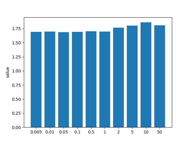
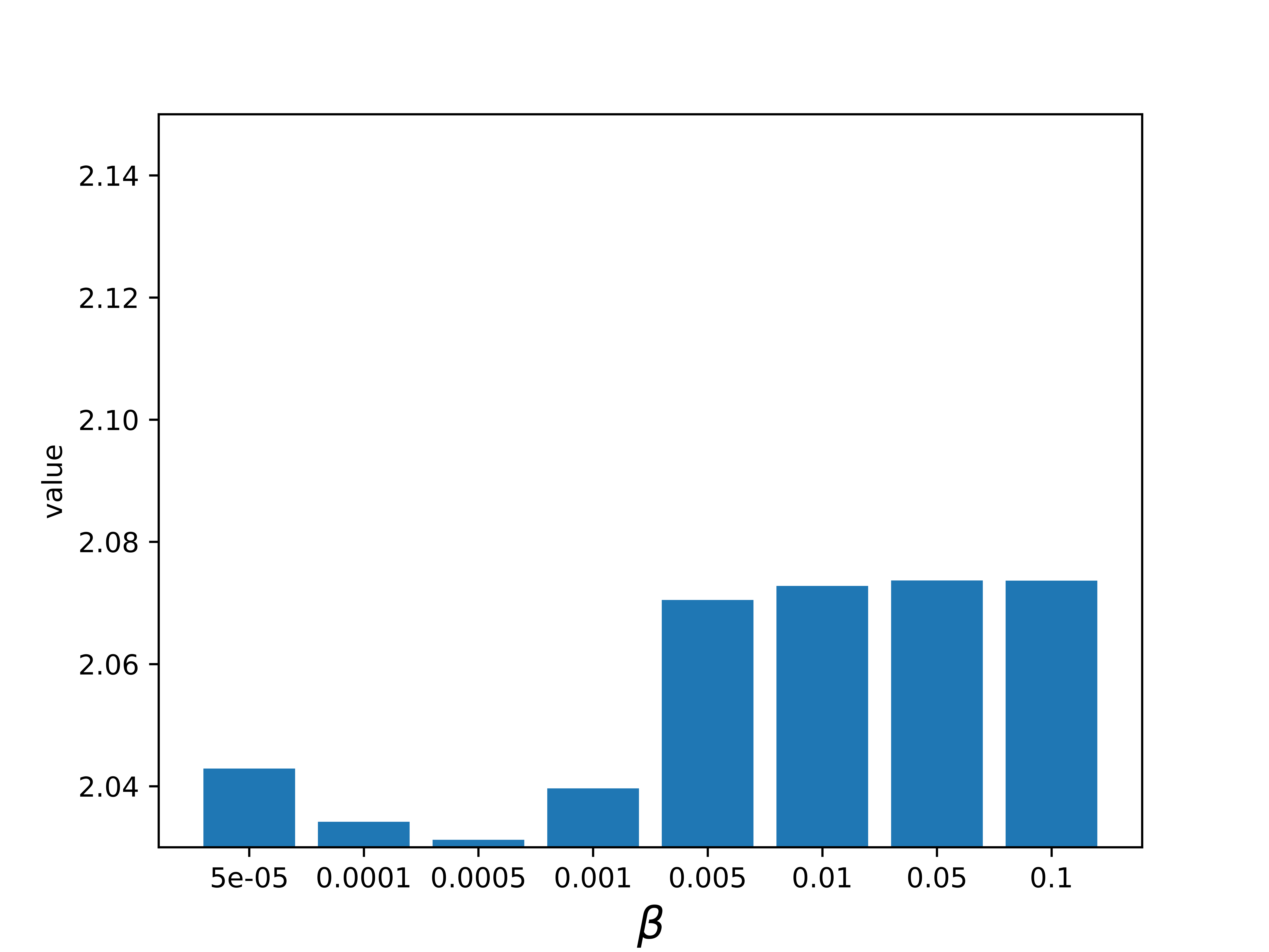
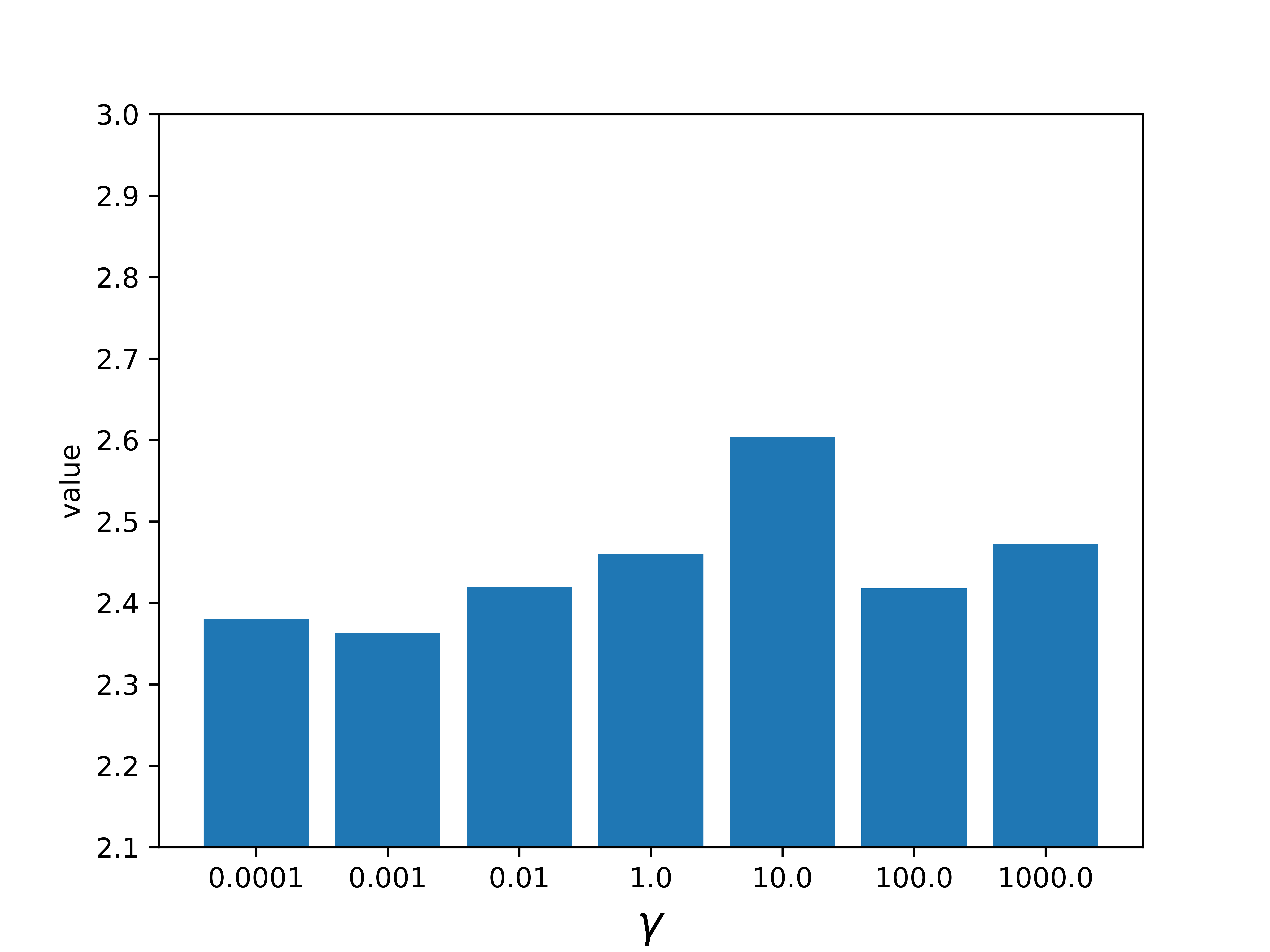
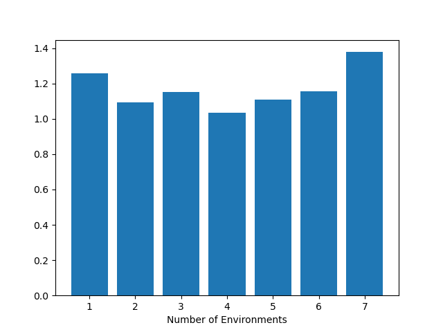
Figure 5: Experiment results of different values of $\alpha,\beta,\gamma$, and prior number of environments

Appendix G Model Efficiency

Following (Liu et al., 2023b) We conduct model efficiency comparasion from three perspectives: forecasting performance, training speed, and memory footprint, which is shown in Figure 6. Compared with other models for nonstationary time-series forecasting, we can find that the proposed IDEA model enjoys the best high model performance and model efficiency, this is because our IDEA is built on MLP-based neural architecture. Compared with other methods like MICN and DLinear, our method achieves a weaker model efficiency, this is because our model needs to model the latent-variable-wise prior.

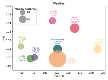
(a) Weather

(b) Exchange

Figure 6: Model efficiency comparison. Training time and memory footprint are recorded with the

Appendix H Implementation Details

We summarize our network architecture below and describe it in detail in Table 6.

Table 6: Architecture details. BS: batch size, T: length of time series, LeakyReLU: Leaky Rectified Linear Unit, $|{\mathbf{x}}_{t}|$: the dimension of ${\mathbf{x}}_{t}$.

Configuration	Description	Output
1. $\psi_{s}$	Stationary Latent Variable Encoder
input:$x_{1:t}$	Observed time series	BS $\times t\times|{\mathbf{x}}_{t}|$
Permute	Matrix Transpose	BS $\times$ $|{\mathbf{x}}_{t}|$ $\times t$
Dense	384 neurons,LeakyReLU	BS $\times$ $n_{s}$ $\times 384$
Dense	t neurons	BS $\times$ $n_{s}$ $\times t$
Permute	Matrix Transpose	BS $\times t$ $\times n_{s}$
2. $T_{s}$	Stationary Latent Variable Prediction Module
Input:$z^{s}_{1:t}$	Stationary Latent Variables	BS $\times t$ $\times n_{s}$
Permute	Matrix Transpose	BS $\times n_{s}$ $\times$ t
Dense	384 neurons,LeakyReLU	BS $\times n_{s}$ $\times$ 384
Dense	T-t neurons	BS $\times n_{s}$ $\times(T-t)$
Permute	Matrix Transpose	BS $\times(T-t)$ $\times n_{s}$
3.$\psi_{e}$	Nonstationary Latent Variable Encoder
input:$x_{1:t}$	Observed time series	Batch Size $\times$ t $\times$ X dimension
Permute	Matrix Transpose	BS $\times|{\mathbf{x}}_{t}|$ $\times t$
Dense	384 neurons,LeakyReLU	BS $\times|{\mathbf{x}}_{t}|$ $\times 384$
Dense	128 neurons	BS $\times|{\mathbf{x}}_{t}|$ $\times 128$
Dense	384 neurons,LeakyReLU	BS $\times n_{e}$ $\times 384$
Dense	t neurons	BS $\times n_{e}$ $\times t$
Permute	Matrix Transpose	BS $\times$ t $\times n_{e}$
4.$T_{e}$	Nonstationary Latent Variable Prediction Module
Input:$z^{e}_{1:t}$	Nonstationary Latent Variables	BS $\times t$ $\times n_{e}$
Permute	Matrix Transpose	BS $\times n_{e}$ $\times t$
Dense	384 neurons,LeakyReLU	BS $\times n_{e}$ $\times 384$
Dense	T-t neurons	BS $\times n_{e}$ $\times(T-t)$
Permute	Matrix Transpose	BS $\times(T-t)$ $\times n_{e}$
5.$F_{x}$	Historical Decoder
Input:$z^{s}_{1:t},z^{e}_{1:t}$	Stationary and nonstationary Latent Variable	BS$\times$ t $\times n_{s}$, BS$\times$ t$\times n_{e}$
Concat	concatenation	BS $\times$ t $\times$ ($n_{e}+n_{s}$)
Dense	x dimension neurons	BS $\times$ t $\times|{\mathbf{x}}_{t}|$
Permute	Matrix Transpose	BS $\times|{\mathbf{x}}_{t}|$ $\times t$
Dense	384 neurons,RelU	BS $\times|{\mathbf{x}}_{t}|$ $\times$ 384
Dense	t neurons	BS $\times|{\mathbf{x}}_{t}|$ $\times t$
Permute	concatenation	BS $\times$ t $\times|{\mathbf{x}}_{t}|$
6.$F_{y}$	Future Predictor
Input:$z^{s}_{t+1:T},z^{e}_{t+1:T}$	Stationary and Nonstationary Latent Variable	BS $\times(T-t)$ $\times n_{s}$ ,BS$\times(T-t)$ $\times n_{e}$
Concat	concatenation	BS $\times(T-t)$ $\times$ ($n_{e}+n_{s}$)
Dense	x dimension neurons	BS $\times(T-t)$ $\times|{\mathbf{x}}_{t}|$
Permute	Matrix Transpose	BS $\times|{\mathbf{x}}_{t}|$ $\times(T-t)$
Dense	384 neurons,LeakyReLU	BS $\times|{\mathbf{x}}_{t}|$ $\times 384$
Dense	T-t neurons	BS $\times|{\mathbf{x}}_{t}|$ $\times(T-t)$
Permute	Matrix Transpose	BS $\times(T-t)$$\times|{\mathbf{x}}_{t}|$
7.$r$	Modular Prior Networks
Input:$z^{s}_{1:T}$ or $z^{e}_{1:T}$	Latent Variables	BS $\times$ $(n_{*}+1)$
Dense	128 neurons,LeakyReLU	$(n_{*}+1)\times 128$
Dense	128 neurons,LeakyReLU	128$\times$128
Dense	128 neurons,LeakyReLU	128$\times$128
Dense	1 neuron	BS $\times$1
JacobianCompute	Compute log ( det (J))	BS

References

• Allman et al. (2009) Allman, E. S., Matias, C., and Rhodes, J. A. Identifiability of parameters in latent structure models with many observed variables. 2009.
• Bai et al. (2018) Bai, S., Kolter, J. Z., and Koltun, V. An empirical evaluation of generic convolutional and recurrent networks for sequence modeling. arXiv preprint arXiv:1803.01271, 2018.
• Bi et al. (2023) Bi, K., Xie, L., Zhang, H., Chen, X., Gu, X., and Tian, Q. Accurate medium-range global weather forecasting with 3d neural networks. Nature, 619(7970):533–538, 2023.
• Box & Pierce (1970) Box, G. E. and Pierce, D. A. Distribution of residual autocorrelations in autoregressive-integrated moving average time series models. Journal of the American statistical Association, 65(332):1509–1526, 1970.
• Cai et al. (2021) Cai, R., Chen, J., Li, Z., Chen, W., Zhang, K., Ye, J., Li, Z., Yang, X., and Zhang, Z. Time series domain adaptation via sparse associative structure alignment. In Proceedings of the AAAI Conference on Artificial Intelligence, volume 35, pp.  6859–6867, 2021.
• Chatfield (2000) Chatfield, C. Time-series forecasting. CRC press, 2000.
• Comon (1994) Comon, P. Independent component analysis, a new concept? Signal processing, 36(3):287–314, 1994.
• Eldele et al. (2023) Eldele, E., Ragab, M., Chen, Z., Wu, M., Kwoh, C.-K., and Li, X. Contrastive domain adaptation for time-series via temporal mixup. IEEE Transactions on Artificial Intelligence, 2023.
• Elliott et al. (2012) Elliott, R. J., Lau, J. W., Miao, H., and Kuen Siu, T. Viterbi-based estimation for markov switching garch model. Applied Mathematical Finance, 19(3):219–231, 2012.
• Fabius & Van Amersfoort (2014) Fabius, O. and Van Amersfoort, J. R. Variational recurrent auto-encoders. arXiv preprint arXiv:1412.6581, 2014.
• Gu et al. (2020) Gu, A., Dao, T., Ermon, S., Rudra, A., and Ré, C. Hippo: Recurrent memory with optimal polynomial projections. Advances in neural information processing systems, 33:1474–1487, 2020.
• Gu et al. (2021a) Gu, A., Goel, K., and Ré, C. Efficiently modeling long sequences with structured state spaces. arXiv preprint arXiv:2111.00396, 2021a.
• Gu et al. (2021b) Gu, A., Johnson, I., Goel, K., Saab, K., Dao, T., Rudra, A., and Ré, C. Combining recurrent, convolutional, and continuous-time models with linear state space layers. Advances in neural information processing systems, 34:572–585, 2021b.
• Gu et al. (2022) Gu, A., Goel, K., Gupta, A., and Ré, C. On the parameterization and initialization of diagonal state space models. Advances in Neural Information Processing Systems, 35:35971–35983, 2022.
• Hälvä & Hyvarinen (2020) Hälvä, H. and Hyvarinen, A. Hidden markov nonlinear ica: Unsupervised learning from nonstationary time series. In Conference on Uncertainty in Artificial Intelligence, pp. 939–948. PMLR, 2020.
• Higgins et al. (2016) Higgins, I., Matthey, L., Pal, A., Burgess, C., Glorot, X., Botvinick, M., Mohamed, S., and Lerchner, A. beta-vae: Learning basic visual concepts with a constrained variational framework. In International conference on learning representations, 2016.
• Hochreiter & Schmidhuber (1997) Hochreiter, S. and Schmidhuber, J. Long short-term memory. Neural computation, 9(8):1735–1780, 1997.
• Hyndman & Athanasopoulos (2018) Hyndman, R. J. and Athanasopoulos, G. Forecasting: principles and practice. OTexts, 2018.
• Hyvärinen (2013) Hyvärinen, A. Independent component analysis: recent advances. Philosophical Transactions of the Royal Society A: Mathematical, Physical and Engineering Sciences, 371(1984):20110534, 2013.
• Hyvarinen & Morioka (2016) Hyvarinen, A. and Morioka, H. Unsupervised feature extraction by time-contrastive learning and nonlinear ica. Advances in neural information processing systems, 29, 2016.
• Hyvarinen & Morioka (2017) Hyvarinen, A. and Morioka, H. Nonlinear ica of temporally dependent stationary sources. In Artificial Intelligence and Statistics, pp.  460–469. PMLR, 2017.
• Hyvärinen & Pajunen (1999) Hyvärinen, A. and Pajunen, P. Nonlinear independent component analysis: Existence and uniqueness results. Neural networks, 12(3):429–439, 1999.
• Hyvarinen et al. (2019) Hyvarinen, A., Sasaki, H., and Turner, R. Nonlinear ica using auxiliary variables and generalized contrastive learning. In The 22nd International Conference on Artificial Intelligence and Statistics, pp.  859–868. PMLR, 2019.
• Hyvärinen et al. (2023) Hyvärinen, A., Khemakhem, I., and Monti, R. Identifiability of latent-variable and structural-equation models: from linear to nonlinear. arXiv preprint arXiv:2302.02672, 2023.
• Jia et al. (2023) Jia, Y., Lin, Y., Hao, X., Lin, Y., Guo, S., and Wan, H. Witran: Water-wave information transmission and recurrent acceleration network for long-range time series forecasting. In Thirty-seventh Conference on Neural Information Processing Systems, 2023.
• Khemakhem et al. (2020a) Khemakhem, I., Kingma, D., Monti, R., and Hyvarinen, A. Variational autoencoders and nonlinear ica: A unifying framework. In International Conference on Artificial Intelligence and Statistics, pp.  2207–2217. PMLR, 2020a.
• Khemakhem et al. (2020b) Khemakhem, I., Monti, R., Kingma, D., and Hyvarinen, A. Ice-beem: Identifiable conditional energy-based deep models based on nonlinear ica. Advances in Neural Information Processing Systems, 33:12768–12778, 2020b.
• Kim et al. (2019) Kim, T., Ahn, S., and Bengio, Y. Variational temporal abstraction. Advances in Neural Information Processing Systems, 32, 2019.
• Kim et al. (2021) Kim, T., Kim, J., Tae, Y., Park, C., Choi, J.-H., and Choo, J. Reversible instance normalization for accurate time-series forecasting against distribution shift. In International Conference on Learning Representations, 2021.
• Kingma & Ba (2014) Kingma, D. P. and Ba, J. Adam: A method for stochastic optimization. arXiv preprint arXiv:1412.6980, 2014.
• Kong et al. (2022) Kong, L., Xie, S., Yao, W., Zheng, Y., Chen, G., Stojanov, P., Akinwande, V., and Zhang, K. Partial disentanglement for domain adaptation. In International Conference on Machine Learning, pp. 11455–11472. PMLR, 2022.
• Kong et al. (2023a) Kong, L., Huang, B., Xie, F., Xing, E., Chi, Y., and Zhang, K. Identification of nonlinear latent hierarchical models. arXiv preprint arXiv:2306.07916, 2023a.
• Kong et al. (2023b) Kong, L., Ma, M. Q., Chen, G., Xing, E. P., Chi, Y., Morency, L.-P., and Zhang, K. Understanding masked autoencoders via hierarchical latent variable models. In Proceedings of the IEEE/CVF Conference on Computer Vision and Pattern Recognition, pp.  7918–7928, 2023b.
• Korda & Mezić (2018) Korda, M. and Mezić, I. Linear predictors for nonlinear dynamical systems: Koopman operator meets model predictive control. Automatica, 93:149–160, 2018.
• Kruskal (1976) Kruskal, J. B. More factors than subjects, tests and treatments: an indeterminacy theorem for canonical decomposition and individual differences scaling. Psychometrika, 41:281–293, 1976.
• Kruskal (1977) Kruskal, J. B. Three-way arrays: rank and uniqueness of trilinear decompositions, with application to arithmetic complexity and statistics. Linear algebra and its applications, 18(2):95–138, 1977.
• Kumar et al. (2017) Kumar, A., Sattigeri, P., and Balakrishnan, A. Variational inference of disentangled latent concepts from unlabeled observations. arXiv preprint arXiv:1711.00848, 2017.
• Lai et al. (2018) Lai, G., Chang, W.-C., Yang, Y., and Liu, H. Modeling long-and short-term temporal patterns with deep neural networks. In The 41st international ACM SIGIR conference on research & development in information retrieval, pp.  95–104, 2018.
• Lee & Lee (1998) Lee, T.-W. and Lee, T.-W. Independent component analysis. Springer, 1998.
• Li et al. (2023a) Li, Z., Cai, R., Chen, G., Sun, B., Hao, Z., and Zhang, K. Subspace identification for multi-source domain adaptation. In Thirty-seventh Conference on Neural Information Processing Systems, 2023a. URL https://openreview.net/forum?id=BACQLWQW8u.
• Li et al. (2023b) Li, Z., Cai, R., Fu, T. Z., Hao, Z., and Zhang, K. Transferable time-series forecasting under causal conditional shift. IEEE Transactions on Pattern Analysis and Machine Intelligence, 2023b.
• Li et al. (2023c) Li, Z., Xu, Z., Cai, R., Yang, Z., Yan, Y., Hao, Z., Chen, G., and Zhang, K. Identifying semantic component for robust molecular property prediction. arXiv preprint arXiv:2311.04837, 2023c.
• Lim & Zohren (2021) Lim, B. and Zohren, S. Time-series forecasting with deep learning: a survey. Philosophical Transactions of the Royal Society A, 379(2194):20200209, 2021.
• Lippe et al. (2022a) Lippe, P., Magliacane, S., Löwe, S., Asano, Y. M., Cohen, T., and Gavves, E. icitris: Causal representation learning for instantaneous temporal effects. arXiv preprint arXiv:2206.06169, 2022a.
• Lippe et al. (2022b) Lippe, P., Magliacane, S., Löwe, S., Asano, Y. M., Cohen, T., and Gavves, S. Citris: Causal identifiability from temporal intervened sequences. In International Conference on Machine Learning, pp. 13557–13603. PMLR, 2022b.
• Liu et al. (2022) Liu, Y., Wu, H., Wang, J., and Long, M. Non-stationary transformers: Exploring the stationarity in time series forecasting. Advances in Neural Information Processing Systems, 35:9881–9893, 2022.
• Liu et al. (2023a) Liu, Y., Hu, T., Zhang, H., Wu, H., Wang, S., Ma, L., and Long, M. itransformer: Inverted transformers are effective for time series forecasting. arXiv preprint arXiv:2310.06625, 2023a.
• Liu et al. (2023b) Liu, Y., Li, C., Wang, J., and Long, M. Koopa: Learning non-stationary time series dynamics with koopman predictors. arXiv preprint arXiv:2305.18803, 2023b.
• Liu et al. (2023c) Liu, Z., Cheng, M., Li, Z., Huang, Z., Liu, Q., Xie, Y., and Chen, E. Adaptive normalization for non-stationary time series forecasting: A temporal slice perspective. In Thirty-seventh Conference on Neural Information Processing Systems, 2023c.
• Locatello et al. (2019a) Locatello, F., Bauer, S., Lucic, M., Raetsch, G., Gelly, S., Schölkopf, B., and Bachem, O. Challenging common assumptions in the unsupervised learning of disentangled representations. In international conference on machine learning, pp. 4114–4124. PMLR, 2019a.
• Locatello et al. (2019b) Locatello, F., Tschannen, M., Bauer, S., Rätsch, G., Schölkopf, B., and Bachem, O. Disentangling factors of variation using few labels. arXiv preprint arXiv:1905.01258, 2019b.
• Makridakis et al. (2020) Makridakis, S., Spiliotis, E., and Assimakopoulos, V. The m4 competition: 100,000 time series and 61 forecasting methods. International Journal of Forecasting, 36(1):54–74, 2020.
• Nie et al. (2022) Nie, Y., Nguyen, N. H., Sinthong, P., and Kalagnanam, J. A time series is worth 64 words: Long-term forecasting with transformers. arXiv preprint arXiv:2211.14730, 2022.
• Oreshkin et al. (2021) Oreshkin, B. N., Carpov, D., Chapados, N., and Bengio, Y. Meta-learning framework with applications to zero-shot time-series forecasting. In Proceedings of the AAAI Conference on Artificial Intelligence, volume 35, pp.  9242–9250, 2021.
• Rangapuram et al. (2018) Rangapuram, S. S., Seeger, M. W., Gasthaus, J., Stella, L., Wang, Y., and Januschowski, T. Deep state space models for time series forecasting. Advances in neural information processing systems, 31, 2018.
• Salinas et al. (2020) Salinas, D., Flunkert, V., Gasthaus, J., and Januschowski, T. Deepar: Probabilistic forecasting with autoregressive recurrent networks. International Journal of Forecasting, 36(3):1181–1191, 2020.
• Salles et al. (2019) Salles, R., Belloze, K., Porto, F., Gonzalez, P. H., and Ogasawara, E. Nonstationary time series transformation methods: An experimental review. Knowledge-Based Systems, 164:274–291, 2019.
• Schölkopf et al. (2021) Schölkopf, B., Locatello, F., Bauer, S., Ke, N. R., Kalchbrenner, N., Goyal, A., and Bengio, Y. Toward causal representation learning. Proceedings of the IEEE, 109(5):612–634, 2021.
• Sezer et al. (2020) Sezer, O. B., Gudelek, M. U., and Ozbayoglu, A. M. Financial time series forecasting with deep learning: A systematic literature review: 2005–2019. Applied soft computing, 90:106181, 2020.
• Smith et al. (2022) Smith, J. T., Warrington, A., and Linderman, S. W. Simplified state space layers for sequence modeling. arXiv preprint arXiv:2208.04933, 2022.
• Song et al. (2023) Song, X., Yao, W., Fan, Y., Dong, X., Chen, G., Niebles, J. C., Xing, E., and Zhang, K. Temporally disentangled representation learning under unknown nonstationarity. In Thirty-seventh Conference on Neural Information Processing Systems, 2023.
• Spantini et al. (2018) Spantini, A., Bigoni, D., and Marzouk, Y. Inference via low-dimensional couplings. The Journal of Machine Learning Research, 19(1):2639–2709, 2018.
• Surana (2020) Surana, A. Koopman operator framework for time series modeling and analysis. Journal of Nonlinear Science, 30:1973–2006, 2020.
• Träuble et al. (2021) Träuble, F., Creager, E., Kilbertus, N., Locatello, F., Dittadi, A., Goyal, A., Schölkopf, B., and Bauer, S. On disentangled representations learned from correlated data. In International Conference on Machine Learning, pp. 10401–10412. PMLR, 2021.
• Virili & Freisleben (2000) Virili, F. and Freisleben, B. Nonstationarity and data preprocessing for neural network predictions of an economic time series. In Proceedings of the IEEE-INNS-ENNS International Joint Conference on Neural Networks. IJCNN 2000. Neural Computing: New Challenges and Perspectives for the New Millennium, volume 5, pp.  129–134. IEEE, 2000.
• Wang et al. (2022) Wang, H., Peng, J., Huang, F., Wang, J., Chen, J., and Xiao, Y. Micn: Multi-scale local and global context modeling for long-term series forecasting. In The Eleventh International Conference on Learning Representations, 2022.
• Wu et al. (2021) Wu, H., Xu, J., Wang, J., and Long, M. Autoformer: Decomposition transformers with auto-correlation for long-term series forecasting. Advances in Neural Information Processing Systems, 34:22419–22430, 2021.
• Wu et al. (2022) Wu, H., Hu, T., Liu, Y., Zhou, H., Wang, J., and Long, M. Timesnet: Temporal 2d-variation modeling for general time series analysis. arXiv preprint arXiv:2210.02186, 2022.
• Wu et al. (2023) Wu, H., Zhou, H., Long, M., and Wang, J. Interpretable weather forecasting for worldwide stations with a unified deep model. Nature Machine Intelligence, pp.  1–10, 2023.
• Xie et al. (2022) Xie, S., Kong, L., Gong, M., and Zhang, K. Multi-domain image generation and translation with identifiability guarantees. In The Eleventh International Conference on Learning Representations, 2022.
• Yan et al. (2023) Yan, H., Kong, L., Gui, L., Chi, Y., Xing, E., He, Y., and Zhang, K. Counterfactual generation with identifiability guarantees. In 37th International Conference on Neural Information Processing Systems, NeurIPS 2023, 2023.
• Yao et al. (2021) Yao, W., Sun, Y., Ho, A., Sun, C., and Zhang, K. Learning temporally causal latent processes from general temporal data. arXiv preprint arXiv:2110.05428, 2021.
• Yao et al. (2022) Yao, W., Chen, G., and Zhang, K. Temporally disentangled representation learning. Advances in Neural Information Processing Systems, 35:26492–26503, 2022.
• Zeng et al. (2023) Zeng, A., Chen, M., Zhang, L., and Xu, Q. Are transformers effective for time series forecasting? In Proceedings of the AAAI conference on artificial intelligence, volume 37, pp.  11121–11128, 2023.
• Zhang (2003) Zhang, G. P. Time series forecasting using a hybrid arima and neural network model. Neurocomputing, 50:159–175, 2003.
• Zhang & Chan (2007) Zhang, K. and Chan, L. Kernel-based nonlinear independent component analysis. In International Conference on Independent Component Analysis and Signal Separation, pp.  301–308. Springer, 2007.
• Zheng et al. (2022) Zheng, Y., Ng, I., and Zhang, K. On the identifiability of nonlinear ica with unconditional priors. In ICLR2022 Workshop on the Elements of Reasoning: Objects, Structure and Causality, 2022.
• Zhou et al. (2021) Zhou, H., Zhang, S., Peng, J., Zhang, S., Li, J., Xiong, H., and Zhang, W. Informer: Beyond efficient transformer for long sequence time-series forecasting. In Proceedings of the AAAI conference on artificial intelligence, volume 35, pp.  11106–11115, 2021.
• Zhu et al. (2020) Zhu, Y., Min, M. R., Kadav, A., and Graf, H. P. S3vae: Self-supervised sequential vae for representation disentanglement and data generation. In Proceedings of the IEEE/CVF Conference on Computer Vision and Pattern Recognition, pp.  6538–6547, 2020.