Surrogate Models for Vibrational Entropy Based on a Spatial Decomposition

Abstract.

The temperature-dependent behavior of defect densities within a crystalline structure is intricately linked to the phenomenon of vibrational entropy. Traditional methods for evaluating vibrational entropy are computationally intensive, limiting their practical utility. Building on [6] we show that total entropy can be decomposed into atomic site contributions and rigorously estimate the locality of site entropy. This analysis suggests that vibrational entropy can be effectively predicted using a surrogate model for site entropy. We employ machine learning to develop such a surrogate models employing the Atomic Cluster Expansion model. We supplement our rigorous analysis with an empirical convergence study. In addition we demonstrate the performance of our method for predicting vibrational formation entropy and attempt frequency of the transition rates, on point defects such as vacancies and interstitials.

1. Introduction

Entropy plays a crucial role in understanding and characterizing the behavior exhibited by condensed matter systems, particularly in the context of crystalline materials undergoing the aging process. The thermodynamic and kinetic characteristics of defects within these materials significantly influence their evolution, resulting in a diverse range of morphologies distinguished by variations in size, character, and density. The role of entropy becomes particularly prominent in indicating how the stability of defect populations changes in response to temperature fluctuations.

Vibrational entropy, arising from the thermal movement of the lattice structure, emerges as a critical component in this context. At temperatures below the melting point, the vibrational aspect takes precedence, becoming the primary contributor to the total entropy. Consequently, assessing vibrational entropy provides valuable insights into the behavior of system in various practical scenarios. However, a fundamental challenge in evaluating harmonic vibrational entropy lies in the computational costs. The classical approach involves calculating the dynamical matrix, a process requiring on the order of $O(N^{2})$ calculations, and subsequent diagonalization, which demands $O(N^{3})$ calculations, with $N$ representing the total number of atoms in the system. As a result, the computation of entropy on large length scales becomes computationally intractable, presenting a computational challenge that needs to be addressed.

To overcome this computational challenge, recent work by Lapointe et al. [30] has employed machine learning surrogate models utilizing atomic environment descriptors. These models offer precise predictions for the vibrational formation entropy of point defects, achieving significant computational efficiency with calculations on the order of $O(N)$. The versatility of these data-driven models is further enhanced by the incorporation of higher-dimensional descriptor spaces, establishing a non-linear relationship between descriptors and observables [31]. This advancement enables a more comprehensive representation of physical phenomena, such as defect formation and migration, essential for accurate rate approximations in transition state theory. However, it is noteworthy that these studies implicitly assumed that the total vibrational entropy can be expressed as a local contribution, and the resulting site entropy is local. Limited research has delved into a rigorous analysis of vibrational entropy. To the best knowledge of the authors, the only existing work in this domain is [6]. In this study, the formation free energy and transition rates between stable configurations, assessed using periodic supercell approximations, converge as the cell size increases. While this work implicitly utilized the locality of site entropy, it cannot be directly applied to justify machine learning surrogates.

The purpose of the present paper is to undertake a rigorous analysis of the locality of site entropy, utilizing insights presented from [6], where total entropy was deconstructed into contributions from individual atomic sites. This analysis establishes the groundwork for constructing entropy based on the local atomic environment. Building upon this foundation, we employ machine learning surrogate models with atomic environment descriptors to precisely and efficiently predict the vibrational formation entropy of crystalline defects. To that end we utilize the Atomic Cluster Expansion (ACE) method, widely applied in the field of machine-learning interatomic potentials (MLIPs) for atomistic simulations. Numerical experiments are conducted, focusing on point defects such as vacancies and interstitials. The robustness of our approach is demonstrated by accurately predicting vibrational entropy and the attempt frequency for the transition rates governing point defect migration, a critical element in transition state theory rate approximations. These results lay the groundwork for predicting various entropy-dependent physical quantities, including but not limited to dynamical properties like free energy and diffusion coefficients, which can potentially be integrated into kinetic Monte Carlo methods [43], where transition rates from state to state are pivotal.

This paper primarily concentrates on relatively simple settings (point defects) to provide a comprehensive theoretical and practical analysis of key concepts, but a wide variety of extensions to more complex classes of crystalline defects, and to other classes of materials are conceivable.

Outline

In Section 2, we establish the foundation for our theories by offering background information and preliminaries. This includes rigorous derivations of both total and site entropy. Section 3 presents our primary findings (Theroem 3.1), focusing on the locality of site entropies in an infinite lattice $\Lambda$, supported by numerical results validating our main theorem. Moving on to Section 4, we delve into the background of the surrogate models utilized for entropy fitting and subsequently present our entropy and corresponding attempt frequency fitting results. The Appendices contain a compilation of auxiliary results and proofs essential for the understanding and validation of the preceding sections.

Notation

Let $X$ be a (semi-)Hilbert space and let its dual be represented by $X^{*}$. The duality pairing is denoted by $\langle\cdot,\cdot\rangle$. The space of bounded linear operators mapping from $X$ to another (semi-)Hilbert space $Y$ is expressed as $\mathcal{L}(X,Y)$.

For $\mathcal{E}\in C^{2}(X)$, the first and second variations are denoted by $\langle\delta\mathcal{E}(u),v\rangle$ and $\langle\delta^{2}\mathcal{E}(u)v,w\rangle$ for $u,v,w\in X$, i.e.,

$$\langle\delta\mathcal{E}(u),v\rangle :=\lim_{t\rightarrow 0}t^{-1}\big{(}\mathcal{E}(u+tv)-\mathcal{E}(u)\big{)},$$

$$\langle\delta^{2}\mathcal{E}(u)v,w\rangle :=\lim_{t\rightarrow 0}t^{-2}\langle\delta\mathcal{E}(u+tw)-\delta\mathcal{E}(u),v\rangle.$$

It is easy to see that $\delta\mathcal{E}(x)\in X^{*}$ and $\delta^{2}\mathcal{E}(x)\in\mathcal{L}(X,X^{*})$.

Assuming $\Lambda$ is a countable index set (often a Bravais lattice, $\Lambda={\sf A}\mathbb{Z}^{d}$, with ${\sf A}\in\mathbb{R}^{d\times d}$ being non-singular), we define $\ell^{2}(\Lambda;\mathbb{R}^{m})=\{u:\Lambda\to\mathbb{R}^{m}:\sum_{\ell\in\Lambda}|u|^{2}<\infty\}$. If the range is evident from the context, this can be abbreviated to $\ell^{2}(\Lambda)$ or simply $\ell^{2}$.

For $A\in\mathcal{L}\big{(}\ell^{2}(\Lambda;\mathbb{R}^{m}),\ell^{2}(\Lambda;\mathbb{R}^{m})\big{)}$, we define its element $A_{\ell inj}:=\big{\langle}A(\delta_{\ell}e_{i}),\delta_{n}e_{j}\big{\rangle}_{\ell^{2}(\Lambda;\mathbb{R}^{d})}$, where $\ell,n\in\Lambda$ and $i,j\in\{1,\ldots,m\}$. Additionally, we denote $A_{\ell n}=(A_{\ell inj})_{ij}\in\mathbb{R}^{m\times m}$ as the matrix blocks corresponding to atomic sites. The identity is represented by $(I_{\ell^{2}(\Lambda;\mathbb{R}^{m})})_{\ell inj}:=\delta_{\ell n}\delta_{ij}$.

For $j\in\mathbb{N}$, ${\bm{g}}\in(\mathbb{R}^{d})^{A}$, and $V\in C^{j}\big{(}(\mathbb{R}^{d})^{A}\big{)}$, we define the notation

$$V_{,{\bm{\rho}}}\big{(}{\bm{g}}\big{)}:=\frac{\partial^{j}V\big{(}{\bm{g}}\big{)}}{\partial{\bm{g}}_{\rho_{1}}\cdots\partial{\bm{g}}_{\rho_{j}}}\qquad{\rm for}\quad{\bm{\rho}}=(\rho_{1},\ldots,\rho_{j})\in A^{j}.$$

The symbols $C,c$ denote generic positive constants that may change from one line of an estimate to the next. When estimating rates of decay or convergence, $C,c$ will always remain independent of approximation parameters such as the system size, the configuration of the lattice and the test functions. The dependence of $C,c$ will be clear from the context or stated explicitly. To further simplify notation we will often write $\lesssim$ to mean $\leq C$.

2. Background and Preliminaries

Although our approach to constructing surrogates for vibration entropy is very general, our rigorous analysis relies on the setting of crystalline solids, potentially with defects. To motivate the formulation of our main results in this context, we will review the framework developed in [7, 13, 35] and in particular the renormalisation analysis of vibrational formation entropy [6]. For the sake of simplicity of presentation, we will skip over some technical details but fill these gaps in Appendix A.1.

Let $d\in\{2,3\}$ be the dimension of the system. A homogeneous crystal reference configuration is given by the Bravais lattice $\Lambda^{\rm hom}=\mathsf{A}\mathbb{Z}^{d}$, for some non-singular matrix $\mathsf{A}\in\mathbb{R}^{d\times d}$. We admit only single-species Bravais lattices. There are no conceptual obstacles to generalising our work to multi-lattices [34], however, the technical details become more involved. The reference configuration with defects is a set $\Lambda\subset\mathbb{R}^{d}$. The mismatch between $\Lambda$ and $\Lambda^{\rm hom}$ represents possible defected configurations. We assume that the defect cores are localized, that is, there exists $R^{\rm def}>0$, such that $\Lambda\backslash B_{R^{\rm def}}=\Lambda^{\rm hom}\backslash B_{R^{\rm def}}$.

The displacement of the infinite lattice $\Lambda$ is a map $u\colon\Lambda\to\mathbb{R}^{m}$. For $\ell,\rho\in\Lambda$, we denote discrete gradients (or, differences) by $D_{\rho}u(\ell):=u(\ell+\rho)-u(\ell)$. Higher order differences are denoted by $D_{\bm{\rho}}=D_{\rho_{1}}\cdots D_{\rho_{j}}$ for a $\bm{\rho}=(\rho_{1},...,\rho_{j})\in\Lambda^{j}$. For a subset $\mathcal{R}\subset\Lambda-\ell$, we define $Du(\ell):=D_{\mathcal{R}_{\ell}}u(\ell):=\big{(}D_{\rho}u(\ell)\big{)}_{\rho\in\mathcal{R}_{\ell}}$. We assume throughout that $\mathcal{R}_{\ell}$ is finite for each site $\ell\in\Lambda$. An extension of our analysis to infinite interaction range is not conceptually difficult but involves additional technical and notational complexities [10].

We consider the site potential to be a collection of mappings $V_{\ell}:(\mathbb{R}^{m})^{\mathcal{R}_{\ell}}\rightarrow\mathbb{R}$, which represent the energy distributed to each atomic site. We make the following assumption on regularity and symmetry: $V_{\ell}\in C^{K}\big{(}(\mathbb{R}^{m})^{\mathcal{R}_{\ell}}\big{)}$ for some $K$ and $V_{\ell}$ is homogeneous outside the defect region, namely, $V_{\ell}=V$ and $\mathcal{R}_{\ell}=\mathcal{R}$ for $\ell\in\Lambda\setminus B_{R^{\rm def}}$. Furthermore, $V$ and $\mathcal{R}$ have the following point symmetry: $\mathcal{R}=-\mathcal{R}$, it spans the lattice $\textrm{span}_{\mathbb{Z}}\mathcal{R}=\Lambda$, and $V\big{(}\{-A_{-\rho}\}_{\rho\in\mathcal{R}}\big{)}=V(A)$. We refer to [10, Section 2.3] for a detailed discussion of those assumptions.

2.1. Supercell model

Following [6] we initially consider the periodic setting and then reference the established existence of the thermodynamic limit and proceed to analyze the infinite lattice. To that end, let $\mathsf{B}=(b_{1},\ldots,b_{d})\in\mathbb{R}^{d\times d}$ be invertible such that $b_{i}\in\mathsf{A}\mathbb{Z}^{d}$. For a sufficiently large $N\in\mathbb{N}$ with $R^{\rm def}\ll N$, we denote

$$\Lambda_{N}:=\Lambda\cap\mathsf{B}(-N/2,N/2]^{d}\quad\textrm{and}\quad\Lambda_{N}^{{\rm per}}:=\bigcup_{\alpha\in N\mathbb{Z}^{d}}(\mathsf{B}\alpha+\Lambda_{N}),$$

where $\Lambda_{N}$ is the periodic computational domain and $\Lambda_{N}^{{\rm per}}$ is the periodically repeated domain.

We define the space of periodic displacements to be

$$\mathcal{W}^{\text{per}}_{N}:=\{u:\Lambda_{N}^{{\rm per}}\rightarrow\mathbb{R}^{m}~{}|~{}u(\ell+\mathsf{B}\alpha)=u(\ell)~{}\textrm{for}~{}\alpha\in N\mathbb{Z}^{d}\}.$$

An equilibrium defect geometry configuration is determined by

$$\bar{u}_{N} \in\arg\min\{\mathcal{E}_{N}(u)~{}|~{}u\in\mathcal{W}^{\text{per}}_{N}\},$$

$$\text{where}~{}\mathcal{E}_{N} (u):=\sum_{\ell\in\Lambda_{N}}V_{\ell}\big{(}Du(\ell)\big{)}\quad\text{for}~{}u\in\mathcal{W}^{\text{per}}_{N}.$$ (2.1)

Analogously, for future reference, we introduce the energy functional for the homogeneous (defect-free) supercell as

$$\mathcal{E}^{\text{hom}}_{N}(u):=\sum_{\ell\in\Lambda_{N}}V\big{(}Du(\ell)\big{)}\quad\text{ for }u\in\mathcal{W}^{\text{per}}_{N}.$$ (2.2)

2.2. Vibrational entropy

The vibrational entropy is closely related to the formation free energy. This is used in, for example, phase diagrams [19], diffusion coefficients [17], equilibrium concentration of defects [42].

In the harmonic approximation model (thus incorporating only vibrational entropy into the model) we approximate a nonlinear potential energy landscape (cf. (2.1) and (2.2)) by a quadratic expansion about an energy minimizer of interest,

$$\mathcal{E}^{\rm hom}_{N}(w) \approx{\textstyle\frac{1}{2}}\langle H^{\rm hom}_{N}w,w\rangle,\quad\text{and}$$ (2.3)

$$\mathcal{E}_{N}(\bar{u}_{N}+w) \approx\mathcal{E}_{N}(\bar{u}_{N})+{\textstyle\frac{1}{2}}\langle H_{N}(\bar{u}_{N})w,w\rangle,$$ (2.4)

where we use the fact that $\delta\mathcal{E}^{{\rm hom}}_{N}({\bf 0})$ and $\delta\mathcal{E}_{N}(\bar{u}_{N})$ vanish. Additionally, we denote $H_{N}(u):=\delta^{2}\mathcal{E}_{N}(u),\;H^{\text{hom}}_{N}(u):=\delta^{2}\mathcal{E}^{\text{hom}}_{N}(u),$ and $H^{\text{hom}}_{N}:=H^{\text{hom}}_{N}({\bf 0})$ for the Hessians of systems.

The free energy of a system is intimately tied to the partition function. The harmonic approximation of the partition function is given by

$$Z_{\rm h} =e^{-\beta\mathcal{E}_{N}(\bar{u}_{N})}\int e^{-\beta\frac{1}{2}\langle H_{N}(\bar{u}_{N})w,w\rangle}\mathrm{d}w$$ (2.5)

$$=C_{\beta,N}\cdot e^{-\beta\mathcal{E}_{N}(\bar{u}_{N})}\cdot\big{(}\text{det}^{+}(H_{N})\big{)}^{-1/2},$$

where the constant $C_{\beta,N}=(2\pi/\beta)^{((2N)^{d}-1)m/2}$ with $\beta:=1/k_{B}T$ the inverse temperature. Here $\det^{+}(H_{N}):=\prod_{j}\lambda_{j}$ with $\lambda_{j}$ representing the positive eigenvalues of $H_{N}$ including multiplicities [6]. The harmonic approximation to the partition function for the homogeneous system can be analogously defined by

$$Z_{\rm h}^{\text{hom}}=C_{\beta,N}\cdot\big{(}\text{det}^{+}(H^{\text{hom}}_{N})\big{)}^{-1/2}.$$ (2.6)

Hence, the harmonic approximation of the Helmholtz formation free energy is defined by

$$\mathcal{A}(\bar{u}_{N}) :=-\frac{1}{\beta}\log\left(\frac{Z_{\rm h}}{Z_{\rm h}^{\text{hom}}}\right)$$ (2.7)

$$=\mathcal{E}_{N}(\bar{u}_{N})-k_{B}T\Big{(}-\frac{1}{2}\log\text{det}^{+}\big{(}H_{N}(\bar{u}_{N})\big{)}+\frac{1}{2}\log\text{det}^{+}\big{(}H^{\text{hom}}_{N}\big{)}\Big{)}$$

$$=\mathcal{E}_{N}(\bar{u}_{N})-T\mathcal{S}_{N}(\bar{u}_{N}),$$

where the vibrational formation entropy is

$$\mathcal{S}_{N}(\bar{u}_{N}):=\frac{k_{B}}{2}\Big{(}\log\text{det}^{+}\big{(}H^{\text{hom}}_{N}\big{)}-\log\text{det}^{+}\big{(}H_{N}(\bar{u}_{N})\big{)}\Big{)}.$$ (2.8)

In solid state physics, it is common to employ the density of states (DOS) as the basis for defining entropy. In Appendix B, we show that this perspective yields the same entropy as (2.7).

An important material property related to the vibrational entropy is the transition rate (e.g., in the context of defect motion via diffusion). We will explore this in Section 4.4 how our techniques can also be applied in that setting.

2.3. Site entropy

For systems with a large number of atoms, the computational expense associated with evaluating vibrational entropy via the eigendecomposition, or Cholesky factorisation, of the hessian matrix is prohibitive. The objective of this work is to develop a surrogate model for vibrational entropy with linear scaling cost. The key step towards that end is a spatial decomposition into local site entropy contributions. We adopt the spatial decomposition proposed in [6], which is closely related to the one used for defining site energies in the tight-binding model [11].

To establish the aforementioned spatial decomposition, we employ a self-adjoint operator $\textbf{F}_{N}:\mathcal{W}^{\text{per}}_{N}\rightarrow\mathcal{W}^{\text{per}}_{N}$ which acts as $(H^{\text{hom}}_{N})^{-1/2}$. The existence and properties of $\textbf{F}_{N}$ has been previously established in [6, Lemma 2.5].

We first rewrite the entropy difference (2.7) as

$$\mathcal{S}_{N}(u)=-\frac{1}{2}\operatorname{Trace}\,\log^{+}{(\textbf{F}_{N}H_{N}(u)\textbf{F}_{N})},$$ (2.9)

where $\log^{+}$ is defined as follows:

Figure 1. Depiction of the spectrum of $\mathbf{T}$, where $\sigma(\mathbf{T})\cap(0,\infty)\subset[m,M]$ along with the appropriate contour $\mathcal{C}$.

Let $\mathbf{T}$ be a bounded, self-adjoint operator on a Hilbert space with spectrum $\sigma(\mathbf{T})\subset(-\infty,0]\cup[m,M]$ where $0<m\leq M$, as depicted in Figure 1. Then, we can define a contour $\mathcal{C}$ that encircles the interval $[m,M]$ but remains in the right half-plane. Using resolvent calculus we can now define (cf. [6] for more details)

$$\log^{+}\mathbf{T}=\frac{1}{2\pi i}\oint_{\mathcal{C}}\log(z)\cdot(z\mathbf{I}-\mathbf{T})^{-1}\,{\rm d}z.$$ (2.10)

The trace operation in (2.9) is interpreted as a spatial decomposition from [6], allowing us to write

$$\mathcal{S}_{N}(u) =\sum_{\ell\in\Lambda_{N}}\mathcal{S}_{N,\ell}(u),\qquad\text{where}$$ (2.11)

$$\mathcal{S}_{N,\ell}(u) :=-\frac{1}{2}\operatorname{Trace}\big{[}\log^{+}(\textbf{F}_{N}H_{N}(u)\textbf{F}_{N})\big{]}_{\ell\ell},$$ (2.12)

where $[L]_{\ell\ell}$ denotes the $3\times 3$ block of $L$ corresponding to an atomic site $\ell\in\Lambda$. The site entropy $\mathcal{S}_{N,\ell}$ will be our central object of study.

2.4. Thermodynamic limit

While our computational investigations will be for the supercell model, the analysis is more convenient to perform in infinite lattice limit. We therefore review relevant results from [6, 8, 14].

We now consider displacement fields that are either compactly supported or of finite energy, characterized by the function spaces

$$\dot{\mathcal{W}}^{\rm c} :=\left\{u:\Lambda\rightarrow\mathbb{R}^{m}\mid\text{supp}(Du)\text{ is compact}\right\},\quad\text{and}$$

$$\dot{\mathcal{W}}^{1,2} :=\left\{u:\Lambda\rightarrow\mathbb{R}^{m}\mid\|Du\|_{\ell^{2}}<\infty\right\},$$

where

$$|Du(\ell)|^{2}=\sum_{\rho\in R_{\ell}}|D_{\rho}u(\ell)|^{2},\qquad\|Du\|_{\ell^{2}(\Lambda)}=\left(\sum_{\ell\in\Lambda}|Du(\ell)|^{2}\right)^{1/2}.$$ (2.13)

The above expressions define a semi-norm for both $\dot{\mathcal{W}}^{c}$ and $\dot{\mathcal{W}}^{1,2}$ spaces. The energy functionals for the homogeneous and defective lattice are defined respectively as

$$\mathcal{E}_{\text{hom}}(u) =\sum_{\ell\in\Lambda}V\big{(}Du(\ell)\big{)},$$ (2.14)

$$\mathcal{E}(u) =\sum_{\ell\in\Lambda}V_{\ell}\big{(}Du(\ell)\big{)}\quad\text{for }u\in\dot{\mathcal{W}}^{c}.$$ (2.15)

We now consider the equilibrium configurations, $\delta\mathcal{E}(\bar{u})=0$ which can equivalently be written as

$$\langle\delta\mathcal{E}(\bar{u}),v\rangle=0.$$ (2.16)

Theorem 2.1 (Thermodynamic Limit). [8, Theorem 2.1] Let $\bar{u}\in\dot{\mathcal{W}}^{1,2}$ be a stable solution to (2.16). For $N$ sufficiently large, there exists a locally unique solution to (2.1) such that the following estimates hold:

$$\|D\bar{u}_{N}-D\bar{u}\|_{\ell^{\infty}(\Lambda_{N})} \leq CN^{-d},$$ (2.17)

$$\|D\bar{u}_{N}-D\bar{u}\|_{\ell^{2}(\Lambda_{N})} \leq N^{-d/2},$$ (2.18)

$$|\mathcal{E}_{N}(\bar{u}_{N})-\mathcal{E}(\bar{u})| \leq N^{-d}.$$ (2.19)

Furthermore, the thermodynamic limit of $\mathcal{S}_{N}$ as $N\to\infty$, denoted by $\mathcal{S}$, exists. The error in approximating $\mathcal{S}(\bar{u})$ with $\mathcal{S}_{N}(\bar{u}_{N})$ satisfies [6, Theorem 2.3]

$$\left|\mathcal{S}(\bar{u})-\mathcal{S}_{N}(\bar{u}_{N})\right|\lesssim N^{-d}\log^{5}(N).$$ (2.20)

Additionally, in [6, Lemma 3.2], it is shown that there exist $\underline{\sigma},\bar{\sigma},\varepsilon>0$ and a contour $\mathcal{C}$ encircling $[\underline{\sigma},\bar{\sigma}]$ but not the origin, such that, if some $u_{\infty}\in\dot{\mathcal{W}}^{1,2}$ satisfies $\sigma\big{(}{\rm\textbf{F}}^{*}H(u_{\infty})\textbf{F}\big{)}\cap(-\underline{\sigma},\infty)\subset[2\underline{\sigma},\overline{\sigma}/2]$ for some $0<\underline{\sigma}<\overline{\sigma}$, then for all $u\in B_{\varepsilon}(u_{\infty})$, the operator $\boldsymbol{\rm F}^{*}H(u)\boldsymbol{\rm F}$ remains uniformly bounded above and below and

$$\log^{+}\big{[}{\rm\textbf{F}}^{*}H(u)\textbf{F}\big{]}= ~{}\frac{1}{2\pi i}\oint_{\mathcal{C}}\log(z)\cdot\mathscr{R}_{z}(u)\,{\rm d}z,$$

$$\textrm{where}~{}\mathscr{R}_{z}=\mathscr{R}_{z}(u):= ~{}(zI-\boldsymbol{\rm F}^{*}H(u)\boldsymbol{\rm F})^{-1}.$$ (2.21)

From now on, we will fix this contour and always have $z\in\mathcal{C}$. We will also express the limit quantity for each site entropy $S_{N,\ell}$ using the generalized notation

$$\mathcal{S}_{\ell}(u):=-\frac{1}{2}\operatorname{Trace}\big{[}\log^{+}(\textbf{F}^{*}H(u)\textbf{F})\big{]}_{\ell\ell}\quad\textrm{with}\quad\textbf{F}:=(H^{\text{hom}})^{-1/2}\in\mathcal{L}(\ell^{2},\dot{\mathcal{W}}^{1,2})$$ (2.22)

where $(H^{\text{hom}})^{-1/2}$ denotes the square root of the pseudo-inverse of $H^{\text{hom}}$. For a more detailed discussion on the existence of F and a rigorous definition using Fourier transform see Appendix A.1.

The homogeneous site entropy can be similarly defined by

$$\mathcal{S}^{\text{hom}}_{\ell}(u):=-\frac{1}{2}\operatorname{Trace}\big{[}\log^{+}(\textbf{F}^{*}H^{\text{hom}}(u)\textbf{F})\big{]}_{\ell\ell}.$$ (2.23)

Following the arguments in the proof of [6, Proposition 5.8], the existence of a similar limit quantity for $\mathcal{S}_{N,\ell}(\bar{u}_{N})$, namely $\mathcal{S}_{\ell}(\bar{u})$ can be deduced. Thus, instead of analyzing the supercell approximation of site entropy $\mathcal{S}_{N,\ell}(u)$, we will give a locality estimate of $\mathcal{S}_{\ell}(u)$ (cf. Theorem 3.1) in the subsequent section.

3. Locality of Site Entropy

We begin by thoroughly analyzing the locality of site entropy, establishing a foundation for its subsequent impact on the error analysis arising from the truncation of the interaction range in Section 3.1. To substantiate our theoretical results, a numerical validation of the locality estimate is presented in Section 3.2.

3.1. Locality Estimates for $\mathcal{S}_{\ell}$

It is shown in [6] that each individual entropy $\mathcal{S}_{\ell}$ has only a small dependence on distant atomic sites. A concrete representation of this decay is provided by the formal estimate

$$\left|\frac{\partial\mathcal{S}_{\ell}(\bar{u})}{\partial Du_{n}}-\frac{\partial\mathcal{S}^{\text{hom}}_{\ell}({\bf 0})}{\partial Du_{n}}\right|\lesssim|\ell-n|^{-2d}|n|^{-d}+\text{higher order terms}.$$ (3.1)

This equation provides an initial glimpse into the localized characteristics of $\mathcal{S}_{\ell}$ and sheds light on why one might anticipate effective control over its summation across $\ell$. A more precise estimate for this locality will be established in the remainder of the section, building on the machinery developed in [6]. Our goal in this section is to show that site entropies have a locality property.

Theorem 3.1. (Locality) Given $u\in\dot{\mathcal{W}}^{1,2}$, let the site entropy $\mathcal{S}_{\ell}(u)$ be defined by (2.22). Then there exist a constant $C_{2}>0$ such that, for $\ell,n\in\Lambda$, and for $r_{n\ell}$ sufficiently large,

$$\left|\frac{\partial\mathcal{S}_{\ell}(u)}{\partial u_{n}}\right|\leq C_{2}\big{|}r_{n\ell}\big{|}^{-2d},$$ (3.2)

where $r_{n\ell}$ represents the distance between atoms $n$ and $\ell$.

Theorem 3.1 reveals the locality principle of site entropy, which indicates that the sensitivity of site entropy to displacements decreases algebraically as the distance $r_{n\ell}$ grows. We will numerically validate this theorem in Section 3.2. Owing to this locality, the accurate approximations of $\mathcal{S}^{+}_{\ell}(u)$ can be achieved by limiting the group of atoms with index $j$ to a certain vicinity around atom $\ell$, i.e., $r_{\ell j}<r_{\text{cut}}$. More precisely, given the site $\ell\in\Lambda$, we define the truncated site entropy $\widetilde{\mathcal{S}}^{+}_{\ell}(u)$ by

$$\tilde{\mathcal{S}}_{\ell}(u)=\mathcal{S}_{\ell}(T_{r_{\rm cut}}u)\quad\text{where}\quad T_{r_{\rm cut}}u(k):=\begin{cases}u_{k}&\text{for }k\in\Lambda\cap B_{r_{\rm cut}}(\ell)\\ \boldsymbol{0}&\text{otherwise}\end{cases}.$$ (3.3)

The subsequent theorem suggests that the truncated site entropy $\widetilde{\mathcal{S}}_{\ell}$ defined in (3.3), serves as a reliable approximation to the non-truncated entropy $\mathcal{S}_{\ell}$. We give the complete proof of this theorem in the Appendix A and will be numerically verified in Section 4.3.

Theorem 3.2. Let $\widetilde{\mathcal{S}}_{\ell}({u};r_{\rm cut})$ defined by (3.3) for $u\in\dot{\mathcal{W}}^{1,2}$, denote the truncated site entropy for atomic site $\ell$. Then there exists a constant $C_{3}>0$ such that for $r_{\rm cut}$ sufficiently large,

$$\big{|}\mathcal{S}_{\ell}(u)-\widetilde{\mathcal{S}}_{\ell}(u;r_{\rm cut})\big{|}\leq C_{3}|r_{\rm cut}|^{-d}\cdot\|u\|_{L^{\infty}}.$$ (3.4)

The two foregoing theorems justify calling (2.11) a spatial decomposition. It further motivates developing a surrogate model for vibrational entropy in terms of a sum of parameterized site entropy contributions. We will explore this further in Section 4. In the recent study [31] the spatial localization of site entropy was postulated as an assumption to construct surrogate models for entropy.

3.2. Numerical validation

To validate the locality of site entropy (cf. Theorem 3.1), we consider a toy model with pairwise interactions [20, 45]. We consider lattice displacements as functions $u:\Lambda\to\mathbb{R}$ and define the energy as:

$$E(C;u)=\sum_{i}\left(\sum_{j\in\mathcal{N}_{i}}C_{ij}|u_{i}-u_{j}|^{2}+\delta|u_{i}-u_{j}|^{3}+|u_{i}-u_{j}|^{4}\right),$$ (3.5)

where $i$ indexes the lattice points, $\mathcal{N}_{i}$ denotes the set of nearest neighbors of the $i$-th site, $u_{i}$ represents the displacement at the $i$-th lattice site, $C_{ij}$ are the coefficients characterizing the interactions between points $i$ and $j$, and $\delta$ is a constant which controls the contribution of the strength of the cubic term. (Qualitatively, this is not a severe restriction of generality, see e.g. [6, Section 6.2]).

This form encapsulates the 1D, 2D cases with appropriate definitions of $\mathcal{N}_{i}$ for each dimension. When defining the matrices $C$, we only consider nearest neighbour interactions and employed periodic boundary conditions. Bonds are indicated by the interaction coefficient values, with 1 signifying a bond and 0 its absence. To incorporate inhomogenity into our numerical tests, we integrated “impurities” into the model by introducing perturbations to the existing elements of the matrix $C$. The inclusion of defects and impurities in the system does not impact the locality property of site entropy.

It is noteworthy that the employment of the toy model here instead of real systems, enables us to easily perform large-scale simulation in which we can most clearly observe the anticipated locality behavior.

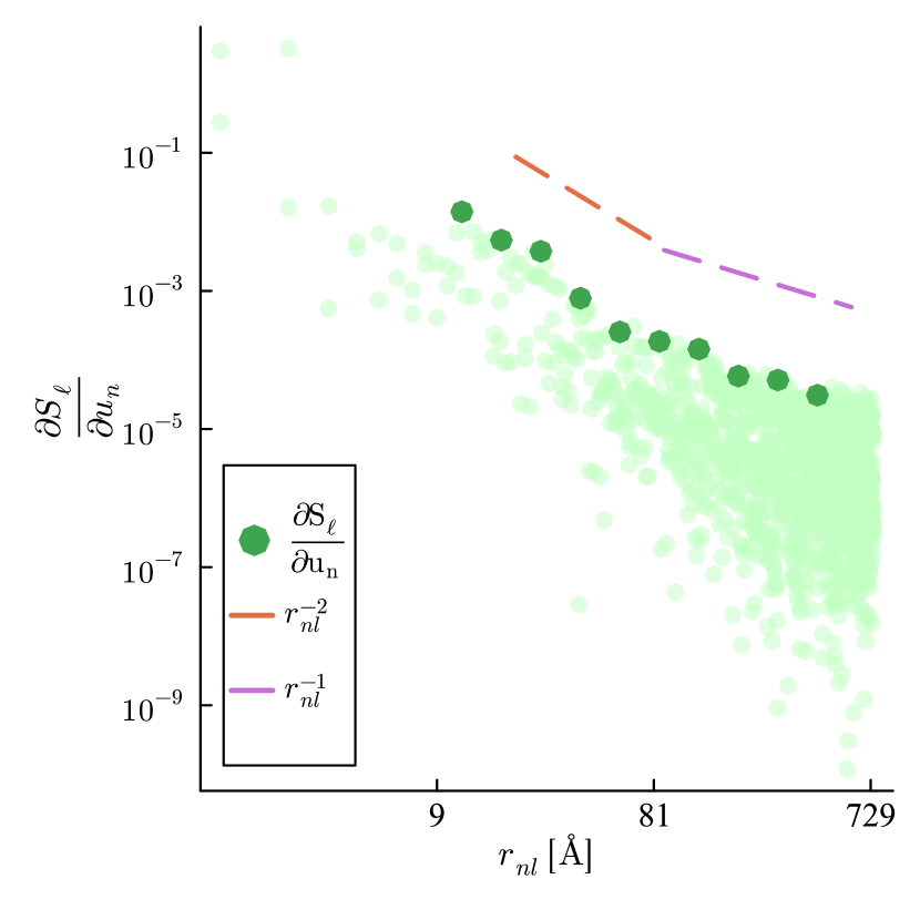
(a) $\delta=0$

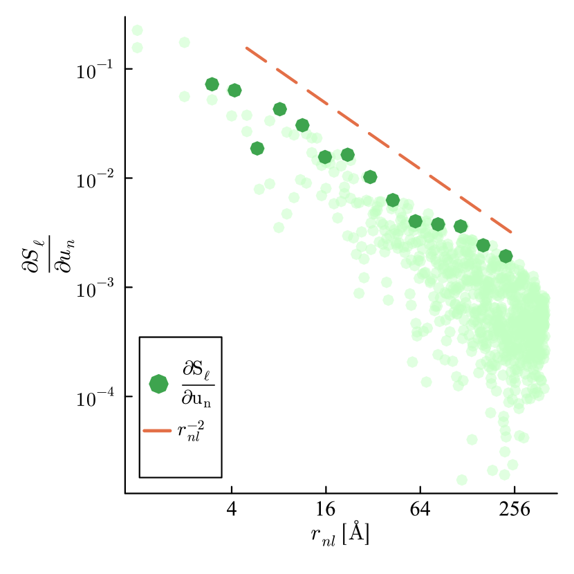
(b) $\delta=0.1$

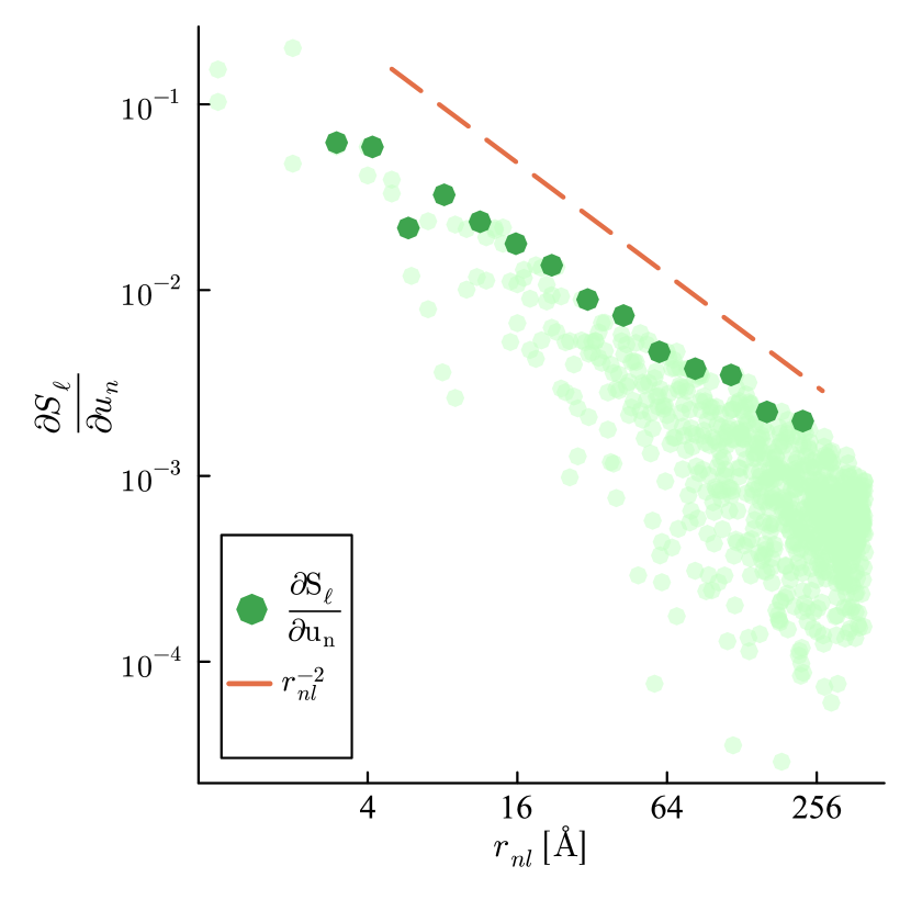
(c) $\delta=0.5$

Figure 2. Derivatives of site entropy for the 1 dimensional toy model including 800 atoms. The dark green dots represent the maximum $\frac{\partial S}{\partial u_{n}}$ values within specified logarithmic bins along the $x$ axis.

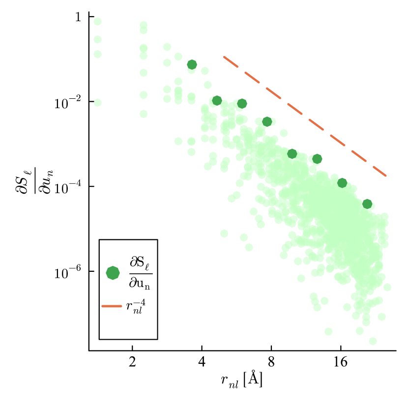
(a) $\delta=0$

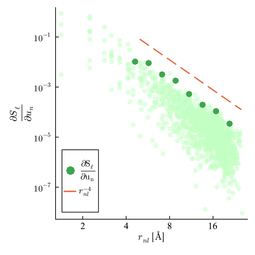
(b) $\delta=0.1$

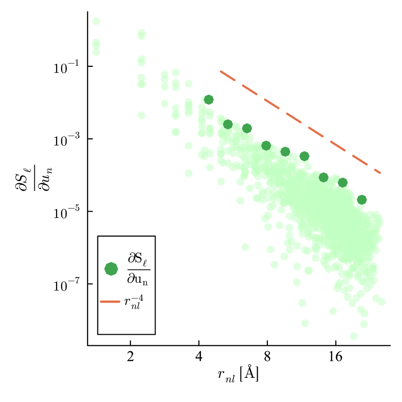
(c) $\delta=0.5$

Figure 3. Derivatives of site entropy for the 2 dimensional toy model including 2025 atoms. The dark green dots represent the maximum $\frac{\partial S}{\partial u_{n}}$ values within specified logarithmic bins along the x axis.

Following the detailed representations of our models, we conducted numerical evaluations of the derivatives of the site entropy, $\left|\frac{\partial S_{\ell}}{\partial u_{n}}\right|$. Figures 2 and 3, demonstrate the rate of decay of site entropies. Our numerical results for the $2D$ model are in good agreement with the predictions made by Theorem 3.1, irrespective of the $\delta$ value. In particular, as we observe larger values of $|r_{n\ell}|$, the magnitude of $\left|\frac{\partial\mathcal{S}_{\ell}(u)}{\partial u_{n}}\right|$ decreases, and this decrease follows the $|r_{n\ell}|^{-4}$ rate indicated by our theory. In the context of the $1D$ model, the numerical outcomes align with theoretical expectations when $\delta=0.1$ and $\delta=0.5$. However, for $\delta=0$, we observed a pre-asymptotic rate of $|r_{n\ell}^{-2}|$, which soon transitions to $|r_{n\ell}^{-1}|$. An enlargement of the domain size revealed that the true rate for this scenario is in fact $|r_{n\ell}^{-1}|$. This can potentially be attributed to the presence of symmetries and cancellation effects in the energy model when the cubic term is disregarded. In summary, our numerical results strongly support the qualitative sharpness of our theory.

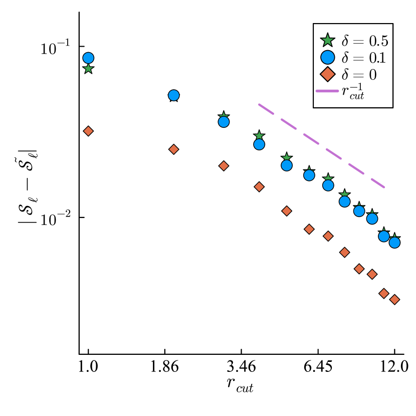
(a) $1$D model

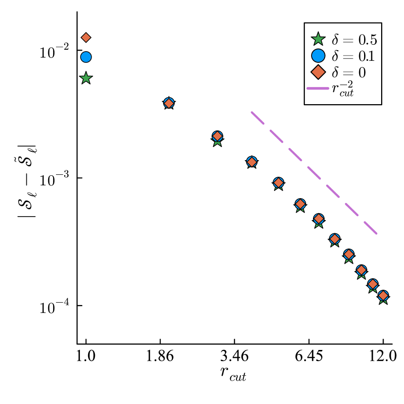
(b) $2$D model

Figure 4. Absolute difference in truncated site entropy $\widetilde{\mathcal{S}}_{\ell}$ and non-truncated site entropy $\mathcal{S}_{\ell}$ for the 1D (left) and 2D (right) toy models with different $\delta$ values. The 1D model included 800 atoms, while the 2D model included 4225 atoms, with the site entropies evaluated near the center of the domains.

Figure 4 illustrates the relationship between the difference in truncated site entropy, denoted as $\widetilde{\mathcal{S}}_{\ell}$, and the non-truncated site entropy, $\mathcal{S}_{\ell}$, as a function of the cutoff radius. This relationship is shown separately for one-dimensional (1D) and two-dimensional (2D) toy models. The observed trend indicates that the reduction in the difference between $\widetilde{\mathcal{S}}_{\ell}$ and $\mathcal{S}_{\ell}$ follows the decay rate $|r_{\rm cut}|^{-d}$, as proposed in theorem 3.1. This trend is consistent across both the 1D and 2D models. This numerically confirms that the truncated site entropy serves as an effective approximation for the non-truncated site entropy and provides a second justification for the surrogate models we will propose in the next section.

It should be noted that the evaluation of site entropy derivatives is computationally demanding. To address this, we adopted an approach to identify the optimal contour and used the sparse nature of the Hessian Jacobians for derivative calculation. The details of this methodology are elaborated in Appendix C. Additionally, all source codes for the numerical tests can be found in our repository .

4. Surrogate Models

The computation of vibrational entropy, as outlined in (2.7) within the harmonic approximation, involves an initial step of determining the Hessian matrix, demanding an $O(N^{2})$ calculation. Subsequently, diagonalizing this matrix incurs a scaling of $O(N^{3})$ for systems comprising $N$ atoms. To address this computational challenge, Lapointe et al. [31] proposed a surrogate model for assessing harmonic vibrational entropy using a linear-in-descriptor machine learning (LDML) approach. While their derivation of entropy closely aligns with the methodology presented in Appendix B, their work lacks a demonstration of the crucial property of locality in site entropy. This property is pivotal as it enables the fitting of entropy using descriptors of atomic environments.

In this section we connect our locality results to learning a surrogate for the site entropy functional. Specifically, we employ the Atomic Cluster Expansion (ACE) framework, and present a series of numerical results pertaining to the fitting of entropy and its applications in materials science.

4.1. Atomic Cluster Expansion (ACE)

Accurate energy and force calculations are best achieved through electronic structure techniques like DFT. However, DFT has limitations for larger systems and longer timescales. To overcome these limitations, machine-learned interatomic potentials (MLIPs), trained on DFT data, have become essential in computational materials science due to their high fidelity [1, 2, 4, 9, 38, 39]. This methodology can be directly transferred to learn surrogate models for entropy.

We utilize the linear atomic cluster expansion (ACE) parameterisation [5]. All in-use MLIPs for materials typically express the total energy, $\mathcal{E}_{\text{ML}}$, as an sum over individual site energies. Leveraging the locality of site entropy, as established in Theorem 3.1, the same approach employed for energy modeling can be seamlessly applied.

To that end, we consider $N$ atoms described by their position vectors $y_{j}$. A set $\mathbf{R}:=\{y_{1},\ldots,y_{N}\}\in\mathbb{R}^{3N}$ of $N$ particle positions is called an atomic configuration. Let $y_{ij}=y_{j}-y_{i}$ be the distances between atom $j$ and a reference atom $i$, and let $\mathbf{y}_{i}=\{y_{ij}\}_{j\neq i}$ represent the atomic neighbourhood around atom $i$. The total entropy of a structure of this kind is broken down into site entropies in the ACE model,

$$S(\mathbf{R})=\sum_{i=1}^{N}S^{*}(\mathbf{y}_{i}),$$ (4.1)

where $S^{*}$ is a site entropy function that depends on its atomic environment $\mathbf{y}_{i}$. The mapping $S:\mathbb{R}^{3N}\to\mathbb{R}$ is permutation- and isometry-invariant, inherited from the same invariance of the energy. Given a cutoff radius $r_{\text{cut}}$, the ACE site entropy $S^{*}$ is expressed as

$$S^{*}(\mathbf{y}_{i};\mathbf{c})=\sum_{B\in\mathcal{B}}c_{B}B\left(\mathbf{y}_{i}\right),$$ (4.2)

with basis functions $B$ and parameters $c_{B}$ that are optimized via a least squares loss minimization. These basis functions are constructed to exhibit invariance under rotations, reflections, and permutations of the atomic environment and are naturally body-ordered, providing a physically interpretable means to converge the fit accuracy. A review of the ACE model and its parameters is given in Appendix D.

To estimate the coefficients when training total entropy, we require a training dataset which contains a list of atomic configuration $\mathfrak{R}=\{\mathbf{R}\}$ for which the total entropy $\mathcal{S}_{\mathbf{R}}\in\mathbb{R}$, and entropy derivatives $\nabla\mathcal{S}_{\mathbf{R}}\in\mathbb{R}^{N\times 3}$ (where $N$ is the total number of atoms in each configuration $\mathbf{R}$) have been evaluated. A possible way to estimate the parameters, closely mimicking parameter estimation for interatomic potentials, is to minimize the quadratic loss function

$$\mathcal{L}(\mathbf{c}):=\sum_{\mathbf{R}\in\mathfrak{R}}\left(\omega^{2}_{S,\mathbf{R}}|S(\mathbf{c};\mathbf{R})-\mathcal{S}_{\mathbf{R}}|^{2}+\omega^{2}_{\nabla S,\mathbf{R}}|\nabla S(\mathbf{c};\mathbf{R})-\nabla\mathcal{S}_{\mathbf{R}}|^{2}\right),$$ (4.3)

with weights $\omega_{S}$ and $\omega_{\nabla S}$ adjusting the significance of the contributions of entropy and its derivatives.

Similarly, to estimate the coefficients when training site entropy on a training dataset $\mathfrak{R}$, we can minimize the following quadratic loss function

$$\mathcal{L}^{*}(\mathbf{c}):=\sum_{\mathbf{R}\in\mathfrak{R}}\left(\omega^{2}_{S^{*},\mathbf{R}}\sum_{i=1}^{N}\left(S^{*}(\mathbf{y}_{i};\mathbf{c})-\mathcal{S}_{i,\mathbf{R}}\right)^{2}+\omega^{2}_{G^{*},\mathbf{R}}\sum_{i=1}^{N}\sum_{j=1}^{3}\sum_{k=1}^{N}\left(G^{*}_{ijk}(\mathbf{c};\mathbf{R})-\mathcal{G}_{ijk,\mathbf{R}}\right)^{2}\right),$$ (4.4)

where $\mathcal{S}_{i,\mathbf{R}}\in\mathbb{R}$ represents the site entropy evaluated at site $i$ and $G^{*}(\mathbf{c};\mathbf{R})\in\mathbb{R}^{N\times 3\times N}$ represents the three-dimensional array with each element $G^{*}_{ijk}$ representing the derivative of the site entropy at site $i$ with respect to the $j$-th spatial dimension of the atom at the $k$-th site. This tensor captures how the contribution of each atom to the overall entropy varies with changes in the positions of all atoms within the system. Similarly, $\mathcal{G}_{ijk,\mathbf{R}}$ denotes the elements of the reference gradient tensor for the site entropy associated with the structure $\mathbf{R}$. The indices $i$, $j$, and $k$ serve the same purposes as described for $G^{*}_{ijk}(\mathbf{c};\mathbf{R})$.

Selecting the appropriate training data, loss functions, and weights, as indicated in the loss function above, is crucial for developing precise models capable of accurate predictions, which will be specified in the following presentation.

4.2. Fitting Entropy

In this section, we will present and discuss the fitting results achieved by using the above mentioned parameterisation of entropy via ACE. We will fit models on both total and site entropies and their respective derivatives. The details on the training and testing procedures will be given below.

4.2.1. Models setup

We start by defining the training set, denoted by $\mathfrak{R}$, which encompasses the collection of training data. Geometry optimization is initially performed on the training domain to find the equilibrium atomic positions. Subsequently, with a chosen parameter $\alpha$ called the rattling parameter, and the number of configurations in $\mathfrak{R}$, denoted as $N_{\text{train}}\equiv|\mathfrak{R}|$, atomic positions are perturbed. Each atom is displaced by a vector with components that are uniformly distributed random numbers within the interval $[-\frac{\alpha}{2},\frac{\alpha}{2}]$. This procedure is repeated $N_{\text{train}}$ times to generate a diverse set of configurations. A similar approach is utilized to generate a test set. The number of configurations for both the training and test sets, $N_{\text{train}}$ and $N_{\text{test}}$, will be detailed for each case study. We choose the weights as $\omega_{S}\gg\omega_{\nabla S}$ to enforce more accuracy on entropy. The parameters $\{c_{B}\}$ are determined by minimizing the loss functions  (4.3) and  (4.4) using a Bayesian Ridge Regression (BLR) [44] solver, which is capable of autonomously determining the importance of input features within the model. The training process utilized open-source Julia packages: JuLIP.jl package for the creation of test and training datasets, as outlined in [16], and ACEpotentials.jl package, detailed in [44] and accessible at [15], for both ACE basis construction and ACE model fitting.

The hyperparamter choices and results are as follows:

• Training and Validation Sets: The dataset includes 100 configurations of rattled Silicon, where each configuration is perturbed by a rattling parameter calculated as $0.1\,\text{\AA}\times U(0,1)$. Here, $U(0,1)$ denotes a random number drawn from a uniform distribution across the interval $(0,1)$. These configurations are encapsulated within a supercell with dimensions $2a_{0}\times 2a_{0}\times a_{0}$ and comprise 32 atoms each, with one vacancy present in every configuration. This set was then split into a training data set including 70 configurations and a validation set including 30 configurations.

• Test Set: The evaluation utilized a test set composed of 100 Silicon configurations, including two groups. The first group contains 50 bulk Silicon configurations, each rattled with a parameter of $0.08\,\text{\AA}\times U(0,1)$. The second group consists of 50 configurations, each including a vacancy and rattled at a parameter of $0.1\,\text{\AA}\times U(0,1)$, refering to the same uniform distribution. The dimensions of the supercell for the test set are identical to those of the training set, maintaining the size of $2a_{0}\times 2a_{0}\times a_{0}$.

• Reference Entropy Calculation: For the purpose of training, the hessian matrices needed to compute site and total entropy and their respective derivatives were computed using the Stillinger-Weber potential [40] implemented in the JuLIP.jl package [16].

• Hyperparameter Tuning: During the fitting process for total entropy, a model with a body order of 3, a maximum polynomial degree of 16, and a cutoff radius of $5.0\,\text{\AA}$ was employed. For site entropy fitting, the chosen model was characterized by a body order of 4, while retaining the same polynomial degree and cutoff radius as used for total entropy fitting. The decision to employ different body orders for each model arose from extensive trial and error. To achieve this, we created 10 different sets including 100 configurations, split into a training set including 70 and a validation set including 30 configurations as described above. We used the training set to fit the models. To find the best combination of body order and degree, we employed a grid search type method and created a grid of body orders (3 and 4) and polynomial degree (8, 10, 12, 14, 16) and evaluated the validation sets’ error on each combination to identify the best setup. After this, a final training set was created and used to train the model that was evaluated on the test sets. This indicates that the hyperparameters were carefully tuned to optimize the model’s performance for each type of entropy fitting.

  The respective weights were chosen as $\omega_{S}=60$ and $\omega_{\nabla S}=1$ when training total entropy, and $\omega_{S_{\ell}}=600$ and $\omega_{\nabla S_{\ell}}=1$ when training site entropy. The slightly higher choice of weights for site entropy is a result of the fact that, when training site entropy, we have $N$ times more derivative data compared to training total entropy, assuming the same number of training configurations are used for both.

The fitting results for both total and site entropies are presented in Figure 5 and Figure 6. For the model fitted to total entropies, the RMSE for the bulk Silicon test set was $1.68\times 10^{-4}\,k_{B}$ for entropy and $1.46\times 10^{-3}\,k_{B}/\text{\AA}$ for its derivatives. For the configurations with a vacancy, the RMSEs were $3.81\times 10^{-4}\,k_{B}$ for entropy and $2.56\times 10^{-3}\,k_{B}/\text{\AA}$ for the derivatives. The RMSE for the model fitted to site entropies for the bulk Silicon test set were $2.58\times 10^{-4}\,k_{B}$, and for the derivatives, $2.47\times 10^{-3}\,k_{B}/\text{\AA}$ and for the test set including a vacancy the RMSEs were $6.71\times 10^{-4}\,k_{B}$, and for the derivatives, $3.95\times 10^{-3}\,k_{B}/\text{\AA}$.

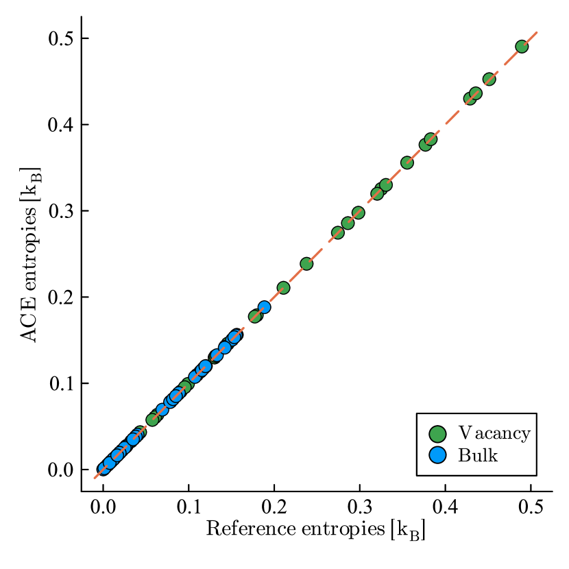
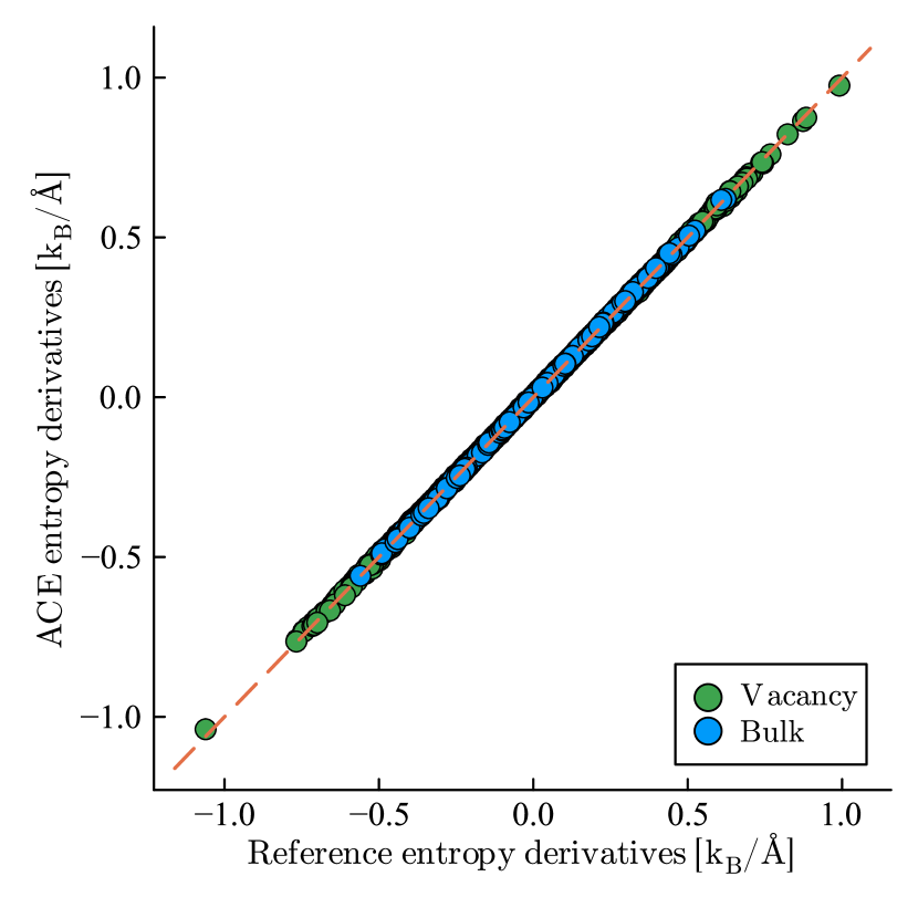
Figure 5. Total entropy trained on 70 configurations including 31 Silicon atoms and tested on 50 rattled configurations of bulk Silicon with a $2a_{0}\times 2a_{0}\times a_{0}$ supercell and and 50 rattled configurations of Silicon including a vacancy.

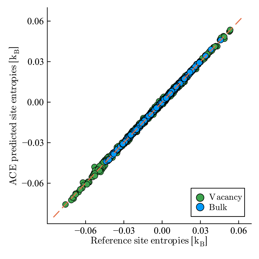
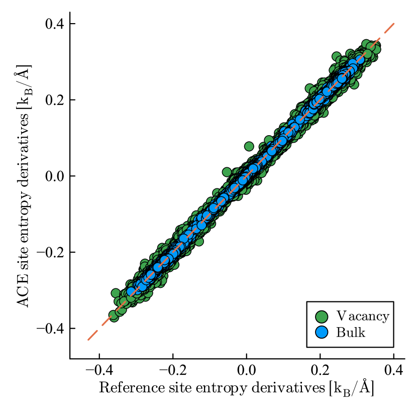
Figure 6. Site entropy trained on 70 configurations including 31 Silicon atoms and tested on 50 rattled configurations of bulk Silicon with a $2a_{0}\times 2a_{0}\times a_{0}$ supercell and and 50 rattled configurations of Silicon including a vacancy.

Additionally, we present a comparison between prediciting total entropy by the means of a model fitted only to total and another one only to site entropies. Our training set in both cases included 50 rattled configurations of Silicon (rattling parameter $=0.1\,\text{\AA}\times U(0,1)$) including a vacancy with a $2a_{0}\times 2a_{0}\times a_{0}$ supercell. Our test set included 50 rattled configurations of bulk Silicon (rattling parameter $=0.08\,\text{\AA}\times U(0,1)$). During the training for total entropy, we constructed a model with a body order of 3, a maximum polynomial degree of 16, and a cutoff radius of $5.0$Å. For the site entropy, we assembeled a model with a body order of 4, a maximum polynomial degree of 16, and a cutoff radius of $5.0$Å. The fitting results are showcased in Figure 7. Consistent with expectations, the task of fitting site entropies presents greater complexity relative to the fitting of total entropies. For the specific objective of predicting total entropies, it is empirically more precise to utilize a model that has been exclusively trained on total entropy data.

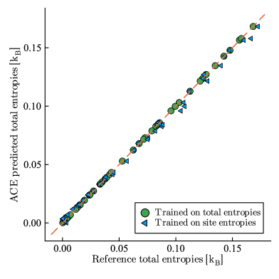
Figure 7. Comparing the performance of two models, one fitted exclusively to total entropy and one fitted solely to site entropy

4.3. Learning curves

We train a series of models with identical hyperparameters except for $r_{\text{cut}}$. The body order and polynomial degree of the trained models were 3 and 14 for total and 3 and 16 for site entropy. Training set sizes are varied within the range of 15 to 200 configurations, ensuring that each set comprises an equal configurations of the four distinct Silicon configuration sets all within a supercell of dimensions $2a_{0}\times 2a_{0}\times a_{0}$: (i) Rattled ($\alpha=0.1\times U(0,1)$) bulk Silicon containing 32 atoms, (ii) Rattled ($\alpha=0.1\times U(0,1)$) Silicon supercell including a single vacancy, (iii) Rattled ($\alpha=0.1\times U(0,1)$) Silicon supercell including a divacancy , and (iv) Rattled ($\alpha=0.1\times U(0,1)$) Silicon supercell including an interstitial. The test set included a total of 80 configurations, with 20 configurations from each aforementioned sets.

Figure 8 and Figure 9 display the log-log plots corresponding to the total and site entropies, respectively. It is noteworthy that upon comparison, we observe that the convergence happens relatively fast for both cases, which is not unexpected due to the simplicity of our training sets. It is also evident that the total entropy values reach convergence earlier when compared to the site entropies. This observation also aligns with expectations, attributed to the inherently lower complexity associated with fitting total entropy. Figure 10 and Figure 11 show the convergence of our fitting with increasing basis size. As the basis size increases, we observe a convergence in both the site and total entropies, along with their respective derivatives, aligning closely with our expectations.

.

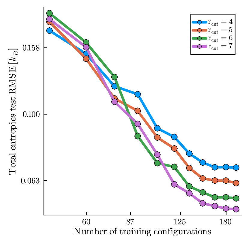
(a) Total entropy

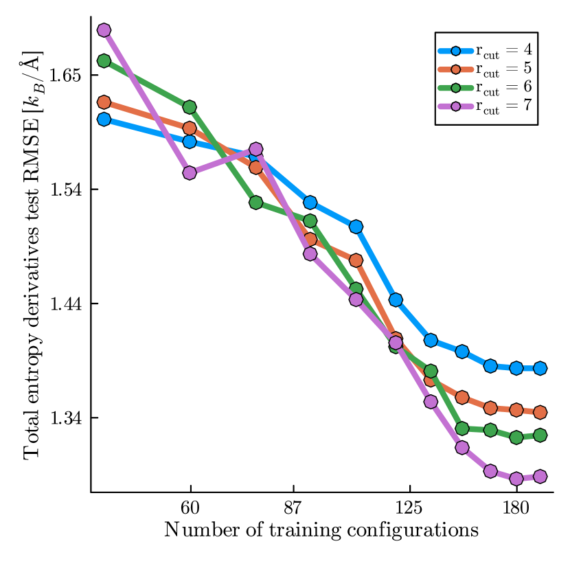
(b) Total entropy derivatives

Figure 8. RMSE Convergence for total entropy varying $r_{cut}$ equal to $4.0\,\text{\AA}$, $5.0\,\text{\AA}$, $6.0\,\text{\AA}$, and $7.0\,\text{\AA}$ for Si. Each point corresponds to $N$ observations corresponding to total entropies and $96\times N$ observations corresponding to total entropy derivatives where $N$ is equal to the number of training configurations.

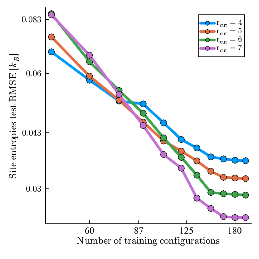
(a) Site entropy

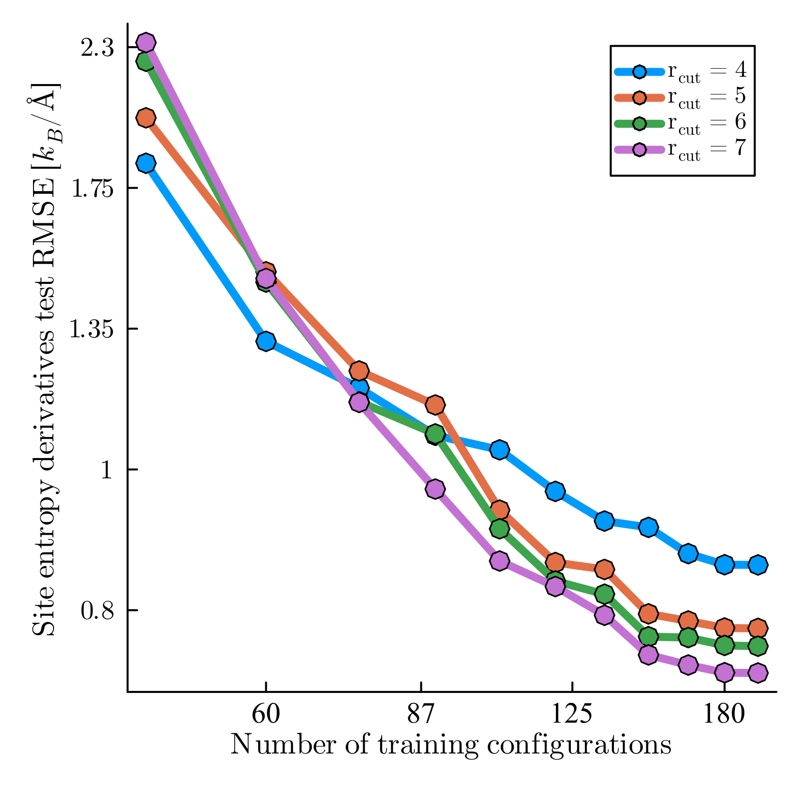
(b) Site entropy derivatives

Figure 9. RMSE Convergence for site entropy varying $r_{cut}$ equal to $4.0\,\text{\AA}$, $5.0\,\text{\AA}$, $6.0\,\text{\AA}$, and $7.0\,\text{\AA}$ for Si. Each point corresponds to $32\times N$ observations corresponding to site entropies and $96\times 32\times N$ observations corresponding to site entropy derivatives where $N$ is equal to the number of training configurations.

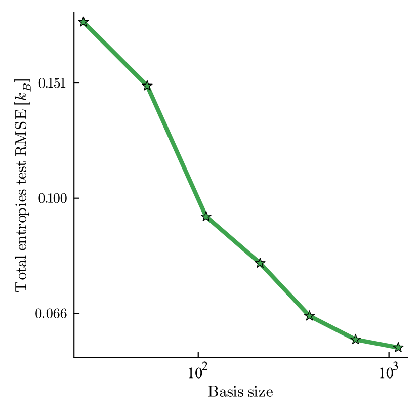
(a) Total entropy

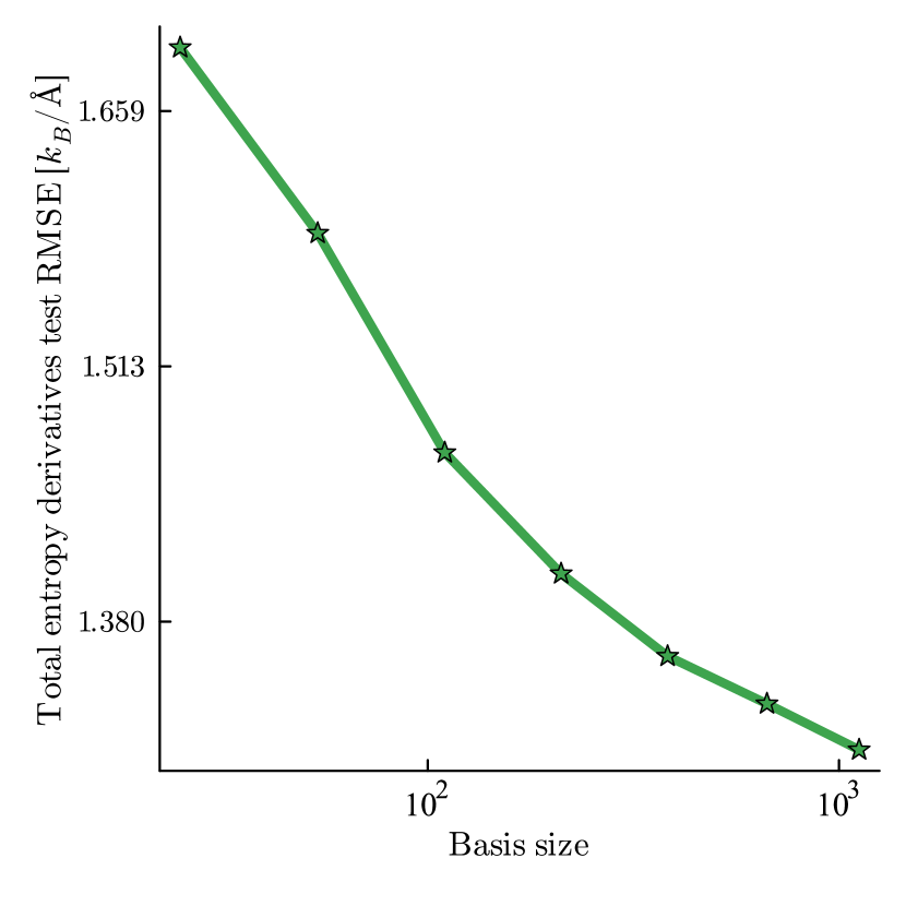
(b) Total entropy derivatives

Figure 10. RMSE Convergence test for total entropy on Si for increasing basis size, fixing the cutoff at 5.5 Å.

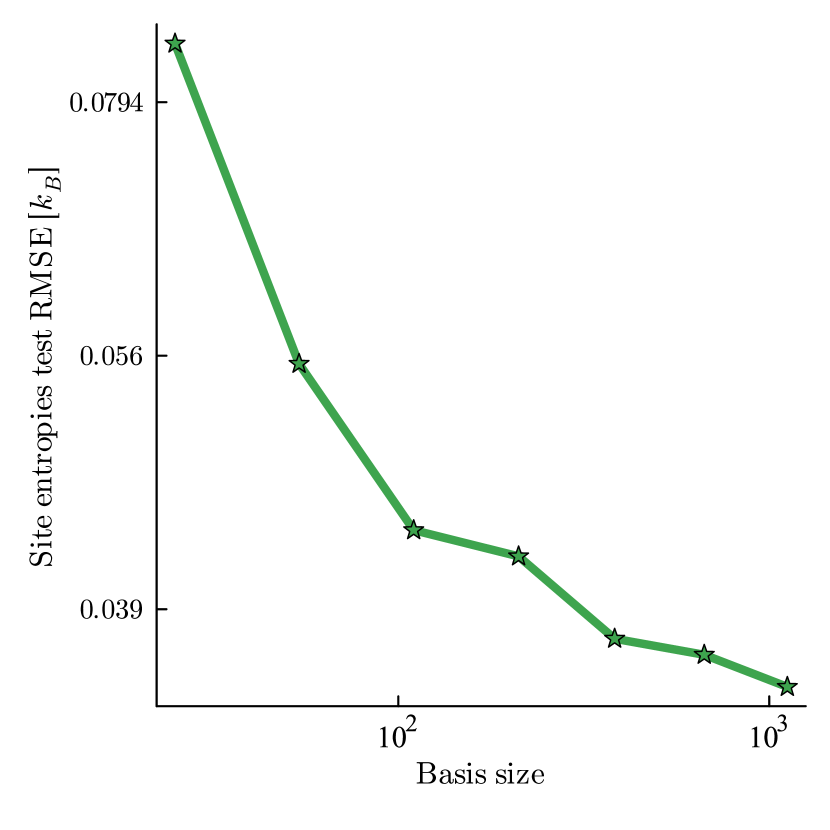
(a) Site entropy

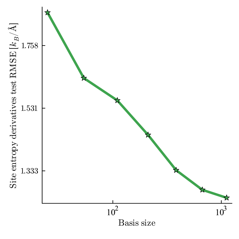
(b) Site entropy derivatives

Figure 11. RMSE Convergence test for site entropy on Si for increasing basis size, fixing the cutoff at 5.5 Å.

4.4. Attempt frequency prediction

An important property related to the vibrational entropy is the transition rate. Within harmonic transition state theory (HTST) it is defined by

$$\mathcal{K}^{\rm HTST}_{N}=\exp\Big{(}-\beta\big{[}\mathcal{F}_{N}(\bar{u}^{\rm saddle}_{N})-\mathcal{F}_{N}(\bar{u}^{\rm min}_{N})\big{]}\Big{)},$$ (4.5)

where, for a critical point $\bar{u}$,

$$\mathcal{F}_{N}(\bar{u})=\mathcal{E}_{N}^{\rm def}(\bar{u})+\beta^{-1}S_{N}(\bar{u}).$$

Notably, in materials modeling, especially for systems operating at temperatures significantly below the melting point, the harmonic approximation is generally deemed reliable [6, 26].

Traditionally, $\mathcal{K}^{\rm HTST}_{N}$ is more typically written as

$$\mathcal{K}^{\rm HTST}_{N}=\bigg{(}\frac{\textstyle\prod\lambda_{j}^{\rm min}}{\textstyle\prod\lambda_{j}^{\rm saddle}}\bigg{)}^{1/2}\,\exp\Big{(}-\beta\big{[}\mathcal{E}_{N}(\bar{u}^{\rm saddle}_{N})-\mathcal{E}_{N}(\bar{u}^{\rm min}_{N})\big{]}\Big{)},$$

where the products involve only the positive eigenvalues of, respectively, the hessians $\nabla^{2}\mathcal{E}_{N}(\bar{u}^{\rm min}_{N})$ and $\nabla^{2}\mathcal{E}_{N}(\bar{u}^{\rm saddle}_{N})$. However, for our purposes, the formulation (4.5) is far more convenient.

To showcase the potential application of our work, we predict the entropic term in the harmonic transition rate (4.5). In case of vacancy migration in a crystal, this term is also called the attempt frequency. The system we considered was Copper in a $2a_{0}\times 2a_{0}\times a_{0}$ supercell including a vacancy. We used an embedded atom model (EAM) potential by Mishin et al. [33], as our reference potential and aimed to predict the attempt frequency of a vacancy migrating from one site to the adjacent one. We obtained the index-1 saddle point and minima using the Nudged Elastic Band (NEB) method [27] implemented in Atomic Simulation Environment (ASE) [32]. We started with a data set including 30 configurations of rattled minima ($\alpha=0.1\times U(0,1)$) and predicted the entropy corresponding to the index-1 saddle point. The RMSE for this prediction was $2.341\;\text{Hz}$. We then added the un-rattled index-1 saddle point to the data set, the error for that prediction is shown in Figure 12. After that, we removed the index-1 saddle point and gradually added rattled saddle points ($\alpha=0.1\times U(0,1)$) to the training set and compute the RMSE as demonstrated in Figure 12 in a log-log plot. Our test set included 30 rattled saddle points ($\alpha=0.1\times U(0,1)$). To train the models, we used a body order of 3 and a polynomial degree of 12. The aim of the gradual adding of rattled saddle points is to add more information about the area between the minima and the saddle point to the model. It is evident that adding more saddle configurations to the training set effects the accuracy of the prediction tremendously.

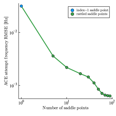
Figure 12. Attempt frequency of a vacancy migrating from one site to the adjacent one in Copper. The index-1 saddle point shows the error for a model trained on 30 rattled minima and the index-1 saddle point.

5. Conclusion

In this work, we have demonstrated that the total energy can be decomposed into atomic site contributions and have rigorously estimated the locality of site entropy. Our analysis suggests that vibrational entropy can be accurately predicted using a surrogate model for site entropy, which we have developed using machine learning techniques, specifically employing the Atomic Cluster Expansion (ACE) model. Our numerical experiments primarily focus on point defects such as vacancies and interstitials. We have showcased the robustness of our approach in predicting vibrational entropy and the attempt frequency for transition rates governing point defect migration, which is a critical aspect of transition state theory rate approximations.

While the current study emphasizes the effectiveness of our approach in a relatively straightforward context, it also enables a detailed and rigorous examination, albeit within certain limitations. There are numerous potential generalizations that can be explored, including extending the methodology to more intricate material and defect geometries. Additionally, our results pave the way for predicting various entropy-dependent physical quantities, including but not limited to dynamical properties such as diffusion coefficients.

Appendix A Proofs

In this section, we begin by introducing the necessary concepts and models within the primary context of this work. We accomplish this by conducting a comprehensive review of the framework proposed in [10, 13], while also adapting their approaches to align with the specific objectives of our current work.

A.1. Preliminaries

First of all, we introduce the semi-discrete Fourier transform (SDFT)

$$\hat{u}(k):=\sum_{\ell\in\Lambda}e^{ik\ell}\cdot u(\ell),\quad\text{with inverse}\quad u(\ell)=\frac{1}{|\mathcal{B}|}\int_{\mathcal{B}}e^{-ik\ell}\cdot\hat{u}(k)\,{\rm d}k,$$ (A.1)

where $\mathcal{B}=\pi{\sf A}^{-T}(-1,1)^{d}$ is a fundamental domain of reciprocal space (equivalent to the first Brillouin zone) and has the volume $\lvert\mathcal{B}\rvert=\frac{(2\pi)^{d}}{\lvert\det{\sf A}\rvert}$.

We now review a characterization of F, which plays a key role in proving our main locality theory (cf. Theorem 3.1). Since $H^{\rm hom}$ is circulant, we can represent ${\rm\textbf{F}}\omega=F*\omega$ and define $F$ via its Fourier transform.

To that end, we recall that

$$\langle H^{\rm hom}u,v\rangle=\sum_{\ell\in\mathbb{Z}^{d}}\nabla^{2}V({\bf 0})\big{[}Du(\ell),Dv(\ell)\big{]},$$

then applying the SDFT we obtain

$$\langle H^{\rm hom}u,v\rangle=\frac{1}{\mathcal{B}}\int_{\mathcal{B}}\hat{u}(k)^{*}\hat{h}(k)\hat{v}(k)\,{\rm d}k$$ (A.2)

with

$$a^{T}\hat{h}(k)b:=\nabla^{2}V({\bf 0})\big{[}\big{(}(e^{-ik\rho}-1)a\big{)}_{\rho\in\mathcal{R}},\big{(}(e^{ik\rho}-1)b\big{)}_{\rho\in\mathcal{R}}\big{]}.$$

One can also reduce $\hat{h}(k)$ to the simpler form

$$\hat{h}(k)=4\sum_{\rho\in\mathcal{R}^{\prime}}A_{\rho}\cdot\sin^{2}\left(\frac{k\cdot\rho}{2}\right)$$

with $\mathcal{R}^{\prime}=(\mathcal{R}\cup\{0\})+(\mathcal{R}\cup\{0\})$, see [13, Section 6.2] for more details. Moreover, the stability implies that $c_{0}|k|^{2}\cdot\mathsf{I}\leq\hat{h}(k)\leq c_{1}|k|^{2}\cdot\mathsf{I}$ with the identity matrix $\mathsf{I}$ for all $k\in\mathcal{B}$ [28]. We observe that $|\hat{h}(k)^{-1/2}|\lesssim|k|^{-1}$ as $|k|\rightarrow 0$, hence we can define

$$F(\ell) :=\frac{1}{|\mathcal{B}|}\int_{\mathcal{B}}e^{-ik\ell}\cdot\hat{F}(k)\,{\rm d}k,\qquad\text{where}\quad\hat{F}(k)=\hat{h}(k)^{-1/2},$$ (A.3)

$$(\boldsymbol{\rm F}u)(\ell) :=\sum_{m\in\Lambda}\big{(}F(\ell-m)-F(-m)\big{)}u(m).$$ (A.4)

The constant shift $\sum_{m}F(-m)u(m)$ in the definition of F$u$ ensures that F$u$ is well-defined [6].

The following lemma presents key properties of the operator F, which holds a pivotal role in our framework. We state it here to ensure the completeness of our presentation.

Lemma A.1. [6, Lemma 3.1] Let $F:\Lambda\to\mathbb{R}^{m\times m}$ and F be defined by (A.3) and (A.4), respectively. Then, we have: (i) for any $\bm{\rho}\in\mathcal{R}^{j}$, $j\geq 0$, there exists a constant $C$ such that

$$|D_{\bm{\rho}}F(\ell)|\leq C(1+|\ell|)^{1-d-j}\quad\forall\ell\in\mathbb{Z}^{d}.$$

(ii) F $\in\mathcal{L}\big{(}\ell^{2},\dot{\mathcal{W}}^{1,2}\big{)}$. (iii) F${}^{*}H^{\rm hom}$F $=I$, understood as operators $\ell^{2}\to\ell^{2}$.

A crucial quantity for proving locality is the estimation of the resolvent $\mathscr{R}_{z}(u)=(zI-\boldsymbol{\rm F}^{*}H(u)\boldsymbol{\rm F})^{-1}$. Before providing this estimate, we first review a useful lemma.

Lemma A.2. [6, Lemma 3.3 (i)] Let $X$ be a Hilbert space. Let $A\in\mathcal{L}(X,X)$ be a bounded linear operator with range of finite dimension at most $r\in\mathbb{N}$ and $I+A$ is invertible, then there exist $c_{1}(A),\dots,c_{r+1}(A)\in\mathbb{R}$ such that

$$(I+A)^{-1}=I+\sum_{j=1}^{r+1}c_{j}(A)A^{j}.$$ (A.5)

As discussed in Section 2.4, we are ready to give the estimate of resolvent $\mathscr{R}_{z}(u)$ for $u\in\mathcal{U}$, where

$$\mathcal{U}(\underline{\sigma},\overline{\sigma}):=\big{\{}u\in\dot{\mathcal{W}}^{1,2}:\sigma\big{[}\boldsymbol{\rm F}^{*}H(u)\boldsymbol{\rm F}\big{]}\cap(0,\infty)\subset[\underline{\sigma},\overline{\sigma}]\big{\}},$$

with $0<\underline{\sigma}<\overline{\sigma}$ fixed throughout this work and all constants in the following are allowed to depend on them.

Lemma A.3. Let $\mathscr{R}_{z}(u)$ be the resolvent operator defined by (2.21). Then for all $u\in\mathcal{U}$ there exists a constant $C_{1}>0$ independent of $m$ or $n$, such that

$$\big{|}[\mathscr{R}_{z}(u)]_{mn}\big{|}\leq C_{1}\big{(}1+|r_{mn}|\big{)}^{-d}.$$ (A.6)

Proof.

The main technique we use is to decompose a Hessian operator $H$ into two components $H=H^{\rm d}+H^{\rm h}$ where $H^{\rm d}$ as finite rank and represents the defect core while $H^{\rm h}$ is close to $H^{\text{hom}}$ and thus represents the far-field.

We begin by splitting the difference of the hessians $H(u)-H^{\text{hom}}$ into a sum of a finite rank operator representing the defect core and an infinite rank part representing the far field. To that end, given $M$ sufficiently large, we denote

$$\langle H^{M}(u)v,z\rangle:=\sum_{\lvert\ell\rvert\leq M}\nabla^{2}V({\bf 0})\big{[}Dv(\ell),Dz(\ell)\big{]}+\sum_{\lvert\ell\rvert>M}\nabla^{2}V(Du(\ell))\big{[}Dv(\ell),Dz(\ell)\big{]}.$$ (A.7)

The resolvent $\mathscr{R}_{z}$ can be decomposed as follows:

$$\mathscr{R}_{z}=(zI-\boldsymbol{\rm F}^{*}H(u)\boldsymbol{\rm F})^{-1}= ~{}\Big{[}zI-\boldsymbol{\rm F}^{*}H^{M}(u)\boldsymbol{\rm F}+\boldsymbol{\rm F}^{*}H^{M}(u)\boldsymbol{\rm F}-\boldsymbol{\rm F}^{*}H(u)\boldsymbol{\rm F}\Big{]}^{-1}$$ (A.8)

$$= ~{}\Big{[}\big{(}zI-\boldsymbol{\rm F}^{*}H^{M}(u)\boldsymbol{\rm F}\big{)}+\boldsymbol{\rm F}^{*}\big{(}H^{M}(u)-H(u)\big{)}\boldsymbol{\rm F}\Big{]}^{-1}$$

$$= ~{}\Big{[}(\mathscr{R}_{z}^{M})^{-1}+\boldsymbol{\rm F}^{*}\big{(}H^{M}(u)-H(u)\big{)}\boldsymbol{\rm F}\Big{]}^{-1}$$

$$= ~{}\Big{[}(\mathscr{R}_{z}^{M})^{-1}\big{(}I+\mathscr{R}_{z}^{M}\boldsymbol{\rm F}^{*}\big{(}H^{M}(u)-H(u)\big{)}\boldsymbol{\rm F}\big{)}\Big{]}^{-1}$$

$$= ~{}\Big{[}I+\mathscr{R}_{z}^{M}\boldsymbol{\rm F}^{*}\big{(}H^{M}(u)-H(u)\big{)}\boldsymbol{\rm F}\Big{]}^{-1}\cdot\mathscr{R}_{z}^{M}$$

$$:= ~{}\big{(}I+B^{M}\big{)}^{-1}\cdot\mathscr{R}_{z}^{M},$$

where $\mathscr{R}_{z}^{M}=\big{(}zI-\boldsymbol{\rm F}^{*}H^{M}(u)\boldsymbol{\rm F}\big{)}^{-1}$.

Since the resolvent $\mathscr{R}_{z}(u)$ exists for all $z\in\mathbb{C},u\in\mathcal{U}$, the inverse on the right hand side exists as well. Additionally, the term $B^{M}:=\mathscr{R}_{z}^{M}\boldsymbol{\rm F}^{*}\big{(}H^{M}(u)-H(u)$ has finite-dimensional range since this is clearly the case for $H^{M}(u)-H(u)$. Thus, according to Lemma A.5 it follows that

$$\big{(}I+B^{M}\big{)}^{-1}=I+\sum_{j=1}^{r+1}c_{j}(B^{M})\big{(}B^{M}\big{)}^{j}.$$

The constants $c_{j}$ remain uniformly bounded in $z,u\in\mathcal{U}$, therefore we only need to estimate

$$\big{(}B^{M}\big{)}^{j}\mathscr{R}_{z}^{M}=\big{(}\mathscr{R}_{z}^{M}\boldsymbol{\rm F}^{*}\big{(}H^{M}(u)-H(u)\big{)}\boldsymbol{\rm F}\big{)}^{j}\mathscr{R}_{z}^{M},$$ (A.9)

for $1\leq j\leq r+1$. Using the techniques shown in [6, Eq. (7.13)], one can obtain

$$\left|\Big{(}\boldsymbol{\rm F}^{*}\big{(}H^{M}(u)-H(u)\big{)}\boldsymbol{\rm F}\Big{)}_{mn}\right|\lesssim \sum_{\lvert\ell\rvert\leq M}(\lvert\ell\rvert+1)^{-d}(\lvert\ell-m\rvert+1)^{-d}(\lvert\ell-n\rvert+1)^{-d}$$ (A.10)

$$\leq \sum_{\ell}(\lvert\ell\rvert+1)^{-d}(\lvert\ell-m\rvert+1)^{-d}(\lvert\ell-n\rvert+1)^{-d}$$

$$\lesssim (|n|+1)^{-d}(|n-m|+1)^{-d}+(|m|+1)^{-d}(|n-m|+1)^{-d}$$

$$+(|n|+1)^{-d}(|m|+1)^{-d}.$$

Hence, applying [6, Eq. (3.19) and Eq. (3.26)], we have

$$\big{|}\big{[}\mathscr{R}_{z}\big{]}_{mn}\big{|}=\left|\big{[}\big{(}\mathscr{R}_{z}^{M}\boldsymbol{\rm F}^{*}\big{(}H^{M}(u)-H(u)\big{)}\boldsymbol{\rm F}\big{)}^{j}\mathscr{R}_{z}^{M}\big{]}_{mn}\right|\leq C_{1}(1+|r_{mn}|)^{-d},$$

where $C_{1}>0$ is independent of $m$ or $n$. This completes the proof. ∎

We are ready to give the proof of our main theorem (cf. Theorem 3.1).

Proof of Theorem 3.1.

The site entropy $\mathcal{S}_{\ell}(u)$ can be expressed using the contour integral defined in (2.22),

$$\mathcal{S}_{\ell}(u):=-\frac{1}{2}\frac{1}{2\pi i}{\rm Trace}\left[\oint_{\mathcal{C}}\log^{+}(z)\cdot\big{(}zI-\mathbf{F}^{*}H(u)\mathbf{F}\big{)}^{-1}\,{\rm d}z\right]_{\ell\ell},$$ (A.11)

where $\mathscr{R}_{z}:=\big{(}zI-\mathbf{F}^{*}H(u)\mathbf{F}\big{)}^{-1}$. Differentiating with respect to $u$, we get

$$\frac{\partial\mathcal{S}_{\ell}(u)}{\partial u} =-\frac{1}{2}\frac{1}{2\pi i}\oint_{\mathcal{C}}\log^{+}(z)\cdot{\rm Trace}\left[\mathscr{R}_{z}\mathbf{F}^{*}\frac{\partial H(u)}{\partial u}\mathbf{F}\mathscr{R}_{z}\right]_{\ell\ell}\,{\rm d}z.$$ (A.12)

The first and second variations of $\mathcal{E}(u)$ are defined as follows:

$$\langle\delta\mathcal{E}(u),v\rangle =\sum_{\ell\in\Lambda}\sum_{\rho\in\mathcal{R}}V_{,\rho}\big{(}Du(\ell)\big{)}\cdot D_{\rho}v(\ell),$$

$$\langle\delta^{2}\mathcal{E}(u)v,w\rangle =\sum_{\ell\in\Lambda}\sum_{\rho,\sigma\in\mathcal{R}}V_{,\rho\sigma}\big{(}Du(\ell)\big{)}\cdot D_{\rho}v(\ell)D_{\sigma}w(\ell).$$

Hence, we can write

$$\langle\delta^{2}\mathcal{E}(u)\textbf{F}^{\alpha},\textbf{F}^{\beta}\rangle=\sum_{\ell\in\Lambda}\sum_{\rho,\sigma\in\mathcal{R}}V_{,\rho\sigma}\big{(}Du(\ell)\big{)}\cdot D_{\rho}\textbf{F}^{\alpha}(\ell)D_{\sigma}\textbf{F}^{\beta}(\ell).$$

According to (A.1), we have

$$\frac{\partial}{\partial u_{n}}\Big{[}\textbf{F}^{*}H(u)\textbf{F}\Big{]}_{\alpha\beta}=\sum_{\ell\in\Lambda}\sum_{\rho,\sigma,\tau\in\mathcal{R}}V_{,\rho\sigma\tau}\big{(}Du(\ell)\big{)}\cdot D_{\rho}\textbf{F}^{\alpha}(\ell)D_{\sigma}\textbf{F}^{\beta}(\ell)D_{\tau}e_{n}(\ell).$$ (A.13)

Hence, one can acquire

$$\Big{|}\frac{\partial}{\partial u_{n}}\Big{[}\textbf{F}^{*}H(u)\textbf{F}\Big{]}_{\alpha\beta}\Big{|} \lesssim\sum_{\ell\in\Lambda}\Big{(}\sum_{\rho\in\mathcal{R}}\big{|}D_{\rho}\textbf{F}^{\alpha}(\ell)\big{|}^{2}\Big{)}^{1/2}\Big{(}\sum_{\sigma\in\mathcal{R}}\big{|}D_{\sigma}\textbf{F}^{\beta}(\ell)\big{|}^{2}\Big{)}^{1/2}\Big{(}\sum_{\tau\in\mathcal{R}}\big{|}D_{\tau}e_{n}(\ell)\big{|}^{2}\Big{)}^{1/2}$$ (A.14)

$$\lesssim\sum_{n\in\Lambda}\big{|}DF(n-\alpha)\big{|}\cdot\big{|}DF(n-\beta)\big{|}$$

$$\lesssim\sum_{n\in\Lambda}|n-\alpha|^{-d}|n-\beta|^{-d},$$

where the last inequality follows from Lemma A.1. Applying Lemma  A.1, we have

$$\left[\mathscr{R}_{z}\frac{\partial}{\partial u_{n}}\Big{[}\textbf{F}^{*}H(u)\textbf{F}\Big{]}_{\alpha\beta}\mathscr{R}_{z}\right]_{\ell\ell} \lesssim\sum_{{\alpha,\beta}\in\Lambda}|\alpha-\ell|^{-d}|\beta-\ell|^{-d}|n-\alpha|^{-d}|n-\beta|^{-d}$$ (A.15)

$$\lesssim\Big{(}\sum_{{\alpha}\in\Lambda}|\alpha-\ell|^{-d}|n-\alpha|^{-d}\Big{)}^{2}$$

$$\lesssim\Big{(}\int_{1}^{|n-\ell|}r^{-d}r^{d-1}|n-\ell|^{-d}\,{\rm d}r\Big{)}^{2}+\int_{|n-\ell|}^{\infty}r^{d-1}r^{-2d}\,{\rm d}r$$

$$\lesssim|n-\ell|^{-2d}.$$

We can now estimate the derivative of the site entropy as

$$\left|\frac{\partial\mathcal{S}_{\ell}(u)}{\partial u_{n}}\right| \leq\frac{1}{2}\frac{1}{2\pi i}\mathrm{Trace}\left|\oint_{\mathcal{C}}\log^{+}(z)\cdot\left[\mathscr{R}_{z}\mathbf{F}^{*}\frac{\partial H(u)}{\partial u_{n}}\mathbf{F}\mathscr{R}_{z}\ \right]_{\ell\ell}{\rm d}z\right|$$ (A.16)

$$\lesssim\frac{1}{4\pi i}\oint_{\mathcal{C}}\big{|}\log^{+}(z)\big{|}\cdot|n-\ell|^{-2d}\,{\rm d}z$$

$$\leq C_{2}|n-\ell|^{-2d},$$

where $C_{2}>0$ is a constant. Let $r_{n\ell}:=|n-\ell|^{-2d}$. We can then establish the locality as stated in Theorem 3.1, thus completing the proof. ∎

Proof of Theorem 3.1.

For $u\in\dot{\mathcal{W}}^{1,2}$, we consider the Taylor expansion of $\widetilde{\mathcal{S}}^{+}_{\ell}$ at the reference homogeneous lattice, that is,

$$\widetilde{\mathcal{S}}_{\ell}(u)=\widetilde{\mathcal{S}}_{\ell}({\bf 0})+\sum_{m\in\Lambda}\frac{\partial\widetilde{\mathcal{S}}_{\ell}({\bf 0})}{\partial u_{m}}\cdot u_{m}+\text{higher order terms}.$$ (A.17)

According to the definition (3.3), the difference in site entropy can be estimated by

$$\left|\mathcal{S}_{\ell}(u)-\widetilde{\mathcal{S}}_{\ell}(u)\right| \leq\left|\sum_{|r_{\ell m}|>r_{\rm cut}}\frac{\partial\mathcal{S}_{\ell}({\bf 0})}{\partial u_{m}}u_{m}\right|$$

$$\leq\|u\|_{L^{\infty}}\cdot\sum_{|r_{\ell m}|>r_{\rm cut}}\left|\frac{\partial\mathcal{S}^{+}_{\ell}({\bf 0})}{\partial u_{m}}\right|.$$ (A.18)

Next, we employ Theorem 3.1 to estimate the decay of the derivatives of the site entropy. Specifically, we can write

$$\left|\mathcal{S}_{\ell}(u)-\widetilde{\mathcal{S}}_{\ell}(u)\right| \leq\|u\|_{L^{\infty}}\cdot\sum_{|r_{\ell m}|>r_{\rm cut}}C_{2}|r_{\ell m}|^{-2d}$$

$$\leq C_{3}\|u\|_{L^{\infty}}\cdot\int_{|r_{\ell m}|\leq r_{\rm cut}}|r_{\ell m}|^{-2d}\,\mathrm{d}V$$

$$\leq C_{3}\|u\|_{L^{\infty}}\cdot\int_{0}^{r_{\rm cut}}r^{-2d}\cdot r^{d-1}\,\mathrm{d}r,$$ (A.19)

where $\mathrm{d}V$ represents the volume element in the $d$-dimensional space. This can be estimated in terms of the cut-off radius $r_{\rm cut}$, resulting in the bound

$$\left|\mathcal{S}_{\ell}(u)-\widetilde{\mathcal{S}}_{\ell}(u)\right| \leq C_{3}\|u\|_{L^{\infty}}\cdot r_{\rm cut}^{-d},$$ (A.20)

where $C_{3}$ is a constant that depends on the volume of the integration domain and the constant $C_{2}$ from Theorem 3.1. ∎

Appendix B An alternative derivation of entropy

In this section, we provide an alternative derivation of site entropy commonly used in physics and engineering [19, 36]. Expanding on our discussion of lattice displacements from a classical standpoint in Section 2.2, we now delve into a quantum mechanical perspective, assuming that a lattice vibration mode with frequency $\omega$ behaves like a simple harmonic oscillator, thereby being confined to specific energy values. We will show that this derivation yields the same definition for entropy mentioned in Section 2.2.

To that end, we first consider a harmonic oscillator with energy levels given by:

$$E_{n}=\hbar\omega\left(n+\frac{1}{2}\right),$$ (B.1)

where $\hbar$ is the reduced Planck constant, and $\omega$ is the angular frequency. The partition function for the quantum harmonic oscillator is the sum of the Boltzmann factors for all possible states [19], that is,

$$Z(\omega)=\sum_{n=0}^{\infty}e^{-\beta E_{n}}=e^{-\beta\hbar\omega/2}\cdot\sum_{n=0}^{\infty}e^{-\beta\hbar\omega n}=\frac{e^{-\beta\hbar\omega/2}}{1-e^{-\beta\hbar\omega}},$$ (B.2)

where the last identity follows from the results of infinite geometric series and $\beta:=1/(k_{B}T)$.

Using the definition of Helmholtz free energy defined by (2.7), we can obtain

$$\mathcal{A}(\omega) =-\frac{1}{\beta}\log\big{(}Z(\omega)\big{)}$$ (B.3)

$$=-\frac{1}{\beta}\left(-\frac{\beta\hbar\omega}{2}-\log(1-e^{-\beta\hbar\omega})\right)$$

$$=\frac{1}{2}\hbar\omega+\frac{1}{\beta}\log(1-e^{-\beta\hbar\omega}).$$

Suppose that we have already obtained all the eigenstates $|\phi\rangle$ and eigenvalues $\omega_{\alpha}^{2}$ of the Hessian $H$, obtained through $(H-M\omega_{\alpha}^{2})|\phi\rangle=|0\rangle$. Then, we define the total density of states (DOS) [18] by

$$\Omega(\omega):=\sum_{\alpha=1}^{3N}\delta(\omega-\omega_{\alpha}).$$ (B.4)

The DOS can be comprehended in the operational sense that if we integrate $\Omega(\omega)$ over a frequency range $\omega_{1}$ to $\omega_{2}$, we therefore obtain the total number of states within that frequency range [24]

$$\langle\Omega(\omega),f\rangle=\int f(\omega)\Omega(\omega)\;\mathrm{d}\omega=\sum_{\alpha=1}^{3N}f(\omega_{\alpha})\quad\text{for}\;f\in C(\mathbb{R}).$$ (B.5)

Hence, for a system of $N$ atoms with $3N$ degrees of freedom, we expect $\int_{0}^{\infty}\Omega(\omega)\,\mathrm{d}\omega=3N$. Using (B.5), we can now determine the overall free energy of the system, $\mathcal{A}_{\text{total}}$, accounting for all vibrational modes as follows:

$$\mathcal{A}_{\text{total}}=\sum_{\alpha=1}^{3N}\mathcal{A}(w_{\alpha})=\int_{0}^{\infty}\mathcal{A}(\omega)\Omega(\omega)\,\mathrm{d}\omega.$$ (B.6)

Substituting (B.3) into (B.6), one can obtain

$$\mathcal{A}_{\text{total}}=\int_{0}^{\infty}\left(\frac{1}{2}\hbar\omega+k_{B}T\log(1-e^{-\beta\hbar\omega})\right)\Omega(\omega)\,\mathrm{d}\omega.$$ (B.7)

Now, we can compute the derivative of $\mathcal{A}_{\text{total}}$ with respect to temperature to acquire the total entropy, that is,

$$\mathcal{S}_{\text{total}}=k_{B}\int_{0}^{\infty}\left[\frac{\beta\hbar\omega}{e^{\beta\hbar\omega}-1}-\log(1-e^{-\beta\hbar\omega})\right]\Omega(\omega)\,\mathrm{d}\omega.$$ (B.8)

In the classical limit of high temperatures, specifically when the temperatures exceed the crystal’s Debye temperature such that $\frac{\hbar\omega}{k_{B}T}\ll 1$, (B.8) asymptotically approaches to

$$\mathcal{S}_{\text{total}} =k_{B}\int_{0}^{\infty}\left[\log\left(\frac{kT}{\hbar\omega_{\alpha}}\right)+1\right]\Omega(\omega)\,\mathrm{d}\omega.$$ (B.9)

To determine defect formation entropy, we need to assess the change in the total density of states (DOS) due to the presence of defect, i.e.,

$$\mathcal{S}^{\rm defect}-S^{\rm ideal}=k_{B}\int_{0}^{\infty}\left[\log\left(\frac{kT}{\hbar\omega_{\alpha}}\right)+1\right]\Delta\Omega(\omega)\,\mathrm{d}\omega,$$ (B.10)

where the term $\Delta\Omega(\omega)$ represents the difference in DOS introduced by the defect, defined as $\Delta\Omega(\omega)=\Omega^{0}(\omega)-\Omega(\omega)$. Here, $\Omega^{0}(\omega)$ and $\Omega(\omega)$ denote the total DOS of the defect and ideal lattice, respectively.

In the case where the defect does not add additional degrees of freedom to the lattice, e.g. for a substitutional defect, we have

$$\int_{0}^{\infty}\Delta\Omega(\omega)\ \mathrm{d}\omega=0,$$

which leads to the fact that

$$\Delta\mathcal{S}=\mathcal{S}^{\rm defect}-\mathcal{S}^{\rm ideal}=-k_{B}\int_{0}^{\infty}\log(\omega)\Delta\Omega(\omega)\,\mathrm{d}\omega.$$ (B.11)

We can use the equivalent representations for  (B.4) and write

$$\Delta\Omega(\omega) =\sum_{\alpha}\big{(}\delta(\omega-\omega_{\alpha})-\delta(\omega-\omega_{\alpha}^{0})\big{)}$$ (B.12)

$$=2\omega\;\mathrm{Trace}\big{(}\delta(\omega^{2}-H)-\delta(\omega^{2}-H_{0})\big{)}.$$

Thus, the defect formation entropy is

$$\Delta\mathcal{S}=\frac{k_{B}}{2}\sum_{\alpha=1}^{3N}\;\log\frac{(\omega_{\alpha}^{0})^{2}}{(\omega_{\alpha})^{2}}=\frac{k_{B}}{2}\;\mathrm{Trace}(\log H_{0}-\log H)=\frac{k_{B}}{2}\;\log(\frac{\mathrm{det}\;H_{0}}{\mathrm{det}\;H}),$$ (B.13)

which is identical to our derivation  (2.7) shown in the main context.

Finally, we are in the stage of considering the spatial decomposition of $\Omega$ which would automatically lead to a spatial decomposition of $S$. Following the discussion in [36], we have

$$\Omega_{\ell}(\omega)=\sum_{\alpha}\delta(\omega-\omega_{\alpha})[\phi_{\alpha}]_{\ell}^{2},$$ (B.14)

where $[\phi_{\alpha}]_{\ell}$ is the $\ell$-th entry of $\phi_{\alpha}$. Using (B.9) and (B.14), we can decompose the total entropy into local contributions from individual atoms,

$$\mathcal{S}_{\ell}(\omega):=\langle\Omega_{\ell}(\omega),\xi\rangle=\sum_{\alpha=1}^{3N}\xi(\omega_{\alpha})[\phi_{\alpha}]_{\ell}^{2}\quad\text{where}\ \xi:=k_{B}\left[\log\left(\frac{kT}{\hbar\omega_{\alpha}}\right)+1\right].$$ (B.15)

It is straightforward to verify that

$$\mathcal{S}_{\text{total}}=\sum_{\ell\in\Lambda}\mathcal{S}_{\ell}=k_{B}\sum_{\alpha=1}^{3N}\left[\log\left(\frac{kT}{\hbar\omega_{\alpha}}\right)+1\right][\phi_{\alpha}]_{\ell}^{2}.$$ (B.16)

We have shown that in the local basis, total entropy can be accurately partitioned into site-specific contributions. This local entropy is essential for understanding the thermodynamic properties of materials at the atomic level. Thus, the locality principle is not just a mathematical convenience but a reflection of the physical reality of how atomic vibrations contribute to the overall entropy of a system.

Appendix C Fast contour integration

We first recall that the definition of total entropy introduced in Section 2.3, that is,

$$\mathcal{S}(u):= -\frac{1}{2}\operatorname{Trace}\,\log(\textbf{F}^{*}H(u)\textbf{F})$$

$$= -\frac{1}{2}\frac{1}{2\pi i}\oint_{\mathcal{C}}\log(z)\cdot{\rm Trace}\big{(}z\mathbf{I}-\boldsymbol{\rm F}^{*}H(u)\boldsymbol{\rm F}\big{)}^{-1}\,{\rm d}z,$$ (C.1)

where the second identity follows from the definition of the logarithm of an operator. To compute (C) effectively, it is necessary to employ numerical integration methods for contour integration. However, conventional numerical integration approaches may become inefficient, particularly when dealing with the spectrum of the operator of interest, denoted as $\boldsymbol{\rm F}^{*}H(u)\boldsymbol{\rm F}$ in our context, which does not lend itself to a straightforward integration path.

To overcome this challenge, we integrate the trapezoidal rule with conformal maps that incorporate Jacobi elliptic functions, as suggested in [25]. We employ a conformal mapping technique that relocates the contour to a more uniform domain. This allows us to perform the contour integral along a path that avoids the branch cut of the logarithm. The transformed contour is discretized, and the trapezoidal rule is applied to approximate the integral, resulting in a substantial improvement in computational efficiency.

More precisely, we first apply a change of variables that could achieve the improved convergence rate based on the discussion in [25]. Introducing a new variable $w=\sqrt{z}$, ${\rm d}z=2w\,{\rm d}w$, we can express (C) as

$$\mathcal{S}(u)=-\frac{1}{2\pi i}\oint_{\mathcal{C}_{w}}w\log(w^{2})\cdot{\rm Trace}\big{(}w^{2}\mathbf{I}-\boldsymbol{\rm F}^{*}H(u)\boldsymbol{\rm F}\big{)}^{-1}\,{\rm d}w.$$ (C.2)

The conformal mapping technique involves multiple transformations aimed at mapping the region of analyticity of $f$ and $\big{(}w^{2}\mathbf{I}-\boldsymbol{\rm F}^{*}H(u)\boldsymbol{\rm F}\big{)}^{-1}$, which is the doubly connected set $\Xi=\mathbb{C}\setminus\big{(}(-\infty,0]\cup[\frac{m}{2},\frac{M}{2}]\big{)}$, to an annulus $A=\{z\in\mathbb{C}:r<|z|<R\}$, where $r$ and $R$ represent the inner and outer radii of the annulus, respectively.

Starting in the $s$-plane, we first map the annulus to a rectangle in the $t$-plane with vertices $\pm K$ and $\pm K+iK^{\prime}$, where $K,K^{\prime}$ denote the complete elliptic integrals using a logarithmic transformation

$$t(s)=\frac{2Ki}{\pi}\log\left(-\frac{is}{r}\right),$$ (C.3)

where $K$ denotes the complete elliptic integral of the first kind. Next, the rectangle in the $t$-plane is mapped to the upper half-plane in the $u$-plane by the Jacobian elliptic function

$$u(t)=\text{sn}(t|k^{2}),\quad k=\frac{(M/m)^{1/4}-1}{(M/m)^{1/4}+1},$$ (C.4)

where $M$ and $m$ correspond to the maximum and minimum eigenvalues of the matrix $\boldsymbol{\rm F}^{*}H(u)\boldsymbol{\rm F}$.

A Möbius transformation is then applied to map the upper half-plane to the $z$-plane

$$w(u)=(M/m)^{1/4}\left(\frac{k^{-1}+u}{k^{-1}-u}\right).$$ (C.5)

This final transformation is designed to distribute the eigenvalues of $A$ evenly along the real axis, thus facilitating the application of the trapezoidal rule [25].

Taking into account the aforementioned transformations with (C.2), we can rewrite (C) as

$$\mathcal{S}(u)=-\frac{1}{2\pi i}\oint_{-K+iK^{\prime}/2}^{3K+iK^{\prime}/2}w\log(w^{2}(t))\cdot{\rm Trace}\big{(}w^{2}(t)\mathbf{I}-\boldsymbol{\rm F}^{*}H(u)\boldsymbol{\rm F}\big{)}^{-1}\cdot\frac{{\rm d}w}{{\rm d}u}\cdot\frac{{\rm d}u}{{\rm d}t}\,{\rm d}t.$$ (C.6)

Applying the trapezoid rule with N equally spaced points on the region $(-K+iK/2,K+iK/2)$, we can write

$$\mathcal{S}(u)=\frac{4K(mM)^{1/4}}{\pi Nk}{\rm Im}\left(\sum_{j=1}^{N}\frac{w(t_{j})f(w(t_{j})^{2})\big{(}w(t_{j})^{2}\mathbf{I}-\boldsymbol{\rm F}^{*}H(u)\boldsymbol{\rm F}\big{)}^{-1}{\rm cn}(t_{j}){\rm dn}(t_{j})}{\big{(}k^{-1}-u(t_{j})\big{)}^{2}}\right),$$ (C.7)

where

$$t_{j}=-K+\frac{iK^{\prime}}{2}+2\frac{(j-\frac{1}{2})K}{N},\quad 1\leq j\leq N.$$

For the evaluation of the derivative of site entropy defined by (2.22), we can use the same approach to obtain

$$\frac{\partial S_{\ell}}{\partial u_{n}} =-\frac{1}{2}\frac{1}{2\pi i}\oint_{\mathcal{C}}\log(z)\cdot(\mathscr{R}_{z}\boldsymbol{\rm F}_{\ell})^{*}\frac{\partial H(u)}{\partial u_{n}}(\mathscr{R}_{z}\boldsymbol{\rm F}_{\ell})\,{\rm d}z$$

$$=\frac{4K(mM)^{1/4}}{\pi Nk}{\rm Im}\left(\sum_{j=1}^{N}\frac{w(t_{j})f(w(t_{j})^{2})(\mathscr{R}_{z}\boldsymbol{\rm F}_{\ell})^{*}\frac{\partial H(u)}{\partial u_{n}}(\mathscr{R}_{z}\boldsymbol{\rm F}_{\ell}){\rm cn}(t_{j}){\rm dn}(t_{j})}{\big{(}k^{-1}-u(t_{j})\big{)}^{2}}\right),$$ (C.8)

where $\boldsymbol{\rm F}_{\ell}$ represents the $\ell$-th column of $\boldsymbol{\rm F}$ with $\ell\in\Lambda$.

It is worthwhile mentioning that an additional computational cost for evaluating (C) stems from the computation of $\partial H(u)/\partial u_{n}$. In the locality test shown in Section 3, one requires to compute $\partial H(u)/\partial u_{n}$ with respect to all sites $n$, which results in computing the Jacobian of the Hessian matrix. We leverage the sparsity of the Hessian matrix to compute its Jacobian tensor. The sparsity pattern of a differential matrix in advance can greatly streamline computations. This is achieved by compressing the sparse matrix into a denser format, allowing for the processing of non-zero entries with significantly fewer function calls than previously necessary. This technique uses a strategy from graph theory [21, 29], aiming to combine columns with non-overlapping non-zero elements, referred to as structurally orthogonal columns into single groups, thus reducing the total number of groups needed.

Once a group is determined, centered finite difference or automatic differentiation [3] can be used to calculate the directional derivatives along the compressed matrix directions. For more details on the graph coloring method for computing derivatives we refer to [21]. We developed and employed the ComplexElliptic.jl [41] package to perform conformal maps. Additionally, we utilized the SparsityDetection.jl [23], Symbolics.jl [22] and ForwardDiff.jl [37] packages to evaluate the sparsity patterns of the Jacobians.

Appendix D Atomic Cluster Expansion

We provide an overview of the Atomic Cluster Expansion (ACE) potential and refer to [1, 12, 5] for more detailed construction and discussion. The ACE site potential can be systematically formulated as an atomic body-order expansion for a given correlation order $N\in\mathbb{N}$,

$$V_{\text{ACE}}\big{(}\{\mathbf{y}_{j}\}\big{)}=\sum_{N=0}^{\mathscr{N}}\frac{1}{N!}\sum_{j_{1}\neq\dots\neq j_{N}}V_{N}(\mathbf{y}_{j_{1}},\ldots,\mathbf{y}_{j_{N}}),$$ (D.1)

where the $N$-body potential $V_{N}:\mathbb{R}^{dN}\rightarrow\mathbb{R}$ is approximable by using a tensor product basis [1],

$$\phi_{{\bm{n}}{\bm{\ell}}{\bm{m}}}\big{(}\{\mathbf{y}_{j}\}_{j=1}^{N}\big{)}:=\prod_{j=1}^{N}\phi_{{{\bm{n}}_{j}{\bm{\ell}}_{j}{\bm{m}}_{j}}}(\mathbf{y}_{j}),$$

where $\phi_{{\bm{n}}{\bm{\ell}}{\bm{m}}}(\mathbf{y}):=P_{n}(y)Y_{{\bm{\ell}}}^{{\bm{m}}}(\hat{\mathbf{y}}),$ with $\mathbf{y}\in\mathbb{R}^{d}$, $y=|\mathbf{y}|$, and $\hat{\mathbf{y}}=\frac{\mathbf{y}}{y}$. The functions $Y_{\ell}^{m}$ denote the complex spherical harmonics for $\ell=0,1,\ldots$, and $m=-\ell,\ldots,\ell$, and $P_{n}(r)$ represents the radial basis functions for $n=0,1,\ldots$. These basis functions are further symmetrized to ensure permutation invariance,

$$\tilde{V}_{N}=\sum_{({\bm{n}},{\bm{\ell}},{\bm{m}})\text{ ordered}}c_{{\bm{n}}{\bm{\ell}}{\bm{m}}}\sum_{\sigma\in S_{N}}\phi_{{\bm{n}}{\bm{\ell}}{\bm{m}}}\circ\sigma,$$

where $S_{N}$ signifies the set of all permutations, $({\bm{n}},{\bm{\ell}},{\bm{m}})$ denote the lexicographically arranged tuples. Thereafter, we need to incorporate invariance under rotations and point reflections,

$$\mathcal{B}_{{\bm{n}}{\bm{\ell}}i}=\sum_{{\bm{m}}\in\mathcal{M}_{{\bm{\ell}}}}\mathcal{U}^{{\bm{n}}{\bm{\ell}}}_{{\bm{m}}i}\sum_{\sigma\in S_{N}}\phi_{{\bm{n}}{\bm{\ell}}{\bm{m}}}\circ\sigma\quad\text{with}\quad\mathcal{M}_{{\bm{\ell}}}=\{\mu\in\mathbb{Z}^{N}\mid-\ell_{\alpha}\leq\mu_{\alpha}\leq\ell_{\alpha}\},$$ (D.2)

where the coefficients $\mathcal{U}^{{\bm{n}}{\bm{\ell}}}_{{\bm{m}}i}$ are given in [1, Lemma 2]. We usually aim to evaluate the sum over all N-neighbour clusters as follows:

$$\mathcal{B}_{{\bm{n}}{\bm{\ell}}i}\big{(}\{\mathbf{y}_{j}\}\big{)}=\sum_{1\leq j_{1}\leq\cdots\leq j_{N}\leq J}\mathcal{B}_{{\bm{n}}{\bm{\ell}}i}(\mathbf{y}_{j_{1}},\cdots,\mathbf{y}_{j_{N}}),$$ (D.3)

which scales as $\binom{J}{N}$ and was shown in [1] to be computationally inefficient. We can then use a “density trick” technique [2, 12, 39] to transform this basis into one that is computational efficient with cost that scales linearly with N. The alternative basis is

$$B_{{\bm{n}}{\bm{\ell}}i}(\{\mathbf{y}_{j}\})=\sum_{m\in\mathcal{M}_{{\bm{\ell}}}}\mathcal{U}^{{\bm{n}}{\bm{\ell}}}_{{\bm{m}}i}A_{{\bm{n}}{\bm{\ell}}{\bm{m}}}(\{\mathbf{y}_{j}\})\quad\text{ with the correlations}\quad A_{{\bm{n}}{\bm{\ell}}{\bm{m}}}(\{\mathbf{y}_{j}\}):=\prod_{\alpha=1}^{N}\sum_{j=1}^{J}\phi_{{\bm{n}}_{\alpha}{\bm{\ell}}_{\alpha}{\bm{m}}_{\alpha}}(\mathbf{y}_{j}),$$ (D.4)

which avoids the cost of summing over all order $N$ clusters inside an atomic neighbourhood as well as the $N!$ cost for symmetrising the basis.

We can now describe the resulting basis by

$$\mathbf{B}_{N}:=\big{\{}B_{{\bm{n}}{\bm{\ell}}i}\mid({\bm{n}},{\bm{\ell}})\in\mathbb{N}^{2N}\text{ ordered},~{}\sum_{\alpha}{\bm{\ell}}_{\alpha}\text{ even},i=1,\ldots,n_{{\bm{n}}{\bm{\ell}}}\big{\}},$$

where $n_{{\bm{n}}{\bm{\ell}}}$ is the number of basis functions for the chosen $({\bm{n}},{\bm{\ell}})$ [1]. After building the finite symmetric polynomial basis set $\mathbf{B}\subset\bigcup_{N=1}^{\mathscr{N}}\mathbf{B}_{N}$, every choice of parameters $\mathbf{c}=(c_{B})_{B\in\mathbf{B}}$ defines a site potential

$$V^{\text{ACE}}(\{\mathbf{y}_{j}\};\mathbf{c})=\sum_{B\in\mathbf{B}}c_{B}B(\{\mathbf{y}_{j}\})$$ (D.5)

Due to the completeness of this representation, as the approximation parameters (like body-order, cut-off radius, and expansion precision) approach infinity, the model can represent any arbitrary potential [1].

References

- [1] M. Bachmayr, G. Csanyi, G. Dusson, R. Drautz, S. Etter, C. van der Oord, and C. Ortner. Atomic cluster expansion: Completeness, efficiency and stability. J. Comp. Phys., 454, 2022.
- [2] Albert P. Bartók, Mike C. Payne, Risi Kondor, and Gábor Csányi. Gaussian approximation potentials: The accuracy of quantum mechanics, without the electrons. Phys. Rev. Lett., 104:136403, Apr 2010.
- [3] Atılım Günes Baydin, Barak A. Pearlmutter, Alexey Andreyevich Radul, and Jeffrey Mark Siskind. Automatic differentiation in machine learning: A survey. J. Mach. Learn. Res., 18(1):5595–5637, jan 2017.
- [4] Jörg Behler and Michele Parrinello. Generalized neural-network representation of high-dimensional potential-energy surfaces. Phys. Rev. Lett., 98:146401, Apr 2007.
- [5] Anton Bochkarev, Yury Lysogorskiy, Sarath Menon, Minaam Qamar, Matous Mrovec, and Ralf Drautz. Efficient parametrization of the atomic cluster expansion. Phys. Rev. Mater., 6:013804, Jan 2022.
- [6] J. Braun, M. H. Duong, and C. Ortner. Thermodynamic limit of the transition rate of a crystalline defect. Arch Rational Mech Anal, 238(3):1413–1474, 2020.
- [7] J. Braun, T. Hudson, and C. Ortner. Asymptotic expansion of the elastic far-field of a crystalline defect. ArXiv e-prints, 2108.04765, 2021.
- [8] J. Braun and C. Ortner. Sharp uniform convergence rate of the supercell approximation of a crystalline defect. SIAM J. Numer. Anal., 58, 2020.
- [9] Rhys J. Bunting, Felix Wodaczek, Tina Torabi, and Bingqing Cheng. Reactivity of single-atom alloy nanoparticles: Modeling the dehydrogenation of propane. Journal of the American Chemical Society, 145(27):14894–14902, 2023. PMID: 37390457.
- [10] H. Chen, F.Q. Nazar, and C. Ortner. Geometry equilibration of crystalline defects in quantum and atomistic descriptions. Math. Models Methods Appl. Sci., 29:419–492, 2019.
- [11] H. Chen and C. Ortner. QM/MM methods for crystalline defects. Part 1: Locality of the tight binding model. Multiscale Model. Simul., 14:232–264, 2016.
- [12] R. Drautz. Atomic cluster expansion for accurate and transferable interatomic potentials. Phys. Rev. B, 99:014104, Jan 2019.
- [13] V. Ehrlacher, C. Ortner, and A. Shapeev. Analysis of boundary conditions for crystal defect atomistic simulations. Arch. Ration. Mech. Anal., 222:1217–1268, 2016.
- [14] V. Ehrlacher, C. Ortner, and A.V. Shapeev. Analysis of boundary conditions for crystal defect atomistic simulations. Arch Rational Mech Anal, 222(3):1217–1268, 2016.
- [15] C. Ortner et al. ACEpotentials.jl.git. https://github.com/ACEsuit/ACEpotentials.jl.
- [16] C. Ortner et al. JuLIP.jl.git. https://github.com/JuliaMolSim/JuLIP.jl.
- [17] Tsang-Tse Fang, Ming-I Chen, and Wen-Dung Hsu. Insight into understanding the jump frequency of diffusion in solids. AIP Advances, 10(6):065132, 06 2020.
- [18] M. Finnis. Interatomic forces in condensed matter. Oxford University Press, 2003.
- [19] Brent Fultz. Vibrational thermodynamics of materials. Progress in Materials Science, 55(4):247–352, 2010.
- [20] Heinrich Gades and Herbert M. Urbassek. Pair versus many-body potentials in atomic emission processes from a cu surface. Nuclear Instruments and Methods in Physics Research Section B: Beam Interactions with Materials and Atoms, 69(2):232–241, 1992.
- [21] Assefaw Gebremedhin, Fredrik Manne, and Alex Pothen. What color is your jacobian? graph coloring for computing derivatives. SIAM review, 47:629–705, 12 2005.
- [22] Shashi Gowda, Yingbo Ma, Alessandro Cheli, Maja Gwozdz, Viral B Shah, Alan Edelman, and Christopher Rackauckas. High-performance symbolic-numerics via multiple dispatch. arXiv preprint arXiv:2105.03949, 2021.
- [23] Shashi Gowda, Yingbo Ma, Valentin Churavy, Alan Edelman, and Christopher Rackauckas. Sparsity programming: Automated sparsity-aware optimizations in differentiable programming. 2019.
- [24] J. Lu H. Chen and C. Ortner. Thermodynamic limit of crystal defects with finite temperature tight binding. Arch Rational Mech Anal, 230:701–733, Nov 2018.
- [25] Nicholas Hale, Nicholas J. Higham, and Lloyd N. Trefethen. Computing AA), and related matrix functions by contour integrals. SIAM Journal on Numerical Analysis, 46(5):2505–2523, 2008.
- [26] Peter Hänggi, Peter Talkner, and Michal Borkovec. Reaction-rate theory: fifty years after kramers. Rev. Mod. Phys., 62:251–341, Apr 1990.
- [27] Graeme Henkelman, Blas P. Uberuaga, and Hannes Jónsson. A climbing image nudged elastic band method for finding saddle points and minimum energy paths. The Journal of Chemical Physics, 113(22):9901–9904, 12 2000.
- [28] T. Hudson and C. Ortner. On the stability of Bravais lattices and their Cauchy–Born approximations. ESAIM:M2AN, 46:81–110, 2012.
- [29] M. Kubale. Graph Colorings. Contemporary mathematics (American Mathematical Society) v. 352. American Mathematical Society, 2004.
- [30] Clovis Lapointe, Thomas D. Swinburne, Laurent Proville, Charlotte S. Becquart, Normand Mousseau, and Mihai-Cosmin Marinica. Machine learning surrogate models for strain-dependent vibrational properties and migration rates of point defects. Phys. Rev. Mater., 6:113803, Nov 2022.
- [31] Clovis Lapointe, Thomas D. Swinburne, Louis Thiry, Stéphane Mallat, Laurent Proville, Charlotte S. Becquart, and Mihai-Cosmin Marinica. Machine learning surrogate models for prediction of point defect vibrational entropy. Phys. Rev. Mater., 4:063802, Jun 2020.
- [32] Ask Hjorth Larsen, Jens Jørgen Mortensen, Jakob Blomqvist, Ivano E Castelli, Rune Christensen, Marcin Dułak, Jesper Friis, Michael N Groves, Bjørk Hammer, Cory Hargus, Eric D Hermes, Paul C Jennings, Peter Bjerre Jensen, James Kermode, John R Kitchin, Esben Leonhard Kolsbjerg, Joseph Kubal, Kristen Kaasbjerg, Steen Lysgaard, Jón Bergmann Maronsson, Tristan Maxson, Thomas Olsen, Lars Pastewka, Andrew Peterson, Carsten Rostgaard, Jakob Schiøtz, Ole Schütt, Mikkel Strange, Kristian S Thygesen, Tejs Vegge, Lasse Vilhelmsen, Michael Walter, Zhenhua Zeng, and Karsten W Jacobsen. The atomic simulation environment—a python library for working with atoms. Journal of Physics: Condensed Matter, 29(27):273002, 2017.
- [33] Y. Mishin, M. J. Mehl, D. A. Papaconstantopoulos, A. F. Voter, and J. D. Kress. Structural stability and lattice defects in copper: Ab initio, tight-binding, and embedded-atom calculations. Phys. Rev. B, 63:224106, May 2001.
- [34] D. Olson, C. Ortner, Y. Wang, and L. Zhang. Elastic far-field decay from dislocations in multilattices. Multiscale Modeling & Simulation, 21(4):1379–1409, 2023.
- [35] Christoph Ortner and Yangshuai Wang. A framework for a generalization analysis of machine-learned interatomic potentials. Multiscale Modeling & Simulation, 21(3):1053–1080, 2023.
- [36] K. Schroeder P. H. Dederichs, R. Zeller. Point defects in metals , dynamical properties and diffusion controlled reactions. Springer, 1980.
- [37] J. Revels, M. Lubin, and T. Papamarkou. Forward-mode automatic differentiation in Julia. arXiv:1607.07892 [cs.MS], 2016.
- [38] C. W. Rosenbrock, K. Gubaev, A. V. Shapeev, et al. Machine-learned interatomic potentials for alloys and alloy phase diagrams. npj Computational Materials, 7:24, 2021.
- [39] Alexander V. Shapeev. Moment tensor potentials: A class of systematically improvable interatomic potentials. Multiscale Modeling & Simulation, 14(3):1153–1173, 2016.
- [40] F.H. Stillinger and T.A. Weber. Computer simulation of local order in condensed phases of silicon. Phys. Rev. B, 31:5262–5271, 1985.
- [41] Tina Torabi. ComplexElliptic.jl.git. https://github.com/tinatorabi/ComplexElliptic.jl.
- [42] G. H. Vineyard and G. J. Dienes. The theory of defect concentration in crystals. Phys. Rev., 93:265–268, Jan 1954.
- [43] Arthur F Voter. Introduction to the kinetic monte carlo method. In Radiation effects in solids, pages 1–23. Springer, 2007.
- [44] W. C. Witt, C. van der Oord, E. Gelžinytė, T. Järvinen, A. Ross, J. P. Darby, C. H. Ho, W. J. Baldwin, M. Sachs, J. Kermode, N. Bernstein, G. Csányi, and C. Ortner. Acepotentials.jl: A julia implementation of the atomic cluster expansion. The Journal of Chemical Physics, 159:164101, 2023.
- [45] Gerolf Ziegenhain, Alexander Hartmaier, and Herbert M. Urbassek. Pair vs many-body potentials: Influence on elastic and plastic behavior in nanoindentation of fcc metals. Journal of the Mechanics and Physics of Solids, 57(9):1514–1526, 2009.