Learning on manifolds without manifold learning

H. N. Mhaskar Institute of Mathematical Sciences, Claremont Graduate University, Claremont, CA 91711. email: hrushikesh.mhaskar@cgu.edu. The research is supported in part by NSF grant DMS 2012355, and ONR grants N00014-23-1-2394, N00014-23-1-2790.    Ryan O’Dowd Institute of Mathematical Sciences, Claremont Graduate University, Claremont, CA 91711. email: ryan.o’dowd@cgu.edu
Abstract

Function approximation based on data drawn randomly from an unknown distribution is an important problem in machine learning. In contrast to the prevalent paradigm of solving this problem by minimizing a loss functional, we have given a direct one-shot construction together with optimal error bounds under the manifold assumption; i.e., one assumes that the data is sampled from an unknown sub-manifold of a high dimensional Euclidean space. A great deal of research deals with obtaining information about this manifold, such as the eigen-decomposition of the Laplace-Beltrami operator or coordinate charts, and using this information for function approximation. This two step approach implies some extra errors in the approximation stemming from basic quantities of the data in addition to the errors inherent in function approximation. In Neural Networks, 132:253-268, 2020, we have proposed a one-shot direct method to achieve function approximation without requiring the extraction of any information about the manifold other than its dimension. However, one cannot pin down the class of approximants used in that paper.

In this paper, we view the unknown manifold as a sub-manifold of an ambient hypersphere and study the question of constructing a one-shot approximation using the spherical polynomials based on the hypersphere. Our approach does not require preprocessing of the data to obtain information about the manifold other than its dimension. We give optimal rates of approximation for relatively “rough” functions.

1 Introduction

In the past quarter century, machine leaning has impacted our lives ubiquitously, from driving cars to military maneuvers. Shallow and deep neural networks have played a central role in these applications. In turn, a theoretical justification for the use of these networks is their universal approximation property: they can approximate arbitrarily well an arbitrary continuous function on an arbitrary compact subset of a Euclidean space of arbitrary dimension. In mathematical terms, the challenge can be formulated as follows. We are given a data of the form $\mathcal{D}=\{(y_{j},z_{j})\}_{j=1}^{M}$, drawn randomly from an unknown probability distribution $\tau$ and we wish to find a parametrized model $G(\boldsymbol{\theta};y)$ so as to minimize the generalization error $\mathbb{E}_{\tau}(\mathcal{L}(z,G(\boldsymbol{\theta},y)))$ for a judiciously chosen loss functional $\mathcal{L}$. For example, in a shallow neural network of the form $\sum_{k=1}^{m}a_{k}\sigma(\mathbf{w}_{k}\cdot\mathbf{x}+b_{k})$, $\mathbf{x}\in\mathbb{R}^{q}$, the parameters are $\boldsymbol{\theta}=(a_{k},w_{k,1},\cdots,w_{k,q},b_{k})_{k=1}^{m}$. Since $\tau$ is not known, one minimizes instead the empirical risk obtained by discretizing the expected value in terms of the data. There is huge amount of literature on the choice of the loss functional, usually involving the correct choice of one or more regularization terms, the difference between the minimal empirical risk and the generalization error in terms of the number of samples, strategies for the optimization involved, the geometry of the error surface, etc.

Writing $f(y)=\mathbb{E}(z|y)$, the fundamental problem is to approximate $f$ given the data $\mathcal{D}$. The role of approximation theory is to estimate the relation between the minimum generalization error and number of parameters in $\boldsymbol{\theta}$ in terms of some properties of $f$ and $G$. Naturally, there is a huge amount of literature in this direction as well, especially when $\mathcal{L}$ is a square loss, or since $\tau$ is unknown, the uniform or probabilistic loss. In the case of the square loss, the generalization error splits into the variance $\mathbb{E}_{\tau}(|z-f(y)|^{2})$ and the bias $\mathbb{E}_{\nu}(|f(y)-G(\boldsymbol{\theta},y)|^{2})$, where $\nu$ is the marginal distribution of $y$.

As far as we are aware, most of the approximation theory literature focuses on the question of estimating the difference between $f$ and $G(\boldsymbol{\theta},\circ)$ in various norms and conditions on $f$, where the support of $\nu$ is assumed to be a known domain, such as a torus, a cube, the whole Euclidean space, a (hyper)-sphere, etc.; equivalently, one assumes that the data points $y_{j}$ are “dense” on such a domain. While this makes perfect sense theoretically, it creates a gap between theory and practice, where the domain of $\nu$ is not known.

We digress here to point out a few other reasons why approximation theory plays only a peripheral role in machine learning. Many papers on function approximation by shallow or deep networks ignore the fact that the approximation needs to be constructed from the data; e.g. the dimension independent bounds are typically derived using probabilistic arguments resulting in estimates which could be misleading. In particular, in [1, 2], we have shown that drastically different estimates are obtained for approximation by ReLU networks for the same class of functions depending on whether the networks are constructed from the data or not. Another reason is that we do not typically know whether the assumptions involved on $f$ in approximation theory bounds are satisfied in practice, or whether the number of parameters is the right criterion to look at in the first place.

Resuming our main discussion, one consequence of approximating, say on a cube, is the curse of dimensionality; i.e., the number of components in the parameter vector $\boldsymbol{\theta}$ required to achieve an accuracy of $\epsilon$ increases exponentially with the dimension of the input data; e.g., as $\Omega(\epsilon^{-q})$. A relatively recent idea to close this gap is to assume that the support of $\nu$ is an unknown low dimensional sub-manifold of the high dimensional ambient space in which the data is located. This gives rise to a two step procedure: manifold learning, where there is an effort to find information about the manifold itself, and then function approximation (which we have called learning on the manifold in the title of this paper), where we assume the necessary information about the manifold to be known and study function approximation based on this information.

For example, works by Belkin, Niyogi, Singer, and others have shown that the so called graph Laplacian (and the corresponding eigen-decomposition) constructed from data points converges to the manifold Laplacian and its eigen-decomposition. Some preliminary papers in this direction are: [3, 4, 5]. An introduction to the subject is given in [6]. Another approach is to estimate an atlas of the manifold, which thereby allows function approximation to be conducted via local coordinate charts. Approximations utilizing estimated coordinate charts have been implemented, for example, via deep learning [7, 8], moving least-squares [9], local linear regression [10], or using Euclidean distances among the data points [11]. Starting with [12], HNM and his collaborators carried out an extensive investigation of function approximation on manifolds (e.g., [13, 14, 15, 16, 17]). With the two step procedure, the estimates obtained in function approximation need to be tempered by the errors accrued in the manifold learning step. In turn, the errors in the manifold learning step are very sensitive to the choice of different parameters used in the process.

Finally, we observe that the whole paradigm of getting an insight into the number of parameters using approximation theory, and then using an optimization procedure to actually obtain the approximation in a decoupled manner needs to be revisited. There is no guarantee that the minimizer of the empirical risk would be the one which gives the best approximation error or the generalization error. Moreover, absolute minima are hard to obtain, and perhaps not required in practice anyway. It is natural to question whether one could use a new paradigm where the approximation is constructed directly from the data, and the error on the data not yet seen can be estimated directly as well. The well known Nadaraya-Waston estimator comes to mind (cf. [18]), but this does not work well with approximation on manifolds, and does not give the right approximation bounds.

Such an effort was made in [19] where it is assumed that the support of the marginal distribution $\nu$ is a smooth, compact, manifold. The construction is analogous to that of the Nadaraya-Watson estimator in that it is a direct construction from the data without any optimization. However, we use specially designed kernels whose high localization property ensures that the construction, based directly on the data, gives the right approximation bounds on the manifold commensurate with the dimension of the manifold rather than the ambient dimension. This construction was used successfully in predicting diabetic sugar episodes [20] and recognition of hand gestures [21]. However, the construction is a linear combination of kernels of the form $\Psi(|\circ-y_{j}|)$, where $\Psi(t)=P(t)\exp(-t^{2}/2)$ is a univariate kernel utilizing a judiciously chosen polynomial $P$. This means that we get a good approximation, but the space from which the approximation takes place changes with the point at which the approximation is desired.

The purpose of this paper is to remedy this shortcoming by projecting the $q$-dimensional manifold $\mathbb{X}$ in question from the ambient space $\mathbb{R}^{Q}$ to a (hyper)-sphere $\SS^{Q}$ of the same dimension. We can then use a specially designed localized, univariate kernel $\Phi_{n,q}$ (cf. (2.12)) which is a polynomial of degree $<n$, with $n$ and $q$ being tunable hyper-parameters. Our construction is very simple; we define

$$F_{n}(\mathcal{D};x)\coloneqq\frac{1}{M}\sum_{j=1}^{M}z_{j}\Phi_{n,q}(x\cdot y_{j}).$$ (1.1)

Our main theorem (cf. Theorem 3.1) has the following form:

Theorem 1.1.

Let $\mathcal{D}=\{(y_{j},z_{j})\}_{j=1}^{M}$ be a set of random samples chosen from a distribution $\tau$. Suppose $f$ belongs to a smoothness class $W_{\gamma}$ (detailed in Definition 3.1) with associated norm $\left|\left|\circ\right|\right|_{W_{\gamma}}$. Then under some additional conditions and with a judicious choice of $n$, we have with high probability:

$$\left|\left|F_{n}(\mathcal{D};\circ)-f\right|\right|_{\mathbb{X}}\leq c\left(\left|\left|z\right|\right|_{\infty}+\left|\left|f\right|\right|_{W_{\gamma}}\right)\left(\frac{\log M}{M}\right)^{\gamma/(q+2\gamma)},$$ (1.2)

where $c$ is a positive constant independent of $f$.

We note some features of our construction and theorem which we find interesting.

  • Our construction (1.1) is universal, dependent only on the data, without requiring any further assumptions. Of course, the theorem does require various assumptions on $\tau$, the marginal distribution, the dimension of the manifold, the smoothness of the target function, etc.

  • The point $x$ in (1.1) is not restricted to the manifold, but rather freely chosen from $\mathbb{S}^{Q}$. That is, our construction defines an out of sample extension in terms of spherical polynomials whose approximation capabilities are well studied.

  • In terms of $M$, the estimate in (1.2) depends asymptotically on the dimension of the manifold rather than the dimension of the ambient space.

  • We do not need to know anything about the manifold itself apart from its dimension in order to prove our theorem.

  • Our result allows for a representation of the target function in terms of finitely many real numbers; potentially leading to a metric entropy encoding (Section A.1).

  • The expression (1.1) can be implemented using a recurrent or deep network by unrolling the Clenshaw algorithm for computing orthogonal polynomial expansions [22]. Alternatively, one could implement them approximately using spherical basis functions or even ReLU networks.

  • Notwithstanding the use of the term “kernel” in the sense of approximation theory, we are not proposing a kernel based approximation in the traditional sense. We do not require the target function to be in any reproducing kernel Hilbert/Banach space, the “kernel” is not a fixed kernel, and there is no training required.

In Section 2, we describe some background on the spherical polynomials, our localized kernels, and their use in approximation theory on sub-spheres of the ambient sphere. The main theorems for approximation on the unknown manifold are given in Section 3. The theorems are illustrated with two numerical examples in Section 4. One of these examples is closely related to an important problem in magnetic resonance relaxometry, in which one seeks to find the proportion of water molecules in the myelin covering in the brain based on a model that involves inversion of the Laplace transform. The proofs of the main theorems are given in Section 5. The appendix describes the encoding of the target function, and gives some background about the theory of manifolds which is used in this paper.

We would like to thank Dr. Richard Spencer at National Institute of Aging for his helpful comments, especially on Section 4.2.

2 Background

In this section, we outline some important details about spherical harmonics (Section 2.1) which leads to the construction of the kernels of interest in this paper (Section 2.2). We then review some classical approximation results using these kernels on spheres (Section 2.3) and equators of spheres (Section 2.4).

2.1 Spherical Harmonics

The material in this section is based on [23, 24]. Let $0\leq q\leq Q$ be integers. We define the $q$-dimensional (hyper) sphere embedded in $Q+1$-dimensional space as follows

$$\mathbb{S}^{q}\coloneqq\{(x_{1},\dots,x_{q+1},\underbrace{0,\dots,0}_{Q-q}):x_{1}^{2}+\cdots+x_{q+1}^{2}=1\}.$$ (2.1)

Observe that $\mathbb{S}^{q}$ is a $q$-dimensional compact manifold with geodesic defined by $\rho(x,y)=\arccos(x\cdot y)$.

Let $\mu_{q}^{*}$ denote the normalized volume measure on $\mathbb{S}^{q}$. By representing a point $x\in\mathbb{S}^{q}$ as $(x^{\prime}\sin\theta,\cos\theta)$ for some $x^{\prime}\in\mathbb{S}^{q-1}$, one has the recursive formula for measures

$$\frac{\omega_{q}}{\omega_{q-1}}d\mu^{*}_{q}(x)=\sin^{q-1}(\theta)d\theta d\mu^{*}_{q-1}(x^{\prime}),$$ (2.2)

where $\omega_{q}$ denotes the surface volume of $\mathbb{S}^{q}$. One can write $\omega_{q}$ recursively by

$$\omega_{q}=\frac{2\pi^{(q+1)/2}}{\Gamma((q+1)/2)}=\begin{cases}2\pi,&\mbox{ if $q=1$},\\[4.30554pt] \displaystyle\sqrt{\pi}\frac{\Gamma(q/2)}{\Gamma(q/2+1/2)}\omega_{q-1},&\mbox{ if $q\geq 2$,}\end{cases}$$ (2.3)

where $\Gamma$ denotes the Gamma function.

The restriction of a homogeneous harmonic polynomial in $q+1$ variables to the $q$-dimensional unit sphere $\mathbb{S}^{q}$ is called a spherical harmonic. The space of all spherical harmonics of degree $\ell$ in $q+1$ variables will be denoted by $\mathbb{H}_{\ell}^{q}$. The space of the restriction of all $q+1$ variable polynomials of degree $<n$ to $\mathbb{S}^{q}$ will be denoted by $\Pi_{n}^{q}$. We extend this notation for an arbitrary real value $x>0$ by writing $\Pi_{x}^{q}\coloneqq\Pi_{\left\lfloor x\right\rfloor}^{q}$. It is known that $\mathbb{H}_{\ell}^{q}$ is orthogonal to $\mathbb{H}_{j}^{q}$ in $L^{2}(\mu_{q}^{*})$ whenever $j\neq\ell$, and $\displaystyle\Pi_{n}^{q}=\bigoplus_{\ell=0}^{n-1}\mathbb{H}_{\ell}^{q}$. In particular, $\displaystyle L^{2}(\mu^{*})=\bigoplus_{\ell=0}^{\infty}\mathbb{H}_{\ell}^{q}$.

If we let $\{Y_{\ell,k}\}_{k=1}^{\dim(\mathbb{H}_{\ell}^{q})}$ be an orthonormal basis for $\mathbb{H}_{\ell}^{q}$ with respect to $\mu^{*}_{q}$, we can define

$$K_{q,\ell}(x,y)\coloneqq\sum_{k=1}^{\dim(\mathbb{H}^{q}_{\ell})}Y_{\ell,k}(x)Y_{\ell,k}(y).$$ (2.4)

In [23, 24], it is shown that

$$K_{q,\ell}(x,y)=\frac{\omega_{q}}{\omega_{q-1}}p_{q,\ell}(1)p_{q,\ell}(x\cdot y),$$ (2.5)

where $p_{q,\ell}$ denotes the orthonormalized ultraspherical polynomial of dimension $q$ and degree $\ell$. These ultraspherical polynomials satisfy the following orthogonality condition.

$$\int_{-1}^{1}(1-x^{2})^{(q/2-1)}p_{q,m}(x)p_{q,n}(x)dx=\delta_{m,n}.$$ (2.6)

Computationally, it is customary to use the following recurrence relation:

$\displaystyle\sqrt{\frac{(n+1)(n+q-1)}{(2n+q-1)(2n+q+1)}}$ $\displaystyle p_{q,n+1}(x)=xp_{q,n}(x)-\sqrt{\frac{n(n+q-2)}{(2n+q-1)(2n+q-3)}}p_{q,n-1}(x),\qquad n\geq 1,$ (2.7)
$\displaystyle p_{q,0}(x)=2^{1/2-q/2}\frac{\Gamma(q-1)}{\Gamma(q/2)},\qquad p_{q,1}(x)=2^{1/2-q/2}\frac{\sqrt{\Gamma(q)\Gamma(q+1)}}{\Gamma(q/2)}x.$

We note further that

$$p_{q,n}(1)=\frac{2^{1/2-q/2}}{\Gamma(q/2)}\sqrt{\frac{\Gamma(n+q-1)(2n+q-1)}{\Gamma(n+1)}}.$$ (2.8)
Remark 2.1.

Many notations have been used for ultraspherical polynomials in the past. For example, [25] uses the notation of $P_{n}^{(\lambda)}$ for the Gegenbauer polynomials, also commonly denoted by $C_{n}^{(\lambda)}$. It is also usual to use a normalization, which we will denote by $R_{n}^{q}$ in this remark, given by $R_{n}^{q}=p_{q,n}/p_{q,n}(1)$. Ultraspherical polynomials are also simply a restriction of the Jacobi polynomials $P_{n}^{(\alpha,\beta)}$ where $\alpha=\beta$. Setting

$$h_{q,n}\coloneqq 2^{q-1}\frac{\Gamma(n+q/2)^{2}}{n!\Gamma(n+q-1)(2n+q-1)},$$ (2.9)

we have the following connection between these notations:

$\displaystyle p_{q,n}(x)$ $\displaystyle=h_{q,n}^{-1/2}P_{n}^{(q/2-1,q/2-1)}(x)=\frac{\Gamma(q-1)}{\Gamma(q/2)}\sqrt{\frac{n!(2n+q-1)}{2^{q-1}\Gamma(n+q-1)}}C_{n}^{(q/2-1/2)}(x)$ (2.10)
$\displaystyle=\frac{2^{1/2-q/2}}{\Gamma(q/2)}\sqrt{\frac{\Gamma(n+q-1)\Gamma(2n+q-1)}{\Gamma(n+1)}}R_{n}^{q}.$

Furthermore, the ultraspherical polynomials for the sphere of dimension $d_{1}$ can be represented by those for the sphere of dimension $d_{2}$ in the following manner

$$p_{d_{1},n}=\sum_{\ell=0}^{n}C_{d_{2},d_{1}}(\ell,n)p_{d_{2},\ell}.$$ (2.11)

The coefficients $C$ have been studied and explicit formulas are given in [26, Equation 7.34] and [25, Equation 4.10.27].

The constant convention
In the sequel, $c,c_{1},\cdots$ will denote generic positive constants depending upon the fixed quantities in the discussion, such as the manifold, the dimensions $q$, $Q$, and various parameters such as $S$ to be introduced below. Their values may be different at different occurrences, even within a single formula. The notation $A\lesssim B$ means $A\leq cB$, $A\gtrsim B$ means $B\lesssim A$, and $A\sim B$ means $A\lesssim B\lesssim A$.

2.2 Localized Kernels

Let $h$ be an infinitely differentiable function supported on $[0,1]$ where $h(x)=1$ on $[0,1/2]$. This function will be fixed in the rest of this paper, and its mention will be omitted from the notation. Then we define the following univariate kernel for $t\in[-1,1]$:

$$\Phi_{n,q}(t)\coloneqq\Phi_{n,q}(h;t)=\sum_{\ell=0}^{n}h\left(\frac{\ell}{n}\right)K_{\ell,q}(t)=\frac{\omega_{q}}{\omega_{q-1}}\sum_{\ell=0}^{n}h\left(\frac{\ell}{n}\right)p_{q,\ell}(1)p_{q,\ell}(t).$$ (2.12)

The following proposition lists some properties of these kernels which we will use often, sometimes without an explicit mention.

Proposition 2.1.

Let $x,y\in\mathbb{S}^{Q}$. For any $S>0$, the kernel $\Phi_{n,q}(x,y)$ satisfies

$$|\Phi_{n,q}(x\cdot y)|\lesssim\frac{n^{q}}{\max(1,n\arccos(x\cdot y))^{S}},$$ (2.13)

where the constant involved may depend upon $S$.

$$|\Phi_{n,q}(x\cdot y)-\Phi_{n,q}(x\cdot y^{\prime})|\lesssim n^{q+1}|\arccos(x\cdot y)-\arccos(x\cdot y^{\prime})|,\qquad y^{\prime}\in\mathbb{S}^{Q}.$$ (2.14)
Proof.

The estimate (2.13) is proved in [27]. Since $\theta\mapsto\Phi_{n,q}(\cos\theta)$ is a trigonometric polynomial of degree $<n$, the Bernstein inequality for the derivatives of trigonometric polynomials imples that

$$|\Phi_{n,q}(\cos\theta)-\Phi_{n,q}(\cos\phi)|\leq n\|\Phi_{n,q}\|_{\infty}|\theta-\phi|\lesssim n^{q+1}|\theta-\phi|.$$

This leads easily to (2.14). ∎

2.3 Approximation on spheres

Methods of approximating functions on $\mathbb{S}^{q}$ have been studied in, for example [28, 29] and some of the details are summarized in Proposition 2.2.

For a compact set $A$, let $C(A)$ denote the space of continuous functions on $A$, equipped with the supremum norm $\left|\left|f\right|\right|_{A}=\max_{x\in A}|f(x)|$. We define the degree of approximation for a function $f\in C(\mathbb{S}^{q})$ to be

$$E_{n}(f)\coloneqq\inf_{P\in\Pi_{n}^{q}}\left|\left|f-P\right|\right|_{\mathbb{S}^{q}}.$$ (2.15)

Let $W_{\gamma}(\mathbb{S}^{q})$ be the class of all $f\in C(\mathbb{S}^{q})$ such that

$$||f||_{W_{\gamma}(\mathbb{S}^{q})}\coloneqq||f||_{\mathbb{S}^{q}}+\sup_{n\geq 0}2^{n\gamma}E_{2^{n}}(f)<\infty.$$ (2.16)

We note that an alternative smoothness characterized in terms of constructive properties of $f$ is explored by many authors; some examples are given in [30]. We define the approximation operator for $\mathbb{S}^{q}$ by

$$\sigma_{n}(f)(x)\coloneqq\sigma_{n}(\mathbb{S}^{q},f)(x)=\int_{\mathbb{S}^{q}}\Phi_{n,q}(x\cdot u)f(u)d\mu^{*}_{q}(u).$$ (2.17)

With this setup, we now give bounds on how well $\sigma_{n}(f)$ approximates $f$ (cf. [28]).

Proposition 2.2.

Let $n\geq 1$.
(a) For all $P\in\Pi_{n/2}^{q}$, we have $\sigma_{n}(P)=P$.
(b) For any $f\in C(\mathbb{S}^{q})$, we have

$$E_{n}(f)\leq\left|\left|f-\sigma_{n}(f)\right|\right|_{\mathbb{S}^{q}}\lesssim E_{n/2}(f).$$ (2.18)

In particular, if $\gamma>0$ then $f\in W_{\gamma}(\mathbb{S}^{q})$ if and only if

$$\left|\left|f-\sigma_{n}(f)\right|\right|\lesssim\left|\left|f\right|\right|_{W_{\gamma}(\mathbb{S}^{q})}n^{-\gamma}.$$ (2.19)

2.4 Approximation on equators

Let $SO(Q+1)$ denote group of all unitary $(Q+1)\times(Q+1)$ matrices with determinant equal to $1$. A $q$-dimensional equator of $\mathbb{S}^{Q}$ is a set of the form $\mathbb{Y}=\{\mathcal{R}u:u\in\mathbb{S}^{q}\}$ for some $\mathcal{R}\in SO(Q+1)$. The goal in the remainder of this section is to give approximation results for equators.

Since there exist infinite options for $\mathcal{R}\in\operatorname{SO}(Q+1)$ to generate the set $\mathbb{Y}$, we first give a definition of degree of approximation in terms of spherical polynomials that is invariant to the choice of $\mathcal{R}$.

Fix $\mathbb{Y}$ to be a given $q$-dimensional equator of $\mathbb{S}^{Q}$ and let $\mathcal{R},\mathcal{S}\in\operatorname{SO}(Q+1)$ mapping $\mathbb{S}^{q}$ to $\mathbb{Y}$. Observe that if $P\in\Pi_{n}^{q}$, then $P(\mathcal{R}^{T}\mathcal{S}\circ)\in\Pi_{n}^{q}$ and vice versa. As a result, the functions $F_{\mathcal{R}}=f(\mathcal{R}\circ)$ and $F_{\mathcal{S}}=f(\mathcal{S}\circ)$ defined on $\mathbb{S}^{q}$ satisfy

$$E_{n}(F_{\mathcal{R}})=E_{n}(F_{\mathcal{S}}).$$ (2.20)

Since the degree of approximation in this context is invariant to the choice of $\mathcal{R}\in\operatorname{SO}(Q+1)$, we may simply choose any such matrix that maps $\mathbb{S}^{q}$ to $\mathbb{Y}$, drop the subscript $\mathcal{R}$ from $F_{\mathcal{R}}$, and define

$$E_{n}(\mathbb{Y},f)\coloneqq E_{n}(F).$$ (2.21)

This allows us to define the space $W_{\gamma}(\mathbb{Y})$ as the class of all $f\in C(\mathbb{Y})$ such that

$$||f||_{W_{\gamma}(\mathbb{Y})}\coloneqq||f||_{\mathbb{Y}}+\sup_{n\geq 0}2^{n\gamma}E_{2^{n}}(\mathbb{Y},f)<\infty.$$ (2.22)

We can also define the approximation operator on the set $\mathbb{Y}$ as

$$\sigma_{n}(\mathbb{Y},f)(x)\coloneqq\int_{\mathbb{Y}}\Phi_{n,q}(x\cdot y)f(y)d\mu^{*}_{\mathbb{Y}}(y),$$ (2.23)

where $\mu^{*}_{\mathbb{Y}}(y)$ is the probability volume measure on $\mathbb{Y}$. Let $F_{\mathcal{R}}\in C(\mathbb{S}^{q})$ satisfy $F_{\mathcal{R}}=f\circ\mathcal{R}$. We observe that

$\displaystyle\sigma_{n}(\mathbb{Y},f)(x)=$ $\displaystyle\int_{\mathbb{S}^{q}}\Phi_{n,q}(x\cdot\mathcal{R}u)f(\mathcal{R}u)d\mu_{q}^{*}(u)$ (2.24)
$\displaystyle=$ $\displaystyle\int_{\mathbb{S}^{q}}\Phi_{n,q}(\mathcal{R}^{T}x\cdot u)F_{\mathcal{R}}(u)d\mu^{*}_{q}(u)$
$\displaystyle=$ $\displaystyle\sigma_{n}(\mathbb{S}^{q},F_{\mathcal{R}})(\mathcal{R}^{T}x).$
Theorem 2.1.

Let $f\in C(\mathbb{Y})$.
(a) We have

$$E_{n}(\mathbb{Y},f)\leq\left|\left|\sigma_{n}(\mathbb{Y},f)-f\right|\right|_{\mathbb{Y}}\lesssim E_{n/2}(\mathbb{Y},f).$$ (2.25)

(b) If $\gamma>0$ and $f\in W_{\gamma}(\mathbb{Y})$, then $f\in W_{\gamma}(\mathbb{Y})$ if and only if

$$\left|\left|\sigma_{n}(\mathbb{Y},f)-f\right|\right|_{\mathbb{Y}}\lesssim n^{-\gamma}\left|\left|f\right|\right|_{W_{\gamma}(\mathbb{Y})}.$$ (2.26)
Proof.

Let $F(\circ)=f(\mathcal{R}\circ)$ for some $\mathcal{R}\in\operatorname{SO}(Q+1)$ with $\mathbb{Y}=\mathcal{R}\mathbb{S}^{q}$. To see (2.25), we check using Proposition 2.2 that

$$\left|\left|\sigma_{n}(\mathbb{Y},f)-f\right|\right|_{\mathbb{Y}}=\left|\left|\sigma_{n}(\mathbb{S}^{q},F)(\mathcal{R}^{T}\circ)-F(\mathcal{R}^{T}\circ)\right|\right|_{\mathbb{Y}}=\left|\left|\sigma_{n}(\mathbb{S}^{q},F)-F\right|\right|_{\mathbb{S}^{q}}\lesssim E_{n/2}(F)=E_{n/2}(\mathbb{Y},f).$$ (2.27)

Additionally, $E_{n}(\mathbb{Y},f)\leq\left|\left|\sigma_{n}(\mathbb{Y}-f)\right|\right|$ since $\sigma_{n}(\mathbb{Y},f)=\sigma_{n}(\mathbb{S}^{q},F)(\mathcal{R}^{T}x)\in\Pi_{n}^{q}$. Part (b) is clear from part (a) and the definitions. ∎

3 Function Approximation on Manifolds

In this section, we develop the notions of the smoothness of the target function defined on a manifold, and state our main theorem: Theorem 3.1.

For a brief introduction to manifolds and some of the results we will be using in this paper, see Appendix A.2.

Let $Q\geq q\geq 1$ be integers and $\mathbb{X}$ be a $q$ dimensional, compact, connected, sub-manifold of $\mathbb{S}^{Q}$ without boundary. Let $\rho$ denote the geodesic distance and $\mu^{*}$ be the normalized volume measure (that is, $\mu^{*}(\mathbb{X})=1$). Let $x\in\mathbb{X}$ and observe that the tangent space $\mathbb{T}_{x}(\mathbb{X})$ is a $q$-dimensional vector-space tangent to $\mathbb{S}^{Q}$. We define $\mathbb{S}_{x}=\mathbb{S}_{x}(\mathbb{X})$ to be the $q$-dimensional equator of $\mathbb{S}^{Q}$ passing through $x$ whose own tangent space at $x$ is also $\mathbb{T}_{x}(\mathbb{X})$. As an important note, $\mathbb{S}_{x}$ is also a $q$-dimensional compact manifold.

In this paper we will consider many spaces, and need to define balls on each of these spaces, which we list in Table 1 below.

Ambient space $B_{Q+1}(x,r)=\{y\in\mathbb{R}^{Q+1}:\left|\left|x-y\right|\right|_{2}\leq r\}$
Ambient sphere $S^{Q}(x,r)=\{y\in\mathbb{S}^{Q}:\arccos(x\cdot y)\leq r\}$
Tangent space $B_{\mathbb{T}}(x,r)=\{y\in\mathbb{T}_{x}(\mathbb{X}):||x-y||_{2}\leq r\}$
Tangent sphere $\mathbb{S}_{x}(r)=\{y\in\mathbb{S}_{x}:\arccos(x\cdot y)\leq r\}$
Manifold $\mathbb{B}(x,r)=\{y\in\mathbb{X}:\rho(x,y)\leq r\}$
Table 1: Defintion of balls in different spaces.

We also need to define the smoothness classes we will be considering for functions on $\mathbb{X}$. Let $C(\mathbb{X})$ denote the space of all continuous functions on $\mathbb{X}$, and $C^{\infty}(\mathbb{X})\subset C(\mathbb{X})$ denote the space of all infinitely differentiable functions on $\mathbb{X}$. Let $\overline{\varepsilon}_{x}$ be the exponential map at $x$ for $\mathbb{S}_{x}$ and $\varepsilon_{x}$ be the exponential map at $x$ for $\mathbb{X}$. Since both $\mathbb{X}$ and $\mathbb{S}_{x}$ are compact, we have some $\iota_{1},\iota_{2}$ such that $\varepsilon_{x},\overline{\varepsilon}_{x}$ are defined on $B_{\mathbb{T}}(x,\iota_{1}),B_{\mathbb{T}}(x,\iota_{2})$ respectively for any $x$. We write $\iota^{*}=\min\{1,\iota_{1},\iota_{2}\}$ and define $\eta_{x}:\mathbb{S}_{x}(\iota^{*})\to\mathbb{X}$ by $\eta_{x}:\varepsilon_{x}\circ\overline{\varepsilon}_{x}^{-1}$. Thus,

$$\rho(x,\eta_{x}(y))=\arccos(x\cdot y),\qquad x\in\mathbb{X},\ y\in\mathbb{S}_{x}(\iota^{*}).$$ (3.1)
Definition 3.1.

We say that $f\in C(\mathbb{X})$ is $\gamma$-smooth for some $\gamma>0$, or also that $f\in W_{\gamma}(\mathbb{X})$, if for every $x\in\mathbb{X}$ and $\phi\in C^{\infty}(\mathbb{X})$ supported on $\mathbb{B}(x,\iota^{*})$, the function $F_{x,\phi}:\mathbb{S}_{x}\to\mathbb{R}$ defined by $F_{x,\phi}\coloneqq f(\eta_{x}(u))\phi(\eta_{x}(u))$ belongs to $W_{\gamma}(\mathbb{S}_{x})$ as outlined in Section 2.3 (in particular, Equation (2.22)). We also define

$$\left|\left|f\right|\right|_{W_{\gamma}(\mathbb{X})}\coloneqq\sup_{x\in\mathbb{X},\left|\left|\phi\right|\right|_{W_{\gamma}(\mathbb{S}_{x})}\leq 1}\left|\left|F_{x,\phi}\right|\right|_{W_{\gamma}(\mathbb{S}_{x})}.$$ (3.2)

Our main theorem is the following.

Theorem 3.1.

We assume that

$$\sup_{x\in\mathbb{X},r>0}\frac{\mu^{*}(\mathbb{B}(x,r))}{r^{q}}\lesssim 1.$$ (3.3)

Let $\mathcal{D}=\{(y_{j},z_{j})\}_{j=1}^{M}$ be a random sample from a joint distribution $\tau$. We assume that the marginal distribution of $\tau$ restricted to $\mathbb{X}$ is absolutely continuous with respect to $\mu^{*}$ with density $f_{0}$, and that the random variable $z$ has a bounded range. Let

$$f(y)\coloneqq\mathbb{E}_{\tau}(z|y),$$ (3.4)

and

$$F_{n}(\mathcal{D};x)\coloneqq\frac{1}{M}\sum_{j=1}^{M}z_{j}\Phi_{n,q}(x\cdot y_{j}),\qquad x\in\mathbb{S}^{Q},$$ (3.5)

where $\Phi_{n,q}$ is defined in (2.12).

Let $0<\gamma<2$, $ff_{0}\in W_{\gamma}(\mathbb{X})$. Then for every $n\geq 1$, $0<\delta<1/2$ and

$$M\gtrsim n^{q+2\gamma}\log(n/\delta),$$ (3.6)

we have with $\tau$-probability $\geq 1-\delta$:

$$\left|\left|F_{n}(\mathcal{D};\circ)-ff_{0}\right|\right|_{\mathbb{X}}\lesssim\frac{\sqrt{\left|\left|f_{0}\right|\right|_{\mathbb{X}}}\left|\left|z\right|\right|_{\mathbb{X}\times\Omega}+\left|\left|ff_{0}\right|\right|_{W_{\gamma}(\mathbb{X})}}{n^{\gamma}}.$$ (3.7)

Equivalently, for integer $M\geq 2$ and $n$ satisfying (3.6), we have with $\tau$-probability $\geq 1-\delta$:

$$\left|\left|F_{n}(\mathcal{D};\circ)-ff_{0}\right|\right|_{\mathbb{X}}\lesssim\left\{\sqrt{\left|\left|f_{0}\right|\right|_{\mathbb{X}}}\left|\left|z\right|\right|_{\mathbb{X}\times\Omega}+\left|\left|ff_{0}\right|\right|_{W_{\gamma}(\mathbb{X})}\right\}\left(\frac{\log(M/\delta^{q+2\gamma})}{M}\right)^{\gamma/(q+2\gamma)}.$$ (3.8)

We also note the following corollaries.

The first corollary is a result on function approximation in the case when the marginal distribution of $y$ is $\mu^{*}$; i.e., $f_{0}\equiv 1$.

Corollary 3.1.

Assume the setup of Theorem 3.1. Suppose also that the marginal distribution of $\tau$ restricted to $\mathbb{X}$ is uniform. Then we have with $\tau$-probability $\geq 1-\delta$:

$$\left|\left|F_{n}(\mathcal{D};\circ)-f\right|\right|_{\mathbb{X}}\lesssim\frac{\left|\left|z\right|\right|_{\mathbb{X}\times\Omega}+\left|\left|f\right|\right|_{W_{\gamma}(\mathbb{X})}}{n^{\gamma}}.$$ (3.9)

The second corollary is obtained by setting $f\equiv 1$, so as to point out that our theorem gives a method for density estimation. Typically, a positive kernel is used for the problem of density estimation in order to ensure that the approximation is also a positive measure. It is well known in approximation theory that this results in a saturation for the rate of convergence. Our method does not use positive kernels, and does not suffer from such saturation.

Corollary 3.2.

Assume the setup of Theorem 3.1. Then we have with $\tau$-probability $\geq 1-\delta$:

$$\left|\left|\ \ \left|\frac{1}{M}\sum_{j=1}^{M}\Phi_{n,q}(\circ\cdot y_{j})\right|-f_{0}\right|\right|_{\mathbb{X}}\lesssim\frac{\left|\left|f_{0}\right|\right|_{W_{\gamma}(\mathbb{X})}}{n^{\gamma}}.$$ (3.10)

4 Numerical Examples

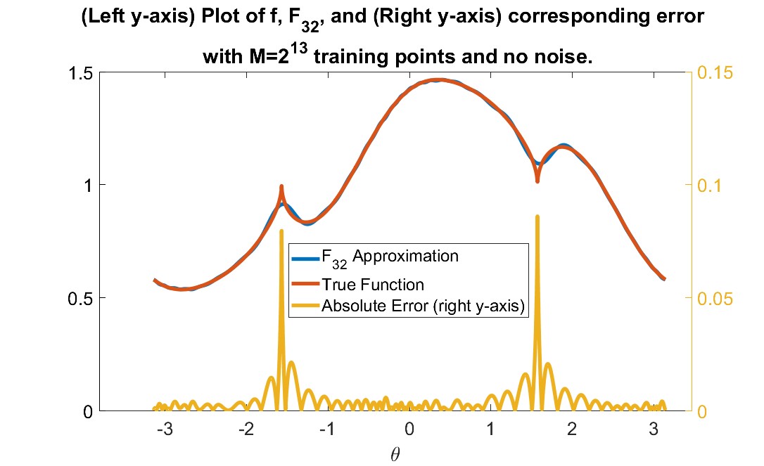
In this section, we illustrate our theory with some numerical experiments. In Section 4.1, we consider the approximation of a piecewise differentiable function, and demonstrate how the localization of the kernel leads to a determination of the locations of the singularities. The example in Section 4.2 is motivated by magnetic resonance relaxomety. In both examples, we will examine how the accuracy of the approximation depends on the degree $<n$ of the polynomial, the number $M$ of samples, and the level of noise.

4.1 Piecewise differentiable function

In this example only we define the function to be approximated as

$$f(\theta)\coloneqq 1+\left|\cos\theta\right|^{1/2}\sin(\cos\theta+\sin\theta)/2,$$ (4.1)

defined on the ellipse

$$E=\{(3\cos\theta,6\sin\theta):\theta\in[0,2\pi)\}.$$ (4.2)

We project $E$ to the sphere $\mathbb{S}^{2}$ using an inverse stereographic projection defined by

$$\mathbf{P}(\mathbf{x})=\frac{(\mathbf{x},1)}{\left|\left|(\mathbf{x},1)\right|\right|_{2}},$$ (4.3)

and call $\mathbb{X}=\mathbf{P}(E)$. We simply correspond each $\mathbf{x}\in\mathbb{X}$ with the value $\theta_{\mathbf{x}}$ satisfying $\mathbf{x}=\mathbf{P}\big{(}(3\cos\theta_{\mathbf{x}},6\sin\theta_{\mathbf{x}})\big{)}$, so that $f(\mathbf{x})\coloneqq f(\theta_{\mathbf{x}})$ is a continuous function on $\mathbb{X}$.

We generate our data points by taking $\mathbf{y}_{j}=\mathbf{P}\big{(}(3\cos\theta_{j},6\sin\theta_{j})\big{)}$, where $\theta_{j}$ are each sampled uniformly from $[0,2\pi]$. We then define $z_{j}=f(\mathbf{y}_{j})+\epsilon_{j}$ where $\epsilon_{j}$ are sampled from some mean-zero normal noise. Our data set is thus $\mathcal{D}\coloneqq\{(\mathbf{y}_{j},f(\mathbf{y}_{j})+\epsilon_{j})\}_{j=1}^{M}$. We will measure the magnitude of noise using the signal to noise ratio (SNR), defined by

$$20\log_{10}\Big{(}\left|\left|\big{(}f(\mathbf{y}_{1}),\dots,f(\mathbf{y}_{M})\big{)}\right|\right|_{2}\Big{/}\left|\left|\big{(}\epsilon_{1},\dots,\epsilon_{M}\big{)}\right|\right|_{2}\Big{)}.$$ (4.4)

Since $f_{0}\neq 1$ in this case, we could calculate $f_{0}$ from the projection or we may estimate it using Corollary 3.2. That is,

$$f_{0}(\mathbf{x})\approx\frac{1}{M}\sum_{j=1}^{M}\Phi_{n,1}(\mathbf{x}\cdot\mathbf{y}_{j}).$$ (4.5)

This option may be desirable in cases where $f_{0}$ is not feasible to compute (i.e. if the underlying domain of the data is unknown or irregularly shaped). Our approximation is thus:

$$F_{n}(\mathbf{x})=\sum_{j=1}^{M}(f(\mathbf{y}_{j})+\epsilon_{j})\Phi_{n,1}(\mathbf{x}\cdot\mathbf{y}_{j})\left/\left(\sum_{j=1}^{M}\Phi_{n,1}(\mathbf{x}\cdot\mathbf{y}_{j})\right).\right.$$ (4.6)
Refer to caption
Figure 1: Left y-axis: Plot of the true function $f$ compared with $F_{32}$ constructed by $2^{13}$ noiseless training points. Right y-axis: Plot of $\left|f-F_{32}\right|$.
Refer to caption Refer to caption Refer to caption
Figure 2: (Left) Plot of sorted $\log_{10}|F_{n}-f|$ error values for various choices of $n$ with $M=2^{13}$ training points and no noise. (Center) Plot of sorted $\log_{10}|F_{64}-f|$ error values for various choices of $M$ with no noise. (Right) Plot of sorted $\log_{10}|F_{64}-f|$ error values for various noise levels with $M=2^{13}$ training points.

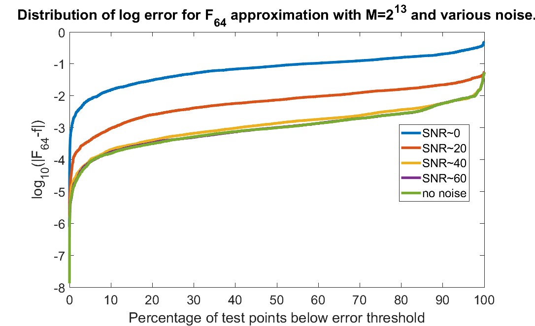
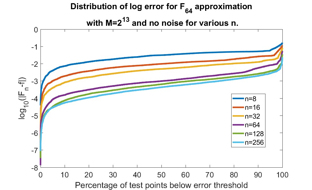
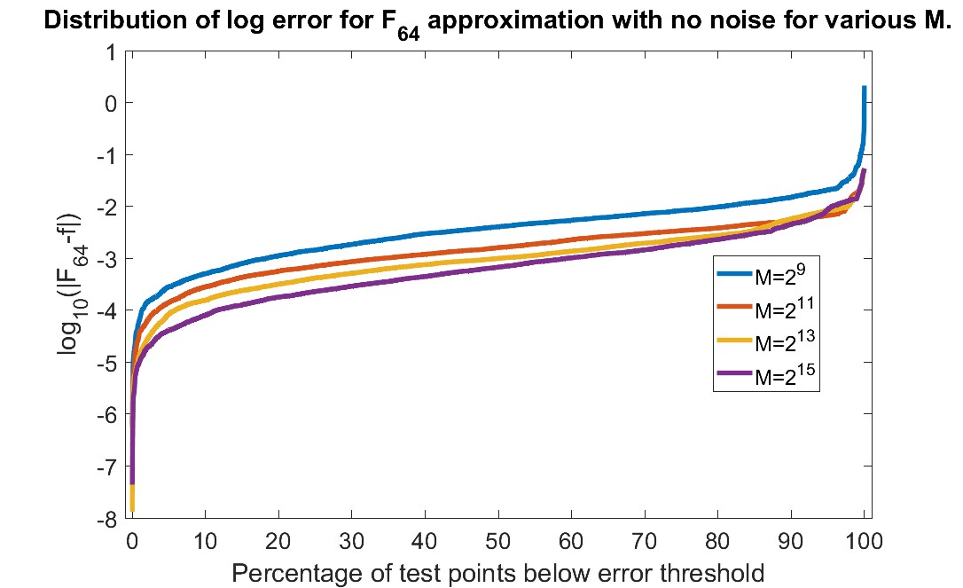
Figure 1 demonstrates that the approximation does much better than the uniform error bound when the function is relatively smooth, and the error only spikes locally where the derivative of $f$ is undefined, i.e $\theta=\pm\pi/2$. Figure 2 displays three graphs illustrating how the distribution of $\log_{10}|F_{n}-f|$ behaves for various choices of $n,M,\epsilon$. The first graph shows the trend for various $n$ values. As we increase $n$, we see consistent drop in error across the span of the domain. The second graph shows various values of $M$. We again see a decrease in the overall error as $M$ is increased. The third graph shows how the log error decreases as the noise decreases. We can see that the approximation is much worse for low SNR values, but nearly indistinguishable from the noiseless case when the SNR is above 60.

4.2 Parameter estimation in bi-exponential sums

This example is motivated by magnetic resonance relaxometry, in which the proton nuclei of water are first excited with radio frequency pulses and then exhibit an exponentially decaying electromagnetic signal. When one may assume the presence of two water compartments undergoing slow exchange, with signal corrupted by additive Gaussian noise, the signal is modeled typically as a bi-exponential decay function (4.7) (cf. [31]):

$$F(t)=c_{1}\exp(-t/T_{2,1})+c_{2}\exp(-t/T_{2,2})+E(t),$$

where $E$ is the noise, and $T_{2,1},T_{2,2}>0$, and the time $t$ is typically sampled at equal intervals. Writing $t=j\delta$, $\lambda_{1}=\delta/T_{2,1}$, $\lambda_{2}=\delta/T_{2,2}$, we may reformulate the data as

$$f(j)\coloneqq f(\lambda_{1},\lambda_{2},j)=c_{1}e^{-\lambda_{1}j}+c_{2}e^{-\lambda_{2}j}+\epsilon(j),$$ (4.7)

where $\epsilon(j)$ are samples of mean-zero normal noise.

In this example, we consider the case where $c_{1}=.7,c_{2}=.3$ and use our method to determine the values $\lambda_{1},\lambda_{2}$, given data of the form

$$\tilde{\mathbf{y}}(\lambda_{1},\lambda_{2})\coloneqq(f(1),f(2),\dots,f(100)).$$ (4.8)

We “train” our approximation process with $M$ samples of $(\lambda_{1,j},\lambda_{2,j})\in[.1,.7]\times[1.1,1.7]$ chosen uniformly at random and then plugging those values into (4.7) to generate vectors of the form shown in (4.8). The dimension of the input data is $Q=100$, however (in the noiseless case) the data lies on a $q=2$ dimensional manifold, so we will use $\Phi_{n,2}$ to generate our approximations. In the noisy case, this problem does not perfectly fit the theory studied in this paper since the noise is applied to the input values $f(t)$ meaning we cannot assume they lie directly on an unknown manifold anymore. Nevertheless we can see some success with our method. We define the operators

$$\mathbf{T}(\tilde{\mathbf{y}})=1000\tilde{\mathbf{y}}-(380,189,116,0,\dots,0),\qquad\mathbf{P}(\circ)=\frac{(\circ,100)}{\left|\left|(\circ,100)\right|\right|_{2}}$$ (4.9)

and denote $\mathbf{y}=\mathbf{P}(\mathbf{T}(\tilde{\mathbf{y}}))$. In practice one can imagine the choice of these operators to be a hyper-parameter of the model. We use the same density estimation as in Section 4.1:

$$\operatorname{DE}\big{(}\mathbf{x}(\lambda_{1},\lambda_{2})\big{)}=\sum_{j=1}^{M}\Phi_{n,2}\big{(}\mathbf{x}(\lambda_{1},\lambda_{2})\cdot\mathbf{y}(\lambda_{1,j},\lambda_{2,j})\big{)}.$$ (4.10)

As a result, our approximation process looks like:

$$\begin{bmatrix}\lambda_{1}\\ \lambda_{2}\end{bmatrix}\approx\mathbf{F}_{n}\big{(}\mathbf{x}(\lambda_{1},\lambda_{2})\big{)}=\sum_{j=1}^{M}\begin{bmatrix}\lambda_{1,j}\\ \lambda_{2,j}\end{bmatrix}\Phi_{n,2}\big{(}\mathbf{x}(\lambda_{1},\lambda_{2})\cdot\mathbf{y}(\lambda_{1,j},\lambda_{2,j})\big{)}\Big{/}\operatorname{DE}\big{(}\mathbf{x}(\lambda_{1},\lambda_{2})\big{)}.$$ (4.11)

Similar to Example 4.1, we will include figures showing how results are effected as $n,M,\epsilon$ are adjusted. We measure noise using the signal to noise ration (SNR) defined by

$$20\log_{10}\left(\left|\left|\tilde{\mathbf{y}}\right|\right|_{2}\Big{/}\left|\left|\big{(}\epsilon(1),\dots,\epsilon(100)\big{)}\right|\right|_{2}\right).$$ (4.12)

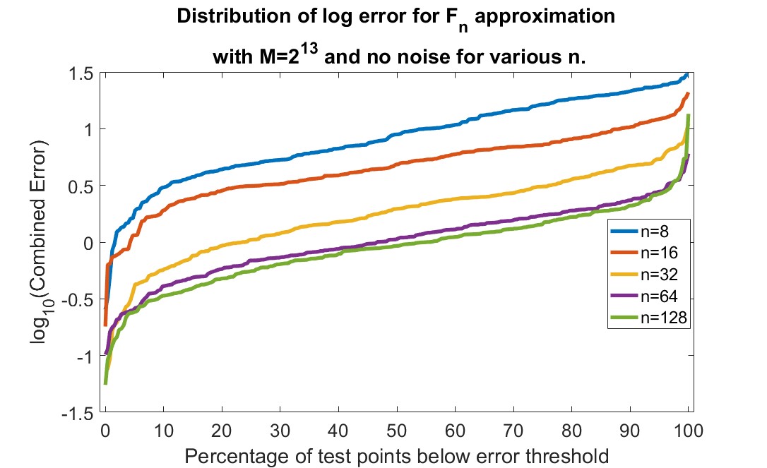
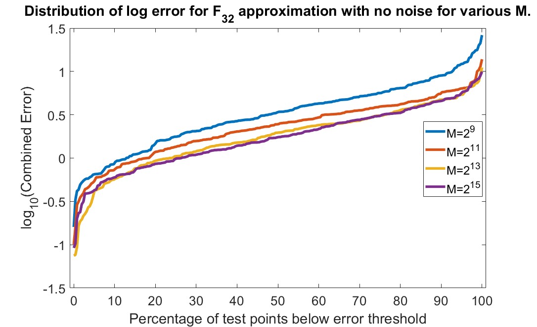
Unlike Example 4.1, we will now be considering percent approximation error instead of uniform error as it is more relevant in this problem. We define the combined error to be

$$100*\sum_{j=1}^{2}\frac{\left|\lambda_{j,\text{true}}-\lambda_{j,\text{approx}}\right|}{\lambda_{j,\text{true}}}.$$ (4.13)
Refer to caption Refer to caption Refer to caption
Figure 3: (Left) Plot of sorted log combined error values for various choices of $n$, fixed $M=2^{13}$ training points, and no noise. (Center) Plot of sorted log combined error values for fixed $n=32$, various choices of $M$, and no noise. (Right) Plot of sorted log combined error values for fixed $n=32$, fixed $M=2^{13}$ training points, and various noise levels.

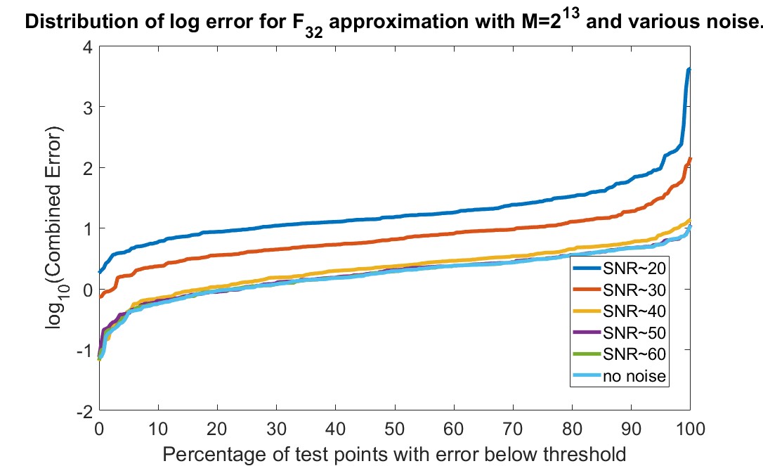
Figure 3 depicts three graphs showing the distribution of sorted $\log_{10}$(Combined Error) points for various $n,M,\epsilon$. In the first graph, we see the distribution of for various choices of $n$. As $n$ increases, the overall error decreases. An interesting phenomenon occurring in this figure is with the $n=128$ case where the uniform error is actually higher than the $n=64$ case. This is likely due to the fact that overfitting might occur if $n$ gets too large for fixed $M$. The second graph illustrates how the approximation improves as $M$ is increased. While the decrease in error is not uniform, we do see an overall trend of decreasing error as $M$ increases. In the third graph, we see that the approximation improves as the noise decreases. There is very little noticeable difference between the noiseless case and any case where SNR$>50$.

5 Proofs

The purpose of this section is to prove Theorem 3.1. We can think of $F_{n}(\mathcal{D},x)$ defined in (3.5) as an empirical approximation for an expected value with respect to $\tau$:

$$\mathbb{E}_{\tau}(F_{n}(\mathcal{D},x))=\int z\Phi_{n,q}(x\cdot y)d\tau(y)=\int_{\mathbb{X}}f(y)\Phi_{n,q}(x\cdot y)f_{0}(y)d\mu^{*}(y).$$ (5.1)

Accordingly, we define an integral reconstruction operator by

$$\sigma_{n}(\mathbb{X},f)(x)\coloneqq\int_{\mathbb{X}}\Phi_{n,q}(x\cdot y)f(y)d\mu^{*}(y),\qquad f\in C(\mathbb{X}),\ x\in\mathbb{X}.$$ (5.2)

In Section 5.1, we study the approximation properties of this operator (Theorem 5.1). In Secion 5.2, we use this theorem with $f_{0}f$ in place of $f$, and use the Bernstein concentration inequality (Proposition 5.1) to discretize the integral expression in (5.2) and complete the proof of Theorem 3.1.

5.1 Integral reconstruction operator

In this section, we prove the following theorem which is an integral analogue of Theorem 3.1.

Theorem 5.1.

Let $0<\gamma<2$, $f\in W_{\gamma}(\mathbb{X})$. Then for $n\geq 1$, we have

$$\left|\left|f-\sigma_{n}(\mathbb{X},f)\right|\right|_{\mathbb{\mathbb{X}}}\lesssim n^{-\gamma}\left|\left|f\right|\right|_{W_{\gamma}(\mathbb{X})}.$$ (5.3)

In order to prove this theorem, we will use a covering of $\mathbb{X}$ using balls of radius $\iota^{*}$, and a corresponding partition of unity. A key lemma to facilitate the details here is the following.

Lemma 5.1.

Let $x\in\mathbb{X}$. Let $g\in C(\mathbb{X})$ be supported on $\mathbb{B}(x,\iota^{*})$. If $G(u)=g(\eta_{x}(u))$, $0<\gamma<2$. Then

$$\left|\int_{\mathbb{X}}\Phi_{n,q}(x\cdot y)g(y)d\mu^{*}(y)-\int_{\mathbb{S}_{x}(\mathbb{X})}\Phi_{n,q}(x\cdot u)G(u)d\mu_{q}^{*}(u)\right|\leq cn^{-\gamma}||g||_{\mathbb{X}}.$$ (5.4)

Naturally, the first step in this proof is to show that the Lebesgue constant for the kernel $\Phi_{n,q}$ is bounded independently of $n$. This is done in the following lemma.

Lemma 5.2.

Let $r>0$ and $n\geq 1/r$. If $\Phi_{n,q}$ is given as in (2.12) with $S>q$, then

$$\sup_{x\in\mathbb{X}}\int_{\mathbb{X}\setminus\mathbb{B}(x,r)}\left|\Phi_{n,q}(x\cdot y)\right|d\mu^{*}(y)\lesssim\max(1,nr)^{q-S}.$$ (5.5)

Additionally,

$$\sup_{x\in\mathbb{X}}\int_{\mathbb{X}}|\Phi_{n,q}(x\cdot y)|d\mu^{*}(y)\lesssim 1.$$ (5.6)
Proof.

Recall from Proposition A.2 that $\rho(x,y)\sim\arccos(x\cdot y)$, so (2.13) implies

$$\left|\Phi_{n,q}(x\cdot y)\right|\lesssim\frac{n^{q}}{\max(1,n\arccos(x\cdot y))^{S}}\lesssim\frac{n^{q}}{\max(1,n\rho(x,y))^{S}}.$$ (5.7)

In this proof only, we fix $x\in\mathbb{X}$. Let $A_{0}=\mathbb{B}(x,r)$ and $A_{k}=\mathbb{B}(x,2^{k}r)\setminus\mathbb{B}(x,2^{k-1}r)$. Then $\mu^{*}(A_{k})\lesssim 2^{k}qr^{q}$, and for any $y\in A_{k}$, $2^{k-1}r\leq\rho(x,y)\leq 2^{k}r$.

First, let $nr\geq 1$. In view of (3.3) and (5.7), it follows that

$\displaystyle\int_{\mathbb{X}\setminus\mathbb{B}(x,r)}\left|\Phi_{n,q}(x\cdot y)\right|d\mu^{*}(y)=$ $\displaystyle\sum_{k=1}^{\infty}\int_{A_{k}}\left|\Phi_{n,q}(x\cdot y)\right|d\mu^{*}(y)\lesssim\sum_{k=1}^{\infty}\frac{\mu^{*}(A_{k})n^{q}}{(n2^{k-1}r)^{S}}$ (5.8)
$\displaystyle\lesssim$ $\displaystyle(nr)^{q-S}\sum_{k=0}^{\infty}2^{k(q-S)}\leq(nr)^{q-S}.$

Using this estimate with $r=1/n$ and the condition (3.3) on the measures of balls we see that

$$\int_{\mathbb{X}}\left|\Phi_{n,q}(x\cdot y)\right|d\mu^{*}(y)=\int_{A_{0}}\left|\Phi_{n,q}(x\cdot y)\right|d\mu^{*}(y)+\int_{\mathbb{X}\setminus\mathbb{B}(x,r)}\left|\Phi_{n,q}(x\cdot y)\right|d\mu^{*}(y)\lesssim(nr)^{q}+(nr)^{q-S}\sim 1.$$

Since the choice of $x$ was arbitrary, we have proven (5.6). Then (5.6) and (5.8) combined give the bounds for (5.5). ∎

Next, we prove Lemma 5.1.

Proof of Lemma 5.1.

Since $\gamma<2$, we may choose (for sufficiently large $n$)

$$\delta=n^{-(\gamma+q+1)/(q+3)},\quad n\delta=n^{(2-\gamma)/(q+3)}>1,\quad S>\frac{2q+3\gamma}{2-\gamma}.$$ (5.9)

We may assume further that $\delta<\iota^{*}$. Then, by using (2.14) and Proposition A.2, we have for any $u\in\mathbb{S}_{x}(\delta)$,

$\displaystyle\biggl{|}\Phi_{n,q}(x\cdot\eta_{x}(u))$ $\displaystyle-\Phi_{n,q}(x\cdot u)\biggr{|}\lesssim n^{q+1}\left|\arccos(x\cdot\eta_{x}(u))-\arccos(x\cdot u)\right|$ (5.10)
$\displaystyle=$ $\displaystyle n^{q+1}\left|\arccos(x\cdot\eta_{x}(u))-\rho(x\cdot\eta_{x}(u))\right|\lesssim n^{q+1}\rho(x,\eta_{x}(u))^{3}\lesssim n^{q+1}\delta^{3}.$

Letting $g_{1},g_{2}$ be the metric tensors associated with the maps $\varepsilon_{x},\overline{\varepsilon}_{x}$ respectively, then we have the following change of variables formulas (cf. Table 1):

$$\int_{\mathbb{B}(x,\delta)}d\mu^{*}(\varepsilon_{x}(v))=\int_{B_{\mathbb{T}}(x,\delta)}\sqrt{|g_{1}|}dv,\qquad\int_{\mathbb{S}_{x}(\delta)}d\mu^{*}_{q}(u)=\int_{B_{\mathbb{T}}(x,\delta)}\sqrt{|g_{2}|}d\overline{\varepsilon}^{-1}_{x}(u).$$ (5.11)

We set $v=\overline{\varepsilon}^{-1}_{x}(u)$ and use fact (cf. (A.10)) that on $B_{\mathbb{T}}(x,\delta)$, $\sqrt{|g_{1}|}-1\lesssim\delta^{2}$ and $\sqrt{|g_{2}|}-1\lesssim\delta^{2}$. Then by applying Equations (5.10), (5.11) (2.13), and (2.14), we can deduce

$\displaystyle\Biggl{|}\int_{\mathbb{B}(x,\delta)}\Phi_{n,q}(x\cdot y)$ $\displaystyle g(y)d\mu^{*}(y)-\int_{\mathbb{S}_{x}(\delta)}\Phi_{n,q}(x\cdot u)G(u)d\mu^{*}_{\mathbb{S}_{x}}(u)\Biggr{|}$ (5.12)
$\displaystyle\leq$ $\displaystyle\left|\int_{B_{\mathbb{T}}(x,\delta)}\Phi_{n,q}(x\cdot\varepsilon_{x}(v))g(\varepsilon_{x}(v))(\sqrt{|g_{1}|}-\sqrt{|g_{2}|})dv\right|$
$\displaystyle\qquad+\left|\int_{\mathbb{S}_{x}(\delta)}(\Phi_{n,q}(x\cdot\eta_{x}(u))-\Phi_{n,q}(x\cdot u))G(u)d\mu^{*}_{\mathbb{S}_{x}}(u)\right|$
$\displaystyle\lesssim$ $\displaystyle\left|\left|g\right|\right|_{\mathbb{X}}(\delta^{q+2}n^{q}+\delta^{q+3}n^{q+1})\leq\delta^{q+3}n^{q+1}\left|\left|g\right|\right|_{\mathbb{X}}(1/(n\delta)+1)\lesssim\left|\left|g\right|\right|_{\mathbb{X}}n^{-\gamma}.$

Now it only remains to examine the terms away from $\mathbb{S}_{x}(\delta),\mathbb{B}(x,\delta)$. Utilizing Lemma 5.2, and the fact that $S\geq\frac{2q+3\gamma}{2-\gamma}$, we have

$$\left|\int_{\mathbb{X}\setminus\mathbb{B}(x,\delta)}\Phi_{n,q}(x\cdot y)g(y)d\mu^{*}(y)\right|\lesssim\left|\left|g\right|\right|_{\mathbb{X}}(n\delta)^{q-S}=\left|\left|g\right|\right|_{\mathbb{X}}n^{(q-S)(2-\gamma)/(q+3)}\lesssim\left|\left|g\right|\right|_{\mathbb{X}}n^{-\gamma}.$$ (5.13)

Similarly, again using Lemma 5.2 (with $\mathbb{S}_{x}$ as the manifold) and observing $\left|\left|g\right|\right|_{\mathbb{X}}=\left|\left|G\right|\right|_{\mathbb{S}_{x}}$, we can conclude

$$\left|\int_{\mathbb{S}_{x}\setminus\mathbb{S}_{x}(\delta)}\Phi_{n,q}(x\cdot u)G(u)d\mu_{\mathbb{S}_{x}}^{*}(u)\right|\lesssim\left|\left|G\right|\right|_{\mathbb{S}_{x}}(n\delta)^{q-S}\lesssim\left|\left|g\right|\right|_{\mathbb{X}}n^{-\gamma},$$ (5.14)

completing the proof. ∎

We are now in a position to complete the proof of Theorem 5.1.

Proof of Theorem 5.1.

Let $x\in\mathbb{X}$. Choose $\phi\in C^{\infty}$ such that $0\leq\phi(y)\leq 1$ for all $y\in\mathbb{X}$, $\phi(y)=1$ on $\mathbb{B}(x,\iota^{*}/2)$, and $\phi(y)=0$ on $\mathbb{X}\backslash\mathbb{B}(x,\iota^{*})$. Then $f\phi$ is supported on $\mathbb{B}(x,\iota^{*})$ and $F(u)\coloneqq\phi(\eta_{x}(u))f(\eta_{x}(u))$ belongs to $W_{\gamma}(\mathbb{S}_{x})$. We observe $\left|\left|f\right|\right|_{\mathbb{X}}\lesssim\left|\left|f\right|\right|_{W_{\gamma}(\mathbb{X})}$. By Lemma 5.2,

$$\left|\int_{\mathbb{X}}\Phi_{n,q}(x\cdot y)f(y)(1-\phi(y))d\mu^{*}(y)\right|\leq\left|\left|f\right|\right|_{\mathbb{X}}\int_{\mathbb{X}\setminus\mathbb{B}(x,\iota^{*}/2)}\left|\Phi_{n,q}(x\cdot y)\right|d\mu^{*}(y)\lesssim n^{-\gamma}\left|\left|f\right|\right|_{W_{\gamma}(\mathbb{X})}.$$ (5.15)

Note that the constant above is chosen to account for the case where $n<2/\iota^{*}$. By Lemma 5.1,

$$\left|\int_{\mathbb{X}}\Phi_{n,q}(x\cdot y)f(y)\phi(y)d\mu^{*}(y)-\sigma_{n}(\mathbb{S}_{x},F)(x)\right|\lesssim n^{-\gamma}\left|\left|f\phi\right|\right|_{\mathbb{X}}\lesssim n^{-\gamma}\left|\left|f\right|\right|_{W_{\gamma}(\mathbb{X})}.$$ (5.16)

Observe that since $f(x)=F(x)$ and $\left|\left|F\right|\right|_{W_{\gamma}(\mathbb{S}_{x})}\leq\left|\left|f\right|\right|_{W_{\gamma}(\mathbb{X})}$,

$\displaystyle|f(x)$ $\displaystyle-\sigma_{n}(\mathbb{X},f)(x)|$ (5.17)
$\displaystyle\leq|f(x)-F(x)|+|F(x)-\sigma_{n}(\mathbb{S}_{x},F)(x)|+|\sigma_{n}(\mathbb{S}_{x},F)(x)-\sigma_{n}(\mathbb{X},f)(x)|$
$\displaystyle\lesssim 0+\left|\sigma_{n}(\mathbb{S}_{x},F)(x)-\int_{\mathbb{X}}\Phi_{n,q}(x\cdot y)f(y)\phi(y)d\mu^{*}(y)\right|+\left|\int_{\mathbb{X}}\Phi_{n,q}(x\cdot y)f(y)(1-\phi(y))d\mu^{*}(y)\right|$
$\displaystyle\leq n^{-\gamma}\left|\left|f\right|\right|_{W_{\gamma}(\mathbb{X})}.$

Since this bound is independent of $x$, the proof is completed. ∎

5.2 Discretization

In order to complete the proof of Theorem 3.1, we need to discretize the integral operator in Theorem 5.1 while keeping track of the error. If the manifold were known and we could use the eigen-decomposition of the Laplace-Beltrami operator, we could do this discretization without losing the accuracy using quadrature formulas (cf., e.g., [15]). In our current set up, it is more natural to use concentration inequalities. We will use the inequality summarized in Proposition 5.1 below (c.f. [32]).

Proposition 5.1 (Bernstein concentration inequality).

Let $Z_{1},\cdots,Z_{M}$ be independent real valued random variables such that for each $j=1,\dots,M$, $|Z_{j}|\leq R$, and $\mathbb{E}(Z_{j}^{2})\leq V$. Then for any $t>0$,

$$\operatorname{Prob}\left(\left|\frac{1}{M}\sum_{j=1}^{M}(Z_{j}-\mathbb{E}(Z_{j}))\right|\geq t\right)\leq 2\exp\left(-\frac{Mt^{2}}{2(V+Rt/3)}\right).$$ (5.18)

In the following, we will set $Z_{j}(x)=z_{j}\Phi_{n,q}(x\cdot y_{j})$, where $(y_{j},z_{j})$ are sampled from $\tau$. The following lemma estimates the variance of $Z_{j}$.

Lemma 5.3.

With the setup from Theorem 3.1, we have

$$\sup_{x\in\mathbb{X}}\int\left|z\Phi_{n,q}(x\cdot y)\right|^{2}d\tau(y,z)\lesssim n^{q}\left|\left|z\right|\right|^{2}_{\infty}\left|\left|f_{0}\right|\right|_{\mathbb{X}},\qquad x\in\SS^{Q}.$$ (5.19)
Proof.

We observe that (2.13) and Lemma 5.2 imply that

$$\sup_{x\in\mathbb{X}}\int_{\mathbb{X}}\Phi_{n,q}(x\cdot y)^{2}d\mu^{*}(y)\lesssim n^{q}\sup_{x\in\mathbb{X}}\int_{\mathbb{X}}\left|\Phi_{n,q}(x\cdot y)\right|d\mu^{*}(y)\lesssim n^{q}.$$ (5.20)

Hence,

$$\sup_{x\in\mathbb{X}}\int\left|z(y,\epsilon)\Phi_{n,q}(x\cdot y)\right|^{2}d\tau(y,z)\leq\left|\left|z\right|\right|^{2}_{\infty}\left|\left|f_{0}\right|\right|_{\mathbb{X}}\sup_{x\in\mathbb{X}}\int_{\mathbb{X}}\Phi_{n,q}(x\cdot y)^{2}d\mu^{*}(y)\lesssim n^{q}\left|\left|z\right|\right|^{2}_{\infty}\left|\left|f_{0}\right|\right|_{\mathbb{X}}.$$ (5.21)

A limitation of the Bernstein concentration inequality is that it only considers a single $x$ value. Since we are interested in supremum-norm bounds, we must first relate the supremum-norm of $Z_{j}$ over all $x\in\mathbb{S}^{Q}$ to a finite set of points. We set up the connection in the following lemma.

Lemma 5.4.

Let $\nu$ be any (bounded variation) measure on $\mathbb{X}$. Then there exists a finite set $\mathcal{C}$ of size $|\mathcal{C}|\sim n^{Q}$ such that

$$\left|\left|\int_{\mathbb{X}}\Phi_{n,q}(\circ\cdot y)d\nu(y)\right|\right|_{\mathbb{S}^{Q}}\leq 2\max_{x\in\mathcal{C}}\left|\int_{\mathbb{X}}\Phi_{n,q}(x\cdot y)d\nu(y)\right|.$$ (5.22)
Proof.

In view of the Bernstein inequality for the derivatives of spherical polynomials, we see that

$$\left|P(x)-P(y)\right|\leq cn\left|\left|x-y\right|\right|_{\infty}\left|\left|P\right|\right|_{\infty},\qquad P\in\Pi_{n}^{Q}.$$ (5.23)

We can see by construction that $\int_{\mathbb{X}}\Phi_{n,q}(t,y)d\nu(y)$ is a polynomial of degree $<n$ in the variable $t$. Since $\mathbb{S}^{Q}$ is a compact space and polynomials of degree $<n$ are continuous functions, there exists some $x^{*}\in\mathbb{S}^{Q}$ such that

$$\left|\left|\int_{\mathbb{X}}\Phi_{n,q}(\circ\cdot y)d\nu(y)\right|\right|_{\infty}=\left|\int_{\mathbb{X}}\Phi_{n,q}(x^{*}\cdot y)d\nu(y)\right|.$$ (5.24)

Let $c$ be the same as in (5.23) and $\mathcal{C}$ be a finite set satisfying

$$\max_{x\in\mathbb{S}^{Q}}\min_{y\in\mathcal{C}}\left|\left|x-y\right|\right|_{\infty}\leq\frac{1}{2cn}.$$ (5.25)

Since $\mathbb{S}^{Q}$ is a compact $Q$-dimensional space, the set $\mathcal{C}$ needs no more than $\sim n^{Q}$ points.

Then there exists some $z^{*}\in\mathcal{C}$ such that

$$\left|\int_{\mathbb{X}}(\Phi_{n,q}(x^{*}\cdot y)-\Phi_{n,q}(z^{*}\cdot y))d\nu(y)\right|\lesssim n\left|\left|x^{*}-z^{*}\right|\right|_{\infty}\left|\int_{\mathbb{X}}\Phi_{n,q}(x^{*}\cdot y)d\nu(y)\right|,$$ (5.26)

which implies (5.22).

With this preparation, we now give the following theorem.

Theorem 5.2.

Assume the setup of Theorem 3.1. Then for every $n\geq 1$ and $M\gtrsim n^{q+2\gamma}\log(n/\delta)$ we have

$$\operatorname{Prob}_{\tau}\left(\left|\left|F_{n}(\mathcal{D},\circ)-\sigma_{n}(\mathbb{X},ff_{0})\right|\right|_{\mathbb{S}^{Q}}\geq c\left|\left|z\right|\right|_{\infty}n^{-\gamma}\sqrt{\left|\left|f_{0}\right|\right|_{\mathbb{X}}}\right)\leq\delta.$$ (5.27)
Proof.

In this proof only, constants $c,c_{1},c_{2},\dots$ will maintain their value once used. Let $Z_{j}(x)=z_{j}\Phi_{n,q}(x\cdot y_{j})$. Since $z$ is integrable with respect to $\tau$, one has the following for any $x\in\mathbb{S}^{Q}$:

$$\mathbb{E}_{\tau}(Z_{j}(x))=\int_{\mathbb{X}}\mathbb{E}_{\tau}(z|y)\Phi_{n,q}(x\cdot y)d\nu^{*}(y)=\int_{\mathbb{X}}f(y)\Phi_{n,q}(x\cdot y)f_{0}(y)d\mu^{*}(y)=\sigma_{n}(\mathbb{X},ff_{0})(x).$$ (5.28)

We have from (2.13) that $\left|Z_{j}\right|\lesssim n^{q}\left|\left|z\right|\right|_{\infty}$. Lemma 5.3 informs us that $\mathbb{E}_{\tau}(Z_{j}^{2})\lesssim n^{q}\left|\left|z\right|\right|_{\infty}^{2}\left|\left|f_{0}\right|\right|_{\mathbb{X}}$. Assume $0<r\leq 1$ and set $t=r\left|\left|z\right|\right|_{\infty}\left|\left|f_{0}\right|\right|_{\mathbb{X}}$. From Proposition 5.1, we see

$\displaystyle\operatorname{Prob}_{\tau}\left(\left|\frac{1}{M}\sum_{j=1}^{M}Z_{j}(x)-\sigma_{n}(\mathbb{X},ff_{0})(x)\right|\geq t\right)\leq$ $\displaystyle 2\exp\left(-c_{1}\frac{Mt^{2}}{(n^{q}\left|\left|z\right|\right|_{\infty}^{2}\left|\left|f_{0}\right|\right|_{\mathbb{X}}+n^{q}\left|\left|z\right|\right|_{\infty}t/3)}\right)$ (5.29)
$\displaystyle\leq$ $\displaystyle 2\exp\left(-c_{2}\frac{M\left|\left|f_{0}\right|\right|_{\mathbb{X}}r^{2}}{n^{q}}\right).$

Let $\delta\in(0,1/2)$, $\mathcal{C}$ be a finite set satisfying (5.25) with $\left|\mathcal{C}\right|\leq c_{3}n^{Q}$ (without loss of generality we assume $c_{3}\geq 1$),

$$c_{4}\geq\frac{\max\big{(}\log_{2}(c_{3})+1,Q\big{)}}{c_{2}},$$ (5.30)

and

$$M\geq c_{4}n^{q+2\gamma}\log(n/\delta).$$ (5.31)

We now fix

$$r\equiv\sqrt{c_{4}\frac{n^{q}}{M\left|\left|f_{0}\right|\right|_{\mathbb{X}}}\log(n/\delta)}.$$ (5.32)

Notice that since $\left|\left|f_{0}\right|\right|_{\mathbb{X}}\geq 1$, our assumption of $M$ in (5.31) implies

$$r\leq n^{-\gamma}\big{/}\sqrt{\left|\left|f_{0}\right|\right|_{\mathbb{X}}}\leq 1,$$ (5.33)

so our choice of $r$ does in fact satisfy (5.29). Further,

$$r\left|\left|z\right|\right|_{\infty}\left|\left|f_{0}\right|\right|_{\mathbb{X}}\leq c\left|\left|z\right|\right|_{\infty}n^{-\gamma}\sqrt{\left|\left|f_{0}\right|\right|_{\mathbb{X}}}.$$ (5.34)

With this preparation, we can conclude

$\displaystyle\operatorname{Prob}_{\tau}\bigg{(}\big{\|}F_{n}(\mathcal{D};\circ)$ $\displaystyle-\sigma_{n}(\mathbb{X},ff_{0})\big{\|}_{\mathbb{S}^{Q}}\geq c\left|\left|z\right|\right|_{\infty}n^{-\gamma}\sqrt{\left|\left|f_{0}\right|\right|_{\mathbb{X}}}\bigg{)}$ (5.35)
$\displaystyle\leq$ $\displaystyle\operatorname{Prob}_{\tau}\left(\left|\left|\frac{1}{M}\sum_{j=1}^{M}Z_{j}-\sigma_{n}(\mathbb{X},ff_{0})\right|\right|_{\mathbb{S}^{Q}}\geq r\left|\left|z\right|\right|_{\infty}\left|\left|f_{0}\right|\right|_{\mathbb{X}}\right)$ (from (5.34))
$\displaystyle\leq$ $\displaystyle\operatorname{Prob}_{\tau}\left(\max_{x_{k}\in\mathcal{C}}\left(\left|\frac{1}{M}\sum_{j=1}^{M}Z_{j}(x_{k})-\sigma_{n}(\mathbb{X},ff_{0})(x_{k})\right|\right)\geq t\right)$ (by Lemma 5.4)
$\displaystyle\leq$ $\displaystyle\sum_{k=1}^{\left|\mathcal{C}\right|}\operatorname{Prob}_{\tau}\left(\left|\frac{1}{M}\sum_{j=1}^{M}Z_{j}(x_{k})-\sigma_{n}(\mathbb{X},ff_{0})(x_{k})\right|\geq t\right)$
$\displaystyle\leq$ $\displaystyle|\mathcal{C}|\exp\left(-c_{2}\frac{M\left|\left|f_{0}\right|\right|_{\mathbb{X}}r^{2}}{n^{q}}\right)$ (from (5.29))
$\displaystyle\leq$ $\displaystyle c_{3}n^{Q-c_{2}c_{4}}\delta^{c_{2}c_{4}}$ (from (5.32))
$\displaystyle\leq$ $\displaystyle c_{3}n^{Q-Q}\left(\frac{1}{2}\right)^{\log_{1/2}(1/c_{3})}\delta$ (from (5.30) and $\delta<1/2$)
$\displaystyle\leq$ $\displaystyle\delta.$

We are now ready for the proof of Theorem 3.1.

Proof of Theorem 3.1 (and Corollary 3.1 and 3.2)..

Since $f,f_{0}\in W_{\gamma}(\mathbb{X})$, we can determine that $ff_{0}\in W_{\gamma}(\mathbb{X})$ as well. Utilizing Theorem 5.1 with $ff_{0}$ and Theorem 5.2, we obtain with probability at least $1-\delta$ that

$\displaystyle\left|\left|F_{n}(\mathcal{D};\circ)-ff_{0}\right|\right|_{\mathbb{X}}\leq$ $\displaystyle\left|\left|F_{n}(\mathcal{D};\circ)-\sigma_{n}(\mathbb{X};ff_{0})\right|\right|_{\mathbb{X}}+\left|\left|\sigma_{n}(\mathbb{X};ff_{0})-ff_{0}\right|\right|_{\mathbb{X}}$ (5.36)
$\displaystyle\lesssim$ $\displaystyle\frac{\sqrt{\left|\left|f_{0}\right|\right|_{\mathbb{X}}}\left|\left|z\right|\right|_{\infty}+\left|\left|ff_{0}\right|\right|_{W_{\gamma}(\mathbb{X})}}{n^{\gamma}}.$

Corollary 3.1 is seen immediately by setting $f_{0}=1$. Corollary 3.2 follows from setting $z=1$ and observing that $f=1$ and $\sqrt{\left|\left|f_{0}\right|\right|_{\mathbb{X}}}\lesssim\left|\left|f_{0}\right|\right|_{W_{\gamma}(\mathbb{X})}$. ∎

6 Conclusions

We have discussed a central problem of machine learning, namely to approximate an unknown target function based only on the data drawn from an unknown probability distribution. While the prevalent paradigm to solve this problem in general is to minimize a loss functional, we have initiated a new paradigm where we can do the approximation directly from the data, under the so called manifold assumption. This is a substantial theoretical improvement over the classical manifold learning technology, which involves a two step procedure: first to get some information about the manifold and then do the approximation. Our method is a “one-shot” method that bypasses collecting any information about the manifold itself: it learns on the manifold without manifold learning. Our construction does not require any assumptions on the probability distribution or the target function. We derive uniform error bounds with high probability regardless of the nature of the distribution, provided we know the dimension of the unknown manifold. The theorems are illustrated with some numerical examples. One of these is closely related to an important problem in magnetic resonance relaxometry, in which one seeks to find the proportion of water molecules in the myelin covering in the brain based on a model that involves the inversion of Laplace transform. We are developing this problem further using our methods on real life data.

Appendix A Appendix

A.1 Encoding

Our construction in (3.5) allows us to encode the target function in terms of finitely many real numbers. To describe this encoding, let $\{Y_{Q,\ell,k}\}$ be an orthonormal basis for $\mathbb{S}^{Q}$. We define the encoding of $f$ by

$$\hat{z}(\ell,k)\coloneqq\frac{1}{M}\sum_{j=1}^{M}z_{j}Y_{Q,\ell,k}(y_{j}).$$ (A.1)

Given this encoding, the decoding algorithm is given in the following proposition.

Proposition A.1.

Assume $\Phi_{n,q}$ is given as in (2.12). Given the encoding of $f$ as given in (A.1), one can rewrite the approximation in (3.5) as

$$F_{n}(\mathcal{D};x)=\sum_{\ell=0}^{n}\Gamma_{\ell,n}\sum_{k=1}^{\operatorname{dim}(\mathbb{H}_{\ell}^{Q})}\hat{z}(\ell,k)Y_{Q,\ell,k}(x)\qquad x\in\mathbb{S}^{Q},$$ (A.2)

where

$$\Gamma_{\ell,n}\coloneqq\frac{\omega_{q}\omega_{Q-1}}{\omega_{Q}\omega_{q-1}}\sum_{i=\ell}^{n}h\left(\frac{i}{n}\right)\frac{p_{q,i}(1)}{p_{Q,\ell}(1)}C_{Q,q}(\ell,i),$$ (A.3)

and $C_{Q,q}(\ell,i)$ is defined in (2.11).

Proof.

The proof follows from writing out

$$F_{n}(\mathcal{D};x)=\frac{\omega_{q}}{M\omega_{q-1}}\sum_{j=1}^{M}z_{j}\sum_{i=1}^{n}h\left(\frac{i}{n}\right)p_{q,i}(1)p_{q,i}(x\cdot y_{j}),$$ (A.4)

then making substitutions using (2.11), (2.4), and (2.5), then collecting terms. ∎

Remark A.1.

The encoding (A.1) is not parsimonious. Since the system $\{Y_{1,\ell,k}\}=\{Y_{n}\}$ is not necessarily independent on $\mathbb{X}$, the encoding can be made parsimonious by exploiting linear relationships in this system. For this purpose, we form the discrete Gram matrix $G$ by the entries

$$G_{i,j}\coloneqq\frac{1}{M}\sum_{k=1}^{M}Y_{i}(y_{k})Y_{j}(y_{k})\approx\int_{\mathbb{X}}Y_{i}(y)Y_{j}(y)f_{0}d\mu^{*}(y).$$ (A.5)

In practice, one may formulate a QR decomposition by fixing some first basis vector and proceeding by the Gram-Schmidt process until a basis is formed, then setting some threshold on the eigenvalues to get the desired dependencies among the $Y_{j}$’s. ∎

A.2 Background on Manifolds

This introduction to manifolds covers the main ideas which we use in this paper without going into much detail. We mostly follow along with the notation and definitions in [33]. For details, we refer the reader to texts such as [34, 33, 35].

Definition A.1 (Differentiable Manifold).

A (boundary-less) differentiable manifold of dimension $q$ is a set $\mathbb{X}$ together with a family of open subsets $\{U_{\alpha}\}$ of $\mathbb{R}^{q}$ and functions $\{\mathbf{x}_{\alpha}\}$ such that

$$\mathbf{x}_{\alpha}:U_{\alpha}\to\mathbb{X}$$ (A.6)

is injective, and the following 3 properties hold:

  • $\bigcup_{\alpha}\mathbf{x}_{\alpha}(U_{\alpha})=\mathbb{X}$,

  • $\mathbf{x}_{\alpha}(U_{\alpha})\cap\mathbf{x}_{\beta}(U_{\beta})=W\neq\emptyset$ implies that $\mathbf{x}^{-1}_{\alpha}(W),\mathbf{x}^{-1}_{\beta}(W)$ are open sets and $\mathbf{x}_{\beta}^{-1}\circ\mathbf{x}_{\alpha}$ is an infinitely differentiable function.

  • The family $\mathcal{A}_{\mathbb{X}}=\{(U_{\alpha},\mathbf{x}_{\alpha})\}$ is maximal with regards to the above conditions.

Remark A.2.

The pair $(U_{\alpha},\mathbf{x}_{\alpha})$ gives a local coordinate chart of the manifold, and the collection of all such charts $\mathcal{A}_{\mathbb{X}}$ is known as the atlas. ∎

Definition A.2 (Differentiable Map).

Let $\mathbb{X}_{1},\mathbb{X}_{2}$ be differentiable manifolds. We say a function $\phi:\mathbb{X}_{1}\to\mathbb{X}_{2}$ is (infinitely) differentiable, denoted by $\phi\in C^{\infty}(\mathbb{X})$, at a point $x\in\mathbb{X}_{1}$ if given a chart $(V,\mathbf{y})$ of $\mathbb{X}_{2}$, there exists a chart $(U,\mathbf{x})$ of $\mathbb{X}_{1}$ such that $x\in\mathbf{x}(U)$, $\phi(\mathbf{x}(U))\subseteq\mathbf{y}(V)$, and $\mathbf{y}^{-1}\circ\phi\circ\mathbf{x}$ is infinitely differentiable at $\mathbf{x}^{-1}(p)$ in the traditional sense.

For any interval $I$ of $\mathbb{R}$, a differentiable function $\gamma:I\to\mathbb{X}$ is known as a curve. If $x\in\mathbb{X}$, $\epsilon>0$, and $\gamma:(-\epsilon,\epsilon)\to\mathbb{X}$ is a curve with $x=\gamma(0)$, then we can define the tangent vector to $\gamma$ at $\gamma(t_{0})$ as a functional $\gamma^{\prime}(t_{0})$ acting on the class of differentiable functions $f:\mathbb{X}\to\mathbb{R}$ by

$$\gamma^{\prime}(t_{0})f\coloneqq\frac{d(f\circ\gamma)}{dt}(t_{0}).$$ (A.7)

The tangent space of $\mathbb{X}$ at a point $x\in\mathbb{X}$, denoted by $\mathbb{T}_{x}(\mathbb{X})$, is the set of all such functionals $\gamma^{\prime}(0)$.

A Riemannian manifold is a differentiable manifold with a family of inner products $\{\left\langle\circ,\circ\right\rangle_{x}\}_{x\in\mathbb{X}}$ such that for any $X,Y\in\mathbb{T}_{x}(\mathbb{X})$, the function $\varphi:\mathbb{X}\to\mathbb{C}$ given by $x\mapsto\left\langle X(x),Y(x)\right\rangle_{x}$ is differentiable. We can define an associated norm $\left|\left|X\right|\right|=\left\langle X(x),X(x)\right\rangle_{x}$. The length $L(\gamma)$ of a curve $\gamma$ defined on $[a,b]$ is defined to be

$$L(\gamma)\coloneqq\int_{a}^{b}\left|\left|\gamma^{\prime}(t)\right|\right|dt.$$ (A.8)

We will call a curve $\gamma:[a,b]\to\mathbb{X}$ a geodesic if $L(\gamma)=\inf\{L(r):r:[a,b]\to\mathbb{X},r\text{ is a curve}\}$.

In the sequel, we assume that $\mathbb{X}$ is a compact, connected, Riemannian manifold. Then for every $x,y\in\mathbb{X}$ there exists a geodesic $\gamma:[a,b]\to\mathbb{X}$ such that $\gamma(a)=x,\gamma(b)=y$. The quantity $\rho(x,y)=L(\gamma)$ defines a metric on $\mathbb{X}$ such that the corresponding metric topology is consistent with the topology defined by any atlas on $\mathbb{X}$.

For any $x\in\mathbb{X}$, there exists a neighborhood $V\subset\mathbb{X}$ of $x$, a number $\delta=\delta(x)>0$ and a mapping $\mathcal{E}:(-2,2)\times U\to\mathbb{X}$, where $U=\{(y,v):y\in V,\ v\in T_{y}\mathbb{X},\ \|v\|_{2}<\delta\}$ such that $t\mapsto\mathcal{E}(t,y,v)$ is the unique geodesic of $\mathbb{X}$ which at $t=0$, passes through $y$ and has the property that $\partial{\mathcal{E}}/\partial t=v$ for each $(y,v)\in U$. As a result, we can define the exponential map at $x$ to be the function $\varepsilon_{x}:\mathbb{B}_{T}(x,\delta(x))\subset\mathbb{T}_{x}(\mathbb{X})\to\mathbb{X}$ by $\varepsilon_{x}(v)=\mathcal{E}(1,x,v)$. Intuitively, the line joining $x$ and $v$ in $\mathbb{T}_{x}(\mathbb{X})$ is mapped to the geodesic joining $x$ with $\varepsilon_{x}(v)$. We call the supremum of all $\delta(x)$ for which the exponential map is so defined the injectivity radius of $x$, denoted by $\iota(x)$. We call $\iota^{*}=\inf_{x\in\mathbb{X}}\iota(x)$ the global injectivity radius of $\mathbb{X}$. Since $x\mapsto\iota(x)$ is a continuous function of $x$, and $\iota(x)>0$ for each $x$, it follows that $\iota^{*}>0$ when $\mathbb{X}$ is compact. Correspondingly, on compact manifolds, one can conclude that for $y\in B_{\mathbb{T}}(x,\iota^{*})$, $\rho(x,\varepsilon_{x}(y))=\left|\left|x-y\right|\right|$.

Next, we discuss the metric tensor and volume element on $\mathbb{X}$. Let $(U,\mathbf{x})$ be a coordinate chart with $0\in U$, $\mathbf{x}(0)=x\in\mathbb{X}$, and $\partial_{j}(x)$ be the tangent vector at $x$ to the coordinate curve $t\mapsto\mathbf{x}((\underbrace{0,\dots,0}_{j-1},t,0,\dots,0))$. Then we can define the metric tensor $g$ to be the matrix where $g_{ij}=\left\langle\partial_{i}(x),\partial_{j}(x)\right\rangle_{x}$. When one expands the metric tensor $g$ as a Taylor series in local coordinates on $\mathbb{B}(x,\iota^{*})$, it can be shown [36, pg. 21] that for any $\delta<\iota^{*}$, on the ball $\mathbb{B}(x,\delta)$ we have

$$|g|=1+O(\delta^{2}).$$ (A.9)

In turn, this implies

$$\sqrt{|g|}-1\lesssim\delta^{2}.$$ (A.10)

The following proposition lists some important properties relating the geodesic distance $\rho$ on an unknown submanifold of $\SS^{Q}$ with the geodesic distance on $\SS^{Q}$ as well as the Euclidean distance on $\mathbb{R}^{Q+1}$.

Proposition A.2.

Let $\eta_{x}$ be defined as in Section 3.

(a) For every $\eta_{x}(u)\in\mathbb{B}(x,\iota^{*})$,

$$\left|\arccos(x\cdot\eta_{x}(u))-\rho(x,\eta_{x}(u))\right|\lesssim\rho(x,\eta_{x}(u))^{3}.$$ (A.11)

(b) For any $x,y\in\mathbb{X}$,

$$\rho(x,y)\sim\arccos(x\cdot y).$$ (A.12)
Proof.

First, we observe the fact that $\left|\left|x-y\right|\right|_{2}\sim\arccos(x\cdot y)$ because $\left|\left|x-y\right|\right|_{2}/2=\sin(\arccos(x\cdot y)/2)$ and $\theta/\pi\leq\sin(\theta/2)\leq\theta/2$ for all $\theta\in[0,\pi]$. Fix $x\in\mathbb{X}$ and let $\gamma$ be a geodesic on a manifold $\mathbb{X}$ parameterized by length $t$ from $x$. Then $\gamma^{\prime}(0)\cdot\gamma^{\prime\prime}(0)=0$. Taking a Taylor expansion for $\gamma(t)$ with $|t|<\iota^{*}(\leq 1)$, we have

$\displaystyle\gamma^{\prime}(0)\cdot(\gamma(t)-\gamma(0))=$ $\displaystyle\gamma^{\prime}(0)\cdot\left(\gamma^{\prime}(0)t+\frac{1}{2}\gamma^{\prime\prime}(t)t^{2}+O(t^{3})\right)$ (A.13)
$\displaystyle=$ $\displaystyle\left|\left|\gamma^{\prime}(0)\right|\right|_{2}t+\gamma^{\prime}(0)\cdot\gamma^{\prime\prime}(0)t^{2}+O(t^{3})$
$\displaystyle=$ $\displaystyle t+O(t^{3}).$

For any $y\in\mathbb{B}(x,\iota^{*})$, there exists a unique $u\in\mathbb{S}_{x}(\iota^{*})$ such that $y=\eta_{x}(u)$. We can write $y=\gamma(t)$ for some geodesic $\gamma$. We know, $t=\rho(x,y)\geq\arccos(x\cdot y)\geq\left|\left|x-y\right|\right|_{2}=\left|\left|\gamma(t)-\gamma(0)\right|\right|_{2}$. Using the Cauchy-Schwarz inequality, we see

$$0\geq\left|\left|x-y\right|\right|-t\geq\gamma^{\prime}(0)\cdot(\gamma(t)-\gamma(0))-t\gtrsim-t^{3}.$$ (A.14)

As a result we can conclude

$$\rho(x,\eta_{x}(u))-\arccos(x\cdot\eta_{x}(u))\leq\rho(x,\eta_{x}(u))-\left|\left|\eta_{x}(u)-x\right|\right|_{2}\lesssim\rho(x,\eta_{x}(u))^{3},$$ (A.15)

showing (A.11). Letting $c$ be the constant built into the notation of (A.11), then if we fix $x\in\mathbb{X}$ and let $y\in\mathbb{B}\big{(}x,\sqrt{1/(2c)}\big{)}$, we have

$$\frac{1}{2}\rho(x,y)\leq\rho(x,y)-c\rho(x,y)^{3}\leq\arccos(x\cdot y).$$ (A.16)

Furthermore, since $A=\mathbb{X}\setminus\mathbb{B}\big{(}x,\sqrt{1/(2c)}\big{)}$ is a compact set and $\arccos(x\cdot y)/\rho(x,y)$ is a continuous function of $y$ on $A$, we can conclude that

$$\rho(x,y)\sim\arccos(x\cdot y).$$ (A.17)

Since $x$ was chosen arbitrarily, this must hold for any $x\in\mathbb{X}$. ∎

References

  • [1] Hrushikesh N Mhaskar “Dimension independent bounds for general shallow networks” In Neural Networks 123 Elsevier, 2020, pp. 142–152
  • [2] Hrushikesh N Mhaskar “Function approximation with zonal function networks with activation functions analogous to the rectified linear unit functions” In Journal of Complexity 51, April 2019, pp. 1–19
  • [3] M. Belkin and P. Niyogi “Laplacian eigenmaps for dimensionality reduction and data representation” In Neural computation 15.6 MIT Press, 2003, pp. 1373–1396
  • [4] M. Belkin and P. Niyogi “Towards a theoretical foundation for Laplacian-based manifold methods” In Journal of Computer and System Sciences 74.8 Elsevier, 2008, pp. 1289–1308
  • [5] A. Singer “From graph to manifold Laplacian: The convergence rate” Special Issue: Diffusion Maps and Wavelets In Applied and Computational Harmonic Analysis 21.1, 2006, pp. 128–134
  • [6] C.. Chui and D.. Donoho “Special issue: Diffusion maps and wavelets” In Appl. and Comput. Harm. Anal. 21.1, 2006
  • [7] Alexander Cloninger, Ronald R Coifman, Nicholas Downing and Harlan M Krumholz “Bigeometric organization of deep nets” In Applied and Computational Harmonic Analysis 44.3 Elsevier, 2018, pp. 774–785
  • [8] Johannes Schmidt-Hieber “Deep ReLU network approximation of functions on a manifold” In arXiv preprint arXiv:1908.00695, 2019
  • [9] Barak Sober, Yariv Aizenbud and David Levin “Approximation of functions over manifolds: A Moving Least-Squares approach” In Journal of Computational and Applied Mathematics 383, 2021, pp. 113140
  • [10] Ming-Yen Cheng and Hau-Tieng Wu “Local Linear Regression on Manifolds and Its Geometric Interpretation” In Journal of the American Statistical Association 108.504 [American Statistical Association, Taylor & Francis, Ltd.], 2013, pp. 1421–1434
  • [11] Charles K. Chui and Hrushikesh N. Mhaskar “Deep Nets for Local Manifold Learning” In Frontiers in Applied Mathematics and Statistics 4, 2018, pp. 12 DOI: 10.3389/fams.2018.00012
  • [12] M. Maggioni and H.. Mhaskar “Diffusion polynomial frames on metric measure spaces” In Applied and Computational Harmonic Analysis 24.3 Elsevier, 2008, pp. 329–353
  • [13] M. Ehler, F. Filbir and H.. Mhaskar “Locally Learning Biomedical Data Using Diffusion Frames” In Journal of Computational Biology 19.11 Mary Ann Liebert, Inc. 140 Huguenot Street, 3rd Floor New Rochelle, NY 10801 USA, 2012, pp. 1251–1264
  • [14] F. Filbir and H.. Mhaskar “Marcinkiewicz–Zygmund measures on manifolds” In Journal of Complexity 27.6 Elsevier, 2011, pp. 568–596
  • [15] Hrushikesh Mhaskar “Kernel-Based Analysis of Massive Data” In Frontiers in Applied Mathematics and Statistics 6, 2020, pp. 30
  • [16] Hrushikesh Narhar Mhaskar “A generalized diffusion frame for parsimonious representation of functions on data defined manifolds” In Neural Networks 24.4 Elsevier, 2011, pp. 345–359
  • [17] Hrushikesh Narhar Mhaskar “Eignets for function approximation on manifolds” In Applied and Computational Harmonic Analysis 29.1 Elsevier, 2010, pp. 63–87
  • [18] F. Girosi, M.. Jones and T. Poggio “Regularization theory and neural networks architectures” In Neural computation 7.2 MIT Press, 1995, pp. 219–269
  • [19] H.N. Mhaskar “A direct approach for function approximation on data defined manifolds” In Neural Networks 132, 2020, pp. 253–268
  • [20] H.. Mhaskar, S.. Pereverzyev and M.. Walt “A Function Approximation Approach to the Prediction of Blood Glucose Levels” In Frontiers in Applied Mathematics and Statistics 7, 2021, pp. 53 DOI: 10.3389/fams.2021.707884
  • [21] Eric Mason, Hrushikesh Narhar Mhaskar and Adam Guo “A manifold learning approach for gesture identification from micro-Doppler radar measurements” arXiv preprint arXiv:2110.01670, 2021 In Neural Networks 152, 2022, pp. 353–369
  • [22] W. Gautschi “Orthogonal polynomials: computation and approximation” Oxford University Press on Demand, 2004
  • [23] Claus Müller “Spherical harmonics” Springer, 2006
  • [24] Elias M Stein and Guido Weiss “Introduction to Fourier analysis on Euclidean spaces (PMS-32)” Princeton university press, 2016
  • [25] G. Szegö “Orthogonal Polynomials”, American Math. Soc: Colloquium publ American Mathematical Society, 1975
  • [26] Richard Askey “Orthogonal Polynomials and Special Functions” Society for IndustrialApplied Mathematics, 1975 DOI: 10.1137/1.9781611970470
  • [27] H.N. Mhaskar “Polynomial operators and local smoothness classes on the unit interval” In Journal of Approximation Theory 131.2, 2004, pp. 243–267
  • [28] H.N. Mhaskar “On the representation of smooth functions on the sphere using finitely many bits” In Applied and Computational Harmonic Analysis 18.3, 2005, pp. 215–233
  • [29] Kh P Rustamov “ON APPROXIMATION OF FUNCTIONS ON THE SPHERE” In Izvestiya: Mathematics 43.2, 1994, pp. 311
  • [30] F. Dai and Y. Xu “Approximation Theory and Harmonic Analysis on Spheres and Balls”, Springer Monographs in Mathematics Springer New York, 2013
  • [31] Michael Rozowski et al. “Input layer regularization for magnetic resonance relaxometry biexponential parameter estimation” In Magnetic Resonance in Chemistry 60(11), 2022, pp. 1076–1086
  • [32] Stéphane Boucheron, Gábor Lugosi and Pascal Massart “Concentration Inequalities” Oxford University Press, 2013
  • [33] Manfredo P. Carmo “Riemannian Geometry” Birkhäuser, 1992
  • [34] W.M. Boothby “An Introduction to Differentiable Manifolds and Riemannian Geometry: An Introduction to Differentiable Manifolds and Riemannian Geometry”, ISSN Elsevier Science, 1975
  • [35] V. Guillemin and A. Pollack “Differential Topology” AMS Chelsea Pub., 2010
  • [36] John Roe “Elliptic operators, topology and asymptotic methods” Addison Wesley Longman Inc., 1998
  • [37] H.. Mhaskar and D.. Pai “Fundamentals of Approximation Theory” New Dehli, India: Narosa Publishing House, 2000
  • [38] Mikhail Belkin and Partha Niyogi “Semi-Supervised Learning on Riemannian Manifolds” In Machine Learning 56, 2004, pp. 209–239