Effective Edge Ranking via Random Walk with Restart

Abstract

Given a network $\mathcal{G}$, edge centrality is a metric used to evaluate the importance of edges in $G$, which is a key concept in analyzing networks and finds vast applications involving edge ranking. In spite of a wealth of research on devising edge centrality measures, they incur either prohibitively high computation costs or varied deficiencies that lead to sub-optimal ranking quality.

To overcome their limitations, this paper proposes EdgeRAKE, a new centrality measure for edge ranking that leverages the novel notion of the edge-wise random walk with restart. Based thereon, we present a linear-complexity algorithm for EdgeRAKE approximation, followed by an in-depth theoretical analysis in terms of various aspects. Extensive experiments comparing EdgeRAKE against six edge centrality metrics in graph analytics tasks on real networks showcase that EdgeRAKE offers superior practical effectiveness without significantly reducing computation efficiency.

1 Introduction

Edge centrality is a fundamental tool in network analysis for assessing the importance of edges within a network $\mathcal{G}$, which empowers us to rank edges in terms of both network topology and dynamics White and Smyth (2003). In the past decades, edge centrality has seen widespread use in a variety of applications, such as identifying strong ties in social networks Ding et al. (2011), protection of infrastructure networks Bienstock et al. (2014), identification of failure locations in materials Pournajar et al. (2022), community detection Fortunato et al. (2004), transportation Jana et al. (2023); Crucitti et al. (2006), and many others Mitchell et al. (2019); Yoon et al. (2006); Cuzzocrea et al. (2012).

In the literature, extensive efforts have been devoted towards designing effective centrality metrics for edge ranking Bröhl and Lehnertz (2019); Kucharczuk et al. (2022). As reviewed in Section 2, the majority of them can be classified into three categories: ratio-based, recursive-based, and leave-one-out centrality measures, as per their definitional styles. The ratio-based scheme conceives of edge importance as the fraction of sub-structures in the input network $\mathcal{G}$ embodying the edge. Two representatives include the well-known edge betweenness Girvan and Newman (2002) and effective resistance Spielman and Srivastava (2008), both of which entail tremendous computation overhead due to the enumeration of the shortest paths between all possible node pairs and minimum spanning trees in $\mathcal{G}$. The leave-one-out centrality indices also suffer from severe efficiency issues, as they require calculating expensive network metrics by excluding each edge, causing a cubic time complexity. Most importantly, these centrality metrics fail to account for directions or weights of edges, and thus, produce compromised ranking effectiveness on directed or weighted networks.

To mitigate the foregoing issues, recent works extend prominent recursive-based centrality measures for nodes (e.g., PageRank Page et al. (1998)) to their edge counterparts (e.g., edge PageRank), which enable us to compute the centralities of all edges in $\mathcal{G}$ with linear asymptotic complexity and cope with edge directions and weights. Unfortunately, as pinpointed in Section 2, these metrics have inherent drawbacks as they merely capture topological connections to one endpoint of the edge. Additionally, they strongly rely on the assumption that $\mathcal{G}$ is connected, making it incompetent for disconnected networks. For instance, on the disconnected network with two components illustrated in Fig. 1, edge $e_{9}$ is intuitively more important to $\mathcal{G}$ than $e_{1}$-$e_{5}$ as the deletion of it renders nodes $v_{7}$-$v_{9}$ disconnected from nodes $v_{12}$-$v_{12}$, significantly altering the structure of $\mathcal{G}$. However, if we adopt edge PageRank (EP) for edge ranking, the EP of $e_{9}$ (i.e., $0.0387$) is much smaller than those of edges $e_{1}$-$e_{5}$ (i.e., $0.0473$), indicating that edges $e_{1}$-$e_{5}$ are more valuable to $\mathcal{G}$ than $e_{9}$ and contradicting the above intuition. In summary, existing centrality measures for edges are either computationally demanding and even unfeasible on sizable networks, or suffer from limited ranking efficacy.

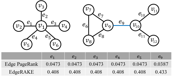
Figure 1: An example network $\mathcal{G}$

Furthermore, despite considerable research Kucharczuk et al. (2022); Murai and Yoshida (2019); Bao et al. (2022) invested in theoretical analysis of these edge centrality metrics, to our knowledge, none of the extant studies have explored their practical effectiveness in downstream graph analytics tasks. Therefore, it still remains unclear which edge centrality metrics should be adopted in real applications.

In this paper, we first propose a new centrality measure EdgeRAKE (Edge Ranking via rAndom walK with rEstart) for edge ranking in directed/undirected and weighted/unweighted networks. EdgeRAKE tweaks the random walk with restart model Tong et al. (2006) for nodes to adapt edges with consideration of the topological connections pertinent to both endpoints of an edge as well as the importance of their respective influences. If we revisit the example in Fig. 1, the issue of edge PageRank is now resolved when EdgeRAKE is utilized ($0.433>0.408$). We further present an approximate algorithm for EdgeRAKE computation that runs in time linear to the size of $\mathcal{G}$. A thorough theoretical analysis in terms of its properties, convergence, approximation accuracy guarantees, and time complexity is then conducted. We demonstrate the superiority of EdgeRAKE over existing edge centrality measures in empirical effectiveness through extensive experiments on six real datasets in three popular network tasks involving graph clustering, network embedding, and graph neural networks.

2 Preliminaries

2.1 Notations and Terminology

Throughout this paper, sets are symbolized by calligraphic letters, e.g., $\mathcal{V}$, and $|\mathcal{V}|$ is used to denote the cardinality of the set $\mathcal{V}$. Matrices (resp. vectors) are represented as bold uppercase (resp. lowercase) letters, e.g., $\mathbf{A}$ (resp. $\mathbf{x}$). We use superscript $\mathbf{A}^{\top}$ to represent the transpose of matrix $\mathbf{A}$. $\mathbf{A}[i,j]$ denotes the $(i,j)$-th entry in matrix $\mathbf{A}$.

Let $\mathcal{G}=(\mathcal{V},\mathcal{E})$ be a network (a.k.a. graph) with a node set $\mathcal{V}$ containing $n$ nodes and an edge set $\mathcal{E}$ consisting of $m$ edges. Each edge $e=(u,v)\in\mathcal{E}$ is associated with a positive weight $w(e)$ or $w(u,v)$, which is equal to 1 when $\mathcal{G}$ is unweighted. For each node $v\in\mathcal{V}$, we denote by $\mathcal{N}^{-}(v)$ (resp. $\mathcal{N}^{+}(v)$) the set of incoming (resp. outgoing) neighbors of $v$. Particularly, $\mathcal{N}^{-}(v)=\mathcal{N}^{+}(v)$ when $\mathcal{G}$ is undirected. We use the diagonal matrix $\mathbf{D}$ to represent the out-degree matrix of $\mathcal{G}$, where each diagonal element $\mathbf{D}[v,v]=\sum_{u\in\mathcal{N}^{+}(v)}{w(v,u)}$, which is $|\mathcal{N}^{+}(v)|$ when $\mathcal{G}$ is unweighted. The adjacency matrix of $\mathcal{G}$ is symbolized by $\mathbf{A}$, in which $\mathbf{A}[u,v]=w(u,v)$ if $(u,v)\in\mathcal{E}$, otherwise $0$. The incidence matrix of $\mathcal{G}$ is denoted by $\mathbf{E}\in\mathbb{R}^{n\times m}$, wherein $\mathbf{E}[v_{i},e_{i}]=w(e_{i})$ if node $v_{i}$ is incident with edge $e_{i}$, and $\mathbf{E}[v_{i},e_{i}]=0$ otherwise. Based thereon, we define the column-normalized incidence matrix of $\mathcal{G}$ as $\widehat{\mathbf{E}}\in\mathbb{R}^{n\times m}$, whose $(v_{i},e_{i})$-entry $\widehat{\mathbf{E}}[v_{i},e_{i}]$ is $\frac{\mathbf{E}[v_{i},e_{i}]}{\sum_{v\in V}{\mathbf{E}[v,e_{i}]}}$.

2.2 Existing Edge Centrality Measures

Table 1: Existing Edge Centralities

Centrality	Edge Direction	Edge Weight	Definition	Complexity
Edge Betweenness (EB) Girvan and Newman (2002)	✓	✗	Eq. (1)	$O(n^{2}+mn)$
$\kappa$-Path Edge Centrality (KPC) De Meo et al. (2012)	✓	✗	-	$O(m+n^{2}\kappa)$
Effective Resistance (ER) Spielman and Srivastava (2008)	✗	✗	Eq. (2)	$O(mn^{\frac{3}{2}})$
BDRC Yi et al. (2018)	✗	✓	Eq. (3)	$O(m+n^{3})$
Edge PageRank (EP) Chapela et al. (2015)	✓	✓	Eq. (4)	$O(m)$
Edge Katz (EK) Chapela et al. (2015)	✓	✓	Eq. (5)	$O(m)$
Eigenedge (EE) Huang and Huang (2019)	✓	✓	-	$O(m)$
Information Centrality (IC) Fortunato et al. (2004)	✓	✗	-	$O(mn^{2}\log{n})$
$\theta$-Kirchhoff Edge Centrality ($\theta$-KEC) Li and Zhang (2018)	✗	✓	-	$O(mn^{3})$
Kemeny Edge Centrality (KEC) Altafini et al. (2023)	✗	✗	-	$O(m^{2}n)$
GTOM Yip and Horvath (2007)	✓	✗	Eq. (6)	$O(m\cdot\max_{v\in V}{|\mathcal{N}^{+}(v)|})$
Current-Flow Centrality (CFC) Brandes and Fleischer (2005)	✓	✗	-	$O(mn\log{n})$
Our EdgeRAKE (ERK)	✓	✓	Eq. (9)	$O(m)$

In what follows, we categorize existing edge centrality metrics in the literature into four groups and review each of them.

Ratio-based Edge Centralities. At a high level, this category of centralities utilizes the fraction of paths or spanning trees containing target edge $e=(u,v)$ to quantify the importance of $e$ in the network $\mathcal{G}$. Amid them, edge betweenness (EB) Girvan and Newman (2002) is one of the most classic measures, which is formally defined by

$$C_{\text{EB}}(e)=\sum_{s\neq t\in V}{\frac{\delta_{s,t}(e)}{\delta_{s,t}}},$$ (1)

where $\delta_{s,t}$ signifies the number of shortest paths from $s$ to $t$ and $\delta_{s,t}(e)$ is the number of such paths passing through edge $e$. However, EB falls short of considering arbitrary paths that embody rich topological information Stephenson and Zelen (1989). As a remedy, in De Meo et al. (2012), the authors extend the $\kappa$-path centrality Alahakoon et al. (2011) for nodes to edges, dubbed as $\kappa$-path edge centrality (KPC). More precisely, KPC $C_{\text{KPC}}(e)$ is the sum of the factions $\frac{\delta_{s}(e)}{\delta_{s}}$ of length-$\kappa$ paths originating from every node $s\in V$ traversing edge $e$.

In lieu of using paths as in EB and KPC, effective resistance (ER) Lovász (1993) (a.k.a. spanning edge betweenness/centrality Teixeira et al. (2013) or resistance distance) relies on minimum spanning trees (MSTs). Formally, the ER of edge $e=(u,v)$ is formulated as

$$C_{\text{ER}}(e)=\frac{\tau_{G}(e)}{\tau_{G}},$$ (2)

where $\tau_{G}$ is the number of distinct MSTs from $\mathcal{G}$ and $\tau_{G}(e)$ represents the number of distinct MSTs from $\mathcal{G}$ where edge $e$ occurs. According to Spielman and Srivastava (2008), Eq. (2) can be equivalently rewritten as:

$$C_{\text{ER}}(e)=\mathbf{L}^{\dagger}[u,u]+\mathbf{L}^{\dagger}[v,v]-2\mathbf{L}^{\dagger}[u,v],$$

where $\mathbf{L}^{\dagger}$ denotes the Moore-Penrose pseudo-inverse of the Laplacian (i.e., $\mathbf{L}=\mathbf{D}-\mathbf{A}$) of $\mathcal{G}$. Yi et al. (2018) pinpoints that ER fails to distinguish any pair of cut edges, and then based on Lipman et al. (2010) proposes a variant of ER, i.e., biharmonic distance related centrality (BDRC) in Eq. (3) as a remedy.

$$C_{\text{BDRC}}(e)=w(u,v)^{2}\cdot\left({\mathbf{L}^{\dagger}}^{2}[u,u]+{\mathbf{L}^{\dagger}}^{2}[v,v]-2{\mathbf{L}^{\dagger}}^{2}[u,v]\right)$$ (3)

Recursive-based Edge Centralities. Another line of research resorts to a recursive definition. That is, the influence of an edge $e=(u,v)$ is proportional to the sum of the influence scores of other edges incoming to its starting point $u$. In the spirit of such an idea, Chapela et al. (2015) extends prominent node-wise centrality measure PageRank Page et al. (1998) to edge PageRank (EP) in Eq. (4), where the EP of edge $e=(u,v)$ is contributed by the EP values of all edges incident to the start node $u$ and its self-importance. The parameter $\alpha\in(0,1)$ is used to control the importance of the influence from such incoming edges.

$$C_{\text{EP}}(e)=\frac{w(u,v)}{\mathbf{D}[u,u]}\left(\alpha\ \sum_{x\in\mathcal{N}^{-}(u)}{C_{\text{EP}}((x,u))}+1\right)$$ (4)

Akin to EP, Chapela et al. (2015) further extends Katz index Katz (1953) to Edge Katz (EK) as follows:

$$C_{\text{EK}}(e)=w(u,v)\cdot\left(\alpha\sum_{x\in\mathcal{N}^{-}(u)}{C_{\text{EK}}((x,u))}+1\right),$$ (5)

Huang and Huang (2019) extends eigencentrality for nodes Bonacich (1972) to Eigenedge (EE), which can be regarded as a variant of EK.

Leave-One-Out Edge Centralities. In this category, the importance of an edge $e=(u,v)$ is evaluated by the change after excluding $e$ from $\mathcal{G}$ in terms of a network metric. For example, the information centrality (IC) Fortunato et al. (2004) of $e$ is defined as the relative loss in the network efficiency obtained by removing $e=(u,v)$ from $\mathcal{G}$: $C_{\text{IC}}(e)=\frac{\epsilon(G)-\epsilon(G\setminus e)}{\epsilon(G)},$ where $\epsilon(G)$ connotes the average network efficiency (i.e., the reciprocal of the distance of two nodes) Latora and Marchiori (2001) of $\mathcal{G}$ and can be calculated by $\epsilon(G)=\frac{1}{n(n-1)}\sum_{u\neq v\in V}{\frac{1}{distance(u,v)}}.$ In analogy to IC, $\theta$-Kirchhoff edge centrality ($\theta$-KEC) of edge $e$ is defined as the Kirchhoff index of the network obtained from $\mathcal{G}$ by deleting $e$ Li and Zhang (2018), where the Kirchhoff index of a network is the sum of effective resistances of all node pairs. Very recently, Altafini et al. (2023) propose Kemeny-based Edge Centrality (KEC): $C_{\text{KEC}}(e)=K(G\setminus{e})-K(G),$ where $K(G)$ represents the Kemeny’s constant Kemeny and Snell (1960) of $\mathcal{G}$, i.e., the expected number of time steps needed from a starting node $u$ to a random destination node $v$ sampled from the stationary distribution of the Markov chain induced by the transition matrix of $\mathcal{G}$.

Others. As in Eq. (6), the generalized topological overlap matrix (GTOM) Yip and Horvath (2007) of $e$ simply measures the amount of common direct successors that the start and end nodes of $e$ share.

$$C_{\text{GTOM}}(e)=\frac{|\mathcal{N}^{+}(u)\cap\mathcal{N}^{+}(v)|+1}{\min\{|\mathcal{N}^{+}(u)|,|\mathcal{N}^{+}(v)|\}}$$ (6)

The current-flow centrality (CFC) Brandes and Fleischer (2005) leverages the number of flows between any two nodes $s,t\in V$ that pass through $e$ as its centrality.

Table 1 summarizes the properties and computational complexities of the above 12 edge centrality metrics. Note that only three existing edge centrality measures, i.e., EP, EK, and EE, can be applied to directed and weighted edges and achieve a linear asymptotic performance. By Chapela et al. (2015), $C_{\text{EP}}(e)$ and $C_{\text{EK}}(e)$ are reweighted versions of PageRank $PR(u)$ and Katz index $KA(u)$ of node $u$, respectively, i.e., $C_{\text{EP}}(e)=\frac{w(u,v)}{\mathbf{D}[u,u]}\cdot PR(u),\ C_{\text{EK}}(e)=w(u,v)\cdot KA(u).$ Such a definition overlooks the topological influences from other edges on $e$ via node $v$, leading to undermined edge ranking quality. EE has the same flaw as it is a special case of EK. In addition, EK produces extremely high centrality values, rendering it hard to distinguish vital edges from trivial ones. EP assumes $G$ to be connected, and hence, fails on disconnected networks, as exemplified in Fig. 1.

3 EdgeRAKE

In this section, we first elaborate on the design of EdgeRAKE, followed by the algorithmic details for computing EdgeRAKE and related theoretical analysis.

3.1 Edge-wise Random Walk with Restart

Given a weighted network $\mathcal{G}$, a jumping probability $\alpha$, a source edge $e_{s}=(u_{s},v_{s})$ and a target edge $e_{t}=(u_{t},v_{t})$, an edge-wise random walk with restart (ERWR) on $\mathcal{G}$ starts from $e_{s}$. Next, at each step, the walk either (i) terminates at the current edge $e_{i}=(u_{i},v_{i})$ with a probability of $1-\alpha$; or (ii) with the remaining $\alpha$ probability, jumps to node $u_{j}$ that is incident with $e_{i}$ ($u_{j}=v_{i}$ when $\mathcal{G}$ is directed and $u_{j}=u_{i}$ or $v_{i}$ with an equal likelihood when $\mathcal{G}$ is undirected), and subsequently navigates to one of the out-going edges $(u_{j},v_{j})$ of the current node $u_{j}$ (i.e., $u_{i}$ or $v_{i}$) according to the following probability:

$$\frac{w(u_{j},v_{j})}{\sum_{(u_{j},v_{x})\in\mathcal{E}}{w(u_{j},v_{x})}}.$$ (7)

We refer to the probability of the above walk from $e_{s}$ stopping at $e_{t}$ in the end as the ERWR score of $e_{t}$ w.r.t. $e_{s}$ and denote it by $r(e_{s},e_{t})$. Lemma 1 presents the mathematical definition of $r(e_{s},e_{t})$.

Lemma 1.

The ERWR score $r(e_{s},e_{t})$ of $e_{t}$ w.r.t. $e_{s}$ can be computed via

$$r(e_{s},e_{t})=\sum_{\ell=0}^{\infty}{(1-\alpha)\alpha^{\ell}\cdot{\left(\widehat{\mathbf{E}}^{\top}\mathbf{D}^{-1}\mathbf{E}\right)}^{\ell}}[e_{s},e_{t}].$$ (8)

Proof.

As per the definitions of $\mathbf{E}$ and $\mathbf{D}$, we can rewrite Eq. (7) to its equivalent form $(\mathbf{D}^{-1}\mathbf{E})[u_{j},e_{j}]$. Hence, the probability of jumping from $e_{i}=(u_{i},v_{i})$ to $e_{j}=(u_{j},v_{j})$ via $u_{j}=u_{i}$ or $u_{j}=v_{i}$ with one step in an ERWR is as follows:

$$\sum_{u_{j}\in e_{i}}{\frac{\mathbf{E}^{\top}[e_{i},u_{j}]}{\sum_{v\in V}{\mathbf{E}^{\top}[e_{i},v]}}\cdot(\mathbf{D}^{-1}\mathbf{E})[u_{j},e_{j}]}=\left(\widehat{\mathbf{E}}^{\top}\mathbf{D}^{-1}\mathbf{E}\right)[e_{i},e_{j}].$$

As such, the probability of an ERWR originating from $e_{s}$ visiting $e_{t}$ at $\ell$-th step is

$$\alpha^{\ell}\left(\widehat{\mathbf{E}}^{\top}\mathbf{D}^{-1}\mathbf{E}\right)^{\ell}[e_{s},e_{t}].$$

Recall that at each step, the walk terminates at its current node with a probability of $1-\alpha$. Then, the probability of an ERWR originating from $e_{s}$ ending at $e_{t}$ at $\ell$-th step is $(1-\alpha)\alpha^{\ell}\left(\widehat{\mathbf{E}}^{\top}\mathbf{D}^{-1}\mathbf{E}\right)^{\ell}[e_{s},e_{t}]$. By considering all steps that the walk might stop at, we can obtain the overall ERWR value in Eq. (8), completing the proof. ∎

Intuitively, $r(e_{s},e_{t})$ quantifies the strength of multi-hop connections from $e_{s}$ to $e_{t}$ with consideration of the edge directions and weights, which can be interpreted as the total direct and indirect influences of $e_{s}$ on $e_{t}$.

Definition of EdgeRAKE. Akin to the recursive-based edge centrality measures introduced in Section 2.2, we define the EdgeRAKE $C_{\text{ERK}}(e)$ of edge $e=(u,v)$ as the weighted sum of ERWR scores of $e$ w.r.t. the all possible source edges $e_{i}$ in $\mathcal{G}$:

$$C_{\text{ERK}}(e)=\sum_{e_{i}=(u_{i},v_{i})\in\mathcal{E}}{\frac{w(e_{i})\cdot r(e_{i},e)}{\sqrt{\mathbf{D}[u_{i},u_{i}]+\mathbf{D}[v_{i},v_{i}]}}},$$ (9)

where each source edge $e_{i}$ is weighted by $\frac{w(e_{i})}{\sqrt{\mathbf{D}[u_{i},u_{i}]+\mathbf{D}[v_{i},v_{i}]}}$. This weight is to reflect the importance of $e_{i}$’s influence (ERWR score) on $e$ from the perspective of the whole $\mathcal{G}$. The intuition is that an edge $e_{i}$ is less important to $\mathcal{G}$ if its edge weight $w(e_{i})$ is small or its endpoints are connected to a multitude of edges with high edge weights (i.e., $\mathbf{D}[u_{i},u_{i}]+\mathbf{D}[v_{i},v_{i}]$ is large). As such, deleting it from $\mathcal{G}$ will engender an insignificant impact on other edges. Consequently, we assign a low weight $\frac{w(e_{i})}{\sqrt{\mathbf{D}[u_{i},u_{i}]+\mathbf{D}[v_{i},v_{i}]}}$ to its influence, i.e., ERWR $r(e_{i},e)$. In particular, when $\mathcal{G}$ is unweighted, this weight is equal to $\frac{1}{\sqrt{|\mathcal{N}^{+}(u_{i})|+|\mathcal{N}^{+}(v_{i})|}}$.

Algorithm 1 EdgeRAKE Computation

Input: Network $G=(V,E)$
Parameter: Jumping probability $\alpha$, the number $t$ of iterations
Output: $C^{\prime}_{\text{ERK}}(e)\ \forall{e\in\mathcal{E}}$

1:  Initialize a row vector $\mathbf{x}\in\mathbb{R}^{m}$.

2:  for $e_{i}=(u_{i},v_{i})\in\mathcal{E}$ do

3:     $\mathbf{x}[e_{i}]\leftarrow\frac{w(e_{i})}{\sqrt{\mathbf{D}[u_{i},u_{i}]+\mathbf{D}[v_{i},v_{i}]}}$.

4:  end for

5:  $\mathbf{z}\leftarrow\mathbf{x}$

6:  for $i\leftarrow 1$ to $t$ do

7:     $\mathbf{z}\leftarrow{\alpha}\cdot\mathbf{z}\widehat{\mathbf{E}}^{\top}\mathbf{D}^{-1}\mathbf{E}+\mathbf{x}$.

8:  end for

9:  for $e\in\mathcal{E}$ do

10:     $C^{\prime}_{\text{ERK}}(e)\leftarrow(1-\alpha)\cdot\mathbf{z}[e]$.

11:  end for

12:  return $C^{\prime}_{\text{ERK}}(e)\ \forall{e\in\mathcal{E}}$

3.2 Algorithm

In Algo. 1, we display the pseudo-code for approximating EdgeRAKE of all edges in $\mathcal{G}$. Algo. 1 begins by taking as input the network $\mathcal{G}$, jumping probability $\alpha$, and the number $t$ of iterations. Afterwards, Algo. 1 initializes a length-$m$ row vector $\mathbf{x}$, in which each entry corresponds to an edge’s initial importance, i.e., $\mathbf{x}[e_{i}]=\frac{w(e_{i})}{\sqrt{\mathbf{D}[u_{i},u_{i}]+\mathbf{D}[v_{i},v_{i}]}}$ for edge $e_{i}=(u_{i},v_{i})$ (Lines 1-4). After setting $\mathbf{z}=\mathbf{x}$ at Line 5, Algo. 1 starts an iterative process to update $\mathbf{z}$ (Lines 6-8). Specifically, in each iteration, we compute a new $\mathbf{z}$ by

$$\mathbf{z}={\alpha}\cdot\left(\mathbf{z}\widehat{\mathbf{E}}^{\top}\right)\cdot\mathbf{D}^{-1}\mathbf{E}+\mathbf{x}.$$ (10)

We repeat the above step for $t$ iterations and then compute $C^{\prime}_{\text{ERK}}(e)$ for each edge $e\in\mathcal{E}$ by $C^{\prime}_{\text{ERK}}(e)=(1-\alpha)\cdot\mathbf{z}[e].$ Finally, Algo. 1 returns $C^{\prime}_{\text{ERK}}(e)\ \forall{e\in\mathcal{E}}$ as the approximate EdgeRAKE values of all edges in $\mathcal{G}$.

3.3 Analysis

First, Lemma 2 indicates two crucial properties of ${\left(\widehat{\mathbf{E}}^{\top}\mathbf{D}^{-1}\mathbf{E}\right)}^{\ell}$, a key constituent part of EdgeRAKE values.

Lemma 2.

Given $\mathcal{G}$ and any integer $\ell\geq 1$, the matrix ${\left(\widehat{\mathbf{E}}^{\top}\mathbf{D}^{-1}\mathbf{E}\right)}^{\ell}$ satisfies the following two properties:

• Property 1: ${\left(\widehat{\mathbf{E}}^{\top}\mathbf{D}^{-1}\mathbf{E}\right)}^{\ell}$ is a non-negative row-stochastic matrix, and a non-negative doubly stochastic matrix when $\mathcal{G}$ is unweighted;

• Property 2: $\forall{e_{i},e_{j}\in G}$, $w(e_{i})\cdot{\left(\widehat{\mathbf{E}}^{\top}\mathbf{D}^{-1}\mathbf{E}\right)}^{\ell}[e_{i},e_{j}]=w(e_{j})\cdot{\left(\widehat{\mathbf{E}}^{\top}\mathbf{D}^{-1}\mathbf{E}\right)}^{\ell}[e_{j},e_{i}].$

Proof.

First, we prove that $\widehat{\mathbf{E}}^{\top}\mathbf{D}^{-1}\mathbf{E}$ is a non-negative row-stochastic matrix. Consider any edge $e_{i}$ in $\mathcal{E}$. We have

$$\sum_{e_{j}\in\mathcal{E}}{\left(\widehat{\mathbf{E}}^{\top}\mathbf{D}^{-1}\mathbf{E}\right)[e_{i},e_{j}]}=\sum_{e_{j}\in\mathcal{E}}\sum_{v\in V} \widehat{\mathbf{E}}^{\top}[e_{i},v]\cdot(\mathbf{D}^{-1}\mathbf{E})[v,e_{j}]$$

$$=\sum_{v\in V}\widehat{\mathbf{E}}^{\top}[e_{i},v]\sum_{e_{j}\in\mathcal{E}}(\mathbf{D}^{-1}\mathbf{E})[v,e_{j}] =\sum_{v\in V}\widehat{\mathbf{E}}^{\top}[e_{i},v]=1,$$

which implies that ${\left(\widehat{\mathbf{E}}^{\top}\mathbf{D}^{-1}\mathbf{E}\right)}^{\ell}$ is also a non-negative row-stochastic matrix. Particularly, when $\mathcal{G}$ is unweighted, i.e., $w(e)=1\ \forall{e\in\mathcal{E}}$, $\widehat{\mathbf{E}}^{\top}$ is equal to $\mathbf{E}^{\top}$ and $\frac{1}{2}\mathbf{E}^{\top}$ if $\mathcal{G}$ is directed and undirected, respectively. Accordingly, $\widehat{\mathbf{E}}^{\top}\mathbf{D}^{-1}\mathbf{E}$ is a symmetric matrix, indicating that $\widehat{\mathbf{E}}^{\top}\mathbf{D}^{-1}\mathbf{E}$ and ${\left(\widehat{\mathbf{E}}^{\top}\mathbf{D}^{-1}\mathbf{E}\right)}^{\ell}$ are non-negative doubly stochastic, i.e., $\sum_{e_{i}\in\mathcal{E}}{\left(\widehat{\mathbf{E}}^{\top}\mathbf{D}^{-1}\mathbf{E}\right)}^{\ell}[e_{i},e]=1.$

Next, we prove Property 2. Notice that $\widehat{\mathbf{E}}^{\top}$ can be represented by $\mathbf{D}_{E}^{-1}\mathbf{E}^{\top}$ where $\mathbf{D}_{E}$ is a diagonal matrix and each entry $\mathbf{D}_{E}[e_{i},e_{i}]=\sum_{v\in V}{\mathbf{E}[v,e_{i}]}$, which equals to $w(e_{i})$ and $2w(e_{i})$ when $\mathcal{G}$ is directed and undirected, respectively. For any integer $\ell\geq 1$, ${\left(\widehat{\mathbf{E}}^{\top}\mathbf{D}^{-1}\mathbf{E}\right)}^{\ell}\mathbf{D}_{E}^{-1}={\left(\mathbf{D}_{E}^{-1}\mathbf{E}^{\top}\mathbf{D}^{-1}\mathbf{E}\right)}^{\ell}\mathbf{D}_{E}^{-1}$ is a symmetric matrix, meaning that ${\left(\widehat{\mathbf{E}}^{\top}\mathbf{D}^{-1}\mathbf{E}\right)}^{\ell}[e_{i},e_{j}]\cdot\mathbf{D}^{-1}_{E}[e_{j},e_{j}]={\left(\widehat{\mathbf{E}}^{\top}\mathbf{D}^{-1}\mathbf{E}\right)}^{\ell}[e_{j},e_{i}]\cdot\mathbf{D}^{-1}_{E}[e_{i},e_{i}]$. Therefore, the second property is proven. ∎

Based on these two properties, we can derive the following bounds for EdgeRAKE $C_{\text{ERK}}(e)$ defined in Eq. (9).

Lemma 3.

Given $\mathcal{G}$, the EdgeRAKE $C_{\textnormal{ERK}}(e)$ is in the range $[\frac{w(e)}{\underset{{e_{i}\in\mathcal{E}}}{\max}{\sqrt{\mathbf{D}[u_{i},u_{i}]+\mathbf{D}[v_{i},v_{i}]}}},\frac{w(e)}{\underset{{e_{i}\in\mathcal{E}}}{\min}{\sqrt{\mathbf{D}[u_{i},u_{i}]+\mathbf{D}[v_{i},v_{i}]}}}]$.

Proof.

By Property 2 in Lemma 2, for any two edges $e_{i},e_{j}\in\mathcal{E}$, $w(e_{i})\cdot r(e_{i},e_{j})=w(e_{j})\cdot r(e_{j},e_{i})$. Hence, $C_{\text{ERK}}(e)=\sum_{e_{i}=(u_{i},v_{i})\in\mathcal{E}}{\frac{w(e_{i})\cdot r(e_{i},e)}{\sqrt{\mathbf{D}[u_{i},u_{i}]+\mathbf{D}[v_{i},v_{i}]}}}=\sum_{e_{i}=(u_{i},v_{i})\in\mathcal{E}}{\frac{w(e)\cdot r(e,e_{i})}{\sqrt{\mathbf{D}[u_{i},u_{i}]+\mathbf{D}[v_{i},v_{i}]}}},$ leading to $C_{\text{ERK}}(e)\leq\underset{{e\in\mathcal{E}}}{\min}{\sqrt{\mathbf{D}[u_{i},u_{i}]+\mathbf{D}[v_{i},v_{i}]}}\cdot\sum_{e_{i}\in\mathcal{E}}{r(e,e_{i})}$ and $C_{\text{ERK}}(e)\geq\underset{{e\in\mathcal{E}}}{\max}{\sqrt{\mathbf{D}[u_{i},u_{i}]+\mathbf{D}[v_{i},v_{i}]}}\cdot\sum_{e_{i}\in\mathcal{E}}{r(e,e_{i})}$. Next, by Eq. (8) and Property 1 in Lemma 2, we can get $\sum_{e_{i}\in\mathcal{E}}{r(e,e_{i})}=1$, which seals the proof. ∎

Convergence Analysis. Mathematically, we can express the convergence of EdgeRAKE as: $\lim_{t\to\infty}{\|\mathbf{z}^{(t)}-\mathbf{z}^{(t-1)}\|_{2}}=0$. Note that Algo. 1 is essentially a power method Mises and Pollaczek-Geiringer (1929). As per the Perron-Frobenius theorem Pillai et al. (2005) and the stochastic property of $\widehat{\mathbf{E}}^{\top}\mathbf{D}^{-1}\mathbf{E}$ in Lemma 2, if $\mathcal{G}$ is connected and unipartite, and each node has out-going edges, $(1-\alpha)\mathbf{z}$ in Algo. 1 converges to the scaled dominant eigenvector of the matrix $\widehat{\mathbf{E}}^{\top}\mathbf{D}^{-1}\mathbf{E}$ and the convergence rate is the second largest eigenvalue of $\widehat{\mathbf{E}}^{\top}\mathbf{D}^{-1}\mathbf{E}$ Langville and Meyer (2006). If $\mathcal{G}$ is not connected and can be divided into components $\mathcal{G}_{1},\mathcal{G}_{2},\cdots,\mathcal{G}_{k}$ that are unipartite, for edges in each component $\mathcal{G}_{i}$, their corresponding entries in $(1-\alpha)\mathbf{z}$ will converge to the scaled dominant eigenvector of $\mathcal{G}_{i}$’s corresponding matrix block in $\widehat{\mathbf{E}}^{\top}\mathbf{D}^{-1}\mathbf{E}$.

Approximation Analysis. On the basis of Lemma 2, we can establish the approximation accuracy guarantees for Algo. 1.

Theorem 4.

Let $C^{\prime}_{\textnormal{ERK}}(e)\ \forall{e\in\mathcal{E}}$ be the output of Algo. 1 and $t=\log_{\alpha}{\epsilon}-1$. Then, for each edge $e\in\mathcal{E}$, the following inequality holds:

$$0\leq C_{\textnormal{ERK}}(e)-C^{\prime}_{\textnormal{ERK}}(e)\leq\frac{w(e)\cdot\epsilon}{\underset{{(u_{i},v_{i})\in\mathcal{E}}}{\min}{\sqrt{\mathbf{D}[u_{i},u_{i}]+\mathbf{D}[v_{i},v_{i}]}}}.$$ (11)

In particular, when $\mathcal{G}$ is unweighted,

$$0\leq C_{\textnormal{ERK}}(e)-C^{\prime}_{\textnormal{ERK}}(e)\leq\frac{\epsilon}{\sqrt{2}}.$$ (12)

Proof.

First, we denote a truncated version of $r(e_{i},e)$ by $r^{\prime}(e_{i},e)=\sum_{\ell=0}^{t}{(1-\alpha)\alpha^{\ell}\cdot{\left(\widehat{\mathbf{E}}^{\top}\mathbf{D}^{-1}\mathbf{E}\right)}^{\ell}}[e_{i},e]$. By induction, it can be shown that $\mathbf{z}$ obtained after $t$ iterations of Line 7 can be represented by $\mathbf{z}=\mathbf{x}\sum_{\ell=0}^{t}{\alpha^{\ell}\cdot{\left(\widehat{\mathbf{E}}^{\top}\mathbf{D}^{-1}\mathbf{E}\right)}^{\ell}}.$ Hence, we have $\mathbf{z}[e]=\frac{1}{1-\alpha}\sum_{e_{i}\in\mathcal{E}}{\mathbf{x}[e_{i}]\cdot r^{\prime}(e_{i},e)}$ and $C^{\prime}_{\textnormal{ERK}}(e)=\sum_{e_{i}\in\mathcal{E}}{\mathbf{x}[e_{i}]\cdot r^{\prime}(e_{i},e)}=\sum_{e_{i}=(u_{i},v_{i})\in\mathcal{E}}{\frac{w(e_{i})\cdot r^{\prime}(e_{i},e)}{\sqrt{\mathbf{D}[u_{i},u_{i}]+\mathbf{D}[v_{i},v_{i}]}}}.$ By the definition of exact EdgeRAKE in Eq. (9), we obtain

$$C_{\textnormal{ERK}}(e)-C^{\prime}_{\textnormal{ERK}}(e)=\sum_{e_{i}=(u_{i},v_{i})\in\mathcal{E}}{\frac{w(e_{i})\cdot(r(e_{i},e)-r^{\prime}(e_{i},e))}{\sqrt{\mathbf{D}[u_{i},u_{i}]+\mathbf{D}[v_{i},v_{i}]}}}$$

$$=\sum_{e_{i}=(u_{i},v_{i})\in\mathcal{E}}{\frac{w(e_{i})\cdot\sum_{\ell=t+1}^{\infty}{(1-\alpha)\alpha^{\ell}\cdot{\left(\widehat{\mathbf{E}}^{\top}\mathbf{D}^{-1}\mathbf{E}\right)}^{\ell}}[e_{i},e]}{\sqrt{\mathbf{D}[u_{i},u_{i}]+\mathbf{D}[v_{i},v_{i}]}}}.$$ (13)

By leveraging Properties 1 and 2 in Lemma 2 and the fact $\sum_{\ell=t+1}^{\infty}{(1-\alpha)\alpha^{\ell}}=1-\sum_{\ell=0}^{t}{(1-\alpha)\alpha^{\ell}}=\alpha^{t+1}=\epsilon$, we can further transform Eq. (13) as follows:

$$\sum_{e_{i}=(u_{i},v_{i})\in\mathcal{E}}{\frac{w(e_{i})\sum_{\ell=t+1}^{\infty}{(1-\alpha)\alpha^{\ell}{\left(\widehat{\mathbf{E}}^{\top}\mathbf{D}^{-1}\mathbf{E}\right)}^{\ell}}[e,e_{i}]\cdot\frac{w(e)}{w(e_{i})}}{\sqrt{\mathbf{D}[u_{i},u_{i}]+\mathbf{D}[v_{i},v_{i}]}}}$$

$$\leq\frac{w(e)\cdot\sum_{\ell=t+1}^{\infty}{(1-\alpha)\alpha^{\ell}\sum_{e_{i}\in\mathcal{E}}{\left(\widehat{\mathbf{E}}^{\top}\mathbf{D}^{-1}\mathbf{E}\right)}^{\ell}}[e,e_{i}]}{\underset{{(u_{i},v_{i})\in\mathcal{E}}}{\min}{\sqrt{\mathbf{D}[u_{i},u_{i}]+\mathbf{D}[v_{i},v_{i}]}}}$$

$$=\frac{w(e)\cdot\sum_{\ell=t+1}^{\infty}{(1-\alpha)\alpha^{\ell}}}{\underset{{(u_{i},v_{i})\in\mathcal{E}}}{\min}{\sqrt{\mathbf{D}[u_{i},u_{i}]+\mathbf{D}[v_{i},v_{i}]}}}=\frac{w(e)\cdot\epsilon}{\underset{{(u_{i},v_{i})\in\mathcal{E}}}{\min}{\sqrt{\mathbf{D}[u_{i},u_{i}]+\mathbf{D}[v_{i},v_{i}]}}},$$

proving the correctness of Eq. (11). When $\mathcal{G}$ is unweighted, i.e., $w(e)=1\ \forall{e\in\mathcal{E}}$, Eq. (12) naturally follows. ∎

Complexity Analysis. According to Algo. 1, the computation expenditure for approximate EdgeRAKE values of all edges in the input network $\mathcal{G}$ lies in the $t$ iterations of matrix multiplications (Lines 6-7). Note that $\widehat{\mathbf{E}}$ and $\mathbf{E}$ are sparse matrices containing $m$ non-zero entries, and we can utilize the trick in Eq. (10) to reorder the sparse matrix-vector multiplications for higher efficiency. In doing so, the execution of Line 6 takes $O(m)$ time, and thus, the time complexity for $t$ iterations is $O(mt)$ in total. Since the number $t$ of iterations can be regarded as a constant, Algo. 1 runs in $O(m)$ time.

4 Experiments

In this section, we empirically study the effectiveness of EdgeRAKE and existing edge centralities for identifying influential edges in six real-world networks through three popular graph analytics tasks, i.e., graph clustering, unsupervised network embedding, and graph neural networks, as well as their computation efficiency.

4.1 Experimental Setup

Table 2: Statistics of Datasets

Name	#Nodes	#Edges	#Attributes	#Classes
Email-EU	1,005	25,571	-	-
Facebook	4,039	88,234	-	-
PPI	3,890	76,584	-	50
BlogCatalog	10,312	333,983	-	39
Cora	2,708	10,556	1,433	7
Chameleon	2,277	62,792	2,325	5

Environment. All the experiments were conducted on a Linux machine powered by 2 Xeon Gold 6330 @2.0GHz CPUs and 1TB RAM. All the proposed methods were implemented in Python. For Edge Betweenness, we employ the NetworkX package Hagberg et al. (2008) for computation.

Datasets. We experiment with six real networks whose statistics are listed in Table 2. Email-EU Leskovec et al. (2007) includes emails between members of a large research institution in Europe, whereas the Facebook dataset Leskovec and Mcauley (2012) contains participated Facebook users and their friendships, both of which are collected from SNAP Leskovec and Krevl (2014). As for the PPI and BlogCatalog, they are two popular datasets used in network embedding (NE) Grover and Leskovec (2016). The PPI dataset is a subgraph of the protein-to-protein interaction network for Homo Sapiens, wherein node labels are obtained from the hallmark gene sets and represent biological states. BlogCatalog is a network of social relationships among the bloggers on the BlogCatalog website, where node labels correspond to the interests of bloggers. Moreover, we include two well-known benchmark datasets for graph neural networks (GNNs), i.e., Cora Yang et al. (2016) and Chameleon Rozemberczki et al. (2021). We download and preprocess them using the PyTorch Geometric Library Fey and Lenssen (2019).

Competing Edge Centralities. We evaluate our proposed EdgeRAKE against six best competitors, EB, ER, EP, EK, GTOM, and BDRC, out of all the edge centrality measures listed in Table 1. We exclude KPC, KEC, CFC, and IC from comparison due to their extremely high computation overheads. Additionally, EE can be regarded as a variant of EP or EK, and thus, is omitted. Unless specified otherwise, for EP, EK, and EdgeRAKE, we set $\alpha=0.5$ and the maximum number of iterations to $150$. For reproducibility, all the codes and datasets are made publicly available at https://github.com/HKBU-LAGAS/EdgeRAKE.

4.2 Effectiveness Evaluation

In this set of experiments, we evaluate the effectiveness of EdgeRAKE and competing edge centralities as follows. After calculating the centrality values of the edges, we sort all edges of the input network $G$ in ascending order by their centrality values. Then, we remove the top-$(m\cdot\rho)$ ($\rho$ is varied from 0.1 to 0.9) edges from $G$ to create a residual network $G^{\prime}$, followed by inputting it to the classic methods, spectral clustering Von Luxburg (2007), node2vec Grover and Leskovec (2016), and GCN model Kipf and Welling (2016) for node clustering, node classification, and semi-supervised node classification, respectively.

(a) Email-EU

(b) Facebook

Figure 2: Node clustering accuracy using spectral clustering.

Node Clustering. Fig. 2 depicts the accuracy scores achieved by all the 7 edge centrality measures on Email-EU and Facebook when varying $\rho$ from $0.1$ to $0.9$. We can observe that both EP and EdgeRAKE consistently attain the highest clustering quality on the two datasets, whereas GTOM and EK are among the best on one dataset but suffers from conspicuous performance degradation on the other one.

(a) PPI

(b) BlogCatalog

Figure 3: Multi-label node classification accuracy using node2vec.

(a) Cora

(b) Chameleon

Figure 4: Semi-supervised node classification accuracy using GCN.

(a) Email-EU

(b) Facebook

(c) PPI

(d) BlogCatalog

(e) Cora

(f) Chameleon

Figure 5: The performance of EdgeRAKE in downstream tasks when varying $\alpha$.

(a) Cora

(b) Email-EU

(c) Chameleon

(d) PPI

(e) Facebook

(f) BlogCatalog

Figure 6: Computation time in seconds.

Node Classification with node2vec. Fig. 3 reports the micro-F1 scores for multi-label node classification by feeding the node embeddings obtained on the residual networks $G^{\prime}$ to the one-vs-rest logistic regression classifier when varying $\rho$ from $0.1$ to $0.9$. From Fig. 3, we can make the following observations. First, EdgeRAKE consistently obtained the best performance on PPI and BlogCatalog. Particularly, when $\rho=0.9$ (i.e., $90\%$ edges are removed according to the edge centrality values), EdgeRAKE is superior to all the competitors by at least $1.13\%$ and $14\%$ gain in micro-F1 on PPI and BlogCatalog, respectively. Second, it can be observed that EP exhibits radically different behaviors in this task, which is even inferior to BDRC and ER.

Semi-supervised Node Classification with GCN. Fig. 4, we present the semi-supervised node classification accuracy scores with GCN over the residuals networks created by varying $\rho$ from $0.1$ to $0.9$. on Cora, we can see that EdgeRAKE is second to ER and EP when $\rho\leq 70\%$. By contrast, when $\rho\geq 70\%$, EdgeRAKE on par with the best competitor EP. Similar observation can be made on Chameleon, where EdgeRAKE is slightly inferior to ER and BDRC when $10\%\leq\rho\leq 50\%$ but obtains the best performance when $\rho\geq 60\%$. It’s worth noting that on Chameleon, EP produces a poor performance. This phenomenon reveals that EP is sensitive to both datasets and graph analytics tasks.

In summary, existing edge centrality measures either fall short of capturing network topology accurately or are sensitive to network types and structures. In comparison, EdgeRAKE achieves superior and stable performance in terms of diverse tasks on various networks, corrobarating its effectiveness and robustness in the accurate identification of important and unimportant edges.

4.3 Effects of $\alpha$

In this set of experiments, we study the effects of jumping probability $\alpha$ in EdgeRAKE on the three downstream tasks when $\rho$ is fixed as $50\%$. Fig. 5 plots the spectral clustering accuracies, micro-F1 scores for node classification using node2vec, and the classification accuracy performance using GCN on six datasets, when $\alpha$ is varied from $0.1$ to $0.9$. As reported, on most datasets, the best clustering and classification performance is attained when $\alpha=0.1$. The only exception is Email-EU, where the highest clustering quality is achieved when $\alpha=0.5$. Recall that $\alpha$ stands for the probability of jumping to adjacent edges in the ERWR model. Accordingly, a low $\alpha$ connotes that the ERWR tends to stop at the edges in the vicinity of the source edge. The empirical results from Fig. 5 indicate that the structural information from proximal edges (direct neighbors) is more critical for node clustering and classification tasks in networks.

4.4 Efficiency Evaluation

In Fig. 6, we display the time costs required for the computation of EdgeRAKE and other six centrality measures of all edges in the six tested datasets. Note that the $y$-axis is in log-scale, and the measurement unit for running time is a second (sec). We can observe that on most datasets, the computations of EP and EK consume the least time, whereas EB is the most expensive due to its quadratic time complexity. The efficiency of ER and BDRC is comparable to that of EP and EK on Email-EU, Chameleon, PPI, and Facebook. The reason is that the EP and EK involve hundreds of iterations to converge, while the computations of ER and BDRC mainly rely on the matrix inverse, which can be done efficiently in networks with a small number of nodes or edges. Although EdgeRAKE incurs slightly higher computation expense compared to the fastest centrality measures on most datasets, it still achieves orders of magnitude speedup over EB.

5 Other Related Work

Centrality is a major focus of network analysis, for which there exists a large body of literature, as surveyed in Borgatti and Everett (2006); Landherr et al. (2010); Boldi and Vigna (2014). These centrality indices are mainly designed for nodes (a.k.a. vertices). Based on the walk structures used for characterization, most of them can be classified into radial and medial centralities Borgatti and Everett (2006). The former count walks (or trails, paths, geodesics) that start from or end at the given node, e.g., degree centrality, closeness centrality Bavelas (1950), eigenvalue centrality Bonacich (1972), and its variants Katz centrality Katz (1953) and PageRank Page et al. (1998). By contrast, the latter count walks that pass through the given node, e.g., betweenness centrality Freeman (1977) and flow betweenness Freeman et al. (1991). A similar categorization scheme for these centrality indices based on network flow is proposed in Borgatti (2005). Saxena and Iyengar (2020) gave a detailed discussion regarding the extensions, approximation/update algorithms, and applications of these prominent measures, as well as a brief introduction to new centrality measures proposed in recent years. Bloch et al. (2023) developed a new taxonomy of these metrics based on nodal statistics and offered a list of axioms to characterize them.

6 Conclusion

In this paper, we propose a new centrality metric EdgeRAKE for ranking edges in networks. EdgeRAKE is built on our carefully-crafted edge-wise random walk with restart model, by virtue of which, EdgeRAKE can overcome the limitations of existing edge centrality measures in terms of both ranking effectiveness and computation efficiency, which is validated by our experiments on real-world datasets in various graph analytics tasks.

References

- Alahakoon et al. [2011] Tharaka Alahakoon, Rahul Tripathi, Nicolas Kourtellis, Ramanuja Simha, and Adriana Iamnitchi. K-path centrality: A new centrality measure in social networks. In Proceedings of the 4th workshop on social network systems, pages 1–6, 2011.
- Altafini et al. [2023] Diego Altafini, Dario A Bini, Valerio Cutini, Beatrice Meini, and Federico Poloni. An edge centrality measure based on the kemeny constant. SIAM Journal on Matrix Analysis and Applications, 44(2):648–669, 2023.
- Bao et al. [2022] Qi Bao, Wanyue Xu, and Zhongzhi Zhang. Benchmark for discriminating power of edge centrality metrics. The Computer Journal, 65(12):3141–3155, 2022.
- Bavelas [1950] Alex Bavelas. Communication patterns in task-oriented groups. The journal of the acoustical society of America, 22(6):725–730, 1950.
- Bienstock et al. [2014] Daniel Bienstock, Michael Chertkov, and Sean Harnett. Chance-constrained optimal power flow: Risk-aware network control under uncertainty. Siam Review, 56(3):461–495, 2014.
- Bloch et al. [2023] Francis Bloch, Matthew O Jackson, and Pietro Tebaldi. Centrality measures in networks. Social Choice and Welfare, pages 1–41, 2023.
- Boldi and Vigna [2014] Paolo Boldi and Sebastiano Vigna. Axioms for centrality. Internet Mathematics, 10(3-4):222–262, 2014.
- Bonacich [1972] Phillip Bonacich. Factoring and weighting approaches to status scores and clique identification. Journal of mathematical sociology, 2(1):113–120, 1972.
- Borgatti and Everett [2006] Stephen P Borgatti and Martin G Everett. A graph-theoretic perspective on centrality. Social networks, 28(4):466–484, 2006.
- Borgatti [2005] Stephen P Borgatti. Centrality and network flow. Social networks, 27(1):55–71, 2005.
- Brandes and Fleischer [2005] Ulrik Brandes and Daniel Fleischer. Centrality measures based on current flow. In Annual symposium on theoretical aspects of computer science, pages 533–544. Springer, 2005.
- Bröhl and Lehnertz [2019] Timo Bröhl and Klaus Lehnertz. Centrality-based identification of important edges in complex networks. Chaos: An Interdisciplinary Journal of Nonlinear Science, 29(3), 2019.
- Chapela et al. [2015] Victor Chapela, Regino Criado, Santiago Moral, and Miguel Romance. Intentional risk management through complex networks analysis. Springer, 2015.
- Crucitti et al. [2006] Paolo Crucitti, Vito Latora, and Sergio Porta. Centrality in networks of urban streets. Chaos: an interdisciplinary journal of nonlinear science, 16(1), 2006.
- Cuzzocrea et al. [2012] Alfredo Cuzzocrea, Alexis Papadimitriou, Dimitrios Katsaros, and Yannis Manolopoulos. Edge betweenness centrality: A novel algorithm for qos-based topology control over wireless sensor networks. Journal of Network and Computer Applications, 35(4):1210–1217, 2012.
- De Meo et al. [2012] Pasquale De Meo, Emilio Ferrara, Giacomo Fiumara, and Angela Ricciardello. A novel measure of edge centrality in social networks. Knowledge-based systems, 30:136–150, 2012.
- Ding et al. [2011] Li Ding, Dana Steil, Brandon Dixon, Allen Parrish, and David Brown. A relation context oriented approach to identify strong ties in social networks. Knowledge-Based Systems, 24(8):1187–1195, 2011.
- Fey and Lenssen [2019] Matthias Fey and Jan E. Lenssen. Fast graph representation learning with PyTorch Geometric. In ICLR Workshop on Representation Learning on Graphs and Manifolds, 2019.
- Fortunato et al. [2004] Santo Fortunato, Vito Latora, and Massimo Marchiori. Method to find community structures based on information centrality. Physical review E, 70(5):056104, 2004.
- Freeman et al. [1991] Linton C Freeman, Stephen P Borgatti, and Douglas R White. Centrality in valued graphs: A measure of betweenness based on network flow. Social networks, 13(2):141–154, 1991.
- Freeman [1977] Linton C Freeman. A set of measures of centrality based on betweenness. Sociometry, pages 35–41, 1977.
- Girvan and Newman [2002] Michelle Girvan and Mark EJ Newman. Community structure in social and biological networks. Proceedings of the national academy of sciences, 99(12):7821–7826, 2002.
- Grover and Leskovec [2016] Aditya Grover and Jure Leskovec. node2vec: Scalable feature learning for networks. In Proceedings of the 22nd ACM SIGKDD, pages 855–864, 2016.
- Hagberg et al. [2008] Aric Hagberg, Pieter Swart, and Daniel S Chult. Exploring network structure, dynamics, and function using networkx. Technical report, Los Alamos National Lab, 2008.
- Huang and Huang [2019] Xiaodi Huang and Weidong Huang. Eigenedge: A measure of edge centrality for big graph exploration. Journal of Computer Languages, 55:100925, 2019.
- Jana et al. [2023] Debasish Jana, Sven Malama, Sriram Narasimhan, and Ertugrul Taciroglu. Edge ranking of graphs in transportation networks using a graph neural network (gnn). arXiv preprint arXiv:2303.17485, 2023.
- Katz [1953] Leo Katz. A new status index derived from sociometric analysis. Psychometrika, 18(1):39–43, 1953.
- Kemeny and Snell [1960] John G Kemeny and J Laurie Snell. Finite markov chains. Van Nostrand, Princeton, 1960.
- Kipf and Welling [2016] Thomas N Kipf and Max Welling. Semi-supervised classification with graph convolutional networks. In International Conference on Learning Representations, 2016.
- Kucharczuk et al. [2022] Natalia Kucharczuk, Tomasz Wąs, and Oskar Skibski. Pagerank for edges: Axiomatic characterization. In Proceedings of the AAAI Conference on Artificial Intelligence, volume 36, pages 5108–5115, 2022.
- Landherr et al. [2010] Andrea Landherr, Bettina Friedl, and Julia Heidemann. A critical review of centrality measures in social networks. Wirtschaftsinformatik, 52:367–382, 2010.
- Langville and Meyer [2006] Amy N Langville and Carl D Meyer. Google’s PageRank and beyond: The science of search engine rankings. Princeton university press, 2006.
- Latora and Marchiori [2001] Vito Latora and Massimo Marchiori. Efficient behavior of small-world networks. Physical review letters, 87(19):198701, 2001.
- Leskovec and Krevl [2014] Jure Leskovec and Andrej Krevl. SNAP Datasets: Stanford large network dataset collection. http://snap.stanford.edu/data, June 2014.
- Leskovec and Mcauley [2012] Jure Leskovec and Julian Mcauley. Learning to discover social circles in ego networks. Advances in neural information processing systems, 25, 2012.
- Leskovec et al. [2007] Jure Leskovec, Jon Kleinberg, and Christos Faloutsos. Graph evolution: Densification and shrinking diameters. ACM transactions on Knowledge Discovery from Data (TKDD), 1(1):2–es, 2007.
- Li and Zhang [2018] Huan Li and Zhongzhi Zhang. Kirchhoff index as a measure of edge centrality in weighted networks: Nearly linear time algorithms. In Proceedings of the ACM-SIAM SODA, pages 2377–2396, 2018.
- Lipman et al. [2010] Yaron Lipman, Raif M Rustamov, and Thomas A Funkhouser. Biharmonic distance. ACM Transactions on Graphics (TOG), 29(3):1–11, 2010.
- Lovász [1993] László Lovász. Random walks on graphs. Combinatorics, Paul erdos is eighty, 2(1-46):4, 1993.
- Mises and Pollaczek-Geiringer [1929] RV Mises and Hilda Pollaczek-Geiringer. Praktische verfahren der gleichungsauflösung. ZAMM-Journal of Applied Mathematics and Mechanics, 9(1):58–77, 1929.
- Mitchell et al. [2019] Candice Mitchell, Rajeev Agrawal, and Joshua Parker. The effectiveness of edge centrality measures for anomaly detection. In IEEE International Conference on Big Data, pages 5022–5027, 2019.
- Murai and Yoshida [2019] Shogo Murai and Yuichi Yoshida. Sensitivity analysis of centralities on unweighted networks. In The world wide web conference, pages 1332–1342, 2019.
- Page et al. [1998] Lawrence Page, Sergey Brin, Rajeev Motwani, and Terry Winograd. The pagerank citation ranking: Bring order to the web. Technical report, 1998.
- Pillai et al. [2005] S Unnikrishna Pillai, Torsten Suel, and Seunghun Cha. The perron-frobenius theorem: some of its applications. IEEE Signal Processing Magazine, 22(2):62–75, 2005.
- Pournajar et al. [2022] Mahshid Pournajar, Michael Zaiser, and Paolo Moretti. Edge betweenness centrality as a failure predictor in network models of structurally disordered materials. Scientific Reports, 12(1):11814, 2022.
- Rozemberczki et al. [2021] Benedek Rozemberczki, Carl Allen, and Rik Sarkar. Multi-scale attributed node embedding. Journal of Complex Networks, 9(2):cnab014, 2021.
- Saxena and Iyengar [2020] Akrati Saxena and Sudarshan Iyengar. Centrality measures in complex networks: A survey. arXiv preprint arXiv:2011.07190, 2020.
- Spielman and Srivastava [2008] Daniel A Spielman and Nikhil Srivastava. Graph sparsification by effective resistances. In Proceedings of the fortieth annual ACM symposium on Theory of computing, pages 563–568, 2008.
- Stephenson and Zelen [1989] Karen Stephenson and Marvin Zelen. Rethinking centrality: Methods and examples. Social networks, 11(1):1–37, 1989.
- Teixeira et al. [2013] Andreia Sofia Teixeira, Pedro T Monteiro, João A Carriço, Mário Ramirez, and Alexandre P Francisco. Spanning edge betweenness. In Workshop on mining and learning with graphs, volume 24, pages 27–31, 2013.
- Tong et al. [2006] Hanghang Tong, Christos Faloutsos, and Jia-Yu Pan. Fast random walk with restart and its applications. In Sixth international conference on data mining (ICDM’06), pages 613–622. IEEE, 2006.
- Von Luxburg [2007] Ulrike Von Luxburg. A tutorial on spectral clustering. Statistics and computing, 17:395–416, 2007.
- White and Smyth [2003] Scott White and Padhraic Smyth. Algorithms for estimating relative importance in networks. In Proceedings of the ninth ACM SIGKDD, pages 266–275, 2003.
- Yang et al. [2016] Zhilin Yang, William Cohen, and Ruslan Salakhudinov. Revisiting semi-supervised learning with graph embeddings. In International conference on machine learning, pages 40–48. PMLR, 2016.
- Yi et al. [2018] Yuhao Yi, Liren Shan, Huan Li, and Zhongzhi Zhang. Biharmonic distance related centrality for edges in weighted networks. In IJCAI, pages 3620–3626, 2018.
- Yip and Horvath [2007] Andy M Yip and Steve Horvath. Gene network interconnectedness and the generalized topological overlap measure. BMC bioinformatics, 8:1–14, 2007.
- Yoon et al. [2006] Jeongah Yoon, Anselm Blumer, and Kyongbum Lee. An algorithm for modularity analysis of directed and weighted biological networks based on edge-betweenness centrality. Bioinformatics, 22(24):3106–3108, 2006.