Sharing Bell nonlocality of bipartite high-dimensional pure states using only projective measurements

Abstract

Bell nonlocality is the key quantum resource in some device-independent quantum information processing. It is of great importance to study the efficient sharing of this resource. Unsharp measurements are widely used in sharing the nonlocality of an entangled state shared among several sequential observers. Recently, the authors in [Phys. Rev. Lett.$\mathbf{129},230402(2022)$] showed that the Bell nonlocality of two-qubit pure states can be shared even when one only uses projective measurements and local randomness. We demonstrate that projective measurements are also sufficient for sharing the Bell nonlocality of arbitrary high-dimensional pure bipartite states. Our results promote further understanding of the nonlocality sharing of high-dimensional quantum states under projective measurements.

I Introduction

Bell nonlocality, revealed by violating the Bell inequalities of quantum entangled states, is one of the most startling predictions of quantum mechanics ndsv . It plays an important role in device independent quantum information processing such as quantum key distribution jlak ; wyym , quantum secure direct communication zyjy ; ylgl and communication complexity reduction hrsr ; jgsf .

In recent years, an interesting question about the shareability of Bell nonlocality has been extensively studied rsng ; smam ; mlmg ; mzxc ; assd ; dass ; ctdh ; akak ; sdsd ; glam ; tcym ; pjbr ; ztfs ; gmmh ; smak ; scll ; cslt ; cxwt ; ztqx ; ssap ; jylq ; mjhf ; asat ; yyxs ; ssak ; yzab ; ztns ; ymlz . The question is whether the post-measurement state in a Bell experiment can be re-used for showcasing nonlocality between several observers who perform sequential quantum measurements, see FIG.1 (a) for the schematic diagram. In 2015, Silva et al. showed that the Bell nonlocality from an entangled pair can be utilized for multiple parties with sequential unsharp measurements of intermediate strength rsng . Since then, most of the studies on nonlocality sharing adopt weak measurements or unsharp measurements. In 2020, Brown et al. used average probability positive operator-valued measure (POVM) pjbr and showed that arbitrarily many independent Bobs can share the nonlocality of the maximally entangled pure two-qubit state $|\phi\rangle=\frac{1}{\sqrt{2}}(|00\rangle+|11\rangle)$ with the single Alice.

Various measurements have been used in demonstrating the Bell nonlocality. Among them the projective measurement is the simplest one. Nevertheless, the projective measurement is also the most destructive one to the quantum states. Generally, an entangled state would become separable after such measurements. Recently, in asat the authors showed that if the Bobs apply standard projective measurements (a random combination of three projective measurement strategies with different probabilities, see FIG.1 (b)), then two and three Bobs can share the nonlocality of the two-qubit state $|\phi\rangle$ with the single Alice.

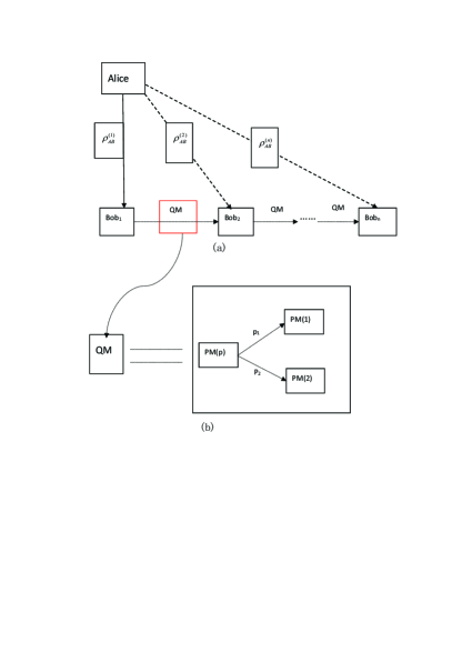
Figure 1: (a) A quantum state $\rho_{AB}^{(1)}$ is initially shared by Alice and Bob₍₁₎. Bob₍₁₎ performs some kind of quantum measurements on his part and then passes it to Bob₍₂₎. The post-measurement state is $\rho_{AB}^{(2)}$. Bob₍₂₎ measures $\rho_{AB}^{(2)}$ on his part and passes it to Bob₍₃₎ and so on. (b) Quantum measurement (QM) given by a random combination of several projective measurements (PMs) with different probabilities $p$. Before the experiment begins, all the parties agree to share correlated strings of classical data $p=\{p_{i}\}$ satisfying $\sum_{i}p_{i}=1$.

The high-dimensional quantum systems can carry more information and are more resistant to noises. High-dimensional quantum systems are important in improving the performance of quantum networks, quantum key distribution, quantum teleportation and quantum internet mkue ; sdrh ; mmaz ; hkrb . Therefore, in this article we study the nonlocal correlation sharing scenario for arbitrary high dimensional bipartite entangled pure states along the line of asat (Fig. 1). We show that projective measurement is also a sufficient condition for two observers to share the Bell nonlocality of any arbitrary dimensional bipartite entangled pure states.

II Nonlocal sharing of bipartite high-dimensional pure state

Let $H_{A}$ and $H_{B}$ be Hilbert spaces with dimensions $dim(H_{A})=s$ and $dim(H_{B})=t$, respectively (without loss of generality, we assume $s\leq t$). A bipartite pure state $|\psi\rangle\in H_{A}\otimes H_{B}$ has the Schmidt decomposition form, $|\psi\rangle=\sum_{i=1}^{s}c_{i}|i_{A}\rangle|i_{B}\rangle$, where $c_{i}\in[0,1]$, $\sum_{i=1}^{s}c_{i}^{2}=1$, $\{i_{A}\}_{1}^{s}$ and $\{i_{B}\}_{1}^{t}$ are the orthonormal bases of $H_{A}$ and $H_{B}$, respectively. $|\psi\rangle$ is entangled if and only if at least two $c_{i}$s are nonzero. Without loss of generality, below we assume that $c_{i}$ are arranged in descending order.

We focus on the sequential scenario shown in Fig. 1. To begin with, Alice and Bob₁ share an arbitrary entangled bipartite pure state $\rho_{AB}^{(1)}=|\psi\rangle\langle\psi|$. Bob_k $(k=1,2,\cdots,n)$ are restricted to perform two different projective measurement settings: PM(1) both choose projection measurement ($\lambda=1$)and PM(2) one chooses projection measurement, the other chooses identity operator ($\lambda=2$). Denote the binary input and output of Alice (Bob_k) by $X$ $(Y^{k})\in\{0,1\}$ and $A$ $(B^{(k)})\in\{0,1\}$, respectively. Before the experiment begins, all the parties agree to share the correlated strings of classical data $\lambda$ subjected to probability distribution $\{p_{\lambda}\}_{\lambda=1,2}$. Suppose Bob₁ performs the measurement according to $Y^{1}=y$ with outcome $B^{1}=b$. Averaged over the inputs and outputs of Bob₁, the unnormalized state shared between Alice and Bob₂ is given by

$$\rho_{AB}^{(2,\lambda)}=\frac{1}{2}\Sigma_{b,y}(I_{s}\otimes\sqrt{B_{b|y}^{(1,\lambda)}})\rho_{AB}^{(1)}(I_{s}\otimes\sqrt{B_{b|y}^{(1,\lambda)}}),$$ (1)

where $B^{(1,\lambda)}_{b|y}$ $(\lambda=1,2$) is the projective measurement ($(B^{(1,\lambda)}_{b|y})^{2}=B^{(1,\lambda)}_{b|y}$) corresponding to outcome $b$ of Bob^(1,λ)’s measurement for input $y$, $I_{s}$ is the $s\times s$ identity matrix. Repeating this process, one gets the state $\rho_{AB}^{(k,\lambda)}$ shared between Alice and Bob^(k), $k=2,3,\cdots,n$.

The Bell nonlocality is verified by the violation of the CHSH inequality jmar . Each pair Alice-Bob_k tests the CHSH inequality,

$$S_{k}\equiv\sum_{\lambda=1}^{2}p_{\lambda}S_{k}^{\lambda}\leq 2,$$ (2)

where

$$S_{k}^{\lambda}\equiv\sum_{x,y}(-1)^{xy}Tr(A_{x}\otimes B_{y}^{(k,\lambda)})\rho_{AB}^{(k,\lambda)}.$$ (3)

Here, $\{A_{x},B_{y}^{(k,\lambda)}\}_{k=1,2,\cdots}$ denote the observables of respective parties conditioned on $\lambda$. Only when $k=1$, $\rho_{AB}^{(1,\lambda)}=\rho_{AB}^{(1)}$.

Let us consider the simplest scenario, namely, $n=2$ and $s,t$ are even. We set the Alice’s quantum measurements to be given by observables

$$A_{0}=I_{\frac{s}{2}}\otimes(\cos\theta\sigma_{3}+\sin\theta\sigma_{1}),$$ (4)

and

$$A_{1}=I_{\frac{s}{2}}\otimes(\cos\theta\sigma_{3}-\sin\theta\sigma_{1})$$ (5)

for some $\theta\in[0,\frac{\pi}{2}]$.

Case (i): ($\lambda=1$). We set the Bob₁’s projective measurements to be given by observables

$$B_{0|0}^{(1,1)}=\frac{1}{2}[I_{t}+(I_{\frac{t}{2}}\otimes\sigma_{3})]$$ (6)

and

$$B_{0|1}^{(1,1)}=\frac{1}{2}[I_{t}+(I_{\frac{t}{2}}\otimes\sigma_{1})].$$ (7)

Denote $B_{1|y}^{(1,1)}=I_{t}-B_{0|y}^{(1,1)}$ and $B_{y}^{(1,1)}=B_{0|y}^{(1,1)}-B_{1|y}^{(1,1)}$ for $y=0,1$. Similar to the calculations in Ref. ztfs , it is not difficult to obtain that $S_{1}^{1}\geq 2(\cos\theta+K\sin\theta):=\mathaccent 866{S_{1}^{1}}$, where $K=2(c_{1}c_{2}+c_{3}c_{4}+\cdots+c_{s-1}c_{s})$, $0<K\leq 1$.

Using Eq.(1), we obtain

$$\rho_{AB}^{(2,1)}=\frac{1}{2}\rho_{AB}^{(1)}$$

$$+\frac{1}{4}[I_{s}\otimes(I_{\frac{t}{2}}\otimes\sigma_{3})]\rho_{AB}^{(1)}[I_{s}\otimes(I_{\frac{t}{2}}\otimes\sigma_{3})]$$

$$+\frac{1}{4}[I_{s}\otimes(I_{\frac{t}{2}}\otimes\sigma_{1})]\rho_{AB}^{(1)}[I_{s}\otimes(I_{\frac{t}{2}}\otimes\sigma_{1})].$$ (8)

Then taking $B_{y}^{(2,1)}=B_{y}^{(1,1)}$ for $y=0,1$, we get $S_{2}^{1}\geq(\cos\theta+K\sin\theta):=\mathaccent 866{S_{1}^{1}}$. The trade-off relationship between $\mathaccent 866{S_{1}^{1}}$ and $\mathaccent 866{S_{2}^{1}}$ is given by

$$\mathaccent 866{S_{2}^{1}}=\frac{1}{2}\mathaccent 866{S_{1}^{1}}.$$ (9)

When $\theta=\arctan K$, $\mathaccent 866{S_{1}^{1}}\$attains the maximum value $2\sqrt{1+K^{2}}$. At this moment $\mathaccent 866{S_{2}^{1}}=\sqrt{1+K^{2}}$. Moreover, when $|\psi\rangle=\frac{1}{\sqrt{2}}(|00\rangle+|11\rangle)$, that is, $K=1$, we obtain the same maximum value of $\mathaccent 866{S_{1}^{1}}$ as in Ref.asat .

Case (ii): ($\lambda=2$). We take the Bob₁’s projective measurements to be

$$B_{0|0}^{(1,2)}=I_{t}$$ (10)

and

$$B_{0|1}^{(1,2)}=\frac{1}{2}(I_{t}+(I_{\frac{t}{2}}\otimes\sigma_{1})).$$ (11)

Denote $B_{1|y}^{(1,2)}=I_{t}-B_{0|y}^{(1,2)}$ and $B_{y}^{(1,2)}=B_{0|y}^{(1,2)}-B_{1|y}^{(1,2)}$ for $y=0,1$. Similarly, we can obtain $S_{1}^{2}\geq 2K\sin\theta:=\mathaccent 866{S_{1}^{2}}$. By calculation, we have

$$\rho_{AB}^{(2,2)}=\frac{3}{4}\rho_{AB}^{(1)}$$

$$+\frac{1}{4}[I_{s}\otimes(I_{\frac{t}{2}}\otimes\sigma_{1})]\rho_{AB}^{(1)}[I_{s}\otimes(I_{\frac{t}{2}}\otimes\sigma_{1})].$$ (12)

Then take $B_{0}^{(2,2)}=I_{\frac{t}{2}}\otimes\sigma_{3}$, $B_{1}^{(2,2)}=I_{\frac{t}{2}}\otimes\sigma_{1}$, we obtain $S_{2}^{2}\geq 2K\sin\theta+\cos\theta:=\mathaccent 866{S_{2}^{2}}$. The trade-off relationship between $\mathaccent 866{S_{1}^{2}}$ and $\mathaccent 866{S_{2}^{2}}$ becomes

$$\mathaccent 866{S_{2}^{2}}=\mathaccent 866{S_{1}^{2}}+\frac{1}{2K}\sqrt{4K^{2}-(\mathaccent 866{S_{1}^{2}})^{2}}.$$ (13)

When $\theta=\arctan 2K$, $\mathaccent 866{S_{2}^{2}}$ achieves the maximum value $\sqrt{4K^{2}+1}$. Meanwhile, $\mathaccent 866{S_{1}^{2}}=\frac{4K^{2}}{\sqrt{4K^{2}+1}}$. In particular, for $|\psi\rangle=\frac{1}{\sqrt{2}}(|00\rangle+|11\rangle)$ ($K=1$), our the trade-off relation Eq. (13) gives rise to the Eq.(6) of Ref.asat .

Concerning the Bell nolocality, we assume that the probability of choosing the first (second) measurement is $p$ ($1-p$). According to the definition (2), it can be seen that $S_{1}=pS_{1}^{1}+(1-p)S_{1}^{2}\geq p\mathaccent 866{S_{1}^{1}}+(1-p)\mathaccent 866{S_{1}^{2}}=2p\sqrt{1+K^{2}}+(1-p)\frac{4K^{2}}{\sqrt{4K^{2}+1}}$ and $S_{2}=pS_{2}^{1}+(1-p)S_{2}^{2}\geq p\mathaccent 866{S_{2}^{1}}+(1-p)\mathaccent 866{S_{2}^{2}}=p\sqrt{1+K^{2}}+(1-p)\sqrt{4K^{2}+1}$. The nonlocality sharing problem is then transformed to find parameters $p$ and $K$ such that $S_{1}$ and $S_{2}$ are both greater than $2$. As long as the right-hand formulas of the two inequalities above are both greater than 2 is sufficient. From FIG.2 and FIG.3 we see that they can both be greater than $2$ for some $p$ and $K$. For example when $K=1$, $p\in[\frac{2\sqrt{5}-4}{2\sqrt{10}-4},\frac{\sqrt{5}-2}{\sqrt{5}-\sqrt{2}}]\approx[0.203,0.286]$, $S_{1}$ and $S_{2}$ are simultaneously greater than 2. Because $S_{1}$ and $S_{2}$ are both continuous functions of $p$ and $K$, there is still a finite domain in which $S_{1}$ and $S_{2}$ are both greater than $2$. This also fully demonstrates that projective measurements are sufficient for sharing Bell nonlocality for bipartite high dimension pure states.

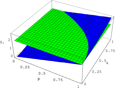
Figure 2: $p$ and $K$ as parameters of $S_{1}$ (blue), contour surface $S_{1}=2$ (green).

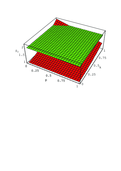
Figure 3: $p$ and $K$ as parameters of $S_{2}$ (red), contour surface $S_{2}=2$ (green).

When $s$ and $t$ are odd numbers, we only need to take the following measurement operators and follow the calculation method in Ref.ztfs to obtain the same conclusion as when $s$ is even, except that the expression of $K$ is changed to be $2(c_{1}c_{2}+c_{3}c_{4}+\cdots+c_{s-2}c_{s-1})$. The measurement operators can be selected as

$$A_{0}=\left(\begin{array}[]{cc}I_{[\frac{s}{2}]}\otimes(\cos\theta\sigma_{3}+\sin\theta\sigma_{1})&0\\ 0&1\end{array}\right)$$ (14)

and

$$A_{1}=\left(\begin{array}[]{cc}I_{[\frac{s}{2}]}\otimes(\cos\theta\sigma_{3}-\sin\theta\sigma_{1})&0\\ 0&1\end{array}\right)$$ (15)

for some $\theta\in[0,\frac{\pi}{2}]$, where $[m]$ represents the integer less or equal to $m$.

Similarly, in case (i) the corresponding projective measurements of Bob₁ are taken as

$$B^{(1,1)}_{0|0}=\frac{1}{2}[I_{t}+\left(\begin{array}[]{cc}(I_{[\frac{t}{2}]}\otimes\sigma_{3})&0\\ 0&1\end{array}\right)];$$

$$B^{(1,1)}_{0|1}=\frac{1}{2}[I_{t}+\left(\begin{array}[]{cc}(I_{[\frac{t}{2}]}\otimes\sigma_{1})&0\\ 0&1\end{array}\right)].$$

In case (ii), the corresponding projective measurements of Bob₁ are taken as

$$B^{(1,2)}_{0|0}=I_{t};$$

$$B^{(1,2)}_{0|1}=\frac{1}{2}[I_{t}+\left(\begin{array}[]{cc}(I_{[\frac{t}{2}]}\otimes\sigma_{1})&0\\ 0&1\end{array}\right)].$$

The corresponding projective measurements of Bob₂ are taken as

$$B_{0}^{(2,2)}=\left(\begin{array}[]{cc}(I_{[\frac{t}{2}]}\otimes\sigma_{3}&0\\ 0&1\end{array}\right);$$

$$B_{1}^{(2,2)}=\left(\begin{array}[]{cc}(I_{[\frac{t}{2}]}\otimes\sigma_{1}&0\\ 0&1\end{array}\right).$$

One derives again that the Bell nonlocality of bipartite high dimension pure states can be shared under projective measurements.

III Conclusions and Outlook

We have shown that projective measurements are sufficient for sharing the Bell nonlocality of high-dimensional entangled pure states. Namely, two independent Bobs may share states with a single Alice such that all the shared states violate the CHSH inequality. Our work greatly expands the range of quantum states given in Ref.asat . These quantum states share the Bell nonlocality through projection measurements and the distribution of shared classical randomness. These results are not only theoretically interesting, but also are of significance for experimental implementation, since Projective measurements enable one to demonstrate sequential nonlocality sharing in much simpler setups than previous non-projective measurementsmlmg ; mzxc ; glam ; tcym ; gmmh . In fact, unsharp quantum measurements have been proven to be useful for device-independent self-testing and recycling quantum communicationknab ; mjjm ; prap . Our results show that with only projection measurements it might be feasible for some sequential quantum information protocols related to quantum coherencesasm , entanglement witnessingasau ; adaa , quantum steeringsdsa ; xhxy and quantum contextualityhnrs .

We have proven that based on POVMs a high-dimension bipartite entangled pure state may produces $n$ sequential violations of the CHSH inequalityztfs . For projective measurements it is still unknown about how many sequence violations can occur for high-dimensional entangled pure states at most. It is also a meaningful problem to design the optimal projection measurement scheme. Instead of pure states, one may ask if any special mixed states can also be used for nonlocality sharing under projection measurements and shared randomness. Moreover, conclusions about simultaneous bilateral measurements and shared randomness would be also of importance.

Acknowledgments: We thank the anonymous reviewers for their helpful suggestions. This work is supported by the National Natural Science Foundation of China (NSFC) under Grant Nos.12204137, 12075159 and 12171044; the Hainan Provincial Natural Science Foundation of China under Grant No.121RC539, the specific research fund of the Innovation Platform for Academicians of Hainan Province under Grant No.YSPTZX202215, Beijing Natural Science Foundation (Grant No.Z190005).

References

- (1) N. Brunner, D. Cavalcanti, S. Pironio, V. Scarani, and S. Wehner, Rev. Mod. Phys. 86, 419 (2014).
- (2) J. Barrett, L. Hardy, and A. Kent, Phys. Rev. Lett. 95, 010503 (2005).
- (3) W.Z. Liu, Y. Z. Zhang, Y. Z. Zhen, M. H. Li, Y. Liu, J. Y. Fan, F. H. Xu, Q. Zhang, and J. W. Pan, Phys. Rev. Lett. 129, 050502 (2022).
- (4) Z. T. Qi, Y. H. Li, Y. W Huang, J. Feng, Y. L. Zheng, and X. F Chen, Light Sci. Appl. 10, 183 (2021).
- (5) Y. B. Sheng, L. Zhou, and G. L. Long, Sci. Bull. 67, 367 (2022).
- (6) H. Buhrman, R. Cleve, S. Massar, and R. de Wolf, Rev. Mod. Phys. 82, 665 (2010).
- (7) J. Ho, G. Moreno, S. Brito, F. Graffitti, C. L. Morrison, R. Nery, A. Pickston, M. Proietti, R. Rabelo, A. Fedrizzi, and R. Chaves, npj Quantum. Inf. 8, 13 (2022).
- (8) R. Silva, N. Gisin, Y. Guryanova, and S. Popescu, Phys. Rev. Lett. 114, 250401 (2015).
- (9) S. Mal, A. Majumdar, and D. Home, Mathematics 4, 48 (2016).
- (10) M. Schiavon, L. Calderaro, M. Pittaluga, G. Vallone, and P. Villoresi, Quantum Sci. Technol. 2, 015010 (2017).
- (11) M. J. Hu, Z. Y. Zhou, X. M. Hu, C. F. Li, G. C. Guo, and Y. S. Zhang, npj Quantum Inform. 4, 1 (2018).
- (12) A. Shenoy H., S. Designolle, F. Hirsch, R. Silva, N. Gisin, and N. Brunner, Phys. Rev. A 99, 022317 (2019).
- (13) D. Das, A. Ghosal, S. Sasmal, S. Mal, and A. S. Majumdar, Phys. Rev. A 99, 022305 (2019).
- (14) C. Ren, T. Feng, D. Yao, H. Shi, J. Chen, and X. Zhou, Phys. Rev. A 100, 052121(2019).
- (15) A. Kumari and A. K. Pan, Phys. Rev. A 100, 062130 (2019).
- (16) S. Saha, D. Das, S. Sasmal, D. Sarkar, K. Mukherjee, A. Roy, and S. S. Bhattacharya, Quantum Inf. Process. 18, 42 (2019).
- (17) G. Foletto, L. Calderaro, A. Tavakoli, M. Schiavon, F. Picciariello, A. Cabello, P. Villoresi, and G. Vallone, Phys. Rev. Applied 13, 044008 (2020)
- (18) T. F. Feng, C. L. Ren, Y. L. Tian, M. L. Luo, H. F. Shi, J. L. Chen, and X. Q. Zhou, Phys. Rev. A 102, 032220 (2020).
- (19) P. J. Brown and R. Colbeck, Phys. Rev. Lett. 125, 090401 (2020).
- (20) T. Zhang and S. M. Fei, Phys. Rev. A 103, 032216 (2021).
- (21) G. Foletto, M. Padovan, M. Avesani, H. Tebyanian, P. Villoresi, and G. Vallone, Phys. Rev. A 103, 062206 (2021).
- (22) S. Mukherjee and A. K. Pan, Phys. Rev. A 104, 062214 (2021).
- (23) S. Cheng, L. Liu, T. J. Baker, M. J. W. Hall, Phys. Rev. A 104, L060201 (2021).
- (24) S. Cheng, L. Liu, T. J. Baker, M. J. W. Hall, Phys. Rev. A 105, 022411 (2022).
- (25) C. Ren, X. Liu, W. Hou, T. Feng, and X. Zhou Phys. Rev. A 105, 052221 (2022).
- (26) T. Zhang, Q. Luo and X. Huang, Quantum Inf. Process. 21, 350 (2022).
- (27) S.S. Mahato and A.K. Pan, Phys. Rev. A 106, 042218 (2022)
- (28) J.H. Wang, Y.J. Wang, L.J. Wang, and Q. Chen, Phys. Rev. A 106, 052412 (2022).
- (29) M.L. Hu, J.R. Wang and H. Fan, Sci. China Phys. Mech. Astron. 65, 260312 (2022).
- (30) A. Steffinlongo and A. Tavakoli, Phys. Rev. Lett. 129, 230402 (2022).
- (31) Y. Xiao, Y.X. Rong, X.H. Han, S. Wang, X. Fan, W.C. Li, and Y.J. Gu, arXiv:2212.03815v1 [quant-ph](2022).
- (32) S.S. Abhyoudai, S. Mukherjee, and A. K. Pan, Phys. Rev. A 107, 012411(2023).
- (33) Y.L. Mao, Z.D. Li, A. Steffinlongo, B. Guo, B. Liu, S. Xu, N. Gisin, A. Tavakoli and J. Fan, Phys. Rev. Research 5, 013104 (2023).
- (34) T. Zhang, N. Jing, and S.M. Fei, Fron. Phys. 18, 31302 (2023).
- (35) Y. Xi, M.S. Li, L. Fu, and Z.J. Zheng, Phys. Rev. A 107, 062419 (2023).
- (36) M. Kues, et al. Nature 546, 622 (2017).
- (37) S. Wehner, D. Elkouss, R. Hanson, Science 362, 6412, (2018).
- (38) M. Erhard, M. Krenn and A. Zeilinger, Nat. Rev. Phys. 2, 365 (2022).
- (39) H.H. Lu, K.V. Myilswamy, R.S. Bennink, et al. Nat. Commun. 13, 4338 (2022).
- (40) J. F. Clauser, M. A. Horne, A. Shimony, and R. A. Holt, Phys. Rev. Lett. 23, 880 (1969).
- (41) K. Mohan, A. Tavakoli and N. Brunner, New J. Phys. 21, 083034 (2019).
- (42) N. Miklin, J. J. Borkala, and M. Pawlowski, Phys. Rev. Res. 2, 033014 (2020).
- (43) P. Roy and A.K. Pan, New J. Phys. 25, 013040 (2023).
- (44) S. Datta, and A. S. Majumdar, Phys. Rev. A 98, 042311 (2018).
- (45) A. Bera, S. Mal, A. Sen(De), and U. Sen, Phys. Rev. A 98, 062304 (2018).
- (46) A. G. Maity, D. Das, A. Ghosal, A. Roy, and A. S. Majumdar, Phys. Rev. A 101, 042340 (2020).
- (47) S. Sasmal, D. Das, S. Mal, and A. S. Majumdar, Phys. Rev. A 98, 012305 (2018).
- (48) X.H. Han, H.C. Qu, X. Fan, Y. Xiao, and Y.J. Gu, Phys. Rev. A 106, 042416 (2022).
- (49) H. Anwer, N. Wilson, R. Silva, S. Muhammad, A. Tavakoli, and M. Bourennane, Quantum 5, 551 (2021).