Nature of Topological Phase Transition of Kitaev Quantum Spin Liquids

Abstract

We investigate the nature of the topological quantum phase transition between the gapless and gapped Kitaev quantum spin liquid phases away from the exactly solvable point. The transition is driven by anisotropy of the Kitaev couplings. At the critical point the two Dirac points of the gapless Majorana modes merge, resulting in the formation of a semi-Dirac point with quadratic and linear band touching directions. We derive an effective Gross-Neveu-Yukawa type field theory that describes the topological phase transition in the presence of additional magnetic interactions. We obtain the infrared scaling form of the propagator of the dynamical Ising order parameter field and perform a renormalization-group analysis. The universality of the transition is found to be different to that of symmetry-breaking phase transitions of semi-Dirac electrons. However, as in the electronic case, the Majorana fermions acquire an anomalous dimension, indicative of the breakdown of the fractionalized quasiparticle description.

The spin-$1/2$ honeycomb Kitaev model [1] [Fig. 1(a)] has been at the forefront of research into quantum spin liquids (QSLs) [2, 3, 4] since it is exactly solvable after fractionalizing the spin operators into a set of Majorana fermions [1, 5, 6]. Some of these correspond to local bond excitations which are linked to $Z_{2}$ fluxes through the plaquettes of the honeycomb lattice. Since the fluxes are conserved, the Kitaev model can be diagonalized for each flux configuration, resulting in a non-interacting Hamiltonian for the remaining Majorana fermion species. In the ground state, zero-flux sector, this results in a Dirac dispersion identical to that of electrons in graphene.

Anisotropy of the Kitaev couplings can drive a topological phase transition from a gapless to a gapped $Z_{2}$ Kitaev QSL [1]. In the regime of large anisotropy, the latter can be mapped to the toric code model which exhibits anyonic excitations and plays an important role in the context of quantum computation and quantum error correction [7]. Approaching the topological phase transition from the gapless QSL side, the Dirac points of the gapless Majorana bands move along the edge of the Brillouin zone [Fig. 1(b)] and eventually merge, forming a semi Dirac point with a quadratic and a linear band touching direction. For larger anisotropies the spectrum becomes gapped. This behavior is very similar to the topological phase transition proposed to occur for electrons in strained honeycomb lattices [8, 9, 10] and was observed experimentally in black phosphorus [11, 12].

At first glance, the bond-directional exchange of the Kitaev model seems artificial, but it was realized that because of strong spin-orbital mixing [13, 14], the Kitaev model can be approximately realized in layered honeycomb iridates [15, 16, 17, 18, 19, 20, 21] and the halide $\alpha$-RuCl₃ [22, 23, 24]. Although in these materials the additional magnetic interactions are still slightly too large, leading to magnetic ordering at low temperatures, the experimental realization of a Kitaev QSL is certainly within reach.

In the presence of additional magnetic interactions, such as Heisenberg or Gamma couplings [3, 25], the model is no longer exactly solvable since the flux plaquette operators do not commute with the full Hamiltonian and the gapped Majorana modes, which correspond to flux excitations, acquire dynamics. While the selection of magnetically ordered states crucially depends on the nature of the additional couplings, the topological phase transition between the gapless and gapped Kitaev QSLs is expected to be universal.

In this Letter we analyze the nature of the topological quantum phase transition away from the exactly solvable point. To achieve this we perform a renormalization-group (RG) analysis of the effective Gross-Neveu-Yukawa (GNY) quantum field theory that describes the coupling of the dynamical Ising order parameter field to the gapless Majorana fermion semi-Dirac modes.

Instead of starting with the generic form of the effective field theory, we explicitly derive it for a specific microscopic model. Our starting point is the Kitaev model with couplings $K_{\gamma}>0$ along nearest-neighbour bonds $\langle i,j\rangle_{\gamma}$ ($\gamma=x,y,z$), perturbed by an antiferromagnetic nearest-neighbor Ising exchange $J>0$ [26, 27],

$$\hat{\cal H}=\sum_{\gamma=x,y,z}\sum_{\langle i,j\rangle_{\gamma}}K_{\gamma}\hat{\sigma}_{i}^{\gamma}\hat{\sigma}_{j}^{\gamma}+J\sum_{\langle i,j\rangle}\hat{\sigma}_{i}^{z}\hat{\sigma}_{j}^{z}.$$ (1)

Here the operators $\hat{\sigma}_{i}^{\gamma}$ denote spin-1/2 operators in units of $\hbar/2$, satisfying the spin-commutation algebra $[\hat{\sigma}_{i}^{\alpha},\hat{\sigma}_{j}^{\beta}]=2\delta_{ij}\epsilon_{\alpha\beta\gamma}\hat{\sigma}_{i}^{\gamma}$. In order to drive a topological phase transition, we allow for anisotropy $K_{z}>K_{x}=K_{y}=K$. For $J=0$, the topological phase transition is known to occur at $K_{z}/K=2$ [1].

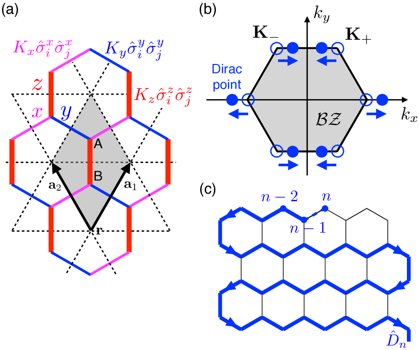
Figure 1: (a) Illustration of the bond-directional Ising exchanges $K_{\gamma}\hat{\sigma}_{i}^{\gamma}\hat{\sigma}_{j}^{\gamma}$ along the bonds $\gamma=x,y,z$ of the honeycomb Kitaev model. The unit cell contains two lattice sites ($A,B$) and is spanned by $\mathbf{a}_{1,2}=(\pm\frac{\sqrt{3}}{2},\frac{3}{2})$. (b) As a function of anisotropy $(K_{z}-K)/K$ the Dirac points of the gapless Majorana bands move along the edge of the Brillouin zone and merge at the topological phase transition between the gapless and gapped QSL states. (c) Snake string operator used for the two-dimensional Jordan-Wigner transformation.

We map this Kitaev-Ising model to a Hamiltonian in terms of spinless fermions, using a two-dimensional Jordan-Wigner transformation (JWT) with a string operator along the one-dimensional contour shown in Fig. 1(c). The mapping, which was used as an alternative way to obtain the exact solution of the pure Kitaev model [5], is defined as $\hat{\sigma}^{z}_{n}=1-2\hat{c}^{\dagger}_{n}\hat{c}_{n}=(\hat{c}^{\dagger}_{n}+\hat{c}_{n})(\hat{c}^{\dagger}_{n}-\hat{c}_{n})$, $\hat{\sigma}^{x}_{n}=\hat{D}_{n}(\hat{c}^{\dagger}_{n}+\hat{c}_{n})$ and $\hat{\sigma}^{y}_{n}=i\hat{D}_{n}(\hat{c}^{\dagger}_{n}-\hat{c}_{n})$. Here $n$ labels the position along the string and the string operator $\hat{D}_{n}=\prod_{\ell<n}(1-2\hat{c}^{\dagger}_{\ell}\hat{c}_{\ell})$ is required to match the spin commutation and fermion anti-commutation relations. The $x$ and $y$ bonds on the honeycomb lattice are nearest-neighbour bonds along the string. Although the coupling terms along these bonds involve spin components $\hat{\sigma}^{x}$ and $\hat{\sigma}^{y}$, the property $\hat{D}_{n}\hat{D}_{n+1}=1-2\hat{c}^{\dagger}_{n}\hat{c}_{n}$ ensures that the fermionized Hamiltonian remains local in the sense that no terms beyond nearest-neighbor coupling arise. The $z$ bonds connect spins that are not nearest neighbors along the snake string. As a result, any Hamiltonian that involves couplings between the $x$ or $y$ spin components along the $z$ bonds would become non-local. This however is not the case for the Kitaev Ising model (1).

In terms of Majorana fermions $\hat{\psi}_{A}(\mathbf{r})=i[\hat{c}^{\dagger}_{A}(\mathbf{r})-\hat{c}_{A}(\mathbf{r})]$, $\hat{\eta}_{A}(\mathbf{r})=\hat{c}^{\dagger}_{A}(\mathbf{r})+\hat{c}_{A}(\mathbf{r})$, $\hat{\psi}_{B}(\mathbf{r})=\hat{c}^{\dagger}_{B}(\mathbf{r})+\hat{c}_{B}(\mathbf{r})$ and $\hat{\eta}_{B}(\mathbf{r})=i[\hat{c}^{\dagger}_{B}(\mathbf{r})-\hat{c}_{B}(\mathbf{r})]$ the Hamiltonian is

$$\hat{\cal H} = -iK\sum_{\mathbf{r}}\sum_{i=1,2}\hat{\psi}_{A}(\mathbf{r})\hat{\psi}_{B}(\mathbf{r}+\mathbf{a}_{i})$$ (2)

$$+J\sum_{\mathbf{r}}\sum_{i=1,2}[i\hat{\psi}_{A}(\mathbf{r})\hat{\psi}_{B}(\mathbf{r}+\mathbf{a}_{i})]\;[i\hat{\eta}_{A}(\mathbf{r})\hat{\eta}_{B}(\mathbf{r}+\mathbf{a}_{i})]$$

$$+(K_{z}+J)\sum_{\mathbf{r}}[i\hat{\psi}_{A}(\mathbf{r})\hat{\psi}_{B}(\mathbf{r})]\;[i\hat{\eta}_{A}(\mathbf{r})\hat{\eta}_{B}(\mathbf{r})],$$

where $\{\hat{\psi}_{\alpha}(\mathbf{r}),\hat{\psi}_{\alpha^{\prime}}(\mathbf{r}^{\prime})\}=\{\hat{\eta}_{\alpha}(\mathbf{r}),\hat{\eta}_{\alpha^{\prime}}(\mathbf{r}^{\prime})\}=2\delta_{\alpha,\alpha^{\prime}}\delta_{\mathbf{r},\mathbf{r}^{\prime}}$ and $\{\hat{\psi}_{\alpha}(\mathbf{r}),\hat{\eta}_{\alpha^{\prime}}(\mathbf{r}^{\prime})\}=0$.

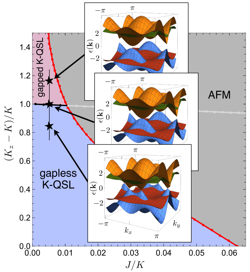
Figure 2: Mean-field phase diagram as a function of the anisotropy $(K_{z}-K)/K$ and the Ising exchange $J/K$. The evolution of the Majorana fermion spectrum across the topological phase transition between the gapless and gapped quantum spin liquid phases is shown in the insets.

Even for the pure Kitaev model, $J=0$, this seems to be an interacting problem. However, in this case the $\hat{\eta}$ Majorana fermions only live on isolated $z$ bonds and the bond operators $\hat{B}_{z}(\mathbf{r})=i\hat{\eta}_{A}(\mathbf{r})\hat{\eta}_{B}(\mathbf{r})$, which have eigenvalues $\pm 1$, commute with the Hamiltonian, $[\hat{B}_{z}(\mathbf{r}),\hat{\cal H}]=0$. In the absence of flux excitations we can replace all operators $\hat{B}_{z}(\mathbf{r})$ with the negative eigenvalue. This results in a non-interacting Hamiltonian for the $\hat{\psi}$ Majorana fermions with energy dispersion $\epsilon_{\psi,\pm}(\mathbf{k})=\pm|K_{z}+K(e^{i\mathbf{k}\cdot\mathbf{a}_{1}}+e^{i\mathbf{k}\cdot\mathbf{a}_{2}})|$. For $K_{z}/K<2$ we obtain gapless excitations with a pair of Dirac points. These merge at $K_{z}/K=2$ into a semi-Dirac point at $\mathbf{K}_{s}=(0,\frac{2\pi}{3})$. For $K_{z}/K>2$ the spectrum is gapped.

For non-zero $J$ the $\hat{\eta}$ Majorana fermions acquire dynamics and $[\hat{B}_{z}(\mathbf{r}),\hat{\cal H}]\neq 0$. In this case the model is no longer exactly solvable. An approximate phase diagram of the Kitaev-Ising model can be obtained using mean-field theory [27], where the bond expectation values $A_{\gamma}=\langle i\hat{\psi}_{A}(\mathbf{r})\hat{\psi}_{B}(\mathbf{r}+\bm{\delta}_{\gamma})\rangle$ and $B_{\gamma}=\langle i\hat{\eta}_{A}(\mathbf{r})\hat{\eta}_{B}(\mathbf{r}+\bm{\delta}_{\gamma})\rangle$ ($\bm{\delta}_{x}=\mathbf{a}_{1}$, $\bm{\delta}_{y}=\mathbf{a}_{2}$, $\bm{\delta}_{z}=\bm{0}$), as well as the staggered magnetization $m=\langle i\hat{\psi}_{A}(\mathbf{r})\hat{\eta}_{A}(\mathbf{r})\rangle=-\langle i\hat{\psi}_{B}(\mathbf{r})\hat{\eta}_{B}(\mathbf{r})\rangle$ are determined self-consistently. This results in the phase diagram shown in Fig. 2.

As expected, a relatively small Ising exchange $J$ leads to a first-order transition to an antiferromagnetic state. Importantly, a continuous topological phase transition between a gapless and a gapped Kitaev QSL still occurs for sufficiently small $J$. The insets of Fig. 2 show the evolution of the mean-field dispersion across this transition. While the gapless $\hat{\psi}$ Majorana modes behave in the same way as for the pure anisotropic Kitaev model, a key difference is that the gapped $\hat{\eta}$ modes become dispersive.

In order to understand the nature of the topological quantum phase transition, it is essential to include fluctuations beyond mean-field theory, arising from the interaction vertex. We recast the problem using a Grassmann path integral with action

$$S = \int_{k}\bm{\psi}^{\dagger}_{k}\left(\begin{array}[]{cc}-ik_{0}&-i\xi^{*}_{\mathbf{k}}\\ i\xi_{\mathbf{k}}&-ik_{0}\end{array}\right)\bm{\psi}_{k}+\int_{k}\bm{\eta}^{\dagger}_{k}\left(\begin{array}[]{cc}-ik_{0}&-i\lambda^{*}_{\mathbf{k}}\\ i\lambda_{\mathbf{k}}&-ik_{0}\end{array}\right)\bm{\eta}_{k}$$ (8)

$$+\sum_{\gamma}g_{\gamma}\sum_{\mathbf{r}}\int_{\tau}[i\psi_{A}(\mathbf{r},\tau)\psi_{B}(\mathbf{r}+\bm{\delta}_{\gamma},\tau)]$$

$$\times\;[i\eta_{A}(\mathbf{r},\tau)\eta_{B}(\mathbf{r}+\bm{\delta}_{\gamma},\tau)],$$

where $\tau$ denotes imaginary time, $\mathbf{k}$ the two-dimensional momentum, $k_{0}$ frequency, and $k=(k_{0},\mathbf{k})$. The complex functions $\xi_{\mathbf{k}}=\sum_{\gamma}a_{\gamma}e^{i\mathbf{k}\bm{\delta}_{\gamma}}$ and $\lambda_{\mathbf{k}}=\sum_{\gamma}b_{\gamma}e^{i\mathbf{k}\bm{\delta}_{\gamma}}$ are linked to the mean-field dispersions, $\epsilon_{\psi,\pm}(\mathbf{k})=\pm|\xi_{\mathbf{k}}|$ and $\epsilon_{\eta,\pm}(\mathbf{k})=\pm|\lambda_{\mathbf{k}}|$, respectively. We have written the interactions as $g_{\gamma}$, for brevity. Because of symmetry $g_{x}=g_{y}$, $a_{x}=a_{y}$ and $b_{x}=b_{y}$. Note that $b_{z}/b_{x,y}>2$ since the $\eta$ Majorana fermion bands are gapped.

As next step we integrate out the gapped Majorana modes $\eta$, which results in an effective interactions for the gapless $\psi$ Majorana fermions,

$$S_{\textrm{int}} = \sum_{\alpha\beta\gamma}\rho_{\alpha\beta}^{\gamma}\sum_{\mathbf{r}}\int_{\tau}[i\psi_{A}(\mathbf{r}-\bm{\delta}_{\alpha}+\bm{\delta}_{\gamma},\tau)\psi_{B}(\mathbf{r}+\bm{\delta}_{\gamma},\tau)]$$ (9)

$$\times\;[i\psi_{A}(\mathbf{r},\tau)\psi_{B}(\mathbf{r}+\bm{\delta}_{\beta},\tau)],$$

$$\rho_{\alpha\beta}^{\gamma} = \frac{1}{2}\sum_{\epsilon}g_{\alpha}g_{\beta}b_{\gamma}b_{\epsilon}\int_{q}\frac{e^{-i\mathbf{q}(\bm{\delta}_{\alpha}+\bm{\delta}_{\beta}-\bm{\delta}_{\gamma}-\bm{\delta}_{\epsilon})}}{(q_{0}^{2}+|\lambda_{\mathbf{q}}|^{2})^{2}},$$ (10)

with $\alpha\neq\gamma$ and $\beta\neq\gamma$. The different types of interactions $\rho_{\alpha\beta}^{\gamma}$ are visualized in Fig. 3 and correspond to the coupling of bond operators $\hat{A}_{\alpha}$ and $\hat{A}_{\beta}$ linked through a $\gamma$ bond.

It is important to stress that for $J=0$ we obtain $g_{x}=g_{y}=0$ and $b_{x}=b_{y}=0$ since interactions are restricted to the $z$ bonds and the $\eta$ bands are dispersionless. In this case all interactions $\rho_{\alpha\beta}^{\gamma}$ are equal to zero and we obtain a theory of non-interaction $\psi$ Majorana fermions.

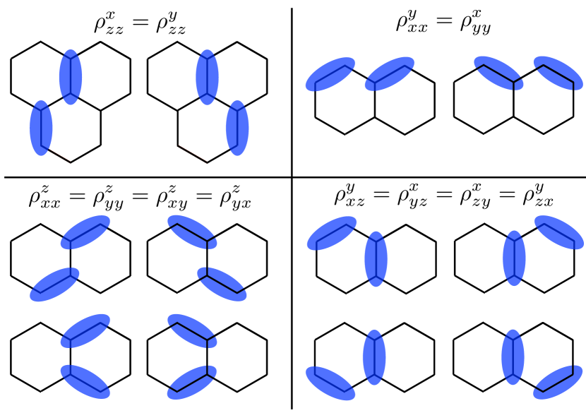
Figure 3: Illustration of the interaction terms between the bond-operators $\hat{A}_{ij}=i\hat{\psi}_{i}\hat{\psi}_{j}$ of the gapless Majorana modes $\hat{\psi}$, obtained after integrating the gapped modes $\hat{\eta}$.

As the final step we perform a Hubbard-Stratonovich decoupling of the interactions. For reasons that will become clear later, we only need to work out the coupling between the dynamical order-parameter field and the semi-Dirac Majorana fermions. The form of the coupling can be obtained more easily from a mean-field decoupling with $\phi_{\gamma}(\mathbf{r})=\langle i\hat{\psi}_{A}(\mathbf{r})\hat{\psi}_{B}(\mathbf{r}+\bm{\delta}_{\gamma})\rangle$. This results in $\sum_{\mathbf{r},\gamma}\Omega_{\gamma}(\mathbf{r})[i\hat{\psi}_{A}(\mathbf{r})\hat{\psi}_{B}(\mathbf{r}+\bm{\delta}_{\gamma})]$, where the fields $\Omega_{\gamma}(\mathbf{r})$ are certain combinations of $\phi_{\gamma}(\mathbf{r})$, e.g. $\Omega_{z}(\mathbf{r})=2(\rho_{zz}^{x}+\rho_{zz}^{y})\phi_{z}(\mathbf{r})+2\rho_{xz}^{y}\phi_{x}(\mathbf{r})+2\rho_{yz}^{x}\phi_{y}(\mathbf{r})$. After Fourier transform and expansion around the semi-Dirac point $\mathbf{K}_{s}=(0,\frac{2\pi}{3})$ we obtain the Yukawa coupling term of the low energy field theory,

$$S_{Y}[\phi,\bar{\bm{\psi}},\bm{\psi}]=\frac{g}{\sqrt{N}}\int_{k,q}\phi(q)\bar{\bm{\psi}}(k)\bm{\sigma}_{y}\bm{\psi}(k+q),$$ (11)

where $\bm{\sigma}_{y}$ denotes a Pauli matrix in sublattice space and the Ising fluctuation field is given by $\frac{g}{\sqrt{N}}\phi(q)=\Omega_{z}(q)-\Omega_{x}(q)-\Omega_{y}(q)$. Note that we generalized to $N$ flavours of semi-Dirac fermions and scaled the coupling accordingly. Expanding the quadratic part $S_{0}[\bar{\bm{\psi}},\bm{\psi}]$ of the action (8) around $\mathbf{K}_{s}$ we obtain

$$S_{0}[\bar{\bm{\psi}},\bm{\psi}]=\int_{k}\bar{\bm{\psi}}_{k}\left[-ik_{0}+k_{L}\bm{\sigma}_{x}+\left(k_{Q}^{2}+\Delta\right)\bm{\sigma}_{y}\right]\bm{\psi}_{k},$$ (12)

where $k_{L}=3ak_{y}$ and $k_{Q}=\frac{\sqrt{3a}}{2}q_{x}$ ($a=a_{x}=a_{y}$) are the rescaled momenta along the linear and quadratic directions, respectively and $\Delta=a_{z}-2a$ is the tuning parameter of the topological phase transition, where $\Delta=0$ at the critical point. As one might have anticipated, the dynamical bosonic fluctuation field $\phi(q)$ in $S_{Y}$ (11) couples in the same way as the static tuning parameter $\Delta$ in $S_{0}$ (12). The bosonic action $S[\phi]$ that is generated under perturbative RG is of the conventional Ginzburg-Landau form. However, this neglects the non-analytic bosonic self-energy correction $\Pi(q)$ due to the Landau damping of the order parameter fluctuations by gapless fermionic particle-hole fluctuations. Since $\Pi(q)$ dominates over the regular terms in the IR, it is crucial to use the quadratic bosonic action

$$S_{0}[\phi]=\int_{k}\phi(-k)G^{-1}_{\phi}(k)\phi(k)$$ (13)

with $G_{\phi}^{-1}(q)=\Pi(q)$ as starting point for subsequent perturbative RG calculation [28]. Using the correct infrared (IR) scaling form of the propagator, the fluctuation corrections under RG are independent of the choice of the ultraviolet (UV) cut-off scheme and therefore universal [29]. The bosonic self energy $\Pi(q)=g^{2}/N\int_{k}\text{Tr}\left[G_{\bm{\psi}}(k)\bm{\sigma}_{y}G_{\bm{\psi}}(k+q)\bm{\sigma}_{y}\right]$ is obtained by calculating the fermion polarization bubble digram [Fig. 4(a)] over the full range of frequencies and momenta where the non-analyticity arrises from the IR contribution ($k\to 0$). Unfortunately, for the case of semi-Dirac fermions this integral cannot be computed analytically. Following the procedure in Ref. [29], we obtain

$$\Pi(q)=\frac{g^{2}}{8\pi^{2}}\left|q_{Q}\right|F\left(\frac{q_{0}^{2}+q_{L}^{2}}{q_{Q}^{4}}\right),$$ (14)

where the function $F(u)$ for $u\in[0,\infty)$ is defined through the integral

$$F(u) = \int^{1}_{0}dt\int_{-\infty}^{\infty}dp$$ (15)

$$\times\left[\frac{(p+1)^{4}+p^{2}(p+1)^{2}+(1-t)u}{(p+1)^{4}t+p^{4}(1-t)+t(1+t)u}-2\right].\quad$$

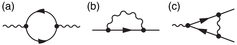
Figure 4: (a) Fermionic polarization bubble diagram that gives rise to the non-analytic IR propagator of the bosonic fluctuation field. Panels (b) and (c) show the diagram that contribute to the perturbative renormalization of the free-fermion action and the Yukawa coupling, respectively.

The field theory $S_{0}[\bar{\bm{\psi}},\bm{\psi}]+S_{0}[\phi]+S_{Y}[\phi,\bar{\bm{\psi}},\bm{\psi}]$ for the topological phase transition between the gapless and gapped Kitaev QSL states is very similar to the GNY theory that describes the quantum criticality of semi-Dirac fermions in 2+1 dimensions due to spontaneous symmetry breaking [29, 30, 31, 32, 33]. A key difference, however, is that for the symmetry-breaking transitions the Yukawa coupling is through the $\bm{\sigma}_{z}$ channel, which upon condensation of the order parameter results in the opening of a conventional mass gap in the fermion spectrum. The different form of the Yukawa coupling (11) through $\bm{\sigma}_{y}$ changes the form of the IR propagator $G_{\phi}(q)$ and of perturbative RG diagrams, resulting in distinct critical behavior.

To set up the RG calculation, we consider shells in frequency-momentum space, $\epsilon^{2}=k_{0}^{2}+k_{L}^{2}+k_{Q}^{4}$ with cut-off $\epsilon\leq\Lambda$ and integrate out modes from the infinitesimal shell $\Lambda e^{-d\ell}\leq\epsilon\leq\Lambda$, followed by a rescaling $k_{0}\to k_{0}e^{-d\ell}$, $k_{L}\to k_{L}e^{-d\ell}$ and $k_{Q}\to k_{Q}e^{-z_{Q}d\ell}$ to the old cut-off. Note that at tree-level $z_{Q}=1/2$. We further rescale the fields as $\psi\to\psi e^{-(\Delta_{\psi}/2)d\ell}$ and $\phi\to\phi e^{-(\Delta_{\phi}/2)d\ell}$.

The fermionic self energy correction $\bm{\Sigma}(k)d\ell=-g^{2}/N\int_{q}^{>}G_{\phi}(q)\bm{\sigma}_{y}G_{\bm{\psi}}(k+q)\bm{\sigma}_{y}$, which corresponds to the diagram in Fig. 4(b), is of the same form as the original kernel in $S_{0}[\bar{\bm{\psi}},\bm{\psi}]$,

$$\bm{\Sigma}(k)d\ell=\left[\Sigma_{0}(-ik_{0}\bm{\sigma}_{0}+k_{L}\bm{\sigma}_{x})+(\Sigma_{Q}k_{y}^{2}+\Sigma_{\Delta}\Delta)\bm{\sigma}_{y}\right]d\ell,$$ (16)

where the coefficients are evaluated as [34]

$$\Sigma_{0} = \frac{1}{2N}\int_{0}^{\infty}du\frac{1}{(u+1)^{2}F(u)}\approx\frac{0.1511}{N},$$ (17)

$$\Sigma_{Q} = -\frac{1}{2N}\int_{0}^{\infty}du\frac{u^{2}-12u+3}{(u+1)^{3}F(u)}\approx\frac{0.0163}{N},$$ (18)

$$\Sigma_{\Delta} = -\frac{1}{2N}\int_{0}^{\infty}du\frac{u-1}{(u+1)^{2}F(u)}\approx-\frac{0.4312}{N}.$$ (19)

From the diagram shown in Fig. 4(c) be obtain the correction $\Omega\bm{\sigma}_{y}d\ell=(g^{2}/N)\int_{q}^{>}G_{\phi}(q)\bm{\sigma}_{y}G_{\bm{\psi}}(q)\bm{\sigma}_{y}G_{\bm{\psi}}(q)\bm{\sigma}_{y}$ to the Yukawa coupling matrix, where the shell integral gives $\Omega=\Sigma_{\Delta}$.

$z_{Q}$	$\nu_{\Delta}^{-1}$	$\eta_{\bm{\psi}}$	$\eta_{\phi}$
$\frac{1}{2}-\frac{0.0674}{N}$	$1-\frac{0.5823}{N}$	$\frac{0.2185}{N}$	$-\frac{1.0298}{N}$

Table 1: Critical exponents for the topological phase transition between the gapless and gapped Kitaev QSL phases in (2+1) dimensions, calculated to one-loop order.

From the perturbative RG corrections we can extract critical exponents. Demanding that the fermion propagator at the transition ($\Delta=0$) remains scale invariant, we obtain the scaling exponent $z_{Q}=\frac{1}{2}+\frac{1}{2}\Sigma_{Q}-\frac{1}{2}\Sigma_{0}$ of the quadratic momentum direction $k_{Q}$ relative to the linear directions $k_{0}$ and $k_{L}$, and the scaling dimension $\Delta_{\bm{\psi}}=-\frac{7}{2}+\frac{3}{2}\Sigma_{0}-\frac{1}{2}\Sigma_{Q}=-\frac{7}{2}+\eta_{\bm{\psi}}$ of the Majorana fermion field, where $\eta_{\bm{\psi}}$ denotes the anomalous dimension. The correlation length exponent $\nu_{\Delta}$ of the topological phase transition is defined through the RG equation for $\Delta$, $\partial_{\ell}\Delta=(1-\Sigma_{0}+\Sigma_{\Delta})\Delta=\nu_{\Delta}^{-1}\Delta$. Finally, imposing that the Yukawa coupling $g$ remains scale invariant, we obtain the scaling dimension of the bosonic fluctuation field, $\Delta_{\phi}=-3+\eta_{\phi}$ with $\eta_{\phi}=2\Omega-\Sigma_{0}-\Sigma_{Q}$.

The resulting numerical values of the critical exponents are summarized in Table 1. For completeness, let us also investigate the relevance of the $\phi^{4}$ vertex at the topological phase transition. At tree-level, the scaling dimension of the coefficient is equal to $[\lambda]=-3(2+z_{Q})-2\Delta_{\phi}=-3/2$, demonstrating that the vertex is strongly irrelevant and hence can be neglected.

To summarize, we have derived the effective field theory for the topological quantum phase transition between the gapless and gapped Kitaev QSL phases. For the pure, exactly solvable Kitaev model the problem reduces to a free-fermion field theory. Away from the exactly solvable point, the field theory is of the GNY type and describes the coupling between an Ising fluctuation field to the gapless semi-Dirac Majorana fermion modes. We determined the critical exponents from an RG analysis and demonstrated that the universality of the topological phase transition is different to that describing symmetry-breaking phase transitions of semi-Dirac fermions.

The exponent $\nu_{\Delta}$ is linked to the opening of the energy gap in the Majorana fermion spectrum, $\Delta\sim(\delta-\delta_{c})^{\nu_{\Delta}}$, as well as to the separation of the Dirac points on the gapless QSL side, $(\delta k)\sim(\delta_{c}-\delta)^{\nu_{\Delta}/2}$. It could in principle be determined experimentally by measuring the evolution of the magnetic excitation continuum across the topological phase transition. However, it remains a challenge to realize the topological phase transition in experiment since uniaxial strain would not only affect the anisotropy of the Kitaev couplings but also distort the lattice, resulting in an increase of other magnetic exchange couplings.

The Kiteav QSL is a novel and exotic state of matter due to its long range entanglement and the fractionalization of spin degrees of freedom into Majorana fermions. Our work shows that the quantum criticality associated with a topological phase transition adds another layer of complexity. At the transition the emergent Majorana fermions acquire an anomalous dimension, indicative of a breakdown of the quasiparticle picture and the formation of a Majorana non-Fermi liquid state.