Inference on LATEs with covariates

Abstract

In theory, two-stage least squares (TSLS) identifies a weighted average of covariate-specific local average treatment effects (LATEs) from a saturated specification without making parametric assumptions on how available covariates enter the model. In practice, TSLS is severely biased when saturation leads to a number of control dummies that is of the same order of magnitude as the sample size, and the use of many, arguably weak, instruments. This paper derives asymptotically valid tests and confidence intervals for an estimand that identifies the weighted average of LATEs targeted by saturated TSLS, even when the number of control dummies and instrument interactions is large. The proposed inference procedure is robust against four key features of saturated economic data: treatment effect heterogeneity, covariates with rich support, weak identification strength, and conditional heteroskedasticity.

JEL codes: C12, C14, C21, C26.
Keywords: two-stage least squares, local average treatment effect, many controls, many instruments.

Introduction

With endogenous treatment and a binary instrument, Imbens and Angrist (1994) show that the two-stage least squares (TSLS) estimand has a causal interpretation as a local average treatment effect (LATE). Recently, Blandhol, Bonney, Mogstad, and Torgovitsky (2022) point out that the causal interpretation of the TSLS estimand is lost if we linearly include controls unless this is a correct parametric assumption. In the absence of a credible justification to linearly include the controls, Angrist and Imbens (1995) show that TSLS can consistently estimate a weighted average of LATEs provided that the number of possible values of the vector of controls is fixed: a researcher can select a saturated specification that includes (i) a dummy for each unique realized value of the vector of control variables and (ii) interactions of the instrument with these dummies. However, in most empirical settings the vector of controls has rich support, and saturated TSLS breaks down. As a result, applied work continuous to use the more parsimonious linear specification at the risk of targeting a non-causal estimand.

In this paper we propose a new method for inference in saturated specifications that do not require parametric assumptions even when the support of the controls is rich. More specifically, this method provides asymptotically valid tests and confidence intervals for an estimand that identifies the weighted average of LATEs targeted by saturated TSLS, allowing the number of control dummies and instrument interactions to be large. As saturated specifications contain only dummy variables, we can provide low-level assumptions for our results. The most important and rather mild assumption is that each covariate group contains at least two individuals for which the instrument is active and two for which the instrument is inactive. Settings with multiple or multivalued instruments also reduce to this setting as in that case dummies for each value of the instrument are interacted with the control dummies (Angrist and Imbens, 1995).

The proposed inference procedure is robust against four key features of saturated economic data: treatment effect heterogeneity, many control dummies and instrument interactions, weak identification strength, and conditional heteroskedasticity. While methods exist to address each of these features individually, we are the first to tackle their combination by building upon two recent advances in the literature. First, Chao, Swanson, and Woutersen (2023) propose an estimator for a homogeneous slope coefficient under many weak instruments in a panel data setting where fixed effects take the role of control dummies. We show that this estimator can consistently estimate a weighted average of LATEs in the setting of saturated instrumental variable estimation (SIVE). Second, in a setting with a fixed number of control dummies and instrument interactions, Kleibergen and Zhan (2021) propose a variance estimator for the score of the continuous updating objective function that is robust to treatment effect heterogeneity. While the SIVE estimator is very different from continuous updating, we use analogous ideas to formulate a heterogeneity robust variance estimator. We show that in the setting we consider, the assumptions in both papers can be relaxed to allow for the number of control dummies and instrument interactions to be asymptotically non-negligible relative to the sample size.

To highlight our contribution, we discuss the four features of the data we consider in turn. First, the inference method is robust to fully heterogeneous treatment effects. Imbens and Angrist (1994) focused attention on allowing for treatment effect heterogeneity in the estimation stage. In our setting with multiple instrument interactions, this heterogeneity is equally important in the inference stage as it affects the variance of the estimator. As such, we cannot use standard variance estimators for TSLS with multiple instruments, as they rely on the assumption of homogeneous treatment effects. A notable exception is the TSLS variance estimator proposed by Lee (2018), which however is not robust to the large number of instrument interactions in typical saturated specifications. We therefore propose a new variance estimator that is robust to treatment heterogeneity when the number of control dummies and instrument interactions are large.

Second, we allow for the number of control dummies and instrument interactions to be a non-negligible fraction of the sample size. To illustrate that this matters in practice, consider the four empirical examples studied by Blandhol et al. (2022): Table 1 shows the number of distinct covariate values and the sample size. We see that the number of covariate values, and hence the number of control dummies and instrument interactions in a saturated specification, is a substantial fraction of the sample size. The fact that TSLS is biased when the number of instruments grows proportionally with the sample size has been shown by Bekker (1994), and alternatives are provided by e.g. Hansen, Hausman, and Newey (2008); Ackerberg and Devereux (2009); Hausman, Newey, Woutersen, Chao, and Swanson (2012); Bekker and Crudu (2015). In addition to many instrument bias, Kolesár (2013) proposes estimators that also remove the bias due to many controls. However, inferential procedures based on these estimators have only been developed under the assumption that the number of control dummies is a negligible fraction of the sample size (Evdokimov and Kolesár, 2018).

Table 1: Empirical examples from Blandhol et al. (2022): sample size and covariate values

	Sample size	Covariate values	Ratio
Gelbach (2002)	440	186	0.42
Dube and Harish (2020)	107	11	0.10
Card (1995)	1780	238	0.13
Angrist and Krueger (1991)	329,463	659	0.002

Note: sample size is the effective sample size as reported in Blandhol et al. (2022) after accounting for perfect multicollinearity in the first stage. Covariates/Instruments indicates the number of distinct values of the available vector of controls, which equals the number of instrument interactions.

The third feature is that we accommodate weak instrument interactions. In particular, we allow the first stage signal to decrease to zero asymptotically. A saturated specification exacerbates the concern of weak identification, as even interacting a strong instrument with control dummies may result in instrument interactions that are only weakly related to the treatment. The condition that we impose on the identification strength has been shown by Mikusheva and Sun (2022) to be the weakest possible. While there is an extensive literature that combines the notion of many and weak instruments, e.g. Bekker and Kleibergen (2003); Chao and Swanson (2005); Hausman et al. (2012); Mikusheva and Sun (2022); Crudu et al. (2021); Matsushita and Otsu (2022); Lim et al. (2024), the focus has been on the linear IV model with a homogeneous slope coefficient.

The fourth feature is that the reduced form errors can be conditionally heteroskedastic. Inference in the presence of heteroskedasticity is non-trivial under many instruments and many controls as consistency results underlying the usual robust standard errors do not apply, see for instance Hausman, Newey, Woutersen, Chao, and Swanson (2012). Our newly proposed variance estimator employs estimators for the variances and covariances of the first stage and reduced form errors as in Hartley, Rao, and Kiefer (1969) to allow for heteroskedasticity. These variance estimators were also recently used by Cattaneo, Jansson, and Newey (2018). Compared to existing methods that allow for heteroskedasticity with many instruments, our newly proposed variance estimator is also robust to many control dummies and heterogeneous treatment effects.

Provided that the weighted average of covariate-specific LATEs as derived by Angrist and Imbens (1995) is a parameter of interest, this paper presents researchers with an inference framework that is readily applicable to many empirical instrumental variable estimation problems. Evidently, there are settings in which a researcher has a different causal parameter in mind. Słoczyński (2020) points out that in our parameter of interest a larger weight is placed on covariate groups with large variation in the instrument assignment and a strong first stage. Researchers that are concerned about this weighting, can use our identification robust methods to perform a subgroup-specific analysis that zooms in on groups with little variation in the instrument. Inference on subgroup-specific LATEs that are not weighted by the instrument strength may not provide much useful insights, as any unidentified LATE that receives nonzero weight will trigger the confidence interval to be the entire real line (Evdokimov and Lee, 2013).

We conduct a series of Monte Carlo simulations which set-up mimics key features of the data used in Card (1995), and has also been used by Blandhol et al. (2022). The results illustrate that the estimator we study is median unbiased for a range of values for the instrument strength and the number of covariate groups. Fully saturated TSLS and various jackknife estimators incur a bias that increases with the number of covariate groups and as the strength of the instrument decreases. A $t$-test using our proposed variance estimator yields close to nominal size control regardless of the instrument strength when the number of instruments is small. When the number of instruments increases, the test becomes progressively more conservative under weak instruments, while maintaining close to nominal size control under strong instruments. The standard $t$-test based on the fully saturated TSLS estimator with heteroskedasticity-robust standard errors shows large size distortions. The exception is the just-identified case where the control can take on only two values, in which TSLS is known to offer close to nominal size control even under weak instruments (Angrist and Kolesár, 2023). Finally, we verify numerically that not taking into account treatment heterogeneity when estimating the variance indeed leads to an oversized test. This underlines the importance of not only accounting for treatment effect heterogeneity in the estimation stage, which has been the main focus of the extant literature, but also in the inference stage.

To illustrate the estimator we briefly revisit the data used by Card (1995) in the specification selected by Słoczyński (2020). The goal of the study is to estimate the effect of going to college on income, where the endogenous decision of going to college is instrumented by the distance to college. In particular, we consider a specification with five binary controls and binarize the treatment to having some college attendance. We document that unrealistically large estimates are obtained when the covariate dummies are not interacted with the instruments. The estimator we study yields much more reasonable point estimates although the effects statistically cannot be distinguished from zero at conventional significance levels.

The remainder of this article is organized as follows. Section 2 explains the current practice of inferring LATEs with covariates from the data and its challenges. Section 3 introduces our proposed causal estimand and its inference procedure, supported by large sample theoretical results. Section 4 discusses the Monte Carlo simulations, Section 5 the empirical application, and Section 6 concludes.

LATEs with covariates

Suppose we are interested in the causal effect of a binary treatment $T_{i}$ on an outcome $Y_{i}$, for individuals $i=1,\dots,n$. For each individual, define the potential outcomes $Y_{i}(1)$ and $Y_{i}(0)$ corresponding to the values of $Y_{i}$ if individual $i$ is treated or not treated, respectively. Hence, the treatment effect is defined as $Y_{i}(1)-Y_{i}(0)$. The treatment is potentially endogenous and a binary instrument $Q_{i}$ and a vector of covariates $X_{i}$ is available to help identifying a causal effect. The developed theory applies equally well to the extensions to multivalued treatments and instruments in Angrist and Imbens (1995) as we discuss in Appendix B.

Define $\mathbb{X}=\{x_{1},\dots,x_{G}\}$ as the set of all possible $G$ unique realizations of $X_{i}$. Denote the potential treatment statuses $T_{i}(1)$ and $T_{i}(0)$ corresponding to the values of $T_{i}$ if individual $i$’s treatment assignment is given by $Q_{i}=1$ and $Q_{i}=0$, respectively. In case the outcome $Y_{i}$ also directly depends on $Q_{i}$, its corresponding potential outcomes are given by $Y_{i}(Q_{i},T_{i})$. If we condition on the covariates, the four instrumental variable assumptions in the Imbens and Angrist (1994) framework are the following.

Assumption 1

1. Independence: $(Y_{i}(q,t),T_{i}(q))\perp Q_{i}|X_{i}$ for $q\in\{0,1\}$ and $t\in\{0,1\}$,

2. Exclusion: $\mathbb{P}(Y_{i}(1,t)=Y_{i}(0,t)|X_{i})=1$ $a.s.$ for $t\in\{0,1\}$,

3. Relevance: $\mathbb{P}[T_{i}(1)\neq T_{i}(0)|X_{i}]>0$ $a.s.$,

4. Monotonicity: $\mathbb{P}[T_{i}(1)\geq T_{i}(0)|X_{i}]=1$ $a.s.$, or $\mathbb{P}[T_{i}(1)\leq T_{i}(0)|X_{i}]=1$ $a.s.$

These assumptions allow for complete treatment effect heterogeneity across all individuals, and do not impose any parametric assumptions. The monotonicity assumption is referred to in Blandhol et al. (2022) as weak monotonicity, because it allows the effect of the instrument on the treatment to have a different direction for each covariate group. Strong monotonicity requires $\mathbb{P}[T_{i}(1)\geq T_{i}(0)]=1$ or $\mathbb{P}[T_{i}(1)\leq T_{i}(0)]=1$, and therefore assumes that the effect of switching on the instrument on potential treatment status is (weakly) in the same direction for all individuals.

Within the LATE framework, causal effects are estimated of the form

$$\tau= \sum_{g}\omega(x_{g})\tau(x_{g})\text{ with }\sum_{g}\omega(x_{g})=1,\,\omega(x_{g})\geq 0\text{ for }g=1,\dots,G,\text{ and }$$ (1)

$$\tau(x_{g})= \mathbb{E}[Y_{i}(1)-Y_{i}(0)|T_{i}(1)\neq T_{i}(0),X_{i}=x_{g}].$$ (2)

The causal effect is then a positively weighted average of covariate-specific LATEs. The following well-known result shows that the covariate group specific LATEs $\tau(x_{g})$ are indeed identified.

Lemma 1

Assume that $\mathbb{E}[Y_{i}|Q_{i},X_{i}]$ is almost surely bounded. Under Assumption 1 it holds that

$$\frac{\mathbb{E}[Y_{i}|Q_{i}=1,X_{i}={x}_{g}]-\mathbb{E}[Y_{i}|Q_{i}=0,X_{i}={x}_{g}]}{\mathbb{E}[T_{i}|Q_{i}=1,X_{i}={x}_{g}]-\mathbb{E}[T_{i}|Q_{i}=0,X_{i}={x}_{g}]}=\tau(x_{g}).$$ (3)

This result is discussed in Angrist and Pischke (2009), among others. For completeness, we provide a short proof in Section C.1.

In practice, the number of observations in each covariate-group is usually small, and the moments in Lemma 1 cannot be accurately estimated. This provides a researcher with two options. First, we can maintain the focus on the LATE parameters, and use an (estimated) propensity score to aggregate the covariate specific LATEs. However, the propensity score can be difficult to estimate and limited overlap produces substantial statistical challenges. To avoid having to estimate the propensity score, an attractive option is to rely on regression to estimate a weighted average of the covariate group specific LATEs as the parameter of interest, where the weights are automatically selected through the regression model that is specified.

In this paper we focus on the regression approach. There are then several strategies for estimating the causal effect in (1). First, we can make a parametric assumption that restricts how the covariates enter the model. The default option is to include the covariates linearly in the first and second stage. Blandhol et al. (2022) shows that if this parametric assumption is incorrect, then TSLS has no causal interpretation.

To avoid parametric assumptions, a substantial and active literature considers semiparametric estimators (Abadie, 2003), or non-parametric estimators (Frölich, 2007). In particular, recent developments highlight the potential of machine learning techniques as non-parametric estimators for the effect of the controls on the outcome, endogenous treatment and instrumental variable, e.g. Chernozhukov et al. (2018). However, these algorithms need to attain a particular convergence rate, and it is not immediately clear whether the required conditions are met under weak identification (Mikusheva and Sun, 2023).

Finally, we can saturate the specification as suggested by Angrist and Imbens (1995). If we saturate, the two stage least squares estimator will only be consistent if the number of possible values of the covariate vector is fixed. However, say we have 10 binary controls, then this already gives us 1,024 possible values of the covariate vector. To accommodate cases with increasingly rich support of the covariates, we propose a new procedure that allows for reliable inference in saturated specifications. The only material additional assumption that we make is that in each covariate group there are at least two individuals for each value of the instrument.

Saturating the covariates

Angrist and Imbens (1995) show that $\tau$ can be estimated by TSLS in saturated specifications: the first stage includes dummies for each possible value of $X_{i}$ and a full set of interactions between these dummies and the instrument, and the second stage includes the treatment variable and the control dummies. By including dummies for each possible value of the covariates, no parametric assumptions are required. To be more precise, define the $G\times 1$ vector $W_{i}$ has elements $W_{ig}=\mathbbm{1}[X_{i}=x_{g}]$, indicating the covariate group of individual $i$. The $G\times 1$ vector $Z_{i}$ contains the instrument interactions $Z_{ig}=Q_{i}\mathbbm{1}[X_{i}=x_{g}]$. Note that $\sum_{g}W_{ig}=1$ and $\sum_{g}Z_{ig}=Q_{i}$. Define $n_{g}=\sum_{i}W_{ig}$ as the number of individuals in covariate group $g$, and $m_{g}=\sum_{i}Z_{ig}$ as the number of individuals in covariate group $g$ with an active instrument.

Both the full set of covariate group indicators and the full set of instrument interactions are required for nonparametric estimation of $\tau$ by TSLS (Blandhol et al., 2022). This ensures that the conditional expectation of the instrument given the covariate groups $\mathbb{E}[Q_{i}|X_{i}]$ is linear in the covariate group indicators. This allows for correctly partialling out the covariates, which otherwise may induce negative weights into $\tau$. Without the instrument interactions, the first stage does not necessarily reproduce the direction of the monotonicity assumption in all covariate groups. With a binary instrument, omitting the instrument interactions requires the direction of the monotonicity to be invariant to the covariate group.

It is clear that saturation can only work if we observe each covariate value more than once. Moreover, to achieve identification each covariate groups has to include both individuals with an active and an inactive instruments. The setup we consider, with many control dummies and many instrument interactions, requires the number of observations in each group to satisfy the following assumption.

Assumption 2

Group sizes: $m_{g}\geq 2$ and $n_{g}-m_{g}\geq 2$ for all $g=1,\dots,G$.

This assumption is rather mild. It requires that both the number of individuals with an active instrument and nonactive instrument has to be larger than one in each covariate group.

Estimation challenges

While saturation results in a causal TSLS estimand if the number of possible covariate values is small, it is not straightforward to find a causal estimand in the empirically more common setting in which the controls have rich support. Since each group requires an indicator, and the instrument is interacted with these indicators, this automatically results into a large set of control dummies and a large set of instruments. In this setting, TSLS is known to be biased, see e.g. Kolesár (2013).

Second, the instrument interactions may weaken the instrument strength. Instrument strength is measured by the first stage signal, which can be written as $\text{FS}=\sum_{g}\mathbb{P}[X_{i}=x_{g}]\pi(x_{g})^{2}\mathbb{V}[Q_{i}|X_{i}=x_{g}]$ with complier shares $\pi(x_{g})=\mathbb{P}[T_{i}(1)\neq T_{i}(0)|X_{i}=x_{g}]$ and treatment assignment variation $\mathbb{V}[Q_{i}|X_{i}=x_{g}]$. If the complier share and the variation in treatment assignment is homogeneous across covariate groups, that is $\pi(x_{g})=\pi$ and $\mathbb{V}[Q_{i}|X_{i}=x_{g}]=\mathbb{V}[Q_{i}]$, the strength of the instrument interactions $Z$ equals the strength of the instrument $Q$. However, in settings where the proportion of compliers is large in groups with a low number of treated or untreated units, while the proportion of compliers is small in groups with a number of treated units close to half of the number of group members, the first stage is likely weak. It is well known that under a large number of potentially weak instruments TSLS can be severely biased, see e.g. Bekker (1994) and Chao and Swanson (2005).

Two-stage least squares

Define the $n$-dimensional vectors $Y=(Y_{1},\ldots,Y_{n})^{\prime}$ and $T=(T_{1},\ldots,T_{n})^{\prime}$, and the $n\times G$-dimensional matrices $W=(W_{1}^{\prime},\ldots,W_{n}^{\prime})^{\prime}$ and $Z=(Z_{1}^{\prime},\ldots,Z_{n}^{\prime})^{\prime}$. Define the residual maker matrix $M_{W}=I_{n}-W(W^{\prime}W)^{-1}W^{\prime}$ with $I_{n}$ the $n$-dimensional identity matrix. The TSLS estimand is commonly defined as

$$\beta^{\text{TSLS}}=\frac{\mathbb{E}[T^{\prime}PY|Q,X]}{\mathbb{E}[T^{\prime}PT|Q,X]},$$ (4)

where $P=M_{W}Z(Z^{\prime}M_{W}Z)^{-1}Z^{\prime}M_{W}$ partials out the controls $W$ from the first stage and the second stage. However, this estimand is problematic when the number of covariate groups is large as the following result makes precise.

Lemma 2

Under Assumption 1 and 2 it holds that

$$\beta^{\emph{TSLS}}=\frac{\sum_{g}\tilde{\emph{P}}[X_{i}=x_{g}]\pi(x_{g})^{2}\tilde{\emph{V}}[Q_{i}|X_{i}=x_{g}]\tau(x_{g})+\frac{1}{n}\sum_{i}\mathbb{E}[u_{i}\varepsilon_{i}|Q_{i},X_{i}]P_{ii}}{\sum_{g}\tilde{\emph{P}}[X_{i}=x_{g}]\pi(x_{g})^{2}\tilde{\emph{V}}[Q_{i}|X_{i}=x_{g}]+\frac{1}{n}\sum_{i}\mathbb{E}[u_{i}^{2}|Q_{i},X_{i}]P_{ii}},$$ (5)

where $\tilde{\emph{P}}[X_{i}=x_{g}]=\frac{n_{g}}{n}$, $\pi(x_{g})=\emph{P}[T_{i}(1)\neq T_{i}(0)|X_{i}=x_{g}]$, $\tilde{\emph{V}}[Q_{i}|X_{i}=x_{g}]=\frac{m_{g}}{n_{g}}(1-\frac{m_{g}}{n_{g}})$, $u_{i}=T_{i}-\mathbb{E}[T_{i}|Q_{i},X_{i}]$, $\varepsilon_{i}=Y_{i}-\mathbb{E}[Y_{i}|Q_{i},X_{i}]$, and $P_{ii}=\sum_{g}\frac{1}{n_{g}}W_{ig}\frac{(Z_{ig}-\tilde{\emph{P}}[Q_{i}=1|X_{i}=x_{g}])^{2}}{\tilde{\emph{V}}[Q_{i}|X_{i}=x_{g}]}$.

A proof is deferred to Section C.2. Note that $\tilde{\text{P}}[X_{i}=x_{g}]$, $\tilde{\text{V}}[Q_{i}|X_{i}=x_{g}]$, and $\tilde{\text{P}}[Q_{i}=1|X_{i}=x_{g}]$ are the sample analogues of ${\mathbb{P}}[X_{i}=x_{g}]$, ${\mathbb{V}}[Q_{i}|X_{i}=x_{g}]$, and ${\mathbb{P}}[Q_{i}=1|X_{i}=x_{g}]$.

Lemma 2 shows that both the second term in the numerator and the second term in the denominator have to go to zero for $\beta^{\text{TSLS}}$ to identify $\tau$. In this case the weights in (1) equal $\omega^{\text{TSLS}}(x_{g})=\frac{\tilde{\emph{P}}[X_{i}=x_{g}]\pi(x_{g})^{2}\tilde{\emph{V}}[Q_{i}|X_{i}=x_{g}]}{\sum_{g}\tilde{\emph{P}}[X_{i}=x_{g}]\pi(x_{g})^{2}\tilde{\emph{V}}[Q_{i}|X_{i}=x_{g}]}$. It is clear that the additional terms go to zero when $P_{ii}$ is small. Some interpretation of this result can be obtained by noting that

$$P_{ii}=\sum_{g}W_{ig}\left(Z_{ig}\frac{1}{m_{g}}\frac{n_{g}-m_{g}}{n_{g}}+(1-Z_{ig})\frac{1}{n_{g}-m_{g}}\frac{m_{g}}{n_{g}}\right).$$ (6)

Hence, for TSLS to have a causal interpretation, in each covariate group the number of individuals for which the instrument is active ($m_{g}$) and the number of individuals for which the instrument is inactive ($n_{g}-m_{g}$) need to be large. This requirement becomes more stringent as the strength of the instrument interactions measured by $\sum_{g}\tilde{\emph{P}}[X_{i}=x_{g}]\pi(x_{g})^{2}\tilde{\emph{V}}[Q_{i}|X_{i}=x_{g}]$ decreases.

As we have seen in Table 1, the number of covariate groups is generally large and nonneglible relative to the number of individuals. In this case, at least a number of covariate groups has to have a small number of observations, and the additional terms in Lemma 2 do not go to zero. This bias is known as the many instrument bias of TSLS. Under homogenous treatment effects, and assuming homoskedastic errors, one can follow Bekker (1994) in using LIML to avoid this bias. However, Kolesár (2013) points out that with treatment effect heterogeneity, the estimand of LIML is generally not causal.

In Lemma 2 we condition both on the instrument and the covariates. This estimand can generally be more accurately inferred from the data relative to the unconditional counterpart. This point is made by Crump et al. (2009) in a regression context. In the IV context, Evdokimov and Kolesár (2018) show that both the conditional and unconditional estimands are a weighted combination of covariate specific LATEs, where the unconditional estimand integrates out sampling uncertainty in the combination weights. As such, confidence intervals for the unconditional estimand are wider. We focus on the conditional estimand in the subsequent analysis.

Jackknife instrumental variables estimation

It follows from Lemma 2 that the bias in TSLS is due to the diagonal elements $P_{ii}$. A frequently used approach to reduce many instrument bias is to employ a jackknife-style correction (Angrist, Imbens, and Krueger, 1999; Ackerberg and Devereux, 2009). In the current setting, we could remove the diagonal of $P$, denoted by $D_{P}$, to obtain an estimand referred to as the JIVE1,

$$\beta^{\text{JIVE1}}=\frac{\mathbb{E}[T^{\prime}(P-D_{P})Y|Q,X]}{\mathbb{E}[T^{\prime}(P-D_{P})T|Q,X]}.$$ (7)

This diagonal removal has been the basis of recent papers in the literature on identification-robust inference under many instrument sequences (Mikusheva and Sun, 2022; Crudu, Mellace, and Sándor, 2021; Matsushita and Otsu, 2022). It ensures that the many instrument bias present in TSLS disappears. However, in the present case it may nevertheless not be an attractive option. With a potentially large set of control variables, the consequence of removing the diagonal elements $P_{ii}$ is that the controls are no longer projected out. Indeed, the following result shows that removing the diagonal of the projection matrix biases the estimand.

Lemma 3

Under Assumption 1 and 2 it holds that

$$\beta^{\emph{JIVE1}}=\frac{\sum_{g}\tilde{\emph{P}}[X_{i}=x_{g}]\pi(x_{g})^{2}\tilde{\emph{V}}[Q_{i}|X_{i}=x_{g}](1-\tilde{\emph{P}}[Q_{i}=1,X_{i}=x_{g}])\tau(x_{g})-B_{Y}}{\sum_{g}\tilde{\emph{P}}[X_{i}=x_{g}]\pi(x_{g})^{2}\tilde{\emph{V}}[Q_{i}|X_{i}=x_{g}](1-\tilde{\emph{P}}[Q_{i}=1,X_{i}=x_{g}])-B_{T}},$$ (8)

where

$$B_{Y}= \sum_{g}\tilde{\emph{P}}[X_{i}=x_{g}]\pi(x_{g})(\phi_{g}+\tau(x_{g})\psi_{g})\tilde{\emph{V}}[Q_{i}|X_{i}=x_{g}]\tilde{\emph{P}}[Q_{i}=1,X_{i}=x_{g}]+\frac{1}{n}\psi_{g}\phi_{g},$$ (9)

$$B_{T}= 2\sum_{g}\tilde{\emph{P}}[X_{i}=x_{g}]\pi(x_{g})\psi_{g}\tilde{\emph{V}}[Q_{i}|X_{i}=x_{g}]\tilde{\emph{P}}[Q_{i}=1,X_{i}=x_{g}]+\frac{1}{n}\psi_{g}^{2},$$ (10)

with $\tilde{\emph{P}}[Q_{i}=1,X_{i}=x_{g}]=\frac{1}{m_{g}}$, $\psi_{g}=\mathbb{E}[T_{i}|Z_{ig}=0,W_{ig}=1]$, and $\phi_{g}=\mathbb{E}[Y_{i}|Z_{ig}=0,W_{ig}=1]$.

A proof is deferred to Section C.3. While removing the diagonal elements has removed the many instrument bias, this is done at a high cost. When the effect of the controls on the treatment and/or the outcome are large, as measured by $\phi_{g}$ and $\psi_{g}$, the estimand for JIVE1 can be substantially different from $\tau$ and seems difficult to interpret.

An alternative jackknife approach is to first partial out the controls before removing the diagonal. This gives the following estimand labeled JIVE2.

$$\beta^{\text{JIVE2}}=\frac{\mathbb{E}[T^{\prime}M_{W}(P-D_{P})M_{W}Y|Q,X]}{\mathbb{E}[T^{\prime}M_{W}(P-D_{P})M_{W}T|Q,X]}.$$ (11)

The following theorem shows that this in fact reintroduces the many instrument bias, although it is smaller than that in TSLS. Also, while the estimand differs from TSLS, the weights on the covariate specific LATEs continue to be positive.

Lemma 4

Under Assumption 1 and 2 it holds that

$$\beta^{\emph{JIVE2}}=\frac{\sum_{g}\tilde{\emph{P}}[X_{i}=x_{g}]\pi(x_{g})^{2}\tilde{\emph{V}}[Q_{i}|X_{i}=x_{g}]\tau(x_{g})+B_{Y,1}+B_{Y,2}}{\sum_{g}\tilde{\emph{P}}[X_{i}=x_{g}]\pi(x_{g})^{2}\tilde{\emph{V}}[Q_{i}|X_{i}=x_{g}]+B_{T,1}+B_{T,2}}$$ (12)

where

$$\begin{split}B_{Y,1}&=-\frac{1}{n}\sum_{g}\pi(x_{g})^{2}\left[1-3\tilde{\emph{V}}[Q_{i}|X_{i}=x_{g}]\right]\tau(x_{g}),\quad B_{Y,2}=\frac{1}{n}\sum_{i=1}^{n}\mathbb{E}[u_{i}\varepsilon_{i}|X_{i},Q_{i}]\left(\frac{2}{n_{g}}P_{ii}-\frac{1}{n_{g}^{2}}\right),\\ B_{T,1}&=-\frac{1}{n}\sum_{g}\pi(x_{g})^{2}\left[1-3\tilde{\emph{V}}[Q_{i}|X_{i}=x_{g}]\right],\quad B_{T,2}=\frac{1}{n}\sum_{i=1}^{n}\mathbb{E}[u_{i}^{2}|X_{i},Q_{i}]\left(\frac{2}{n_{g}}P_{ii}-\frac{1}{n_{g}^{2}}\right).\end{split}$$ (13)

The proof is similar as for Lemma 3 and omitted. In this case, the causal estimand still changes relative to TSLS, but under Assumption 2 the weights on $\tau(x_{g})$ will lie between 0 and the TSLS weights. When the noise terms are nonzero we see that the many instrument bias returns. To quantify this bias, consider momentarily a homoskedastic setting where $\mathbb{E}[u_{i}\varepsilon_{i}|X_{i},Q_{i}]=\sigma_{u\varepsilon}$. We see that $B_{Y,2}=\frac{\sigma_{u\varepsilon}}{n}\sum_{g=1}^{G}\frac{1}{n_{g}}$ compared to the bias in TSLS that is $\frac{\sigma_{u\varepsilon}}{n}\sum_{g=1}^{G}1$. We conclude that JIVE2 offers a substantial bias reduction, especially when $n_{g}$ is large. However, under many instruments, $n_{g}$ is fixed and the bias is of the same order as for TSLS.

Saturated instrumental variable estimation

A causal estimand

We now consider an estimand identical to that of TSLS when the number of possible values of the vector of controls is fixed, but that does not suffer from the many instrument bias when the number of covariate values grows. Define the matrix $V=[Z,W]$ consisting of the instrument interactions and the covariate group indicators, and define the residual maker matrix ${M}_{Z,W}=I-V(V^{\prime}V)^{-1}V^{\prime}$. The SIVE estimand is specified as

$$\beta^{\text{SIVE}}=\frac{\mathbb{E}[T^{\prime}(P-{M}_{Z,W}D{M}_{Z,W})Y|Q,X]}{\mathbb{E}[T^{\prime}(P-{M}_{Z,W}D{M}_{Z,W})T|Q,X]},$$ (14)

where $D$ is a diagonal matrix with diagonal elements such that $P_{ii}=[{M}_{Z,W}D{M}_{Z,W}]_{ii}$. It follows that (14) is a jacknife estimand, which removes the diagonal of $P$ and hence the bias in the TSLS estimand. At the same time, by pre- and post-multiplying $D$ by ${M}_{Z,W}$, the controls are projected out correctly and the bias in JIVE is prevented. In addition to the controls, ${M}_{Z,W}$ also projects out the instrument interactions, removing the bias in the TSLS estimand.

The SIVE estimator has been proposed by Chao, Swanson, and Woutersen (2023) as Fixed Effect Jackknife IV (FEJIV). They show that the diagonal elements of $D$ can be obtained by solving a system of linear equations with a unique solution, and derive consistency results in a linear instrumental variable regression with fixed effects using panel data with many weak instruments. Within our saturated setting, we can derive a closed-form expression for $D$, and show that the estimator identifies a weighted average of covariate-specific LATEs. These results require a different, but arguably weaker set of assumptions. For instance, we allow the number of control dummies and instrument interactions to be asymptotically non-negligible relative to the sample size, and Assumption 2 relaxes Assumption 6 in Chao et al. (2023) that requires $m_{g}\geq 3$ and $n_{g}-m_{g}\geq 3$.

The following result shows that the diagonal matrix $D$ in (14) exists under Assumption 2 and its elements are available in closed form.

Lemma 5

Under Assumption 2, it holds that if $D$ is a diagonal matrix with elements

$$D_{ii}=\sum_{g}\frac{1}{n_{g}}W_{ig}\left[\frac{n_{g}-m_{g}}{m_{g}-1}Z_{ig}+\frac{m_{g}}{n_{g}-m_{g}-1}(1-Z_{ig})\right]$$ (15)

then $P_{ii}=[{M}_{Z,W}D{M}_{Z,W}]_{ii}$ with $P=M_{W}Z(Z^{\prime}M_{W}Z)^{-1}Z^{\prime}M_{W}$ and $M_{W}=I_{n}-W(W^{\prime}W)^{-1}W^{\prime}$.

The proof is deferred to Section C.4. The result shows that when the number of covariate values is small and both $m_{g}$ and $n_{g}-m_{g}$ are large, the diagonal elements $D_{ii}$ are small and the estimator reduces to the TSLS estimator.

Because the term that is substracted in the numerator and denominator of (14) is orthogonal to the instruments and controls, it is straightforward to establish that the SIVE estimand has a causal interpretation that is identical to the unbiased TSLS estimand, without requiring the number of control dummies or instrument interactions to be small.

Theorem 1

Under Assumption 1 and 2 it holds that

$$\beta^{\emph{SIVE}}=\frac{\sum_{g}\tilde{\emph{P}}[X_{i}=x_{g}]\pi(x_{g})^{2}{\tilde{\emph{V}}}[Z_{i}|X_{i}=x_{g}]\tau(x_{g})}{\sum_{g}\tilde{\emph{P}}[X_{i}=x_{g}]\pi(x_{g})^{2}{\tilde{\emph{V}}}[Z_{i}|X_{i}=x_{g}]}=\sum_{g}\omega(x_{g})\tau(x_{g}).$$ (16)

The proof is deferred to Section C.5.

Inference on the estimand

While having a causal estimand is a crucial first step, we also need to be able to infer the estimand from the data. In this section, we therefore consider the testing problem

$$H_{0}:\beta^{\text{SIVE}}=\beta_{0}\text{ against }H_{1}:\beta^{\text{SIVE}}\neq\beta_{0},$$ (17)

for a given $\beta_{0}$. We develop a test statistic that is valid when treatment effects are heterogeneous, the number of values $x_{g}$ that the control vector can take is non-negligible relative to the sample size, identification is weak, and the errors are heteroskedastic. The testing procedure is standard and based on the fact that under $H_{0}$,

$$\frac{(\hat{\beta}^{\text{SIVE}}-\beta_{0})}{\sqrt{{\mathbb{V}}[\hat{\beta}^{\text{SIVE}}|Q,X]}}\rightarrow_{d}N(0,1).$$ (18)

Here, $\hat{\beta}^{\text{SIVE}}$ is simply the sample analogue of (14) and given by,

$$\hat{\beta}^{\text{SIVE}}=\frac{T^{\prime}(P-{M}_{Z,W}D{M}_{Z,W})Y}{T^{\prime}(P-{M}_{Z,W}D{M}_{Z,W})T}.$$ (19)

The crucial part to make the test operational is to find an appropriate estimator for the variance of $\hat{\beta}^{\text{SIVE}}$. Denote by $u_{i}=T_{i}-\mathbb{E}[T_{i}|Q_{i},X_{i}]$, $\varepsilon_{i}=Y_{i}-\mathbb{E}[Y_{i}|Q_{i},X_{i}]$ and $v_{i}=\varepsilon_{i}-u_{i}\beta^{\text{SIVE}}$. We propose the following variance estimator.

$$\hat{\mathbb{V}}[\hat{\beta}^{\text{SIVE}}|Q,X]=\frac{(Y-T\hat{\beta}^{\text{SIVE}})^{\prime}AD_{\hat{\sigma}_{u}^{2}}A(Y-T\hat{\beta}^{\text{SIVE}})+T^{\prime}AD_{\hat{\sigma}_{v}^{2}}AT+2(Y-T\hat{\beta}^{\text{SIVE}})^{\prime}AD_{\hat{\sigma}_{uv}}AT}{(T^{\prime}AT)^{2}},$$ (20)

where $A=P-M_{W,Z}DM_{W,Z}$ with $D$ as defined in Lemma 5, and $D_{\hat{\sigma}_{u}^{2}}$, $D_{\hat{\sigma}_{v}^{2}}$ and $D_{\hat{\sigma}_{uv}}$ are diagonal matrices with $[D_{\hat{\sigma}_{u}^{2}}]_{ii}=\hat{\sigma}_{u,i}^{2}$, $[D_{\hat{\sigma}_{v}^{2}}]_{ii}=\hat{\sigma}_{v,i}^{2}$, $[D_{\hat{\sigma}_{uv}}]_{ii}=\hat{\sigma}_{uv,i}$ on their respective diagonals. The testing procedure is completed by defining the estimators $[\hat{\sigma}_{u}^{2}]_{i}$, $[\hat{\sigma}_{v}^{2}]_{i}$, and $[\hat{\sigma}_{uv}]_{i}$, for ${\sigma}_{u,i}^{2}=\mathbb{E}[u_{i}^{2}|Q_{i},X_{i}]$, ${\sigma}_{v,i}^{2}=\mathbb{E}[v_{i}^{2}|Q_{i},X_{i}]$, and ${\sigma}_{uv,i}=\mathbb{E}[u_{i}v_{i}|Q_{i},X_{i}]$, respectively. In the presence of many instruments, standard heteroskedasticity robust Eicker-Huber-White variance estimators are inconsistent (Cattaneo et al., 2018). We therefore consider the Hartley et al. (1969) variance estimators, also discussed in the previous section:

$$\begin{split}\hat{\sigma}_{u,i}^{2}&=e_{i}^{\prime}(M_{W,Z}\odot M_{W,Z})^{-1}(M_{W,Z}T\odot M_{W,Z}T),\\ \hat{\sigma}_{v,i}^{2}&=e_{i}^{\prime}(M_{W,Z}\odot M_{W,Z})^{-1}(M_{W,Z}(Y-T\hat{\beta}^{\text{SIVE}})\odot M_{W,Z}(Y-T\hat{\beta}^{\text{SIVE}})),\\ \hat{\sigma}_{uv,i}&=e_{i}^{\prime}(M_{W,Z}\odot M_{W,Z})^{-1}(M_{W,Z}(Y-T\hat{\beta^{\text{SIVE}}})\odot M_{W,Z}T).\end{split}$$ (21)

We show that when $\hat{\beta}^{\text{SIVE}}$ is replaced by its population counterpart $\beta^{\text{SIVE}}$, the estimators are unbiased conditional on the instrument and covariates. This removes the main driver of the inconsistency of standard heteroskedasticity robust variance estimators. We show below that when using (21) and (20) in the test (18) leads to a conservative test under weak identification.

One issue with the estimators in (21) is that they require a strengthening of Assumption 2 to $m_{g}\geq 3$ and $n_{g}-m_{g}\geq 3$ for the inverse of $M_{W,Z}\odot M_{W,Z}$ to exist. Instead, we can use the following estimators on the individuals with an instrument status that is only shared with one other individual in the same covariate group:

$$\begin{split}\hat{\sigma}_{u,i}^{2}&=4e_{i}^{\prime}(M_{W,Z}T\odot M_{W,Z}T),\\ \hat{\sigma}_{v,i}^{2}&=4e_{i}^{\prime}(M_{W,Z}(Y-T\hat{\beta}^{\text{SIVE}})\odot M_{W,Z}(Y-T\hat{\beta}^{\text{SIVE}})),\\ \hat{\sigma}_{uv,i}&=4e_{i}^{\prime}(M_{W,Z}(Y-T\hat{\beta^{\text{SIVE}}})\odot M_{W,Z}T).\end{split}$$ (22)

These estimators can be shown to generate a positive bias in the variance estimator (20). Hence, the presence of many small groups will make the inference procedure more conservative.

Assumptions

To study the asymptotic properties of the test statistic in (18) with variance estimator (20), we impose the following assumptions. Throughout, $C$ denotes a generic positive constant that can differ between occurrences.

Assumption 3

The error terms $(u_{i},\varepsilon_{i})$ are independent across $i$, conditionally on $Q$ and $X$, and for all $i$ it holds that almost surely

1. $\mathbb{E}[Y_{i}|Q_{i},X_{i}]$ is almost surely bounded.

2. $\mathbb{E}[{u}_{i}|Q,X]=0$ and $\mathbb{E}[\varepsilon_{i}|Q,X]=0$.

3. $\mathbb{E}[{u}_{i}^{2}|Q,X]\geq C>0$ and $\mathbb{E}[\varepsilon_{i}^{2}|Q,X]\geq C>0$ for some positive constant $C$, and $|\text{corr}[u_{i},\varepsilon_{i}|Q,X]|\leq C<1$.

4. $\mathbb{E}[{u}_{i}^{8}|Q,X]\leq C<\infty$ and $\mathbb{E}[{\varepsilon}_{i}^{8}|Q,X]\leq C<\infty$.

Assumption 3 part 1 ensures that the treatment effect is bounded for all individuals. Part 2 is a standard assumption on the residuals in the reduced form model. Part 3 ensures that the distribution of the test statistic is non-degenerate. Part 4 is used to control the behavior of the estimators for the conditional variances of $u_{i}$ and $\varepsilon_{i}$.

Assumptions 1 to 3 allow for the inference on the weighted average of LATEs in (1) in a wide range of empirically relevant settings. First, the treatment effects $Y_{i}(1)-Y_{i}(0)$ are allowed to be heterogeneous across all $i$. It follows that treatment effects may vary across the covariate groups defined by the elements of $\mathbb{X}$, and hence SIVE identifies a weighted average of potentially heterogeneous conditional treatment effects. This is in line with the LATE identification literature. Note that the literature on inference in IV models often assumes that the data satisfies a model along the lines of

$$T_{i}=\pi^{\prime}Z_{i}+\delta_{1}^{\prime}W_{i}+\varepsilon_{i},\quad Y_{i}=T_{i}\beta+\delta_{2}^{\prime}W_{i}+u_{i},$$ (23)

in which the treatment effect of $T_{i}$ on $Y_{i}$ is modelled with $\beta$ which is specified to be homogeneous. Since we conduct inference with saturated instruments and covariates, no parametric assumptions or a model specification is required.

Second, the first stage and reduced form errors $u_{i}=T_{i}-\mathbb{E}[T_{i}|Q_{i},X_{i}]$ and $\varepsilon_{i}=Y_{i}-\mathbb{E}[Y_{i}|Q_{i},X_{i}]$ are allowed to be heteroskedastic. That is, $\mathbb{E}[{u}_{i}^{2}|Q,X]$, $\mathbb{E}[\varepsilon_{i}^{2}|Q,X]$, and $\text{corr}[u_{i},\varepsilon_{i}|Q,X]$ may differ across $i$. Although heteroskedasticity has been accounted for in existing methods with many instruments (e.g. Hausman et al. (2012), Mikusheva and Sun (2022), Crudu et al. (2021)), this is usually within IV models similar to (23) that restrict treatment effect heterogeneity.

Third, inference based on our test statistic in (18) is robust to weak identification under a minimal assumption on the identification strenght. That is, the test works with sets of instrument interactions that have a strong or a weak signal. The instrument interactions are referred to as strong when the concentration parameter

$$\mu_{n}=\frac{n}{G}\text{FS}\rightarrow\infty\text{ with FS}=\sum_{g}\tilde{\mathbb{P}}[X_{i}=x_{g}]\pi(x_{g})^{2}\tilde{\text{V}}[Q_{i}|X_{i}=x_{g}].$$ (24)

Since $|\pi(x_{g})|\leq 1$ and $\text{Var}[Q_{i}|X_{i}=x_{g}]\leq\frac{1}{4}$, in the scenario with the strongest identification possible within each covariate group, we require $\frac{n}{4}\gg G$ for the instrument interaction set to be considered as strong. In this case, we show that the SIVE estimator is consistent, its variance estimator is consistent, and the asymptotic confidence intervals constructed from the test statistic attain nominal coverage. Under weak identification, that is if as $G\rightarrow\infty$,

$$\sqrt{G}\mu_{n}\rightarrow\infty,$$ (25)

the SIVE estimator remains consistent. Mikusheva and Sun (2022) show that this is the weakest identification strenght under which a consistent estimator exists. In this case, the fact that we take into account treatment effect heterogeneity leads to a positive asymptotic bias in the variance estimator. This is common also in the case when the number of instruments is small (Kleibergen and Zhan, 2021). The positive bias means that the asymptotic confidence intervals may be conservative. In the case that one is worried that the identification is even weaker so that $\sqrt{G}\mu_{n}\rightarrow C<\infty$ and $G\rightarrow\infty$, the results we provide allow for the construction of fully identification robust confidence intervals by inverting a score statistic as in Kleibergen (2005).

Large sample theory

We first provide a consistency result for $\hat{\beta}^{\text{SIVE}}$.

Lemma 6 (Consistency SIVE)

Under Assumption 2 and 3 with $\frac{n}{\sqrt{G}}\text{FS}\rightarrow_{p}\infty$, it holds that $\hat{\beta}^{\emph{SIVE}}\rightarrow_{p}\beta^{\emph{SIVE}}$.

The proof is deferred to Section D.2. The most stringent condition on the identification strength occurs when $G\propto n$, in which case we require that $\sqrt{n}\text{FS}\rightarrow_{p}\infty$. Note that this allows the first stage FS to decrease to zero asymptotically, but it limits the rate at which it can decrease to zero.

The following result shows the asymptotic validity of a standard $t$-test that uses the variance estimator from (20). What is particularly important to note is that the theorem does not limit the rate at which $G$ can grow with $n$. In particular, we allow $G/n\rightarrow\alpha\in(0,1)$ which are the many-instrument sequences by Bekker (1994). In our setting $G$ can never exceed $n$ because $G$ is governed by the number of unique observations on the vector of controls.

Theorem 2

Let Assumption 2 and 3 hold. If $\frac{n}{G}\emph{FS}\rightarrow_{a.s.}\infty$, or $\frac{n}{\sqrt{G}}\emph{FS}\rightarrow_{a.s.}\infty$ and $G\rightarrow\infty$, then,

$$\lim_{n\rightarrow\infty}\mathbb{P}\left(\frac{\hat{\beta}^{\emph{SIVE}}-\beta^{\emph{SIVE}}}{\sqrt{\hat{\mathbb{V}}[\hat{\beta}^{\emph{SIVE}}|Q,X]}}\leq\Phi^{-1}(1-\alpha)\right)\geq 1-\alpha,$$ (26)

with $\hat{\mathbb{V}}[\hat{\beta}^{\emph{SIVE}}]$ defined in (20).

The proof is deferred to Section D.3. Part of the result follows from a central limit theorem for quadratic forms first derived by Chao et al. (2012). We use a version by Evdokimov and Kolesár (2018) that allows us to efficiently verify the necessary conditions for the central limit theorem to apply. The most challenging result to establish is that the variance estimator converges to a quantity at least as large as the population variance, conditional on the covariates $X$ and instrument $Q$. The requirement that $\frac{n}{\sqrt{G}}\text{FS}\rightarrow_{a.s.}\infty$ ensures that we can apply Lemma 6 when analyzing the variance estimator in (20).

Theorem 2 shows that tests and confidence intervals based on the proposed procedure will be conservative. This property is due to the fact that the variance estimator allows for treatment effect heterogeneity, and has also been found in the setting with a fixed number of instruments (Kleibergen and Zhan, 2021). A natural question is then how conservative tests and confidence intervals based on the SIVE estimator actually are. To quantify this, we have the following result.

Corollary 1

Strengthen Assumption 2 to $m_{g}\geq 3$ and $n_{g}-m_{g}\geq 3$ and let Assumption 3 hold. Then, If $\frac{n}{G}\text{FS}\rightarrow_{a.s.}\infty$, or $\frac{n}{\sqrt{G}}\text{FS}\rightarrow_{a.s.}\infty$ and $G\rightarrow\infty$,

$$\frac{\hat{\beta}^{\emph{SIVE}}-\beta^{\emph{SIVE}}}{\sqrt{\hat{\mathbb{V}}[\hat{\beta}^{\emph{SIVE}}|Q,X]}}\rightarrow_{d}N(0,\lambda),$$ (27)

with $\hat{\mathbb{V}}[\hat{\beta}^{\emph{SIVE}}|Q,X]$ as in (20) and where $\lambda=1$ when $\frac{n}{G}\emph{FS}\rightarrow_{a.s.}\infty$ (strong identification) and $\lambda\in[1/4,1]$ when $\frac{n}{G}\emph{FS}\rightarrow_{a.s}\mu\in[0,\infty)$ (weak identification) and $\lambda$ is increasing in $\mu$.

Corollary 1 follows from the proof of Theorem 2. The strengthening of Assumption 2 shuts down one source of positive bias in the variance estimator (20) that is due to the existence of covariate groups with only two individuals with a particular instrument status for which we use (22) to estimate the error variances. When excluding those groups, we see that as the identification strength increases the rejection rates and coverage probabilities of the $t$-test attain the nominal values. In terms of the confidence intervals, in a very weakly identified model, the confidence intervals are twice as wide as needed to achieve the nominal size.

A second question regarding Theorem 2 concerns settings in which the identification may be even weaker than that required by the theorem. These concerns can be mitigated by constructing an identification-robust procedure. If we replace in (20) the estimator $\hat{\beta}^{\text{SIVE}}$ by $\beta_{0}$, then Theorem 2 holds under $H_{0}\colon\beta^{\text{SIVE}}=\beta_{0}$ without the requirement that $\frac{n}{\sqrt{G}}\text{FS}\rightarrow_{a.s.}\infty$ and only requires $G\rightarrow\infty$. The following results formalizes that our testing procedure is fully identification-robust with the asymptotic rejection rate not exceeding the nominal rate.

Corollary 2

Let Assumption 2 and 3 hold. When $G\rightarrow\infty$,

$$\lim_{n\rightarrow\infty}\mathbb{P}\left(\frac{\hat{\beta}^{\emph{SIVE}}-\beta^{\emph{SIVE}}}{\sqrt{\hat{\mathbb{V}}[{\beta}^{\emph{SIVE}}|Q,X]}}\leq\Phi^{-1}(1-\alpha)\right)\geq 1-\alpha,$$ (28)

with $\hat{\mathbb{V}}[{\beta}^{\emph{SIVE}}|Q,X]$ as in (20) with $\hat{\beta}^{\emph{SIVE}}$ replaced by $\beta^{\emph{SIVE}}$.

Corollary 1 follows from the proof of Theorem 2. As usual, confidence intervals can now be constructed using test inversion. Finally, the analogous result to Corollary 1 can be established.

Monte Carlo Study

We build on the Monte Carlo set-up considered in Blandhol et al. (2022) that is designed to match some key features of the data used by Card (1995). Consider a sample with $n=3,000$ observations. We have a single control variable $X_{i}$ that can take on $L=\{1,2,25,50,100,200,300\}$ values taken from a one-dimensional Halton sequence. The binary instrument satisfies

$$\mathbb{E}[Q_{i}|X_{i}]=0.119+1.785X_{i}-1.534X_{i}^{2}+0.597X_{i}^{3}.$$ (29)

We generate $(u_{i},\varepsilon_{i})^{\prime}\sim N(0,\Sigma)$ where $[\Sigma]_{11}=[\Sigma]_{22}=1$ and $[\Sigma]_{12}=0.527$. The endogenous treatment and the outcome variable are generated as,

$$\begin{split}T_{i}&=\Phi(u_{i})\leq p_{0}1[Z_{i}=0]+p_{1}1[Z_{i}=1],\\ Y_{i}&=\log(129.7+1247.7X_{i}-2149.0X_{i}^{2}+1515.7X_{i}^{3})+\beta(\gamma_{i}T_{i})+\varepsilon_{i}.\end{split}$$ (30)

where $\gamma_{i}=1$ in the homogeneous treatment effect design and $\beta=0.2$. We set $p_{0}=0.22$ and vary the identification strength through $p_{1}\in\{0.29,0,39,\ldots,0.69\}$. To simulate heterogeneous treatment effects, we set $\gamma_{i}=1+h$ with $h\in\{2,4,\ldots,10\}$ for the 900 observations with the smallest value of $X_{i}$ and $\gamma_{i}=1$ for the remaining. Throughout, we only use covariate groups that satisfy Assumption 2.

Bias

We first study the bias of the following estimators: SIVE, nonsaturated TSLS and saturated TSLS. Results for the saturated JIVE estimators considered in Section 2.4 are reported in the appendix. Figure 1 shows the absolute median bias of the various estimators as a function of the instrument strength in the absence of treatment heterogeneity. The small circles correspond to $L=1$ covariate groups, the medium circles to $L=25$ groups and the large circles to $L=300$ groups. We analyze the effects of varying the instrument strength by setting $p(2)=\{0.39,0.49,0.59,0.69\}$.

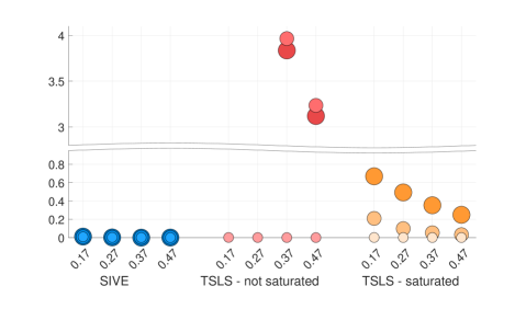
Figure 1: Average absolute bias in the estimand

Note: the figure shows the absolute median difference with the causal estimand in a setting without treatment heterogeneity. The size of the circles indicates the number of covariate groups with the small circle corresponding to $L=1$, the medium circle corresponding to $L=25$ and the large circle corresponding to $L=300$. The $x$-axis is the instrument strength $p(1)-p(0)$, with $p(0)=0.22$ and $p(1)=\{0.39,0.49,0.59,0.69\}$. Because non-saturated TSLS shows large biases for $L=25$ and $L=300$, the $y$-axis is broken between 0.9 and 3 and limited to $[0,4]$.

We see that SIVE is median unbiased regardless of the number of covariate groups and the values of $p(2)$ under consideration. For TSLS, we see that it is median unbiased for $L=1$ covariate group. However, as the number of covariate groups increases, non-saturated TSLS incurs a bias because estimand is non-causal. For saturated TSLS the (many instrument) bias enters. As is well known, this bias is more pronounced is settings where the instruments are weak. In the appendix we find that for JIVE1 removing the diagonal of the projection matrix leads to a large (omitted variable) bias as the controls are no longer correctly projected out. As we have shown in Section 2.4 this effect is mitigated by moving to the JIVE2 estimator. However, this estimator also shows an increasing bias with increasing number of covariate groups and an decreasing instrument strength.

Size

In Figure 2 we show that the size of a test of $H_{0}\colon\beta_{0}=\beta$ with $\beta=0.2$ in a setting without treatment heterogeneity (left panel) and with treatment heterogeneity (right panel). In the latter case, in (30) we set $\gamma_{i}=11$ for the 900 observations with the lowest values of $X_{i}$ and $\gamma_{i}=1$ for the remaining. The size of the circles indicates the number of covariate groups, which we choose as $L=\{1,25,100,300\}$. Given the large bias in non-saturated TSLS observed in Figure 1, we now only consider saturated TSLS. As expected TSLS yields accurate size control when $L=1$. For $L=25$, we have seen a substantial bias in Figure 1 and consequently we observe a size distortion that is increasing with decreasing instrument strength. For SIVE, we obtain close to nominal size control for $L=1$ for all values of the instrument strength. As expected based on the theory we see that for a larger number of covariate groups, the test becomes progressively more conservative. Increasing the instrument strength makes the test less conservative, as formalized in Corollary 1. The results with and without treatment heterogeneity do not show any qualitative differences.

Figure 2: Size versus instrument strength for an increasing number of instruments

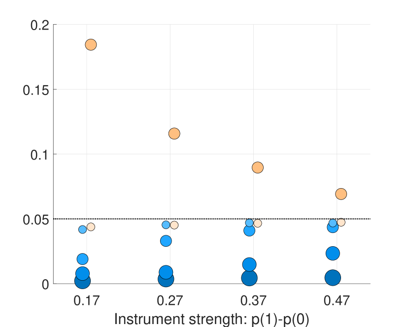
(a) Homogeneous treatment effects

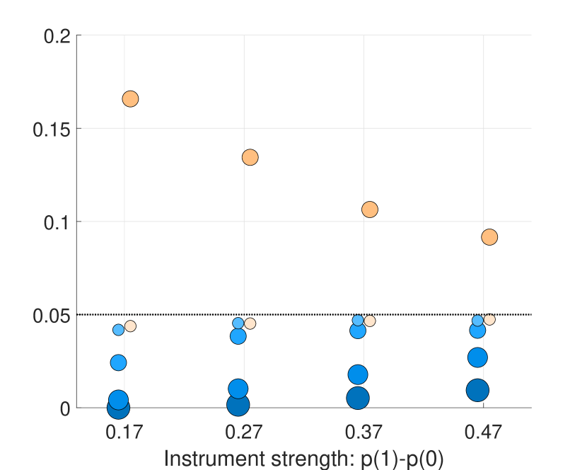
(b) Heterogeneous treatment effects

Note: the figure shows the size of testing $H_{0}\colon\beta=0.2$ at a nominal level of $5\%$. The $x$-axis is the instrument strength, with $p(0)=0.22$ and $p(1)=\{0.39,0.49,0.59,0.69\}$. The circles of increasing size correspond to $L=\{1,25,100,300\}$. TSLS is fully saturated and we use heteroskedasticity-robust (HC0) standard errors to construct the $t$-statistic. SIVE uses standard errors based on (20). The observed size for TSLS when $L=\{100,300\}$ is above 0.2.

Alternative variance estimators.

For SIVE, we use the variance estimator given in (20), which is robust to treatment effect heterogeneity. We first compare this with using the variance estimator proposed by Chao et al. (2023) that is given by

$$V_{c}=(T^{\prime}AD_{1}AT+(\hat{\varepsilon}\odot\hat{u})^{\prime}J(A\odot A)J(\hat{\varepsilon}\odot\hat{u}))/(T^{\prime}AT)^{2},$$ (31)

where $J=(M_{W}\odot M_{W})^{-1}$, $[D_{1}]_{i}=[J(\hat{\varepsilon}\odot\hat{\varepsilon})]_{i}$, $\hat{\varepsilon}=M_{W,Z}(y-T\hat{\beta}^{\text{SIVE}})=M_{W,Z}(\varepsilon-u\hat{\beta}^{\text{SIVE}})$ and $\hat{u}=M_{W,Z}T=M_{W,Z}u$. The variance estimator (31) is proposed in the context of a linear panel data model with homogeneous slope coefficient. We now assess the effect of treatment effect heterogeneity on tests that rely on (31).

In Figure 3 we show the size of the test of $H_{0}\colon\beta_{0}=\beta$ with $\beta=0.2$ in a setting with weak instruments ($p(2)=0.39$, left panel) and with strong instruments ($p(2)=0.69$, right panel). On the $x$-axis we vary the treatment effect heterogeneity through the parameter $\gamma_{i}=1+h$ with $h\in\{2,4,\ldots,10\}$ for the 900 observations with the smallest value of $X_{i}$ and $\gamma_{i}=1$ for the remaining. In the left panel, we again observe that SIVE offers a conservative test under weak instruments. As expected based on the theory, the level of heterogeneity has no effect on size of the test. For the alternative variance estimator, we see that increasing the level of treatment effect heterogeneity leads to a slightly oversized test, but no ordering in terms of the number of covariate groups is observed. The fact that treatment effect heterogeneity has only a mild effect in this case is due to the fact that the heterogeneity is flooded by the additional uncertainty introduced by the presence of many weak instruments. When the instruments are strong, as in the right panel of Figure 3, accounting for treatment effect heterogeneity becomes more important. Again, SIVE shows no dependence on the level of treatment effect heterogeneity. The alternative variance estimator now become progressively oversized as the level of heterogeneity increases for all values of the number of covariate groups.

Figure 3: Size versus treatment effect heterogeneity: compared to Chao et al. (2023).

(a) Weak identification

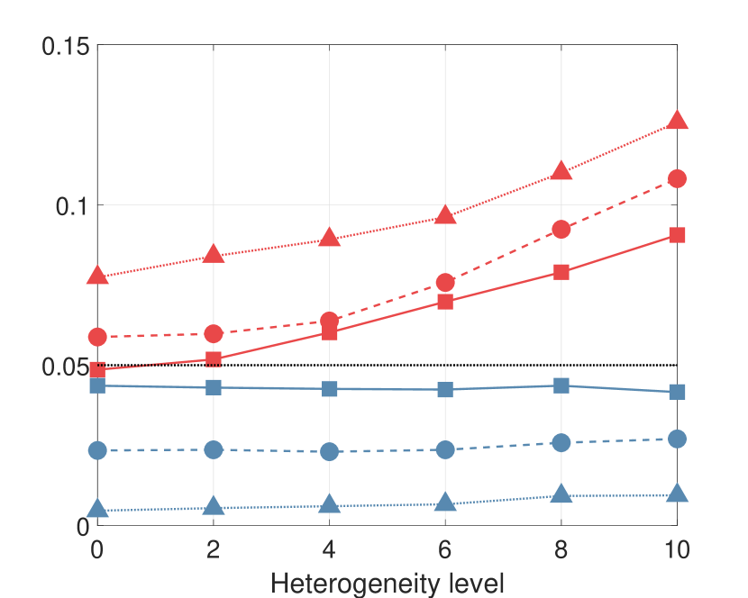
(b) Strong identification

Note: the figure shows the size of testing $H_{0}\colon\beta=\beta^{\text{SIVE}}$ at a nominal level of $5\%$. The left panel is for weak instruments, $p(2)-p(1)=0.17$, the right panel for strong instruments $p(2)-p(1)=0.47$. The $x$-axis is the heterogeneity level $h$. In (30), we set $\gamma_{i}=1+h$ with $h\in\{0,2,\ldots,10\}$ for the 900 observations with the smallest value of $X_{i}$ and $\gamma_{i}=1$ for the remaining. SIVC uses the SIVE estimator, but the variance estimator (31) proposed by Chao et al. (2023). We consider $L=\{25,100,300\}$ for the number of covariate groups, which correspond to the solid, dashed and dotted lines respectively.

Lee (2018) proposes a variance estimator for TSLS that is valid in overidentified systems where each instrument identifies a different LATE. It therefore allows for treatment effect heterogeneity. However, the analysis in Lee (2018) proceeds under the assumption that the number of instruments is fixed relative to the sample size. We therefore study its performance in a setting where the numbere of covariate groups $L$ increases.

In Figure 4, the left panel shows a setting with weak instruments $p(2)-p(1)=0.17$, the right panl a setting with strong instruments $p(2)-p(1)$. The variance estimator in Lee (2018) is designed for the right panel with a number of covariate groups that is small relative to the sample size. Indeed, for $L=\{2,25\}$ the variance estimator (dashed line, triangle markers) shows excellent size control and a substantial improvement over the standard Eicker-Huber-White variance estimator (solid line, circle markers). However, when the number of covariate groups increases, the many instrument bias manifests itself and the size increases above its nominal value. This effect is even stronger in the weakly identified setting in the left panel.

Figure 4: Size versus covariate groups: compared to Lee (2018).

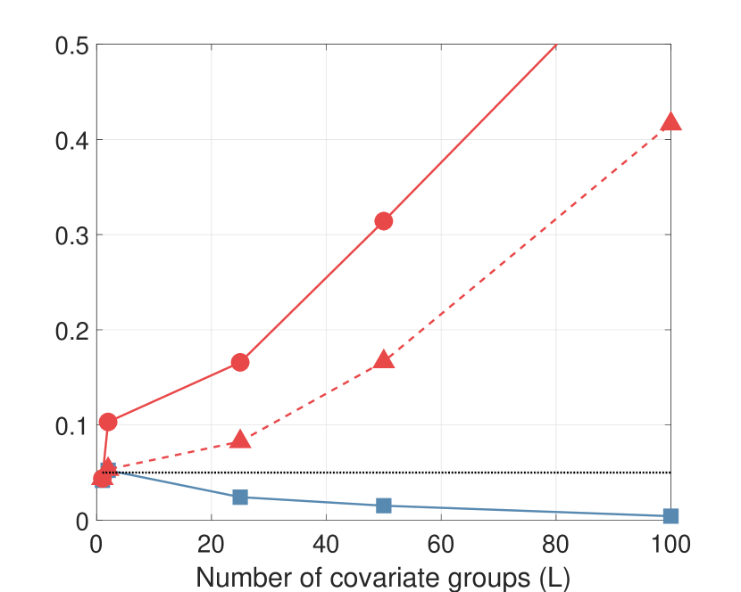
(a) Weak identification

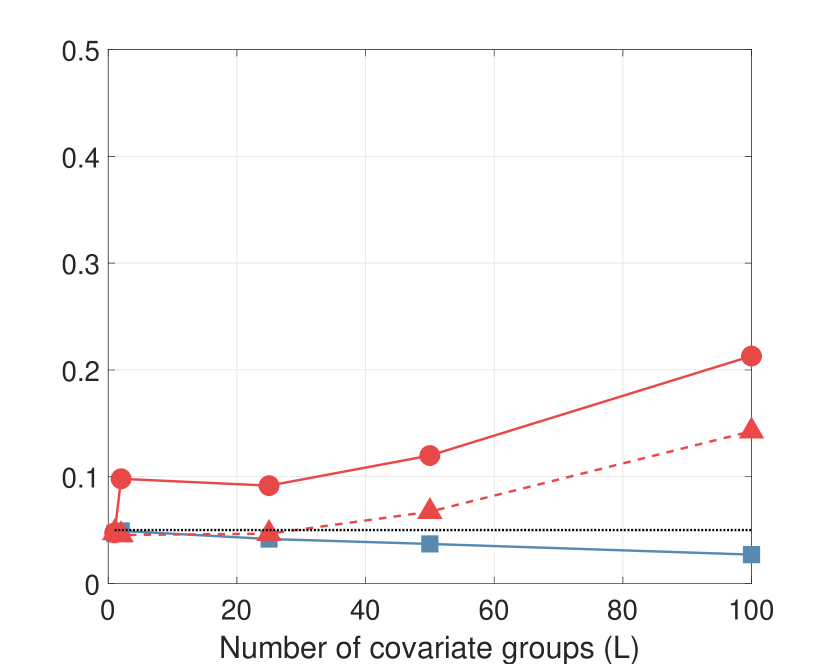
(b) Strong identification

Note: the figure shows the size of testing $H_{0}\colon\beta=\beta^{\text{SIVE}}$ at a nominal level of $5\%$. The $x$-axis is the number of covariate groups $L$. The left panel is for weak instruments, $p(2)-p(1)=0.17$, the right panel for strong instruments $p(2)-p(1)=0.47$. In (30), we set $\gamma_{i}=11$ for the 900 observations with the smallest value of $X_{i}$ and $\gamma_{i}=1$ for the remaining. The red solid line with circle marker is for TSLS, the red dashed line with triangle marker uses the variance estimator from Lee (2018), the blue solid line with square marker is for SIVE.

Application: Card (1995)

As an illustration of the proposed estimator and inference procedures we revisit the study by Card (1995) that uses the distance to the nearest college to instrument educational attainment. The data considers men aged 14-24 sampled in 1966 from the National Longitudinal Survey of Young Men (NLSYM). These men were followed until 1981. Following Card (1995), we consider individuals that provided education and wage information when they were interviewed in 1976.

Table 2: Empirical application: estimates, standard errors and confidence intervals

$(m_{g},n_{g}-m_{g})$	Estimator	Specification	Estimate	Standard error		95% CI
$\geq 2$	2SLS	not saturated	0.524	0.296	[	-0.056, 1.104	]
		fully saturated	0.156	0.138	[	-0.116, 0.427	]
		saturated instruments	0.209	0.102	[	0.009, 0.408	]
		saturated controls	0.570	0.298	[	-0.014, 1.154	]
	SIVE	fully saturated	0.125	0.342	[	-0.546, 0.795	]
		saturated instruments	0.217	0.171	[	-0.119 , 0.553	]
		saturated controls	0.644	0.440	[	-0.218 , 1.506	]
$\geq 3$	2SLS	not saturated	0.499	0.278	[	0.041, 0.957	]
		fully saturated	0.190	0.139	[	-0.038, 0.417	]
		saturated instruments	0.218	0.106	[	0.044, 0.392	]
		saturated controls	0.538	0.282	[	0.074, 1.001	]
	SIVE	fully saturated	0.215	0.273	[	-0.234, 0.664	]
		saturated instruments	0.233	0.159	[	-0.079 , 0.545	]
		saturated controls	0.599	0.388	[	-0.040 , 1.237	]

The instrument used by Card (1995) is the distance to the nearest four-year college. We consider some adjustments to the original model as proposed by Kitagawa (2015) and Słoczyński (2020). In particular, the specification includes five binary controls (Black, living in a metropolitan area (SMSA) in 1966, living in a metropolitan area (SMSA) in 1976, living in the South in 1966, living in the South in 1976). With these five binary controls, we potentially have 32 covariate groups after saturation. The original sample size is 3,010. We restrict the sample by requiring at least five observations in each covariate group, which brings the sample size to 2,988. In each of the covariate group we have at least two treated individuals and two non-treated individuals. Finally, we follow Kitagawa (2015) and Słoczyński (2020) and redefine the instrument to equal 1 if individuals have some college attendance (defined as having strictly more than 12 years of education) and 0 otherwise.

We consider the TSLS and SIVE estimators under different specifications for the controls and the instruments. First, the standard TSLS estimator that uses the binary instrument and linearly includes the controls. This estimator is inconsistent if the assumption of a linear relation with the controls is violated. Moreover, it supposes strong monotonicity in the instrument. We then saturate the model in the controls. To allow for weak monotonicity interact these controls with the instruments. This estimator is inconsistent due to the many instrument bias. We consider then two restricted versions of the fully saturated TSLS estimator. First, we only saturate in the controls, assuming strong monotonicity such that saturation in the instrument is not necessary. Second, we only saturate in the instrument, assuming a linear relation with the controls so that we do not need to saturate the controls. We follow the same specifications for SIVE with the exception of the model without any saturation.

Table 2 shows the point estimates, standard errors and 95% confidence intervals. For TSLS these are based on the HC0 based estimator for the variance covariance matrix. We reproduce the key findings by Słoczyński (2020). In particular, not interacting the instruments leads to unreasonably large estimates for the effect of schooling both when using TSLS and SIVE. When we saturate the instrument, the point estimates drop from around 0.5 to 0.2, which is much more in line with the recent literature on wage gains resulting from education. In terms of statistical efficiency, we see that the standard errors from SIVE are generally higher. This is to be expected as it takes into account the many instrument effect, as well as treatment effect heterogeneity.

If we have individuals that share the treatment status with only one other individual in the covariate group, we use the estimators from (22) that leads to an upward bias in the variance estimator (20). To analyze whether these individuals drive the results, we remove those individuals from the data. This reduces the sample size to 2,957 individuals. the bottom panel of Table 2 shows the point estimates, standard errors and confidence intervals of the methods. The main finding of interest is that the point estimate from the fully saturated SIVE slightly increases and is almost equal to that of the SIVE estimator that only saturates the instrument. Despite the smaller sample size, the standard errors are also somewhat lower.

Conclusion

We show how to conduct inference in a saturated IV model where the number of covariate values is of the same order as the sample size. The estimator is consistent under a minimal assumption on the identification strength. Crucially, and unlike existing procedures we allow arbitrary treatment effect heterogeneity. Our findings are confirmed through numerical experiments that rely on data with similar characteristics to the data analyzed by Card (1995). Applying the proposed estimator to that data yields realistic point estimates.

Appendix to “Inference on LATEs with covariates"

Appendix A Conventions and notation

Without loss of generality, we assume that the observations are ordered according to the columns of the matrix $W$ that contains the dummies indicating the values of the control variate(s) in the sense that

$$W=\left(\begin{array}[]{cccc}\iota_{n_{1}}&0_{n_{1}}&\ldots&0_{n_{1}}\\ 0_{n_{2}}&\iota_{n_{2}}&\ldots&0_{n_{2}}\\ \vdots&\vdots&\ddots&\vdots\\ 0_{n_{G}}&0_{n_{G}}&\ldots&\iota_{n_{G}}\end{array}\right).$$ (32)

As a subsequent ordering, we assume again without loss of generation that the matrix with instrument interactions has the following structure

$$Z=\left(\begin{array}[]{llll}\iota_{m_{1}}&0_{m_{1}}&\ldots&0_{m_{1}}\\ 0_{n_{1}-m_{1}}&0_{n_{1}-m_{1}}&\ldots&0_{n_{1}-m_{1}}\\ 0_{m_{2}}&\iota_{m_{2}}&\ldots&0_{m_{2}}\\ 0_{n_{2}-m_{2}}&0_{n_{2}-m_{2}}&\ldots&0_{n_{2}-m_{2}}\\ \vdots&\vdots&\ddots&\vdots\\ 0_{m_{G}}&0_{m_{G}}&\ldots&\iota_{m_{G}}\\ 0_{n_{G}-m_{G}}&0_{n_{G}-m_{G}}&\ldots&0_{n_{G}-m_{G}}\end{array}\right).$$ (33)

Throughout we denote by $r_{n}=G\mu_{n}$ under strong identification and $r_{n}=G$ under weak identification as defined in the main paper.

For any vector $v$, $v_{(g)}$ is the vector of observations from $v$ that have $W_{ig}=1$. Additionally, $v_{(g,1)}$ is the vector of observations that have $Z_{ig}=1$ and $v_{(g,2)}$ is the vector of observations that have $W_{ig}=1$ and $Z_{ig}=0$.

Appendix B Generalizations

This section extends the binary treatment and binary instrument setting to a multivalued treatment and instrument using respectively Theorem 1 and Theorem 2 in (Angrist and Imbens, 1995).

Multivalued treatment

Suppose the multivalued treatment $T_{i}$ takes values in the set $\{0,1,2,\dots,J\}$, where $T_{i}=0$ corresponds to no treatment, and $T_{i}=1,\dots,J$ correspond to different treatment levels. Define $D_{ij}=\mathbb{1}[T_{i}\geq j]$ with $D_{ij}=(1-Q_{i})D_{ij}(0)+Q_{i}D_{ij}(1)$. Under Assumption 1.2, we have

$$\begin{split}Y_{i}&=\sum_{j=0}^{J}(D_{i,j}-D_{i,j+1})Y_{i}(j)\\ &=(1-Q_{i})\sum_{j=0}^{J}(D_{i,j}(0)-D_{i,j+1}(0))Y_{i}(j)+Q_{i}\sum_{j=0}^{J}(D_{i,j}(1)-D_{i,j+1}(1))Y_{i}(j),\end{split}$$ (34)

where we use that $D_{i0}=1$ and $D_{i,J+1}=0$. It follows from Assumption 1.1 that

$$\begin{split}\theta(x_{g})&=\mathbb{E}[Y_{i}|Q_{i}=1,X_{i}={x}_{g}]-\mathbb{E}[Y_{i}|Q_{i}=0,X_{i}={x}_{g}]\\ &=\sum_{j=0}^{J}\mathbb{E}[(D_{i,j}(1)-D_{i,j+1}(1)-D_{i,j}(0)+D_{i,j+1}(0))Y_{i}(j)|X_{i}={x}_{g}]\\ &=\sum_{j=1}^{J}\mathbb{E}[(D_{i,j}(1)-D_{i,j}(0))(Y_{i}(j)-Y_{i}(j-1))|X_{i}={x}_{g}].\end{split}$$ (35)

From Assumption 1.4 follows that either $T_{i}(1)\geq T_{i}(0)$ or $T_{i}(1)\leq T_{i}(0)$ for all $i$ with $X_{i}=x_{g}$. Hence, we either have $D_{i,j}(1)=D_{i,j}(0)$, $D_{i,j}(1)>D_{i,j}(0)$, or $D_{i,j}(1)<D_{i,j}(0)$, where the latter two cases occur if $\max(T_{i}(1),T_{i}(0))\geq j>\min(T_{i}(1),T_{i}(0))$. It follows that

$$\theta(x_{g})= \sum_{j=1}^{J}\mathbb{E}[Y_{i}(j)-Y_{i}(j-1)|D_{i,j}(1)-D_{i,j}(0)\neq 0,X_{i}={x}_{g}]\mathbb{P}[D_{i,j}(1)-D_{i,j}(0)\neq 0|X_{i}={x}_{g}]$$ (36)

$$= \sum_{j=1}^{J}\mathbb{E}[Y_{i}(j)-Y_{i}(j-1)|\max(T_{i}(1),T_{i}(0))\geq j>\min(T_{i}(1),T_{i}(0)),X_{i}={x}_{g}]$$ (37)

$$\times\mathbb{P}[\max(T_{i}(1),T_{i}(0))\geq j>\min(T_{i}(1),T_{i}(0))|X_{i}={x}_{g}].$$ (38)

Similarly, we have

$$\begin{split}\pi(x_{g})&=\mathbb{E}[T_{i}|Q_{i}=1,X_{i}={x}_{g}]-\mathbb{E}[T_{i}|Q_{i}=0,X_{i}={x}_{g}]\\ &=\sum_{j=1}^{J}\mathbb{E}[D_{i,j}(1)-D_{i,j}(0)|X_{i}={x}_{g}]\\ &=\sum_{j=1}^{J}\mathbb{P}[D_{i,j}(1)-D_{i,j}(0)\neq 0|X_{i}={x}_{g}]\\ &=\sum_{j=1}^{J}\mathbb{P}[\max(T_{i}(1),T_{i}(0))\geq j>\min(T_{i}(1),T_{i}(0))|X_{i}={x}_{g}].\end{split}$$ (39)

Hence, with a multivalued treatment we obtain a covariate-specific weighted average of LATEs, known as an average causal response:

$$\tau(x_{g})=\frac{\theta(x_{g})}{\pi(x_{g})}= \sum_{j=1}^{J}\mathbb{E}\left[Y_{i}(j)-Y_{i}(j-1)|\max(T_{i}(1),T_{i}(0))\geq j>\min(T_{i}(1),T_{i}(0)),X_{i}={x}_{g}\right]$$ (40)

$$\times\frac{\mathbb{P}[\max(T_{i}(1),T_{i}(0))\geq j>\min(T_{i}(1),T_{i}(0))|X_{i}={x}_{g}]}{\sum_{j=1}^{J}\mathbb{P}[\max(T_{i}(1),T_{i}(0))\geq j>\min(T_{i}(1),T_{i}(0))|X_{i}=x_{g}]}$$ (41)

$$= \sum_{j=1}^{J}\eta_{j}\mathbb{E}\left[Y_{i}(j)-Y_{i}(j-1)|\max(T_{i}(1),T_{i}(0))\geq j>\min(T_{i}(1),T_{i}(0)),X_{i}={x}_{g}\right],$$ (42)

where

$$\eta_{j}=\frac{\mathbb{P}[\max(T_{i}(1),T_{i}(0))\geq j>\min(T_{i}(1),T_{i}(0))|X_{i}={x}_{g}]}{\sum_{j=1}^{J}\mathbb{P}[\max(T_{i}(1),T_{i}(0))\geq j>\min(T_{i}(1),T_{i}(0))|X_{i}=x_{g}]},$$ (43)

with $\sum_{j}\eta_{j}=1$. From Assumption 1.3 follows that $\mathbb{P}[\max(T_{i}(1),T_{i}(0))\geq j>\min(T_{i}(1),T_{i}(0))|X_{i}=x_{g}]>0$ for at least one treatment level $j$, and therefore $\eta_{j}\geq 0$ for all $j$. It follows that $\tau(x_{g})$ identifies an retains its causal interpretation with a multivalued treatment $T$. Note that with $J=1$ the result boils down to the covariate-specific LATE with a binary treatment.

Since all results in this paper are written in terms of $\tau(x_{g})$ using the reduced form and first stage (in which $T$ is written in terms of $Z$ and $W$), they directly apply to the multivalued treatment setting.

Multivalued instrument

Suppose we have $L$ mutually exclusive binary instruments $Q_{il}$ with $l=1,\dots,L$. This set of instruments may be interpreted as $L$ different instruments, which includes a full set of interactions across an original set of instruments in case they are not mutually exclusive, or the $L$ levels in a single instrument. The instruments in the set are ordered such that $l<k$ implies that $\mathbb{E}[T_{i}|Q_{il}=1,X_{i}=x_{g}]<\mathbb{E}[T_{i}|Q_{ik}=1,X_{i}=x_{g}]$. Define $Q_{i,0}=1-\sum_{l=1}^{L}Q_{il}$. The $LG\times 1$ vector $Z_{i}$ contains the instrument interactions $Z_{igl}=Q_{il}W_{ig}$, and $Z$ is defined as an $n\times LG$ matrix with $Z_{i}$ as rows.

Define

$$\tau_{l,l-1}(x_{g})=\frac{E[Y_{i}|Q_{il}=1,X_{i}={x}_{g}]-E[Y_{i}|Q_{i,l-1}=1,X_{i}={x}_{g}]}{E[T_{i}|Q_{il}=1,X_{i}={x}_{g}]-E[T_{i}|Q_{i,l-1}=1,X_{i}={x}_{g}]}.$$ (44)

It follows from Lemma 1 that $\tau_{l,l-1}(x_{g})=\mathbb{E}[Y_{i}(1)-Y_{i}(0)|T_{i}(l)\neq T_{i}(l-1),X_{i}=x_{g}]$ identifies a LATE.

We can write

$$\begin{split}&E[Y_{i}|Q_{il}=1,X_{i}={x}_{g}]\\ &=\tau_{l,l-1}(x_{g})\left(E[T_{i}|Q_{il}=1,X_{i}={x}_{g}]-E[T_{i}|Q_{i,l-1}=1,X_{i}={x}_{g}]\right)+E[Y_{i}|Q_{i,l-1}=1,X_{i}={x}_{g}]\\ &=\sum_{k=1}^{l}\tau_{k,k-1}(x_{g})\left(E[T_{i}|Q_{ik}=1,X_{i}={x}_{g}]-E[T_{i}|Q_{i,k-1}=1,X_{i}={x}_{g}]\right)+E[Y_{i}|Q_{i,0}=1,X_{i}={x}_{g}],\end{split}$$ (45)

and therefore

$$\theta_{l}(x_{g})= E[Y_{i}|Q_{il}=1,X_{i}={x}_{g}]-E[Y_{i}|Q_{i,0}=1,X_{i}={x}_{g}]$$ (46)

$$= \sum_{k=1}^{l}\tau_{k,k-1}(x_{g})\left(E[T_{i}|Q_{ik}=1,X_{i}={x}_{g}]-E[T_{i}|Q_{i,k-1}=1,X_{i}={x}_{g}]\right).$$ (47)

Similarly, we have

$$\pi_{l}(x_{g})= E[T_{i}|Q_{il}=1,X_{i}={x}_{g}]-E[T_{i}|Q_{i,0}=1,X_{i}={x}_{g}]$$ (48)

$$= \sum_{k=1}^{l}\left(E[T_{i}|Q_{ik}=1,X_{i}={x}_{g}]-E[T_{i}|Q_{i,k-1}=1,X_{i}={x}_{g}]\right).$$ (49)

Hence,

$$\tau_{l}(x_{g})=\frac{\theta_{l}(x_{g})}{\pi_{l}(x_{g})}=\sum_{k=1}^{l}\tau_{k,k-1}(x_{g})\frac{\left(E[T_{i}|Q_{ik}=1,X_{i}={x}_{g}]-E[T_{i}|Q_{i,k-1}=1,X_{i}={x}_{g}]\right)}{\sum_{k=1}^{l}\left(E[T_{i}|Q_{ik}=1,X_{i}={x}_{g}]-E[T_{i}|Q_{i,k-1}=1,X_{i}={x}_{g}]\right)},$$ (50)

which is a weighted average of LATEs with weights that sum up to one and are nonnegative due to the ordering of the instruments. Note that with $l=1$ the result boils down to the covariate-specific LATE with one instrument.

Instead of averaging over $G$ covariate-specific LATEs $\tau(x_{g})$, $\tau$ will be a weighted average of $LG$ covariate-specific weighted average of LATEs $\tau_{l}(x_{g})$ with multiple instruments. By substituting the following two expressions in the theoretical derivations in the paper, it follows that the weights are nonnegative and sum to one:

$$\pi^{\prime}Z^{\prime}M_{W}Z\theta= \sum_{g}\sum_{l}m_{gl}(1-\frac{m_{gl}}{n_{g}})\pi_{gl}(x_{g})\theta_{l}(x_{g}),$$ (51)

$$\pi^{\prime}Z^{\prime}M_{W}Z\pi= \sum_{g}\sum_{l}m_{gl}(1-\frac{m_{gl}}{n_{g}})\pi_{l}(x_{g})^{2},$$ (52)

where $\pi$ and $\theta$ are $LG\times 1$ vectors containing respectively $\pi_{gl}(x_{g})$ and $\theta_{l}(x_{g})$, and $m_{gl}=\sum_{i}Z_{igl}$.

Appendix C Proofs - Estimands

Proof Lemma 1

Using the exclusion restriction in Assumption 1.2, the observed outcomes are linked to the potential outcomes as $Y_{i}=(1-T_{i})Y_{i}(0)+T_{i}Y_{i}(1)=Y_{i}(0)+T_{i}\Delta_{i}$ with $\Delta_{i}=Y_{i}(1)-Y_{i}(0)$. The observed treatment is linked to the potential treatment statuses as $T_{i}=(1-Q_{i})T_{i}(0)+Q_{i}T_{i}(1)=T_{i}(0)+(T_{i}(1)-T_{i}(0))Q$. Hence, $Y_{i}=Y_{i}(0)+T_{i}(0)\Delta_{i}+(T_{i}(1)-T_{i}(0))\Delta_{i}Q_{i}$. We can now write

$$\begin{split}&\frac{E[Y_{i}|Q_{i}=1,X_{i}={x}_{g}]-E[Y_{i}|Q_{i}=0,X_{i}={x}_{g}]}{E[T_{i}|Q_{i}=1,X_{i}={x}_{g}]-E[T_{i}|Q_{i}=0,X_{i}={x}_{g}]}\\ &=\frac{E[Y_{i}(0)+T_{i}(0)\Delta_{i}+(T_{i}(1)-T_{i}(0))\Delta_{i}|Q_{i}=1,X_{i}={x}_{g}]-E[Y_{i}(0)+T_{i}(0)\Delta_{i}|Q_{i}=0,X_{i}={x}_{g}]}{E[T_{i}(1)|Q_{i}=1,X_{i}={x}_{g}]-E[T_{i}(0)|Q_{i}=0,X_{i}={x}_{g}]}\\ &=\frac{E[(T_{i}(1)-T_{i}(0))\Delta_{i}|X_{i}={x}_{g}]}{E[T_{i}(1)-T_{i}(0)|X_{i}={x}_{g}]}=\frac{E[\Delta_{i}|T_{i}(1)\neq T_{i}(0),X_{i}={x}_{g}]P[T_{i}(1)\neq T_{i}(0)=1|X_{i}={x}_{g}]}{P[T_{i}(1)\neq T_{i}(0)=1|X_{i}={x}_{g}]}\\ &=E[\Delta_{i}|T_{i}(1)\neq T_{i}(0),X_{i}={x}_{g}],\end{split}$$ (53)

using subsequently Assumption 1.1 independence and 1.4 monotonicity in the third line, and 1.3 relevance in the fourth line.

Proof Lemma 2

In a saturated specification, we can write

$$\begin{split}T_{i}&=\sum_{g}(\mathbb{E}[T_{i}|Z_{ig}=1,W_{ig}=1]-\mathbb{E}[T_{i}|Z_{ig}=0,W_{ig}=1])Z_{ig}+\mathbb{E}[T_{i}|Z_{ig}=0,W_{ig}=1]W_{ig}+u_{i},\\ Y_{i}&=\sum_{g}(\mathbb{E}[Y_{i}|Z_{ig}=1,W_{ig}=1]-\mathbb{E}[Y_{i}|Z_{ig}=0,W_{ig}=1])Z_{ig}+\mathbb{E}[Y_{i}|Z_{ig}=0,W_{ig}=1]W_{ig}+\varepsilon_{i},\end{split}$$ (54)

where $u_{i}=T_{i}-\mathbb{E}[T_{i}|Q_{i},X_{i}]$ and $\varepsilon_{i}=Y_{i}-\mathbb{E}[Y_{i}|Q_{i},X_{i}]$. It follows from the derivations in Section C.1 that this can be written as

$$T_{i} =\pi^{\prime}Z_{i}+\psi^{\prime}W_{i}+u_{i},$$ (55)

$$Y_{i} =\theta^{\prime}Z_{i}+\phi^{\prime}W_{i}+\varepsilon_{i},$$ (56)

where $\pi=(\pi(x_{1}),\dots,\pi(x_{g}))^{\prime}$ with $\pi(x_{g})=\mathbb{P}[T_{i}(1)\neq T_{i}(0)|X_{i}=x_{g}]$, $\psi=(\psi_{1},\dots,\psi_{g})^{\prime}$ with $\psi_{g}=\mathbb{E}[T_{i}|Z_{ig}=0,W_{ig}=1]$, $\theta=(\theta(x_{1}),\dots,\theta(x_{g}))^{\prime}$ with $\theta(x_{g})=\tau(x_{g})\mathbb{P}[T_{i}(1)\neq T_{i}(0)|X_{i}=x_{g}]$, and $\phi=(\phi_{1},\dots,\phi_{g})^{\prime}$ with $\phi_{g}=\mathbb{E}[Y_{i}|Z_{ig}=0,W_{ig}=1]$.

For the TSLS estimand, we now obtain the following.

$$\begin{split}\beta^{\text{TSLS}}=&\frac{\mathbb{E}[T^{\prime}PY|Q,X]}{\mathbb{E}[T^{\prime}PT|Q,X]}=\frac{\mathbb{E}[(Z\pi+u)^{\prime}P(Z\theta+\varepsilon)|Q,X]}{\mathbb{E}[(Z\pi+u)^{\prime}P(Z\pi+u)|Q,X]}\\ =&\frac{\pi^{\prime}Z^{\prime}PZ\theta+\pi^{\prime}Z^{\prime}P\mathbb{E}[\varepsilon|Q,X]+\mathbb{E}[u|Q,X]^{\prime}PZ\theta+\mathbb{E}[u^{\prime}P\varepsilon|Q,X]}{\pi^{\prime}Z^{\prime}PZ\pi+2\pi^{\prime}Z^{\prime}P\mathbb{E}[u|Q,X]+\mathbb{E}[u|Q,X]^{\prime}PZ\theta+\mathbb{E}[u^{\prime}Pu|Q,X]}\\ =&\frac{\pi^{\prime}Z^{\prime}M_{W}Z\theta+\mathbb{E}[u^{\prime}P\varepsilon|Q,X]}{\pi^{\prime}Z^{\prime}M_{W}Z\pi+\mathbb{E}[u^{\prime}Pu|Q,X]}\\ =&\frac{\sum_{g}\frac{\theta(x_{g})}{\pi(x_{g})}\pi(x_{g})^{2}n_{g}\frac{m_{g}}{n_{g}}(1-\frac{m_{g}}{n_{g}})+\sum_{i}\mathbb{E}[u_{i}\varepsilon_{i}|Q_{i},X_{i}]P_{ii}}{\sum_{g}\pi(x_{g})^{2}n_{g}\frac{m_{g}}{n_{g}}(1-\frac{m_{g}}{n_{g}})+\sum_{i}\mathbb{E}[u_{i}^{2}|Q_{i},X_{i}]P_{ii}}\\ =&\frac{\sum_{g}\frac{n_{g}}{n}\pi(x_{g})^{2}\frac{m_{g}}{n_{g}}(1-\frac{m_{g}}{n_{g}})\tau(x_{g})+\frac{1}{n}\sum_{i}\mathbb{E}[u_{i}\varepsilon_{i}|Q_{i},X_{i}]P_{ii}}{\sum_{g}\frac{n_{g}}{n}\pi(x_{g})^{2}\frac{m_{g}}{n_{g}}(1-\frac{m_{g}}{n_{g}})+\frac{1}{n}\sum_{i}\mathbb{E}[u_{i}^{2}|Q_{i},X_{i}]P_{ii}},\end{split}$$ (57)

where we use that $Z^{\prime}M_{W}Z$ is a $G\times G$ diagonal matrix with elements $n_{g}\frac{m_{g}}{n_{g}}(1-\frac{m_{g}}{n_{g}})$.

Note that $e_{i}^{\prime}M_{W}Z$ is a $1\times G$ vector with as elements the residual of observation $i$ in the regression of $Z_{ig}$ on $W_{ig}$, so $[e_{i}^{\prime}M_{W}Z]_{g}=Z_{ig}-W_{ig}\tilde{\text{P}}[Z_{i}=1|X_{i}=x_{g}]$, where $\tilde{\text{P}}[Z_{i}=1|X_{i}=x_{g}]=\frac{m_{g}}{n_{g}}$. Hence, $P_{ii}=e_{i}^{\prime}M_{W}Z(Z^{\prime}M_{W}Z)^{-1}Z^{\prime}M_{W}e_{i}=\sum_{g}\frac{1}{n_{g}}W_{ig}\frac{(Z_{ig}-\tilde{\text{P}}[Q_{i}=1|X_{i}=x_{g}])^{2}}{\text{Var}[Q_{i}|X_{i}=x_{g}]}$.

Proof Lemma 3

For the JIVE1 estimator we have

$$\begin{split}\beta^{\text{JIVE1}}=\frac{\mathbb{E}[T^{\prime}(P-D_{P})Y|Q,X]}{\mathbb{E}[T^{\prime}(P-D_{P})T|Q,X]}=\frac{\mathbb{E}[T^{\prime}PY|Q,X]-\mathbb{E}[T^{\prime}D_{P}Y|Q,X]}{\mathbb{E}[T^{\prime}PT|Q,X]-\mathbb{E}[T^{\prime}D_{P}T|Q,X]},\end{split}$$ (58)

with

$$\begin{split}\mathbb{E}[T^{\prime}D_{P}Y|Q,X]=&\mathbb{E}[(Z\pi+W\psi+u)^{\prime}D_{P}(Z\theta+W\phi+\varepsilon)|Q,X]\\ =&\pi^{\prime}Z^{\prime}D_{P}Z\theta+\pi^{\prime}Z^{\prime}D_{P}W\phi+\pi^{\prime}Z^{\prime}D_{P}\mathbb{E}[\varepsilon|Q,X]\\ &\quad+\psi^{\prime}W^{\prime}D_{P}Z\theta+\psi^{\prime}W^{\prime}D_{P}W\phi+\psi^{\prime}W^{\prime}D_{P}\mathbb{E}[\varepsilon|Q,X]\\ &\quad+\mathbb{E}[u|Q,X]^{\prime}D_{P}W\phi+\mathbb{E}[u|Q,X]^{\prime}D_{P}Z\theta+\mathbb{E}[u^{\prime}D_{P}\varepsilon|Q,X]\\ =&\pi^{\prime}Z^{\prime}D_{P}Z\theta+\pi^{\prime}Z^{\prime}D_{P}W\phi+\psi^{\prime}W^{\prime}D_{P}Z\theta+\psi^{\prime}W^{\prime}D_{P}W\phi+\mathbb{E}[u^{\prime}D_{P}\varepsilon|Q,X]\\ =&\sum_{g}(\frac{\theta(x_{g})}{\pi(x_{g})}\pi(x_{g})^{2}+\pi(x_{g})\phi_{g}+\theta(x_{g})\psi_{g})(1-\frac{m_{g}}{n_{g}})+\psi_{g}\phi_{g}+\sum_{i}\mathbb{E}[u_{i}\varepsilon_{i}|Q_{i},X_{i}]P_{ii},\end{split}$$ (59)

where $W^{\prime}D_{P}W=I_{G}$ as $\sum_{i}W_{ig}^{2}P_{ii}=1$, and $Z^{\prime}D_{P}Z=W^{\prime}D_{P}Z$ is a $G\times G$ diagonal matrix with elements $\sum_{i}Z_{ig}^{2}P_{ii}=(1-\frac{m_{g}}{n_{g}})$. Similarly, we get

$$\begin{split}\mathbb{E}[T^{\prime}D_{P}T|Q,X]=&\sum_{g}(\pi(x_{g})^{2}+2\pi(x_{g})\psi_{g})(1-\frac{m_{g}}{n_{g}})+\psi_{g}^{2}+\sum_{i}\mathbb{E}[u_{i}\varepsilon_{i}|Q_{i},X_{i}]P_{ii}.\end{split}$$ (60)

Hence, using the results in Section C.2, we have

$$\begin{split}\beta^{\text{JIVE1}}=&\frac{\sum_{g}\frac{n_{g}}{n}\pi(x_{g})^{2}\frac{m_{g}}{n_{g}}(1-\frac{m_{g}}{n_{g}})\tau(x_{g})(1-\frac{1}{m_{g}})-\sum_{g}\frac{n_{g}}{n}(\pi(x_{g})\phi_{g}+\theta(x_{g})\psi_{g})\frac{m_{g}}{n_{g}}(1-\frac{m_{g}}{n_{g}})\frac{1}{m_{g}}-\frac{1}{n}\psi_{g}\phi_{g}}{\sum_{g}\frac{n_{g}}{n}\pi(x_{g})^{2}\frac{m_{g}}{n_{g}}(1-\frac{m_{g}}{n_{g}})(1-\frac{1}{m_{g}})-2\sum_{g}\frac{n_{g}}{n}\pi(x_{g})\psi_{g}\frac{m_{g}}{n_{g}}(1-\frac{m_{g}}{n_{g}})\frac{1}{m_{g}}-\frac{1}{n}\psi_{g}^{2}}\\ =&\frac{\sum_{g}\mathbb{P}[X_{i}=x_{g}]\pi(x_{g})^{2}\text{Var}[Q_{i}|X_{i}=x_{g}](1-\mathbb{P}[Q_{i}=1,X_{i}=x_{g}])\tau(x_{g})-B_{Y}}{\sum_{g}\mathbb{P}[X_{i}=x_{g}]\pi(x_{g})^{2}\text{Var}[Q_{i}|X_{i}=x_{g}](1-\mathbb{P}[Q_{i}=1,X_{i}=x_{g}])-B_{T}}\end{split}$$ (61)

where

$$\begin{split}B_{Y}=&\sum_{g}\mathbb{P}[X_{i}=x_{g}](\pi(x_{g})\phi_{g}+\theta(x_{g})\psi_{g})\text{Var}[Q_{i}|X_{i}=x_{g}]\mathbb{P}[Q_{i}=1,X_{i}=x_{g}]-\frac{1}{n}\psi_{g}\phi_{g},\\ B_{T}=&2\sum_{g}\mathbb{P}[X_{i}=x_{g}]\pi(x_{g})\psi_{g}\text{Var}[Q_{i}|X_{i}=x_{g}]\mathbb{P}[Q_{i}=1,X_{i}=x_{g}]-\frac{1}{n}\psi_{g}^{2},\end{split}$$ (62)

with $\tilde{\text{P}}[Q_{i}=1,X_{i}=x_{g}]=\frac{1}{m_{g}}$, $\psi_{g}=\mathbb{E}[T_{i}|Z_{ig}=0,W_{ig}=1]$, and $\phi_{g}=\mathbb{E}[Y_{i}|Z_{ig}=0,W_{ig}=1]$.

Proof Lemma 5

First we show that $P_{ii}=[M_{W,Z}DM_{W,Z}]_{ii}$ if the elements of the diagonal matrix $D$ are set equal to $D_{ii}=\sum_{k=1}^{n}[(M_{W,Z}\odot M_{W,Z})^{-1}]_{ik}P_{kk}$. Using that $D$ is diagonal and $M_{W,Z}$ symmetric, we have

$$\begin{split}[M_{W,Z}DM_{W,Z}]_{ii}&=\sum_{j}[M_{W,Z}\odot M_{W,Z}]_{ij}D_{jj}\\ &=\sum_{j}[M_{W,Z}\odot M_{W,Z}]_{ij}\sum_{k=1}^{n}P_{kk}[(M_{W,Z}\odot M_{W,Z})^{-1}]_{kj}\\ &=\sum_{k=1}^{n}P_{kk}\sum_{j}[M_{W,Z}\odot M_{W,Z}]_{ij}[(M_{W,Z}\odot M_{W,Z})^{-1}]_{kj}\\ &=P_{ii}.\end{split}$$ (63)

Next, we derive an expression for $D_{ii}$. Note that ${M}_{W,Z}$ is a block diagonal matrix with the $g$th block an $n_{g}\times n_{g}$ matrix

$$\begin{split}M_{W,Z,(g)}&=I_{n_{g}}-P_{W,Z,(g)}=I_{n_{g}}-\left(\begin{array}[]{cc}m_{g}^{-1}\iota_{m_{g}}\iota_{m_{g}}^{\prime}&O_{m_{g},n_{g}-m_{g}}\\ O_{n_{g}-m_{g},m_{g}}&(n_{g}-m_{g})^{-1}\iota_{n_{g}-m_{g}}\iota_{n_{g}-m_{g}}^{\prime}\end{array}\right),\end{split}$$ (64)

where the observations are ordered according to covariate group and within covariate group on active instrument, without loss of generality. It now follows that

$$\begin{split}[M_{W,Z}\odot M_{W,Z}]_{(g)}=\left(\begin{array}[]{cc}\left(1-\frac{2}{m_{g}}\right)I_{m_{g}}+\frac{1}{m_{g}^{2}}\iota_{m_{g}}\iota_{m_{g}}^{\prime}&O_{m_{g},n_{g}-m_{g}}\\ O_{n_{g}-m_{g},m_{g}}&\left(1-\frac{2}{n_{g}-m_{g}}\right)I_{n_{g}-m_{g}}+\frac{1}{(n_{g}-m_{g}))^{2}}\iota_{n_{g}-m_{g}}\iota_{n_{g}-m_{g}}^{\prime}\end{array}\right),\end{split}$$ (65)

and hence

$$\begin{split}[(M_{W,Z}\odot M_{W,Z})^{-1}]_{(g)}=\left(\begin{array}[]{cc}\frac{m_{g}}{m_{g}-2}\left(I_{m_{g}}-\frac{1}{m_{g}(m_{g}-1)}\iota_{m_{g}}\iota_{m_{g}}^{\prime}\right)&O_{m_{g},n_{g}-m_{g}}\\ O_{n_{g}-m_{g},m_{g}}&\frac{n_{g}-m_{g}}{n_{g}-m_{g}-2}\left(I_{n_{g}-m_{g}}-\frac{1}{(n_{g}-m_{g})(n_{g}-m_{g}-1)}\iota_{n_{g}-m_{g}}\iota_{n_{g}-m_{g}}^{\prime}\right)\end{array}\right).\end{split}$$ (66)

Note that $P_{ii}=\sum_{g}\frac{1}{n_{g}}W_{ig}\frac{(Z_{ig}-\frac{m_{g}}{n_{g}})^{2}}{\frac{m_{g}}{n_{g}}(1-\frac{m_{g}}{n_{g}})}$, as derived in Section C.2, and hence $P_{ii}=\frac{1}{m_{g}}-\frac{1}{n_{g}}$ if $W_{ig}=Z_{ig}=1$ and $P_{ii}=\frac{m_{g}/n_{g}}{n_{g}-m_{g}}$ if $W_{ig}=1$ and $Z_{ig}=0$. Define $[D_{P}]_{(g)}$ as the elements in the diagonal of $P$ corresponding to the observations in $[M_{W,Z}\odot M_{W,Z})^{-1}]_{(g)}$:

$$\begin{split}D_{ii}=&\sum_{g}W_{ig}e_{i}^{\prime}[(M_{W,Z}\odot M_{W,Z})^{-1}]_{(g)}[D_{P}]_{(g)}\\ =&\sum_{g}W_{ig}\left[\frac{m_{g}}{m_{g}-2}\left(1-\frac{m_{g}}{m_{g}(m_{g}-1)}\right)\left(\frac{1}{m_{g}}-\frac{1}{n_{g}}\right)Z_{ig}\right.\\ &\quad\left.+\frac{n_{g}-m_{g}}{n_{g}-m_{g}-2}(1-\frac{n_{g}-m_{g}}{(n_{g}-m_{g})(n_{g}-m_{g}-1)})\frac{m_{g}}{n_{g}(n_{g}-m_{g})}(1-Z_{ig})\right]\\ =&\sum_{g}\frac{1}{n_{g}}W_{ig}\left[\frac{n_{g}-m_{g}}{m_{g}-1}Z_{ig}+\frac{m_{g}}{n_{g}-m_{g}-1}(1-Z_{ig})\right].\end{split}$$ (67)

The derivation above implicitly assumes that $m_{g}\geq 3$ and $n_{g}-m_{g}\geq 3$ for all expressions to be well-defined. However, the end result only requires $m_{g}\geq 2$ and $n_{g}-m_{g}\geq 2$. We can briefly verify whether $D_{ii}$ as given on the final line of (67) indeed yields a zero diagonal for $P-M_{W,Z}DM_{W,Z}.$

Consider observation $i$ for which $Z_{ig}=1$. Then,

$$\begin{split}P_{ii}&=\frac{1}{n_{g}}\frac{n_{g}-m_{g}}{m_{g}},\quad D_{ii}=\frac{1}{n_{g}}\frac{n_{g}-m_{g}}{m_{g}-1},\quad P_{W,Z,ii}=\frac{1}{m_{g}}.\end{split}$$ (68)

Since $D_{ii}$ is the same for all observations that have $Z_{ig}=1$, we have

$$[M_{W,Z}DM_{W,Z}]_{ii}=D_{ii}(1-2P_{W,Z,ii})+m_{g}\frac{1}{m_{g}^{2}}D_{ii}=D_{ii}(1-P_{W,Z,ii})=D_{ii}\frac{m_{g}-1}{m_{g}}=P_{ii}.$$ (69)

The case where $Z_{ig}=0$ follows analogously.

Proof Theorem 1

$$\begin{split}\beta^{\text{SIVE}}=\frac{\mathbb{E}[T^{\prime}(P-M_{W,Z}DM_{W,Z})Y|Q,X]}{\mathbb{E}[T^{\prime}(P-M_{W,Z}DM_{W,Z})T|Q,X]}=\frac{\mathbb{E}[T^{\prime}PY|Q,X]-\mathbb{E}[T^{\prime}M_{W,Z}DM_{W,Z}Y|Q,X]}{\mathbb{E}[T^{\prime}PT|Q,X]-\mathbb{E}[T^{\prime}M_{W,Z}DM_{W,Z}T|Q,X]},\end{split}$$ (70)

with

$$\begin{split}\mathbb{E}[T^{\prime}M_{W,Z}DM_{W,Z}Y|Q,X]=&\mathbb{E}[u^{\prime}M_{W,Z}DM_{W,Z}\varepsilon|Q,X]=\sum_{i}\mathbb{E}[u_{i}\varepsilon_{i}|Q_{i},X_{i}]P_{ii},\end{split}$$ (71)

and similarly we have $\mathbb{E}[T^{\prime}M_{W,Z}DM_{W,Z}Y|Q,X]=\sum_{i}\mathbb{E}[u_{i}^{2}|Q_{i},X_{i}]P_{ii}$. Combining this result with the result in Section C.2, we have

$$\begin{split}\beta^{\text{SIVE}}=&\frac{\sum_{g}\frac{n_{g}}{n}\pi(x_{g})^{2}\frac{m_{g}}{n_{g}}(1-\frac{m_{g}}{n_{g}})\tau(x_{g})}{\sum_{g}\frac{n_{g}}{n}\pi(x_{g})^{2}\frac{m_{g}}{n_{g}}(1-\frac{m_{g}}{n_{g}})}.\end{split}$$ (72)

Appendix D Proofs - Inference

Preliminary results

D.1.1 The elements of the projection matrix $P$

Since the columns in $W$ are orthogonal, $P_{W}=W(W^{\prime}W)^{-1}W$ is a block diagonal matrix consisting of $G$ blocks of dimension $n_{g}\times n_{g}$. The $g$th block is given by $P_{(g)}=\frac{1}{n_{g}}\iota_{n_{g}}\iota_{n_{g}}^{\prime}$. We then have that

$$M_{W}Z=\left(\begin{array}[]{ccc}M_{\iota_{n_{1}}}z_{(1)}&0_{n_{1}}&\ldots\\ 0_{n_{2}}&M_{\iota_{n_{2}}}z_{(2)}&\ldots\\ \vdots&\vdots&\ddots\end{array}\right).$$ (73)

The matrix $P$ is again block diagonal, with

$$P=\left(\begin{array}[]{ccc}(z_{(1)}^{\prime}M_{\iota_{n_{1}}}z_{(1)})^{-1}M_{\iota_{n_{1}}}z_{(1)}z_{(1)}^{\prime}M_{\iota_{n_{1}}}&O_{n_{1},n_{2}}&\ldots\\ O_{n_{2},n_{1}}&(z_{(2)}^{\prime}M_{\iota_{n_{2}}}z_{(2)})^{-1}M_{\iota_{n_{2}}}z_{(2)}z_{(2)}^{\prime}M_{\iota_{n_{2}}}&\ldots\\ \vdots&\vdots&\ddots\end{array}\right).$$ (74)

The elements of $P$ are given by

$$\begin{split}[P]_{ij}&=\left\{\begin{array}[]{rl}\frac{1}{n_{g}}\frac{1-m_{g}/n_{g}}{m_{g}/n_{g}}&W_{ig}=W_{jg}=1,Z_{ig}=1,Z_{jg}=1,\\ -1/n_{g}&W_{ig}=W_{jg}=1,Z_{ig}=1,Z_{jg}=0,\\ -1/n_{g}&W_{ig}=W_{jg}=1,Z_{ig}=0,Z_{jg}=1,\\ \frac{1}{n_{g}}\frac{m_{g}/n_{g}}{1-m_{g}/n_{g}}&W_{ig}=W_{jg}=1,Z_{ig}=0,Z_{jg}=0,\\ 0&\text{otherwise.}\end{array}\right.\\ \end{split}$$ (75)

D.1.2 Results on the matrix $A$ used for asymptotic normality

Recall that $A=P-M_{W,Z}DM_{W,Z}$. This matrix is block diagonal with blocks

$$\begin{split}{A}_{(g)}&=\left(\begin{array}[]{cc}\frac{n_{g}-m_{g}}{n_{g}(m_{g}-1)}(\iota_{m_{g}}\iota_{m_{g}}^{\prime}-I_{m_{g}})&-\frac{1}{n_{g}}\iota_{m_{g}}\iota_{n_{g}-m_{g}}^{\prime}\\ -\frac{1}{n_{g}}\iota_{n_{g}-m_{g}}\iota_{m_{g}}^{\prime}&\frac{m_{g}}{n_{g}(n_{g}-m_{g}-1)}(\iota_{n_{g}-m_{g}}\iota_{n_{g}-m_{g}}^{\prime}-I_{n_{g}-m_{g}})\end{array}\right).\end{split}$$ (76)

The following result is used in the proof of the central limit theorem for the SIVE estimator,

$$\begin{split}\text{tr}(A^{2})&=G+\text{tr}(M_{W,Z}DM_{W,Z}D)\\ &=G+\sum_{i=1}^{n}D_{ii}^{2}-2\sum_{i=1}^{n}D_{ii}^{2}[P_{W,Z}]_{ii}+\text{tr}({P}_{W,Z}D{P}_{W,Z}D)\\ &=G+\sum_{g=1}^{G}m_{g}\frac{1}{n_{g}^{2}}\frac{(n_{g}-m_{g})^{2}}{(m_{g}-1)^{2}}+(n_{g}-m_{g})\frac{1}{n_{g}^{2}}\frac{m_{g}^{2}}{(n_{g}-m_{g}-1)^{2}}\\ &\quad-\sum_{g=1}^{G}\frac{1}{n_{g}^{2}}\frac{(n_{g}-m_{g})^{2}}{(m_{g}-1)^{2}}+\frac{1}{n_{g}^{2}}\frac{m_{g}^{2}}{(n_{g}-m_{g}-1)^{2}}\\ &=G+\sum_{g=1}^{G}\frac{1}{n_{g}^{2}}\left[\frac{(n_{g}-m_{g})^{2}}{m_{g}-1}+\frac{m_{g}^{2}}{n_{g}-m_{g}-1}\right]\\ &\leq G+\sum_{g=1}^{G}\left[\frac{1}{m_{g}-1}+\frac{1}{n_{g}-m_{g}-1}\right]\\ &\leq 3G,\end{split}$$ (77)

where the last line uses that $m_{g}\geq 2$ and $n_{g}-m_{g}\geq 2$. From the first line we also immediately have that

$$\text{tr}(A^{2})\geq G.$$ (78)

The eigenvalues of $A$ are $0$ with multiplicity 1, $1$ with multiplicity $1$, $-(n_{g}-m_{g})/(n_{g}(m_{g}-1))$ with multiplicity $m_{g}-1$ and $-m_{g}/(n_{g}(n_{g}-m_{g}-1))$ with multiplicity $n_{g}-m_{g}-1$. Since $m_{g}\geq 2$ and $n_{g}-m_{g}\geq 2$, we conclude that the eigenvalues are on the [-1,1] interval.

In the SIVE estimator, we encounter the product $AZ\pi$ and $AZ\zeta$. We require an elementwise bound on these products, which can be established as follows.

$$\begin{split}|[AZ\pi]_{i}|&=|[M_{W}Z\pi]_{i}|\\ &=\pi(x_{g})\left\{\begin{array}[]{ll}\frac{n_{g}-m_{g}}{n_{g}}&\text{if }Z_{ig}=1,W_{ig}=1,\\ \frac{m_{g}}{n_{g}}&\text{if }Z_{ig}=0,W_{ig}=1,\\ 0&\text{otherwise}.\end{array}\right.\\ &\leq C<\infty,\quad a.s.\end{split}$$ (79)

The same result follows for $AZ\zeta=AZ(\theta-\beta^{\text{SIVE}}\pi)$ by noting that $\theta(x_{g})/\pi(x_{g})=\tau(x_{g})\leq C<\infty$ $a.s.$ by Assumption 3.1.

D.1.3 Results on the matrix $A$ used for consistency of the variance estimator

To show consistency of the variance estimator, we need to upper bound terms that are of the form

$$S(A,\bar{P})=\sum_{i_{1},\ldots,i_{16}}|A_{i_{1}i_{2}}||A_{i_{3}i_{4}}||A_{i_{5}i_{6}}||A_{i_{7}i_{8}}|\bar{P}_{i_{9}i_{10}}\bar{P}_{i_{11}i_{12}}\bar{P}_{i_{13}i_{14}}\bar{P}_{i_{15}i_{16}},$$ (80)

with some restrictions on the indices over which we sum. We will first find a matrix $\tilde{A}$ such that $S(A,\bar{P})\leq S(\tilde{A},\bar{P})$. To save on notation, define

$$\begin{split}H_{g}&=\left(\begin{array}[]{cc}\iota_{m_{g}}&0_{m_{g}}\\ 0_{n_{g}-m_{g}}&\iota_{n_{g}-m_{g}}\end{array}\right),\quad E_{g}=\left(\begin{array}[]{cc}m_{g}^{-1}&0\\ 0&(n_{g}-m_{g})^{-1}\end{array}\right)\end{split}$$ (81)

We then have

$$\begin{split}{A}_{(g)}&=\left(\begin{array}[]{cc}\frac{n_{g}-m_{g}}{n_{g}(m_{g}-1)}(\iota_{m_{g}}\iota_{m_{g}}^{\prime}-I_{m_{g}})&-\frac{1}{n_{g}}\iota_{m_{g}}\iota_{n_{g}-m_{g}}^{\prime}\\ -\frac{1}{n_{g}}\iota_{n_{g}-m_{g}}\iota_{m_{g}}^{\prime}&\frac{m_{g}}{n_{g}(n_{g}-m_{g}-1)}(\iota_{n_{g}-m_{g}}\iota_{n_{g}-m_{g}}^{\prime}-I_{n_{g}-m_{g}})\end{array}\right)\\ &=\frac{m_{g}(n_{g}-m_{g})}{n_{g}}\left(\begin{array}[]{cc}\frac{1}{m_{g}(m_{g}-1)}(\iota_{m_{g}}\iota_{m_{g}}^{\prime}-I_{m_{g}})&-\frac{1}{m_{g}(n_{g}-m_{g})}\iota_{m_{g}}\iota_{n_{g}-m_{g}}^{\prime}\\ -\frac{1}{m_{g}(n_{g}-m_{g})}\iota_{n_{g}-m_{g}}\iota_{m_{g}}^{\prime}&\frac{1}{(n_{g}-m_{g})(n_{g}-m_{g}-1)}(\iota_{n_{g}-m_{g}}\iota_{n_{g}-m_{g}}^{\prime}-I_{n_{g}-m_{g}})\end{array}\right)\\ &\leq 2\frac{m_{g}(n_{g}-m_{g})}{n_{g}}H_{g}E_{g}\iota_{2}\iota_{2}^{\prime}E_{g}H_{g}^{\prime}\equiv\tilde{A}_{(g)},\end{split}$$ (82)

where $\leq$ indicates an elementwise inequality.

We can now establish the following results

$$\begin{array}[]{crl}(R1)&\text{tr}(\tilde{A}_{(g)})&\leq C,\\ (R2)&\lambda_{\max}(\tilde{A}_{(g)})&\leq C,\\ (R3)&\tilde{A}_{(g)}^{2}&=2\tilde{A}_{(g)},\\ (R4)&\tilde{A}_{(g)}{P}_{W,Z,(g)}&=\tilde{A}_{(g)},\\ (R5)&\iota_{n_{g}}^{\prime}(\tilde{A}_{(g)}\odot{P}_{W,Z,(g)})\iota_{n_{g}}&\leq C,\\ (R6)&\iota_{n_{g}}^{\prime}(\tilde{A}_{(g)}\odot{P}_{W,Z,(g)})^{2}\iota_{n_{g}}&\leq C,\\ (R7)&\iota_{n_{g}}^{\prime}(\tilde{A}_{(g)}\odot{P}_{W,Z,(g)})\tilde{A}_{(g)}\iota_{n_{g}}&\leq C,\\ (R8)&\iota_{n_{g}}^{\prime}\tilde{A}_{(g)}({P}_{W,Z,(g)}\odot{P}_{W,Z,(g)})\tilde{A}_{(g)}\iota_{n_{g}}&\leq C.\end{array}$$ (83)

Proof: (R1) follows from the fact that $H_{g}^{\prime}H_{g}=E_{g}^{-1}$, $\iota_{n_{g}}^{\prime}H_{g}=\iota_{2}^{\prime}E_{g}^{-1}$ and $\iota_{2}^{\prime}E_{g}\iota_{2}=\frac{n_{g}}{m_{g}(n_{g}-m_{g})}$. Since $\text{rank}(\tilde{A}_{(g)})=1$, (R2) follows from (R1). (R3) follows from the fact that $H_{g}^{\prime}H_{g}=E_{g}^{-1}$. For $(R4)--(R8)$, we first note that the $g$th diagonal block of the projection matrix $P_{W,Z}$ satisfies ${P}_{W,Z,(g)}=H_{g}E_{g}H_{g}^{\prime}$. Using this result and again the fact that $H_{g}^{\prime}H_{g}=E_{g}^{-1}$ yields (R4). For (R5), we note that $\iota_{n_{g}}^{\prime}(\tilde{A}_{(g)}\odot{P}_{W,Z,(g)})\iota_{n_{g}}=\text{tr}(\tilde{A}_{(g)}{P}_{W,Z,(g)})=\text{tr}(\tilde{A}_{(g)})$ with the last equality by (R4). For (R6) and (R7) we first calculate the elementwise product,

$$\begin{split}\tilde{A}_{(g)}\odot{P}_{W,Z,(g)}&=2\frac{m_{g}(n_{g}-m_{g})}{n_{g}}H_{g}E_{g}^{3}H_{g}^{\prime}.\end{split}$$ (84)

We can now explicitly calculate bounds for (R6) and (R7),

$$\begin{split}\iota_{n_{g}}^{\prime}(\tilde{A}_{(g)}\odot{P}_{W,Z,(g)})^{2}\iota_{n_{g}}&=4\frac{m_{g}^{2}(n_{g}-m_{g})^{2}}{n_{g}^{2}}(m_{g}^{-3}+(n_{g}-m_{g})^{-3})\\ &=4\frac{n_{g}^{3}-3n_{g}m_{g}^{2}-3n_{g}^{2}m_{g}}{n_{g}^{3}(n_{g}-m_{g})}\leq 4\frac{1}{n_{g}}\leq 2,\\ \iota_{n_{g}}^{\prime}(\tilde{A}_{(g)}\odot{P}_{W,Z,(g)})\tilde{A}_{(g)}\iota_{n_{g}}&=4\frac{m_{g}^{2}(n_{g}-m_{g})^{2}}{n_{g}^{2}}(m_{g}^{-2}+(n_{g}-m_{g})^{-2})\leq 8,\end{split}$$ (85)

For (R8), we have a similar result as,

$$\begin{split}\iota_{n_{g}}^{\prime}\tilde{A}_{(g)}({P}_{W,Z,(g)}\odot{P}_{W,Z,(g)})\tilde{A}_{(g)}\iota_{n_{g}}&=4\frac{m_{g}^{2}(n_{g}-m_{g})^{2}}{n_{g}^{2}}(m_{g}^{-2}+(n_{g}-m_{g})^{-2})\leq 8.\end{split}$$ (86)

Finally, we establish the following results.

$$\begin{array}[]{crl}(R9)&\iota_{n_{g}}^{\prime}(\tilde{A}_{(g)}\odot\tilde{A}_{(g)})^{2}\iota_{n_{g}}&=16\frac{m_{g}^{2}(n_{g}-m_{g})^{2}}{n_{g}^{2}}\iota_{2}^{\prime}E_{g}^{3}\iota_{2}\leq 16,\\ (R10)&\iota_{n_{g}}^{\prime}\tilde{A}_{(g)}(\tilde{A}_{g}\odot\tilde{A}_{(g)})\tilde{A}_{(g)}\iota_{n_{g}}&\leq 256,\\ (R11)&(\iota_{n_{g}}^{\prime}(\tilde{A}_{(g)}\odot\tilde{A}_{(g)})((\tilde{A}_{(g)}\iota_{n_{g}})\odot(\tilde{A}_{(g)}\iota_{n_{g}}))&\leq 128.\end{array}$$ (87)

From the definition of $\tilde{A}_{(g)}$, we have

$$\tilde{A}_{(g)}\odot\tilde{A}_{(g)} =4\frac{m_{g}^{2}(n_{g}-m_{g})^{2}}{n_{g}^{2}}H_{g}E_{g}^{2}\iota_{2}\iota_{2}^{\prime}E_{g}^{2}H_{g}^{\prime},$$ (88)

$$\tilde{A}_{(g)}\iota_{n_{g}} =4\frac{m_{g}(n_{g}-m_{g})}{n_{g}}H_{g}E_{g}\iota_{2},$$ (89)

$$(\tilde{A}_{(g)}\iota_{n_{g}})\odot(\tilde{A}_{(g)}\iota_{n_{g}}) =16\frac{m_{g}^{2}(n_{g}-m_{g})^{2}}{n_{g}^{2}}H_{g}E_{g}^{2}\iota_{2},$$ (90)

$$(\tilde{A}_{(g)}\odot\tilde{A}_{(g)})\iota_{n_{g}} =4\frac{m_{g}(n_{g}-m_{g})}{n_{g}}H_{g}E_{g}^{2}\iota_{2}.$$ (91)

The first equality in $(R9)$ then follows from (91) and using that $H_{g}^{\prime}H_{g}=E_{g}^{-1}$. Then $(R9)$ follows from the following.

$$\begin{split}\frac{m_{g}^{2}(n_{g}-m_{g})^{2}}{n_{g}^{2}}\iota_{2}^{\prime}E_{g}^{3}\iota_{2}&=\frac{m_{g}^{2}(n_{g}-m_{g})^{2}}{n_{g}^{2}}\frac{m_{g}^{3}+(n_{g}-m_{g})^{3}}{m_{g}^{3}(n_{g}-m_{g})^{3}}\\ &=\frac{n_{g}^{3}-3n_{g}^{2}m_{g}-3n_{g}m_{g}^{2}}{n_{g}^{2}m_{g}(n_{g}-m_{g})}\\ &\leq\frac{n_{g}^{3}-3n_{g}^{2}m_{g}-3n_{g}m_{g}^{2}}{n_{g}^{3}}\leq 1,\end{split}$$ (92)

where the first inequality uses that $m_{g}(n_{g}-m_{g})\geq 2(n_{g}-2)\geq 2(n_{g}-n_{g}/2)=n_{g}$ since $n_{g}\geq 4$ by Assumption 2.

For $(R10)$, using first (88) and then (89),

$$\begin{split}\iota_{n_{g}}^{\prime}\tilde{A}_{(g)}(\tilde{A}_{(g)}\odot\tilde{A}_{(g)})\tilde{A}_{(g)}\iota_{n_{g}}&=64\frac{m_{g}^{4}(n_{g}-m_{g})^{4}}{n_{g}^{4}}(\iota_{2}^{\prime}E_{g}^{2}\iota_{2})^{2}=64\frac{(m_{g}^{2}+(n_{g}-m_{g})^{2})^{2}}{n_{g}^{4}}\leq 256.\end{split}$$ (93)

Finally, for $(R11)$ using (90) and (91), we have

$$\begin{split}(\iota_{n_{g}}^{\prime}(\tilde{A}_{(g)}\odot\tilde{A}_{(g)})((\tilde{A}_{(g)}\iota_{n_{g}})\odot(\tilde{A}_{(g)}\iota_{n_{g}}))&=64\frac{m_{g}^{3}(n_{g}-m_{g})^{3}}{n_{g}^{3}}\iota_{2}^{\prime}E_{g}^{3}\iota_{2}=64\frac{m_{g}^{3}+(n_{g}-m_{g})^{3}}{n_{g}^{3}}\leq 128.\end{split}$$ (94)

D.1.4 First stage and reduced form error (co)variance estimators

From the reduced form equation (56) and first stage (55), we see that $M_{W,Z}T=M_{W,Z}u$ and $M_{W,Z}(Y-T\beta^{\text{SIVE}})=M_{W,Z}v$. We now have the following estimators,

$$\begin{split}\hat{\sigma}_{u,i}^{2}&=e_{i}^{\prime}(M_{W,Z}\odot M_{W,Z})^{-1}(M_{W,Z}T\odot M_{W,Z}T)\\ &=e_{i}^{\prime}(M_{W,Z}\odot M_{W,Z})^{-1}(M_{W,Z}u\odot M_{W,Z}u)\\ \hat{\sigma}_{uv,i}&=e_{i}^{\prime}(M_{W,Z}\odot M_{W,Z})^{-1}(M_{W,Z}(Y-T\hat{\beta}^{\text{SIVE}})\odot M_{W,Z}T)\\ &=e_{i}^{\prime}(M_{W,Z}\odot M_{W,Z})^{-1}(M_{W,Z}(Y-T\beta^{\text{SIVE}})\odot M_{W,Z}T)-(\hat{\beta}^{\text{SIVE}}-\beta^{\text{SIVE}})\hat{\sigma}_{u,i}^{2}\\ &=e_{i}^{\prime}(M_{W,Z}\odot M_{W,Z})^{-1}(M_{W,Z}v\odot M_{W,Z}u)-(\hat{\beta}^{\text{SIVE}}-\beta^{\text{SIVE}})\hat{\sigma}_{u,i}^{2}\\ &=\hat{\sigma}_{uv,i}(\beta^{\text{SIVE}})-(\hat{\beta}^{\text{SIVE}}-\beta^{\text{SIVE}})\hat{\sigma}_{u,i}^{2},\\ \hat{\sigma}_{v,i}^{2}&=e_{i}^{\prime}(M_{W,Z}\odot M_{W,Z})^{-1}(M_{W,Z}(Y-T\hat{\beta}^{\text{SIVE}})\odot M_{W,Z}(Y-T\hat{\beta}^{\text{SIVE}}))\\ &=e_{i}^{\prime}(M_{W,Z}\odot M_{W,Z})^{-1}(M_{W,Z}(Y-T{\beta^{\text{SIVE}}})\odot M_{W,Z}(Y-T{\beta^{\text{SIVE}}}))\\ &\quad-2(\hat{\beta}^{\text{SIVE}}-\beta^{\text{SIVE}})\hat{\sigma}_{uv,i}(\beta^{\text{SIVE}})+(\hat{\beta}^{\text{SIVE}}-\beta^{\text{SIVE}})^{2}\hat{\sigma}_{u,i}^{2}\\ &=e_{i}^{\prime}(M_{W,Z}\odot M_{W,Z})^{-1}(M_{W,Z}v\odot M_{W,Z}v)\\ &\quad-2(\hat{\beta}^{\text{SIVE}}-\beta^{\text{SIVE}})\hat{\sigma}_{uv,i}(\beta^{\text{SIVE}})+(\hat{\beta}^{\text{SIVE}}-\beta^{\text{SIVE}})^{2}\hat{\sigma}_{u,i}^{2}\\ &=\hat{\sigma}_{v,i}^{2}(\beta^{\text{SIVE}})-2(\hat{\beta}^{\text{SIVE}}-\beta^{\text{SIVE}})\hat{\sigma}_{uv,i}(\beta^{\text{SIVE}})+(\hat{\beta}^{\text{SIVE}}-\beta^{\text{SIVE}})^{2}\hat{\sigma}_{u,i}^{2},\end{split}$$ (95)

where we write $\hat{\sigma}_{v,i}^{2}(\beta^{\text{SIVE}})$ and $\hat{\sigma}_{uv,i}(\hat{\beta}^{\text{SIVE}}$ as the infeasible analogues of $\hat{\sigma}_{uv,i}$ and $\hat{\sigma}_{v,i}^{2}$ with $\hat{\beta}^{\text{SIVE}}$ replaced by $\beta^{\text{SIVE}}$. Since $\hat{\beta}^{\text{SIVE}}-\beta^{\text{SIVE}}=o_{p}(1)$, we will see that the contribution of the corresponding terms in $\hat{\sigma}_{uv,i}$ and $\hat{\sigma}_{v,i}^{2}$ to the variance estimator for the score is $o_{p}(1)$ as well.

We first show that $\hat{\sigma}_{u,i}^{2}$, $\hat{\sigma}_{uv,i}(\beta^{\text{SIVE}})$ and $\hat{\sigma}_{v,i}^{2}(\beta^{\text{SIVE}})$ are unbiased for $\sigma_{u,i}^{2}$, $\sigma_{uv,i}$ and $\sigma_{v,i}^{2}$, respectively. To save on space, we denote the elements of $P_{W,Z}$ as $\bar{P}_{ij}$. From the properties of $M_{W,Z}$ and using that $\bar{P}_{ij}=m_{g}^{-1}$ if $Z_{ig}=Z_{jg}=1$, $\bar{P}_{ij}=(n_{g}-m_{g})^{-1}$ if $Z_{ig}=Z_{jg}=0$, and $W_{ig}=W_{jg}=1$ and ${P}_{ij}=0$ elsewhere, we can write

$$\begin{split}\hat{\sigma}_{u,i}^{2}&=u_{i}^{2}-u_{i}\frac{2}{1-2\bar{P}_{ii}}\sum_{j\neq i}\bar{P}_{ij}u_{j}+\frac{1}{(1-\bar{P}_{ii})(1-2\bar{P}_{ii})}\sum_{j=1}^{n}\sum_{k\neq j}\bar{P}_{ij}\bar{P}_{ik}u_{j}u_{k},\\ \hat{\sigma}_{v,i}^{2}(\beta^{\text{SIVE}})&=v_{i}^{2}-v_{i}\frac{2}{1-2\bar{P}_{ii}}\sum_{j\neq i}\bar{P}_{ij}v_{j}+\frac{1}{(1-\bar{P}_{ii})(1-2\bar{P}_{ii})}\sum_{j=1}^{n}\sum_{k\neq j}\bar{P}_{ij}\bar{P}_{ik}v_{j}v_{k},\\ \hat{\sigma}_{uv,i}(\beta^{\text{SIVE}})&=u_{i}v_{i}-v_{i}\frac{1}{1-2\bar{P}_{ii}}\sum_{j\neq i}\bar{P}_{ij}u_{j}-u_{i}\frac{1}{1-2\bar{P}_{ii}}\sum_{j\neq i}\bar{P}_{ij}v_{j}+\frac{1}{(1-\bar{P}_{ii})(1-2\bar{P}_{ii})}\sum_{j=1}^{n}\sum_{k\neq j}\bar{P}_{ij}\bar{P}_{ik}u_{j}v_{k}.\end{split}$$ (96)

Taking the conditional expectation and using independence across $i$, we see that $\hat{\sigma}_{u,i}^{2}$, $\hat{\sigma}_{uv,i}(\beta^{\text{SIVE}})$ and $\hat{\sigma}_{v,i}^{2}(\beta^{\text{SIVE}})$ are (conditionally) unbiased for $\sigma_{u,i}^{2}$, $\sigma_{uv,i}$ and $\sigma_{v,i}^{2}$, respectively. What is important to note is that the estimators only exist if $m_{g}>2$ and $n_{g}-m_{g}>2$ for all $g=1,\ldots,G$. We discuss how we handle groups with $m_{g}=2$ or $n_{g}-m_{g}=2$ in Section D.3.3.

Proof Lemma 6

Let $\hat{\beta}^{\text{SIVE}}-\beta^{\text{SIVE}}=S_{n}/D_{n}$ with

$$\begin{split}S_{n}&=r_{n}^{-1/2}T^{\prime}A(Y-T\beta^{\text{SIVE}}),\\ D_{n}&=r_{n}^{-1/2}T^{\prime}AT.\end{split}$$ (97)

We refer to $S_{n}$ as the score vector. Let $\zeta=\theta-\beta^{\text{SIVE}}\pi$ and $v_{i}=\varepsilon_{i}-u_{i}\beta^{\text{SIVE}}$ with $\varepsilon_{i}$ and $u_{i}$ defined in the reduced form equations (55) and (56). Denote $\sigma_{u,i}^{2}=\mathbb{E}[u_{i}^{2}|Q,X]$, $\sigma_{v,i}^{2}=\mathbb{E}[v_{i}^{2}|Q,X]$, and $\sigma_{uv,i}=\mathbb{E}[u_{i}v_{i}|Q,X]$.

We have $\mathbb{E}[S_{n}|Q,X]=0$ and

$$\begin{split}\mathbb{V}(S_{n}|Q,X)&=r_{n}^{-1}\sum_{i=1}^{n}\sigma_{u,i}^{2}[M_{W}Z\zeta]_{i}^{2}+\sigma_{v,i}^{2}[M_{W}Z\pi]_{i}^{2}+2\sigma_{uv,i}[M_{W}Z\pi]_{i}[M_{W}Z\zeta]_{i}\\ &\qquad+r_{n}^{-1}\sum_{i=1}^{n}\sum_{j\neq i}A_{ij}^{2}(\sigma_{uv,i}\sigma_{uv,j}+\sigma_{v,i}^{2}\sigma_{u,i}^{2})\\ &\leq C[r_{n}^{-1}\zeta^{\prime}Z^{\prime}M_{W}Z\zeta+r_{n}^{-1}\pi^{\prime}Z^{\prime}M_{W}Z\pi)+r_{n}^{-1}\text{tr}(A^{2})]\leq C,\quad a.s.,\end{split}$$ (98)

where the first inequality follows from Assumption 3.3 and the second inequality from Assumption 3.1, the definition of $r_{n}$ and (77). For $D_{n}$, we have $\mathbb{E}[D_{n}|Q,X]=r_{n}^{-1/2}\pi^{\prime}Z^{\prime}M_{W}Z\pi\equiv r_{n}^{1/2}H_{n}$ and

$$\begin{split}\mathbb{V}(D_{n}|Q,X)&\leq 4r_{n}^{-1}\mathbb{E}[(u^{\prime}M_{W}Z\pi)^{2}|Q,X]+r_{n}^{-1}\mathbb{E}[(u^{\prime}Au)^{2}|Q,X]\\ &\leq 4\max_{i}\sigma_{u,i}^{2}r_{n}^{-1}\pi^{\prime}Z^{\prime}M_{W}Z\pi+2r_{n}^{-1}\max_{i}\sigma_{u,i}^{4}\text{tr}(A^{2})\leq C,\quad a.s.\end{split}$$ (99)

We can now write

$$\begin{split}\hat{\beta}^{\text{SIVE}}-\beta^{\text{SIVE}}&=\frac{r_{n}^{-1/2}T^{\prime}A(Y-T\beta^{\text{SIVE}})/(r_{n}^{1/2}H_{n})}{1+r_{n}^{1/2}(r_{n}^{-1}T^{\prime}AT-H_{n})/(r_{n}^{1/2}H_{n})}=\frac{A_{n}}{B_{n}}.\end{split}$$ (100)

Assume that $r_{n}^{-1/2}H_{n}^{-1}\rightarrow_{p}0$. From (98) it follows that $A_{n}\rightarrow_{p}0$. From (99) we have that $r_{n}^{1/2}(r_{n}^{-1}T^{\prime}AT-H_{n})/(r_{n}^{1/2}H_{n})\rightarrow_{p}0$, and hence $B_{n}\rightarrow_{p}1$. We conclude that when $(r_{n}^{1/2}H_{n})^{-1}=\big{(}r_{n}^{-1/2}\pi^{\prime}Z^{\prime}M_{W}Z\pi\big{)}^{-1}\rightarrow_{p}0$, the SIVE estimator is consistent: $\hat{\beta}^{\text{SIVE}}-\beta^{\text{SIVE}}\rightarrow_{p}0$. Finally, we have under weak identification, $r_{n}^{1/2}H_{n}=\sqrt{G}\frac{\pi^{\prime}Z^{\prime}M_{W}Z\pi}{G}=\sqrt{G}\frac{n\text{FS}}{G}=\sqrt{G}\mu_{n}$ so that requiring that $r_{n}^{-1/2}H_{n}^{-1}\rightarrow_{p}0$ is the same as the requirement in Lemma 6 that $\sqrt{G}\mu_{n}\rightarrow_{p}\infty$. This completes the proof.

Proof Theorem 2

The proof of Theorem 2 is long, so we start with a brief overview of the steps. First, we establish asymptotic normality of the score vector $S_{n}$ defined in (97) after normalizing it with the square root of its conditional variance. This step relies on a central limit theorem for quadratic forms of growing rank. We then show that the difference between the estimator for the conditional variance given in (20) and the population conditional variance converges in probability to a quantity larger than zero (under weak identification) or equal to zero (under strong identification). This step uses the properties of the regression error variance estimators (21). The derivation is somewhat tedious as it requires to keep track of higher-order interactions of the first stage and reduced form regression errors. Finally, we analyze the use of the variance estimator (22) when we encounter covariate groups with $m_{g}=2$ or $n_{g}-m_{g}=2$.

D.3.1 Asymptotic normality of the self-normalized score

As in the previous subsection, we rewrite

$$\begin{split}r_{n}^{1/2}(\hat{\beta}^{\text{SIVE}}-\beta^{\text{SIVE}})&=\frac{r_{n}^{-1/2}T^{\prime}A(Y-T\beta^{\text{SIVE}})}{r_{n}^{-1}T^{\prime}AT}=\frac{S_{n}}{r_{n}^{-1/2}D_{n}}.\end{split}$$ (101)

The variance of $S_{n}$ is given in the first line of (98). We now study the self-normalized version of $S_{n}$ given by

$$S_{n}^{*}=\frac{r_{n}^{-1/2}T^{\prime}A(Y-T\beta)}{\mathbb{V}(S_{n}|Q,X)^{1/2}}.$$ (102)

To show that $S_{n}^{*}\rightarrow_{d}N(0,1)$, we use Lemma D.2 in Evdokimov and Kolesár (2018), which in turn is based on Lemma A.2 in Chao et al. (2012).

Lemma 7

[Evdokimov and Kolesár (2018), Lemma D.2] Define $R=t^{\prime}u+s^{\prime}v+u^{\prime}\bar{A}v$, where $[\bar{A}]_{ii}=0$. Suppose that the following holds almost surely.

1. $\mathbb{E}[u_{i}|Q,X]=\mathbb{E}[v_{i}|Q,X]=0$ and $\mathbb{E}[u_{i}^{4}|Q,X]\leq C<\infty$ and $\mathbb{E}[v_{i}^{4}|Q,X]\leq C<\infty$,

2. $\mathbb{V}(R|Q,X)^{-1}\leq C<\infty$,

3. $\sum_{i=1}^{n}(t_{i}^{4}+s_{i}^{4})\rightarrow 0$,

4. $\emph{tr}(\bar{A}^{4})\rightarrow 0$.

Then, $\mathbb{V}(R|Q,X)^{-1/2}R\rightarrow_{d}N(0,1).$

Let $R=S_{n}$, so that $t=r_{n}^{-1/2}M_{W}Z\zeta$ and $s=r_{n}^{-1/2}M_{W}Z\pi$ and $\bar{A}=r_{n}^{-1/2}A$. Moreover, $u_{i}$ is as defined in (55) and $v_{i}=\varepsilon_{i}-u_{i}\beta^{\text{SIVE}}$ with $\varepsilon_{i}$ as in (56).

Verifying Conditions 1–4. Condition 1: holds by Assumption 3. Condition 3: From (79) we see that $|e_{i}^{\prime}M_{W}Z\pi|\leq C<\infty$ $a.s.$ uniformly over $i$. Similarly, $|e_{i}^{\prime}M_{W}Z\zeta|\leq C<\infty$ $a.s.$ uniformly over $i$. We then obtain

$$\sum_{i=1}^{n}(t_{i}^{4}+s_{i}^{4})\leq Cr_{n}^{-2}\sum_{i=1}^{n}(t_{i}^{2}+s_{i}^{2})=Cr_{n}^{-1}(\pi^{\prime}Z^{\prime}M_{W}Z\pi/r_{n}+\zeta^{\prime}Z^{\prime}M_{W}Z\zeta/r_{n}).$$ (103)

The term in brackets is almost surely bounded as shown in Section D.2. Since $r_{n}^{-1}\rightarrow_{a.s.}0$, Condition (3) of Lemma 7 holds. To verify Condition 2 and Condition 4 we separately consider strong and weak/vanishing identification.

Strong identification

We start by showing that in Lemma 7 we have $u^{\prime}\bar{A}v=o_{p}(1)$ so that we only have to verify Condition 2. We first note that

$$\begin{split}\mathbb{V}(G^{-1/2}u^{\prime}Av|Q,X)&=G^{-1}\sum_{j\neq i}\sum_{k\neq m}A_{ij}A_{mk}\mathbb{E}[u_{i}u_{k}v_{j}v_{m}|Q,X]\\ &=G^{-1}\sum_{j\neq i}A_{ij}^{2}(\mathbb{E}[u_{i}v_{i}u_{j}v_{j}|Q,X]+\mathbb{E}[u_{i}^{2}v_{j}^{2}|Q,X])\\ &\leq CG^{-1}\text{tr}(A^{2})\leq C\quad a.s.,\end{split}$$ (104)

using that $u_{i}$ and $v_{i}$ have bounded fourth conditional moment by Assumption 3 and the bound established in (77). Then, by the definition of $r_{n}$ in the case of strong identification,

$$\mathbb{V}(u^{\prime}Av|Q,X)/r_{n}\leq CG/r_{n}\rightarrow_{a.s.}0.$$ (105)

We can then conclude that $r_{n}^{-1/2}u^{\prime}Av=o_{p}(1)$. Therefore, it suffices to consider $\tilde{R}=t^{\prime}u+s^{\prime}v$ and we only need to verify Condition 2. As in (98),

$$\begin{split}\mathbb{V}(\tilde{R}|Q,X)&=r_{n}^{-1}\sum_{i=1}^{n}\sigma_{u,i}^{2}[M_{W}Z\zeta]_{i}^{2}+\sigma_{v,i}^{2}[M_{W}Z\pi]_{i}^{2}+2\sigma_{uv,i}[M_{W}Z\pi]_{i}[M_{W}Z\zeta]_{i}.\end{split}$$ (106)

Denote $g(i)$ a function such that $g(i)=g$ if $w_{ig}=1$. By Assumption 3, using (79),

$$\begin{split}\mathbb{V}(\tilde{R}|Q,X)&=r_{n}^{-1}\sum_{i=1}^{n}c_{i}^{2}\bigg{(}\zeta(x_{g(i)})^{2}\sigma_{u,i}^{2}+\pi(x_{g(i)})^{2}\sigma_{v,i}^{2}+2\pi(x_{g(i)})\zeta(x_{g(i)})\sigma_{uv,i}\bigg{)}\\ &=r_{n}^{-1}\sum_{i=1}^{n}c_{i}^{2}[\zeta(x_{g(i)}),\pi(x_{g(i)})]\left(\begin{array}[]{cc}1&0\\ -\beta&1\end{array}\right)\Sigma_{i}\left(\begin{array}[]{cc}1&-\beta\\ 0&1\end{array}\right)[\zeta(x_{g(i)}),\pi(x_{g(i)})]^{\prime}\\ &\geq Cr_{n}^{-1}\sum_{i=1}^{n}c_{i}^{2}\left(\zeta(x_{g(i)})^{2}+\pi(x_{g(i)})^{2}\right),\end{split}$$ (107)

where $\Sigma_{i}=\left(\begin{array}[]{cc}\sigma_{u,i}^{2}&\sigma_{u\varepsilon,i}\\ \sigma_{u\varepsilon,i}&\sigma_{\varepsilon_{i}}^{2}\end{array}\right)$ and $c_{i}=\sum_{g}Z_{ig}\frac{n_{g}-m_{g}}{n_{g}}-(W_{ig}-Z_{ig})\frac{m_{g}}{n_{g}}$. We have

$$\begin{split}r_{n}^{-1}\sum_{i=1}^{n}c_{i}^{2}\pi(x_{g(i)})^{2}&=r_{n}^{-1}\sum_{g=1}^{G}\pi(x_{g})^{2}\left[m_{g}\left(\frac{n_{g}-m_{g}}{n_{g}}\right)^{2}+(n_{g}-m_{g})\left(\frac{m_{g}}{n_{g}}\right)^{2}\right]\\ &=r_{n}^{-1}\sum_{g=1}^{G}\pi(x_{g})^{2}n_{g}\frac{m_{g}(n_{g}-m_{g})}{n_{g}^{2}}\\ &=1,\end{split}$$ (108)

where the last line uses the definition of $r_{n}$. We conclude that $\mathbb{V}(\tilde{R}|Q,X)\geq C>0$ $a.s.$ and Condition 2 of Lemma 7 holds.

Weak identification

We start with verifying Condition 2 in Lemma 7. By Assumption 3, $\min_{i=1,\ldots,n}\sigma_{v,i}^{2}\geq C>0$ and $\min_{i=1,\ldots,n}\sigma_{u,i}^{2}\geq C>0$. Then, using (78)

$$\begin{split}\mathbb{V}(S_{n}|Q,X)&\geq G^{-1}\text{tr}(D_{\sigma_{v}^{2}}AD_{\sigma_{u}^{2}}A)\\ &\geq CG^{-1}\text{tr}(A^{2})\\ &\geq C>0\quad a.s.\end{split}$$ (109)

For Condition 4, we have that $G^{-1}\text{tr}(A^{2})\leq 3$ $a.s.$ by (77) and $\lambda_{\max}(A^{2})=1$ since $\lambda_{\max}(A)=1$. Then,

$$\begin{split}\text{tr}(\bar{A}_{n}^{4})=r_{n}^{-2}\text{tr}(A^{4})&\leq\frac{G^{2}}{r_{n}^{2}}\frac{\text{tr}(A^{2})}{G}\frac{\lambda_{\max}(A^{2})}{G}\rightarrow_{a.s.}0.\end{split}$$ (110)

We note that these results are shown without any assumptions on the identification strength, so that we can base identification-robust inference on the asymptotic normality of the score vector.

We have now established asymptotic normality of the renormalized score vector under both weak and strong identification. To prove Theorem 2 the next step is to show that the numerator of the variance estimator in (20) converges to $\mathbb{V}(S_{n}|Q,X)$.

D.3.2 Consistency of the estimator for the variance of the score

We momentarily assume that $m_{g}\geq 3$ and $n_{g}-m_{g}\geq 3$ so that we can use (21) for the regression error variances and covariances. We relax this assumption in Section D.3.3.

We can rewrite the variance given in (98) as

$$\begin{split}\mathbb{V}(S_{n}|Q,X)&=r_{n}^{-1}\bigg{[}\zeta^{\prime}Z^{\prime}M_{W}D_{\sigma_{u}^{2}}M_{W}Z\zeta+\pi^{\prime}Z^{\prime}M_{W}D_{\sigma_{v}^{2}}M_{W}Z\pi+2\zeta^{\prime}Z^{\prime}M_{W}D_{\sigma_{uv}}M_{W}Z\pi\\ &\quad\quad+\underbrace{\iota^{\prime}D_{\sigma_{uv}}(A\odot A)D_{\sigma_{uv}}\iota+\iota^{\prime}D_{\sigma_{v}^{2}}(A\odot A)D_{\sigma_{u}^{2}}\iota}_{({B}.0)}\bigg{]}.\end{split}$$ (111)

In (20) we use the following estimator for $\mathbb{V}(S_{n}|Q,X)$.

$$\begin{split}\hat{\mathbb{V}}(S|Q,X)&=r_{n}^{-1}\left[(Y-T\hat{\beta}^{\text{SIVE}})^{\prime}AD_{\hat{\sigma}_{u}^{2}}A(Y-T\hat{\beta}^{\text{SIVE}})+T^{\prime}AD_{\hat{\sigma}_{v}^{2}}AT+2(Y-T\hat{\beta}^{\text{SIVE}})^{\prime}AD_{\hat{\sigma}_{uv}}AT\right].\end{split}$$ (112)

Let $D_{u^{2}}$ be a diagonal matrix with $[D_{u^{2}}]_{ii}=u_{i}^{2}$ and likewise for $D_{v^{2}}$ and $D_{uv}$. Consider the infeasible variance estimator

$$\begin{split}\mathbb{V}_{\inf}(S_{n}|Q,X)&=r_{n}^{-1}\bigg{[}\zeta^{\prime}Z^{\prime}M_{W}D_{u^{2}}M_{W}Z\zeta+\pi^{\prime}Z^{\prime}M_{W}D_{{v}^{2}}M_{W}Z\pi+2\zeta^{\prime}Z^{\prime}M_{W}D_{{uv}}M_{W}Z\pi\\ &\quad\quad+\iota^{\prime}D_{{uv}}(A\odot A)D_{{uv}}\iota+\iota^{\prime}D_{{v}^{2}}(A\odot A)D_{{u}^{2}}\iota\bigg{]}.\end{split}$$ (113)

We decompose (112) as

$$\begin{split}\hat{\mathbb{V}}(S|Q,X)&=r_{n}^{-1}\left[(Z\zeta+v-T(\hat{\beta}^{\text{SIVE}}-\beta^{\text{SIVE}}))^{\prime}AD_{\hat{\sigma}_{u}^{2}}A(Z\zeta+v-T(\hat{\beta}^{\text{SIVE}}-\beta^{\text{SIVE}}))\right.\\ &\quad\left.+(Z\pi+u)^{\prime}AD_{\hat{\sigma}_{v}^{2}}A(Z\pi+u)+2(Z\zeta+v-T(\hat{\beta}^{\text{SIVE}}-\beta^{\text{SIVE}}))AD_{\hat{\sigma}_{uv}}A(Z\pi+u)\right]\\ &=r_{n}^{-1}\left[(Z\zeta+v)^{\prime}AD_{\hat{\sigma}_{u}^{2}}A(Z\zeta+v)+(Z\pi+u)^{\prime}AD_{\hat{\sigma}_{v}^{2}(\beta^{\text{SIVE}})}A(Z\pi+u)\right.\\ &\quad\left.+2(Z\zeta+v)^{\prime}AD_{\hat{\sigma}_{uv}(\beta^{\text{SIVE}})}A(Z\pi+u)\right]+R_{1}\\ &=\mathbb{V}(S_{n}|Q,X)+\mathbb{V}_{\inf}(S_{n}|Q,X)-\mathbb{V}(S_{n}|Q,X)\\ &\quad+\underbrace{r_{n}^{-1}\iota^{\prime}D_{v}^{2}(A\odot A)D_{u}^{2}\iota+r_{n}^{-1}\iota^{\prime}D_{uv}(A\odot A)D_{uv}\iota}_{(B.1)}+\underbrace{r_{n}^{-1}v^{\prime}AD_{\hat{\sigma}_{u}^{2}}Av-\iota^{\prime}D_{v}^{2}(A\odot A)D_{u}^{2}\iota}_{(B.2)}\\ &\quad+\underbrace{r_{n}^{-1}u^{\prime}AD_{\hat{\sigma}_{v}^{2}(\beta^{\text{SIVE}})}Au-\iota^{\prime}D_{u}^{2}(A\odot A)D_{v}^{2}\iota+2(v^{\prime}AD_{\hat{\sigma}_{uv}(\beta^{\text{SIVE}})}Au-\iota^{\prime}D_{uv}(A\odot A)D_{uv}\iota)}_{(B.3)}\\ &\quad+\underbrace{r_{n}^{-1}\zeta^{\prime}Z^{\prime}M_{W}(D_{\hat{\sigma}_{u}^{2}}-D_{u^{2}})M_{W}Z\zeta}_{(Z.1)}+2\underbrace{r_{n}^{-1}v^{\prime}AD_{\hat{\sigma}_{u}^{2}}M_{W}Z\zeta}_{(Z.2)}\\ &\quad+r_{n}^{-1}\pi^{\prime}Z^{\prime}M_{W}(D_{\hat{\sigma}_{v}^{2}(\beta^{\text{SIVE}})}-D_{v^{2}})M_{W}Z\pi+2r_{n}^{-1}\zeta^{\prime}Z^{\prime}M_{W}(D_{\hat{\sigma}_{uv}(\beta^{\text{SIVE}})}-D_{uv})M_{W}Z\pi\\ &\quad+2r_{n}^{-1}u^{\prime}AD_{\hat{\sigma}_{v}^{2}(\beta^{\text{SIVE}})}M_{W}Z\pi+2r_{n}^{-1}\zeta^{\prime}Z^{\prime}M_{W}D_{\hat{\sigma}_{uv}(\beta^{\text{SIVE}})}Au+2r_{n}^{-1}\pi^{\prime}Z^{\prime}M_{W}D_{\hat{\sigma}_{uv}(\beta^{\text{SIVE}})}Av\\ &\quad+R_{1},\end{split}$$ (114)

where we use (95) and we define the remainder term

$$\begin{split}R_{1}&=4r_{n}^{-1}\left[(\hat{\beta}^{\text{SIVE}}-\beta^{\text{SIVE}})^{2}(Z\pi+u)^{\prime}AD_{\hat{\sigma}_{u}^{2}}A(Z\pi+u)-(\hat{\beta}^{\text{SIVE}}-\beta^{\text{SIVE}})(Z\pi+u)^{\prime}AD_{\hat{\sigma}_{uv}(\beta^{\text{SIVE}})}A(Z\pi+u)\right.\\ &\qquad\quad\left.-(\hat{\beta}^{\text{SIVE}}-\beta^{\text{SIVE}})(Z\pi+u)^{\prime}AD_{\hat{\sigma}_{u}^{2}}A(Z\zeta+v)\right].\end{split}$$ (115)

When we do identification-robust inference, under the null we replace $\hat{\beta}^{\text{SIVE}}=\beta^{\text{SIVE}}$ so that $R_{1}=0$. Therefore, the proof of Corollary 1 follows from the proof presented here for Theorem 2.

We now will prove the following. First, $\mathbb{V}_{\text{inf}}(S_{n}|Q,X)-\mathbb{V}(S_{n}|Q,X)\rightarrow_{p}0$. Second, we show that under weak identification $(B.1)$, $(B.2)$ and $(B.3)$ from (114) together converge to a three times the value of $(B.0)$ defined in (111). Finally, we show that $(Z.1)$ and $(Z.2)$ converge to zero in probability. The remaining terms converge to zero by the same arguments.

Part 1: $\mathbb{V}_{\inf}(S|Q,X)-\mathbb{V}(S|Q,X)\rightarrow_{p}0.$ It is sufficient to show that

$$r_{n}^{-1}\zeta^{\prime}Z^{\prime}M_{W}(D_{u}^{2}-D_{\sigma_{u}^{2}})M_{W}Z\zeta \rightarrow_{p}0,$$ (116)

$$r_{n}^{-1}(\iota^{\prime}D_{v}^{2}(A\odot A)D_{u}^{2}\iota-\iota^{\prime}D_{\sigma_{v}}^{2}(A\odot A)D_{\sigma_{u}}^{2}\iota) \rightarrow_{p}0,$$ (117)

The other terms follow by the same arguments.

For (116), $\mathbb{E}[r_{n}^{-1}\zeta^{\prime}Z^{\prime}M(D_{u}^{2}-D_{\sigma_{u}^{2}})MZ\zeta]=0$, and the variance can be upper bounded as

$$\begin{split}\mathbb{V}(r_{n}^{-1}\zeta^{\prime}Z^{\prime}M_{W}(D_{u}^{2}-D_{\sigma_{u}^{2}})M_{W}Z\zeta|Q,X)&=r_{n}^{-2}\sum_{i=1}^{n}\mathbb{E}[(u_{i}^{2}-\sigma_{u,i}^{2})^{2}|Q,X][MZ\zeta]_{i}^{4}\\ &\leq Cr_{n}^{-2}\sum_{i=1}^{n}[MZ\zeta]_{i}^{2}\rightarrow_{p}0.\end{split}$$ (118)

For (117), $\mathbb{E}[r_{n}^{-1}(\iota^{\prime}D_{v}^{2}(A\odot A)D_{u}^{2}\iota-\iota^{\prime}D_{\sigma_{v}}^{2}(A\odot A)D_{\sigma_{u}}^{2}\iota)|Q,X]=0$. The variance can be bounded as

$$\begin{split}&\mathbb{V}(r_{n}^{-1}(\iota^{\prime}D_{v}^{2}(A\odot A)D_{u}^{2}\iota-\iota^{\prime}D_{\sigma_{v}}^{2}(A\odot A)D_{\sigma_{u}}^{2}\iota)|Q,X)\\ &=r_{n}^{-2}\sum_{i=1}^{n}\sum_{j\neq i}\sum_{k=1}^{n}\sum_{l\neq k}\mathbb{E}[(v_{i}^{2}u_{j}^{2}-\sigma_{v,i}^{2}\sigma_{u,i}^{2})(v_{k}^{2}u_{l}^{2}-\sigma_{v,k}^{2}\sigma_{u,l}^{2})|Q,X]A_{ij}^{2}A_{kl}^{2}\\ &=r_{n}^{-2}\sum_{i=1}^{n}\sum_{j\neq i}(\mathbb{E}[(v_{i}^{2}u_{j}^{2}-\sigma_{v,i}^{2}\sigma_{u,i}^{2})^{2}|Q,X]+\mathbb{E}[(v_{i}^{2}u_{j}^{2}-\sigma_{v,i}^{2}\sigma_{u,i}^{2})(v_{j}^{2}u_{i}^{2}-\sigma_{v,j}^{2}\sigma_{u,i}^{2})|Q,X])A_{ij}^{4}\\ &\leq Cr_{n}^{-2}\sum_{i=1}^{n}\sum_{j\neq i}A_{ij}^{4}\leq Cr_{n}^{-2}\text{tr}(A^{2})\rightarrow_{p}0,\end{split}$$ (119)

where we use Assumption 3.4 and (77).

Part 2. It follows from the results in Part 1 that $(B.1)-(B.0)\rightarrow_{p}0$. For $(B.2)$, we decompose it further as

$$(B.2)=\underbrace{r_{n}^{-1}(v^{\prime}AD_{\hat{\sigma}_{u}^{2}}Av-v^{\prime}AD_{{u}^{2}}Av)}_{(B.2a)}+\underbrace{r_{n}^{-1}(v^{\prime}AD_{{u}^{2}}Av-\iota D_{v}^{2}(A\odot A)D_{u}^{2}\iota)}_{(B.2b)}.$$ (120)

For $(B.2b)$,

$$\mathbb{E}[r_{n}^{-1}v^{\prime}AD_{u}^{2}Av-\iota^{\prime}D_{v}^{2}(A\odot A)D_{u}^{2}\iota|Q,X]=r_{n}^{-1}\sum_{i=1}^{n}\sum_{k\neq i}\sum_{j\neq\{i,k\}}\mathbb{E}[v_{i}v_{i}u_{j}^{2}|Q,X]A_{ij}A_{kj}=0.$$ (121)

The variance can be upper bounded as

$$\begin{split}&\mathbb{V}(r_{n}^{-1}(v^{\prime}AD_{u}^{2}Av-\iota^{\prime}D_{v}^{2}(A\odot A)D_{u}^{2}\iota|Z,W)\\ &=r_{n}^{-2}\mathbb{E}\left[\left.\left(\sum_{i=1}^{n}\sum_{k\neq i}\sum_{j\neq\{i,k\}}v_{i}v_{k}u_{j}^{2}A_{ij}A_{kj}\right)^{2}\right|Q,X\right]\\ &=r_{n}^{-2}\sum_{i_{1},i_{2}}\sum_{i_{3}\neq i_{1}}\sum_{i_{4}\neq i_{2}}\sum_{i_{5}\neq\{i_{3}i_{1}\}}\sum_{i_{6}\neq\{i_{2},i_{4}\}}\mathbb{E}[v_{i_{1}}v_{i_{2}}v_{i_{3}}v_{i_{4}}(u_{i_{5}}^{2}-\sigma_{u,i_{5}}^{2})(u_{i_{6}}^{2}-\sigma_{u,i_{6}}^{2})|Q,X]A_{i_{1}i_{3}}A_{i_{1}i_{5}}A_{i_{2}i_{4}}A_{i_{2}i_{6}}\\ &\quad+r_{n}^{-2}\sum_{i_{1},i_{2}}\sum_{i_{3}\neq i_{1}}\sum_{i_{4}\neq i_{2}}\sum_{i_{5}\neq\{i_{3}i_{1}\}}\sum_{i_{6}\neq\{i_{2},i_{4}\}}\mathbb{E}[v_{i_{1}}v_{i_{2}}v_{i_{3}}v_{i_{4}}|Q,X]\sigma_{u,i_{5}}^{2}\sigma_{u,i_{6}}^{2}A_{i_{1}i_{3}}A_{i_{1}i_{5}}A_{i_{2}i_{4}}A_{i_{2}i_{6}}\\ &\leq Cr_{n}^{-2}\left[\sum_{i_{1}..i_{3}}(\tilde{A}_{i_{1}i_{2}}^{2}\tilde{A}_{i_{1}i_{3}}^{2}+\tilde{A}_{i_{1}i_{2}}^{2}\tilde{A}_{i_{1}i_{3}}\tilde{A}_{i_{2}i_{3}})+\sum_{i_{1}..i_{4}}(\tilde{A}_{i_{1}i_{2}}^{2}\tilde{A}_{i_{1}i_{3}}\tilde{A}_{i_{1}i_{4}}+\tilde{A}_{i_{1}i_{2}}^{2}\tilde{A}_{i_{1}i_{3}}\tilde{A}_{i_{2}i_{4}})\right]\\ &=Cr_{n}^{-2}\left[\iota^{\prime}(\tilde{A}\odot\tilde{A})^{2}\iota+\text{tr}(\tilde{A}(\tilde{A}\odot\tilde{A})\tilde{A})+\sum_{i_{1}}\iota^{\prime}(\tilde{A}\odot\tilde{A})e_{i_{1}}(e_{i_{1}}\tilde{A}\iota)^{2}+\iota^{\prime}\tilde{A}(\tilde{A}\odot\tilde{A})\tilde{A}\iota\right]\\ &\leq Cr_{n}^{-2}G\rightarrow_{p}0,\end{split}$$ (122)

where the last inequality follows from $(R9)-(R11)$ in (87).

We now turn to $(B.2a)$. Using the expression for $\hat{\sigma}_{u}^{2}$ from Section D.1.4,

$$\begin{split}(B.2a)&=-\underbrace{r_{n}^{-1}\sum_{i=1}^{n}\sum_{j\neq i}\frac{2}{1-2\bar{P}_{ii}}(e_{i}^{\prime}Av)^{2}u_{i}\bar{P}_{ij}u_{j}}_{(B.2a.1)}\\ &\qquad+\underbrace{r_{n}^{-1}\sum_{i=1}^{n}\sum_{j=1}^{n}\sum_{k\neq j}\frac{1}{(1-\bar{P}_{ii})(1-2\bar{P}_{ii})}(e_{i}^{\prime}Av)^{2}\bar{P}_{ij}\bar{P}_{ik}u_{j}u_{k}}_{(B.2a.2)}.\end{split}$$ (123)

Since $[A]_{ii}=0$, we have that $\mathbb{E}[(B.2a.1)|Q,X]=0$. For $(B.2a.2)$, we have

$$\begin{split}\mathbb{E}[(B.2a.2)|Q,X]=r_{n}^{-1}\sum_{i=1}^{n}\frac{1}{(1-\bar{P}_{ii})(1-2\bar{P}_{ii})}\sum_{j=1}^{n}\sum_{k\neq j}\bar{P}_{ij}\bar{P}_{ik}A_{ij}A_{ik}\sigma_{uv,j}\sigma_{uv,k}.\end{split}$$ (124)

Define $B=(A\odot P)J(A\odot P)$, where $J$ is diagonal with $[J]_{ii}=(1-\bar{P}_{ii})^{-1}(1-2\bar{P}_{ii})^{-1}$. Also define $C=B-D_{B}$, so the matrix $B$ with diagonal elements set to zero. Then, $C$ is a block diagonal matrix with blocks

$$C_{(g)}=\left(\begin{array}[]{cc}\frac{(n_{g}-m_{g})^{2}}{n_{g}^{2}(m_{g}-1)^{2}(m_{g}-2)}\big{(}\iota_{m_{g}}\iota_{m_{g}}^{\prime}-I_{m_{g}}\big{)}&O\\ O&\frac{m_{g}^{2}}{n_{g}^{2}(n_{g}-m_{g}-1)^{2}(n_{g}-m_{g}-2)}\big{(}\iota_{n_{g}-m_{g}}\iota_{n_{g}-m_{g}}^{\prime}-I_{n_{g}-m_{g}}\big{)}\end{array}\right).$$ (125)

We will use below that $C_{ij}\leq A_{ij}^{2}$. For the bias arising from $(B.2a.2)$, we have

$$\mathbb{E}[(B.2a.2)|Q,X]=r_{n}^{-1}\sigma_{uv}^{\prime}C\sigma_{uv}.$$ (126)

Similarly, $(B.3)$ will yield a bias totaling up to

$$\begin{split}&r_{n}^{-1}\mathbb{E}[(B.2)+(B.3)|Q,X]=2r_{n}^{-1}\sigma_{uv}^{\prime}C\sigma_{uv}+2r_{n}^{-1}\sigma_{u}^{2}C\sigma_{v}^{2}.\\ &=2r_{n}^{-1}\sum_{i=1}^{n}\sum_{j\neq i}C_{ij}(\sigma_{uv,i}\sigma_{uv,j}+\sigma_{u,i}^{2}\sigma_{v,j}^{2})\\ &=2r_{n}^{-1}\sum_{i=1}^{n}\sum_{j>i}C_{ij}(2\sigma_{uv,i}\sigma_{uv,j}+\sigma_{u,i}^{2}\sigma_{v,j}^{2}+\sigma_{v,i}^{2}\sigma_{u,j}^{2})\\ &=2r_{n}^{-1}\sum_{i=1}^{n}\sum_{j>i}C_{ij}\mathbb{E}[(u_{i}v_{j}+u_{j}v_{i})^{2}|Q,X]\geq 0,\end{split}$$ (127)

where the conclusion holds since $C_{ij}\geq 0$ for $i\neq j$. The bias is bounded, as

$$\begin{split}r_{n}^{-1}\sum_{i=1}^{n}\sum_{j>i}C_{ij}\mathbb{E}[(u_{i}v_{j}+u_{j}v_{i})^{2}|Q,X]\leq Cr_{n}^{-1}\sum_{i=1}^{n}\sum_{j>i}C_{ij}\leq Cr_{n}^{-1}\sum_{i=1}^{n}\sum_{j>i}A_{ij}^{2}\leq Cr_{n}^{-1}G\leq C.\end{split}$$ (128)

We conclude that

$$\begin{split}\mathbb{E}[(B.0)+(B.1)+(B.2)+(B.3)|Q,X]&=2\iota^{\prime}D_{\sigma_{uv}}[(A\odot A)+C]D_{\sigma_{uv}}\iota+2\iota^{\prime}D_{\sigma_{v}^{2}}[(A\odot A)+C]D_{\sigma_{u}^{2}}\iota\\ &\leq 4(\iota^{\prime}D_{\sigma_{uv}}(A\odot A)D_{\sigma_{uv}}\iota+\iota^{\prime}D_{\sigma_{v}^{2}}(A\odot A)D_{\sigma_{u}^{2}}\iota),\end{split}$$ (129)

where the inequality uses that $C_{ij}\leq A_{ij}^{2}$. We conclude that under weak identification, we may overestimate the variance term $(B.0)$ by a factor 4 if all other variance terms are negligible and to a lesser degree when the remaining variance terms are not negligible.

It remains to be shown that the terms $(B.2)$ and $(B.3)$ converge to their expectation. We show this for $(B.2)$. The result for $(B.3)$ follows analogously. We first note that the result for $(B.2b)$ is already established in (122). For the variance of $(B.2a.1)$ and $(B.2a.2)$, we have

$$\begin{split}\mathbb{V}(B.2a.1|Q,X)&=4r_{n}^{-2}\sum_{i_{1}=1}^{n}\sum_{i_{3}=1}^{n}\sum_{i_{2}\neq i_{1}}\sum_{i_{4}\neq i_{3}}\frac{1}{(1-2\bar{P}_{i_{1}i_{1}})(1-2\bar{P}_{i_{3}i_{3}})}\mathbb{E}[(e_{i_{1}}^{\prime}Av)^{2}(e_{i_{3}}Av)^{2}\bar{P}_{i_{1}i_{2}}\bar{P}_{i_{3}i_{4}}u_{i_{1}}u_{i_{2}}u_{i_{3}}u_{i_{4}}|Q,X]\\ &\leq Cr_{n}^{-2}\sum_{i_{1}=1}^{n}\sum_{i_{3}=1}^{n}\sum_{i_{2}\neq i_{1}}\sum_{i_{4}\neq i_{3}}\sum_{i_{5}\neq i_{1}}\sum_{i_{6}\neq i_{1}}\sum_{i_{7}\neq i_{3}}\sum_{i_{8}\neq i_{3}}|A_{i_{1}i_{5}}||A_{i_{1}i_{6}}||A_{i_{3}i_{7}}||A_{i_{3}i_{8}}|\bar{P}_{i_{1}i_{2}}\bar{P}_{i_{3}i_{4}}\\ &\qquad\times|\mathbb{E}[u_{i_{1}}u_{i_{2}}u_{i_{3}}u_{i_{4}}v_{i_{5}}v_{i_{6}}v_{i_{7}}v_{i_{8}}|Q,X]|,\\ \mathbb{V}(B.2a.2|Q,X)&=r_{n}^{-2}\sum_{i_{1}=1}^{n}\sum_{i_{2}=1}^{n}\sum_{i_{6}=1}^{n}\sum_{i_{7}=1}^{n}\sum_{i_{3}\neq i_{2}}\sum_{i_{4}\neq i_{1}}\sum_{i_{5}\neq i_{1}}\sum_{i_{8}\neq i_{7}}\sum_{i_{9}\neq i_{6}}\sum_{i_{10}\neq i_{6}}c_{i_{1}}c_{i_{6}}A_{i_{1}i_{4}}A_{i_{6}i_{9}}A_{i_{1}i_{5}}A_{i_{6}i_{10}}\bar{P}_{i_{1}i_{2}}\bar{P}_{i_{1}i_{3}}\bar{P}_{i_{6}i_{7}}\bar{P}_{i_{6}i_{8}}\\ &\qquad\times\mathbb{E}[u_{i_{2}}u_{i_{3}}v_{i_{4}}v_{i_{5}}u_{i_{7}}u_{i_{8}}v_{i_{9}}v_{i_{10}}|Q,X]\\ &-4r_{n}^{-2}\sum_{i_{1}=1}^{n}\sum_{i_{2}\neq i_{1}}\sum_{i_{3}\neq\{i_{2},i_{1}\}}\sum_{i_{4}=1}^{n}\sum_{i_{5}\neq i_{4}}\sum_{i_{6}\neq\{i_{5},i_{4}\}}c_{i_{1}}c_{i_{4}}A_{i_{1}i_{2}}A_{i_{4}i_{5}}A_{i_{1}i_{3}}A_{i_{4}i_{6}}\bar{P}_{i_{1}i_{2}}\bar{P}_{i_{4}i_{5}}\bar{P}_{i_{1}i_{3}}\bar{P}_{i_{4}i_{6}}\\ &\qquad\times\mathbb{E}[v_{i_{2}}v_{i_{3}}u_{i_{2}}u_{i_{3}}v_{i_{5}}v_{i_{6}}u_{i_{5}}u_{i_{6}}|Q,X],\end{split}$$ (130)

where $c_{i}=(1-\bar{P}_{ii})^{-1}(1-2\bar{P}_{ii})^{-1}$. To bound these expressions, we use independence of $u_{i}$ and $v_{i}$ across $i$ and take into account the restrictions on the indices as indicated under the summations signs. The conditional expectations of products of $u_{i}$ and $v_{i}$ in these terms are all almost surely bounded by Assumption 3, so we can take these out of the summations. Finding the nonzero terms in (130) is now a combinatorial exercise that can be executed using symbolic programming. The nonzero terms are listed and bounded in Section D.3.4. The results show that both variances in (130) converge to zero in probability.

Part 3. Starting with $(Z.1)$, and using the expressions in (96) we have

$$\begin{split}(Z.1)&=r_{n}^{-1}\zeta^{\prime}Z^{\prime}M_{W}(D_{\hat{\sigma}_{u}^{2}}-D_{{u}^{2}})M_{W}Z\zeta\\ &=\underbrace{-r_{n}^{-1}\sum_{i=1}^{n}\sum_{j\neq i}\frac{2}{1-\bar{P}_{ii}}[M_{W}Z\zeta]_{i}^{2}u_{i}\bar{P}_{ij}u_{j}}_{(Z.1a)}\\ &\qquad+\underbrace{r_{n}^{-1}\sum_{i=1}^{n}\sum_{j=1}^{n}\sum_{k\neq j}\frac{1}{(1-\bar{P}_{ii})(1-2\bar{P}_{ii})}[M_{W}Z\zeta]_{i}^{2}\bar{P}_{ij}\bar{P}_{ik}u_{j}u_{k}}_{(Z.1b)}.\end{split}$$ (131)

Using independence across $i$, we find that $(Z.1a)$ has expectation zero, conditional on $Q$ and $X$. For the variance of the individual components, we have,

$$\begin{split}\mathbb{V}(Z.1a|Q,X)&=r_{n}^{-2}\sum_{i=1}^{n}\sum_{k=1}^{n}\frac{8}{(1-2\bar{P}_{ii})(1-2\bar{P}_{kk})}\sigma_{u,i}^{2}\sigma_{u,k}^{2}\bar{P}_{ik}^{2}[M_{W}Z\zeta]_{i}^{2}[M_{W}Z\zeta]_{k}^{2}\\ &\leq C\max_{k}[M_{W}Z\zeta]_{k}^{2}r_{n}^{-2}\sum_{i=1}^{n}[M_{W}Z\zeta]_{i}^{2}\rightarrow_{p}0,\end{split}$$ (132)

where we use that $[M_{W}Z\zeta]_{i}^{2}\leq C<\infty$ $a.s.$ and $\sum_{k=1}^{n}\bar{P}_{ik}^{2}=\bar{P}_{ii}<1/2$.

$$\begin{split}\mathbb{V}(Z.1b|Q,X)&=r_{n}^{-2}\sum_{i=1}^{n}\sum_{l=1}^{n}\frac{2}{(1-\bar{P}_{ii})(1-2\bar{P}_{ii})(1-\bar{P}_{ll})(1-2\bar{P}_{ll})}\\ &\qquad\times\sum_{j=1}^{n}\sum_{k\neq j}\bar{P}_{ij}\bar{P}_{ik}\bar{P}_{lj}\bar{P}_{lk}\sigma_{u,j}^{2}\sigma_{u,k}^{2}[M_{W}Z\zeta]_{i}^{2}[M_{W}Z\zeta]_{l}^{2}\\ &\leq Cr_{n}^{-2}\sum_{i=1}^{n}\sum_{l=1}^{n}[M_{W}Z\zeta]_{i}^{2}[M_{W}Z\zeta]_{l}^{2}\sum_{j=1}^{n}\sum_{k\neq j}\bar{P}_{ij}\bar{P}_{ik}\bar{P}_{lj}\bar{P}_{lk}\\ &\leq C\max_{l}[M_{W}Z\zeta]_{l}^{2}r_{n}^{-2}\sum_{i=1}^{n}[M_{W}Z\zeta]_{i}^{2}\rightarrow_{p}0,\end{split}$$ (133)

using that $\sum_{l=1}^{n}\sum_{j=1}^{n}\sum_{k\neq j}\bar{P}_{ij}\bar{P}_{ik}\bar{P}_{lj}\bar{P}_{lk}=\sum_{j=1}^{n}\sum_{k\neq j}\bar{P}_{ij}\bar{P}_{ik}\bar{P}_{jk}=\sum_{j=1}^{n}\bar{P}_{ij}^{2}-\sum_{j=1}^{n}\bar{P}_{ij}^{2}\bar{P}_{jj}\leq\bar{P}_{ii}<1/2$. From (132) and (133) we conclude that

$$r_{n}^{-1}\zeta^{\prime}Z^{\prime}M_{W}(D_{\hat{\sigma}_{u}^{2}}-D_{{u}^{2}})M_{W}Z\zeta\rightarrow_{p}0.$$ (134)

By the same arguments,

$$r_{n}^{-1}\pi^{\prime}Z^{\prime}M_{W}(D_{\hat{\sigma}_{v}^{2}}-D_{{v}^{2}})M_{W}Z\pi\rightarrow_{p}0,\quad r_{n}^{-1}\zeta^{\prime}Z^{\prime}M_{W}(D_{\hat{\sigma}_{uv}}-D_{uv})M_{W}Z\pi\rightarrow_{p}0.$$ (135)

We now turn to the final variance term $(Z.2)$.

$$\begin{split}(Z.2)&=2\underbrace{r_{n}^{-1}\sum_{k=1}^{n}\sum_{i\neq k}v_{k}A_{ik}[M_{W}Z\zeta]_{i}u_{i}\frac{2}{1-2\bar{P}_{ii}}\sum_{j\neq i}\bar{P}_{ij}u_{j}}_{(Z.2a)}\\ &\quad+2\underbrace{r_{n}^{-1}\sum_{k=1}^{n}\sum_{i\neq k}v_{k}A_{ik}[M_{W}Z\zeta]_{i}\frac{1}{(1-\bar{P}_{ii})(1-2\bar{P}_{ii})}\sum_{j=1}^{n}\sum_{s\neq j}\bar{P}_{ij}\bar{P}_{is}u_{j}u_{s}}_{(Z.2b)}.\end{split}$$ (136)

We have $\mathbb{E}[(Z.2)|Q,X]=0$. For the variance,

$$\begin{split}\mathbb{V}(Z.2a|Q,X)&=r_{n}^{-2}\sum_{k=1}^{n}\sum_{l=1}^{n}\sum_{i\neq k}\sum_{m\neq l}A_{ik}A_{ml}[M_{W}Z\zeta]_{i}[M_{W}Z\zeta]_{m}\\ &\quad\times\frac{2}{1-2\bar{P}_{ii}}\frac{2}{1-2\bar{P}_{mm}}\sum_{j\neq i}\bar{P}_{ij}\sum_{s\neq m}\bar{P}_{ms}\mathbb{E}[v_{k}v_{l}u_{i}u_{m}u_{j}u_{s}|Q,X]\\ &\leq Cr_{n}^{-2}\sum_{i,j,k}\left[\tilde{A}_{ij}^{2}\bar{P}_{ij}\bar{P}_{jk}+\tilde{A}_{ij}\tilde{A}_{ik}\bar{P}_{ik}\bar{P}_{jk}+A_{ij}^{2}\bar{P}_{jk}^{2}+\tilde{A}_{ij}\tilde{A}_{ik}\bar{P}_{jk}^{2}+\tilde{A}_{ij}\tilde{A}_{jk}\bar{P}_{ik}\bar{P}_{jk}+\tilde{A}_{ik}\tilde{A}_{jk}\bar{P}_{ik}\bar{P}_{jk}\right].\end{split}$$ (137)

We can bound each on the terms on the final line as follows.

$$\begin{split}&\sum_{i,j,k}\tilde{A}_{ij}^{2}\bar{P}_{ij}\bar{P}_{jk}\leq\sum_{i,j}\tilde{A}_{ij}^{2}=\text{tr}(\tilde{A}^{2})\leq CG,\\ &\sum_{i,j,k}\tilde{A}_{ij}\tilde{A}_{ik}\bar{P}_{ik}\bar{P}_{jk}\leq C\sum_{i,j,k}\tilde{A}_{ij}\bar{P}_{ik}\bar{P}_{jk}=C\sum_{i,j}\tilde{A}_{ij}\bar{P}_{ij}=C\iota^{\prime}(\tilde{A}\odot\bar{P})\iota\leq CG,\\ &\sum_{i,j,k}A_{ij}^{2}\bar{P}_{jk}^{2}\leq\sum_{i,j}A_{ij}^{2}=\text{tr}(\tilde{A}^{2})\leq CG,\\ &\sum_{i,j,k}\tilde{A}_{ij}\tilde{A}_{ik}\bar{P}_{jk}^{2}\leq\text{tr}(\tilde{A}\bar{P}\tilde{A})\leq\text{tr}(\tilde{A}^{2})\leq CG,\\ &\sum_{i,j,k}\tilde{A}_{ij}\tilde{A}_{jk}\bar{P}_{ik}\bar{P}_{jk}\leq C\sum_{i,j,k}\tilde{A}_{ij}\bar{P}_{ik}\bar{P}_{jk}=C\iota^{\prime}(\tilde{A}\odot\bar{P})\iota\leq CG,\\ &\sum_{i,j,k}\tilde{A}_{ik}\tilde{A}_{jk}\bar{P}_{ik}\bar{P}_{jk}=\iota^{\prime}(\tilde{A}\odot\bar{P})^{2}\iota\leq CG.\end{split}$$ (138)

On the first line, we use that $\sum_{k}\bar{P}_{jk}=1$.

For the variance of $(Z.2b)$, we have

$$\begin{split}\mathbb{V}(Z.2b|Q,X)&\leq Cr_{n}^{-2}\sum_{k=1}^{n}\sum_{l=1}^{n}\sum_{i\neq k}\sum_{m\neq l}\sum_{j=1}^{n}\sum_{s\neq j}\sum_{r=1}^{n}\sum_{t\neq r}|A_{ik}||A_{ml}|\bar{P}_{ij}\bar{P}_{is}\bar{P}_{mr}\bar{P}_{ms}\mathbb{E}[v_{k}v_{l}u_{j}u_{s}u_{r}u_{t}|Q,X]\\ &\leq Cr_{n}^{-2}\sum_{i_{1},\ldots,i_{4}}\tilde{A}_{i_{1}i_{3}}\tilde{A}_{i_{2}i_{4}}\bar{P}_{i_{1}i_{3}}\bar{P}_{i_{1}i_{4}}\bar{P}_{i_{2}i_{3}}\bar{P}_{i_{2}i_{4}}+Cr_{n}^{-2}\sum_{i_{1},\ldots,i_{5}}\left[\tilde{A}_{i_{1}i_{4}}\tilde{A}_{i_{1}i_{5}}\bar{P}_{i_{2}i_{4}}\bar{P}_{i_{2}i_{5}}\bar{P}_{i_{3}i_{4}}\bar{P}_{i_{3}i_{5}}\right.\\ &\quad\left.\quad\quad+\tilde{A}_{i_{1}i_{4}}\tilde{A}_{i_{2}i_{5}}\bar{P}_{i_{1}i_{4}}\bar{P}_{i_{2}i_{5}}\bar{P}_{i_{3}i_{4}}\bar{P}_{i_{3}i_{5}}+\tilde{A}_{i_{1}i_{4}}\tilde{A}_{i_{2}i_{5}}\bar{P}_{i_{1}i_{5}}\bar{P}_{i_{2}i_{4}}\bar{P}_{i_{3}i_{4}}\bar{P}_{i_{3}i_{5}}\right].\end{split}$$ (139)

We bound each term on the final line as follows.

$$\begin{split}&\sum_{i_{1},\ldots,i_{5}}\tilde{A}_{i_{1}i_{4}}\tilde{A}_{i_{1}i_{5}}\bar{P}_{i_{2}i_{4}}\bar{P}_{i_{2}i_{5}}\bar{P}_{i_{3}i_{4}}\bar{P}_{i_{3}i_{5}}=\sum_{i_{1},i_{4},i_{5}}\tilde{A}_{i_{1}i_{4}}\tilde{A}_{i_{1}i_{5}}\bar{P}_{i_{4}i_{5}}^{2}\leq\text{tr}(\tilde{A}\bar{P}\tilde{A})\leq C\text{tr}(A^{2})\leq CG,\\ &\sum_{i_{1},\ldots,i_{4}}\tilde{A}_{i_{1}i_{3}}\tilde{A}_{i_{2}i_{4}}\bar{P}_{i_{1}i_{3}}\bar{P}_{i_{1}i_{4}}\bar{P}_{i_{2}i_{3}}\bar{P}_{i_{2}i_{4}}=\text{tr}((\tilde{A}\odot\bar{P})\bar{P}(\tilde{A}\odot\bar{P})\bar{P})\leq\iota^{\prime}(\tilde{A}\odot\bar{P})^{2}\iota\leq CG,\\ &\sum_{i_{1},\ldots,i_{5}}\tilde{A}_{i_{1}i_{4}}\tilde{A}_{i_{2}i_{5}}\bar{P}_{i_{1}i_{4}}\bar{P}_{i_{2}i_{5}}\bar{P}_{i_{3}i_{4}}\bar{P}_{i_{3}i_{5}}\leq\sum_{i_{1},i_{2},i_{4},i_{5}}\tilde{A}_{i_{1}i_{4}}\tilde{A}_{i_{2}i_{5}}\bar{P}_{i_{1}i_{4}}\bar{P}_{i_{2}i_{5}}\bar{P}_{i_{4}i_{5}}=\iota^{\prime}(\tilde{A}\odot\bar{P})\bar{P}(\tilde{A}\odot\bar{P})\iota\leq\iota^{\prime}(\tilde{A}\odot\bar{P})^{2}\iota\leq CG,\\ &\sum_{i_{1},\ldots,i_{5}}\tilde{A}_{i_{1}i_{4}}\tilde{A}_{i_{2}i_{5}}\bar{P}_{i_{1}i_{5}}\bar{P}_{i_{2}i_{4}}\bar{P}_{i_{3}i_{4}}\bar{P}_{i_{3}i_{5}}\leq\sum_{i_{1},i_{2},i_{4},i_{5}}\tilde{A}_{i_{1}i_{4}}\tilde{A}_{i_{2}i_{5}}\bar{P}_{i_{1}i_{5}}\bar{P}_{i_{2}i_{4}}=\text{tr}(\tilde{A}\bar{P}\tilde{A}\bar{P})\leq\text{tr}(\tilde{A}^{2})\leq CG.\end{split}$$ (140)

We conclude that Theorem 2 holds when Assumption 2 would be strengthened to $m_{g}\geq 3$ and $n_{g}-m_{g}\geq 3$. We now discuss how to weaken the result to Assumption 2.

D.3.3 Small groups

Consider a group with $m_{g}=2$ or $n_{g}-m_{g}=2$. To avoid the singularity in the variance estimators of Section D.1.4, We can use the following rescaled version of the conventional variance estimator for the observations that only share their instrument status with one other observation in the group,

$$\begin{split}\tilde{\sigma}_{u,i}^{2}&=4e_{i}^{\prime}(M_{W,Z}u\odot M_{W,Z}u)\\ &=u_{i}^{2}-4u_{i}\sum_{j\neq i}\bar{P}_{ij}u_{j}+4\sum_{j\neq i}\bar{P}_{ij}^{2}u_{j}^{2}.\end{split}$$ (141)

Similarly, we find

$$\begin{split}\tilde{\sigma}_{v,i}^{2}(\beta^{\text{SIVE}})&=4e_{i}^{\prime}(M_{W,Z}v\odot M_{W,Z}v)=u_{i}^{2}-4v_{i}\sum_{j\neq i}\bar{P}_{ij}v_{j}+4\sum_{j\neq i}\bar{P}_{ij}^{2}v_{j}^{2},\\ \tilde{\sigma}_{uv,i}(\beta^{\text{SIVE}})&=4e_{i}^{\prime}(M_{W,Z}u\odot M_{W,Z}v)=u_{i}v_{i}-2u_{i}\sum_{j\neq i}\bar{P}_{ij}v_{j}-2v_{i}\sum_{j\neq i}\bar{P}_{ij}u_{j}+4\sum_{j\neq i}\bar{P}_{ij}^{2}v_{j}u_{j}.\end{split}$$ (142)

We notice that the first term in the expressions coincides with the first terms in (96). the same holds up to a scaling constant for the second term. Those terms are therefore covered by the proof in the previous section. The only new terms are last terms of the respective expressions that yield a positive bias in the variance estimator. The bias contribution to the variance by observation $i$, if observation $j(i)$ is the only observation in the same covariate group with the same instrument status, is

$$\begin{split}&\underbrace{[e_{i}^{\prime}A(Y-T\beta^{\text{SIVE}})]^{2}u_{j(i)}^{2}}_{t_{i}}+[e_{i}^{\prime}AT]^{2}v_{j(i)}^{2}+2[e_{i}^{\prime}A(Y-T\beta^{\text{SIVE}})e_{i}^{\prime}AT]u_{j(i)}v_{j(i)}+R(|\hat{\beta}^{\text{SIVE}}-\beta^{\text{SIVE}}|).\end{split}$$ (143)

We consider the first term and sum over all observations that only have one member of the same covariate group with the same instrument status. Call this set $\mathcal{S}$ and note that $|\mathcal{S}|=\{2,4,\ldots,n/2\}$. We have

$$\begin{split}\sum_{i\in\mathcal{S}}t_{i}&=\sum_{i\in\mathcal{S}}\left[\sigma_{u,j(i)}^{2}[M_{W}Z\zeta)]_{i}^{2}+2[M_{W}Z\zeta]_{i}A_{ij(i)}\mathbb{E}[u_{j(i)}^{2}v_{j(i)}|Q,X]+\sum_{k\neq i}\mathbb{E}[u_{j(i)}^{2}v_{k}^{2}|Q,X]A_{ik}^{2}\right.\\ &+(u_{j(i)}^{2}-\sigma_{u,j(i)}^{2})[M_{W}Z\zeta)]_{i}^{2}+2[M_{W}Z\zeta]_{i}A_{ij(i)}(u_{j(i)}^{2}v_{j(i)}-\mathbb{E}[u_{j(i)}^{2}v_{j(i)}|Q,X])\\ &\left.+2[M_{W}Z\zeta]_{i}u_{j(i)}^{2}\sum_{k\neq{i,j(i)}}A_{ik}v_{k}+\sum_{k\neq i}(u_{j(i)}^{2}v_{k}^{2}-\mathbb{E}[u_{j(i)}^{2}v_{k}^{2}|Q,X])A_{ik}^{2}+u_{j(i)}^{2}\sum_{k\neq i}\sum_{l\neq{i,k}}A_{ik}A_{il}v_{k}v_{l}\right].\end{split}$$ (144)

It is straightforward to show that $\mathbb{E}[r_{n}^{-1}\sum_{i\in\mathcal{S}}t_{i}|Q,X]\leq C<\infty$ $a.s.$ and $\mathbb{V}(r_{n}^{-1}\sum_{i\in\mathcal{S}}t_{i}|Q,X)\rightarrow_{a.s.}0$.

D.3.4 Variance bounds

For notational convenience, in this section we replace $\tilde{A}$ by $A$ and $\bar{P}$ by $P$. For $\mathbb{V}(B.2a.1|Q,X)$ in (130), we need to bound terms of type

$$r_{n}^{-2}\sum_{i_{1},\ldots,i_{12}}|A_{i_{1}i_{2}}||A_{i_{3}i_{4}}||A_{i_{5}i_{6}}||A_{i_{7}i_{8}}|\bar{P}_{i_{9}i_{10}}\bar{P}_{i_{11}i_{12}}.$$ (145)

For $\mathbb{V}(B.2a.2|Q,X)$ in (130), we need to bound terms of type

$$r_{n}^{-2}\sum_{i_{1},\ldots,i_{16}}|A_{i_{1}i_{2}}||A_{i_{3}i_{4}}||A_{i_{5}i_{6}}||A_{i_{7}i_{8}}|\bar{P}_{i_{9}i_{10}}\bar{P}_{i_{11}i_{12}}\bar{P}_{i_{13}i_{14}}\bar{P}_{i_{15}i_{16}}.$$ (146)

We now list the nonzero terms and bounds them by $Cr_{n}^{-2}G$ for some constant $C>0$.

$$\begin{array}[]{llllll}\hline\cr\text{Term}&&\text{Expression}&&\text{Bound}\\ \hline\cr 1&&\sum_{i_{1}..,i_{3}}A_{i_{1}i_{2}}^{3}A_{i_{1}i_{3}}P_{i_{1}i_{2}}P_{i_{1}i_{3}}&\leq C\sum_{i_{1}..i_{3}}A_{i_{1}i_{2}}A_{i_{1}i_{3}}P_{i_{1}i_{2}}P_{i_{1}i_{3}}&\leq C\iota^{\prime}(A\odot P)^{2}\iota,\\ 2&&\sum_{i_{1}..i_{3}}A_{i_{1}i_{2}}^{2}A_{i_{1}i_{3}}^{2}P_{i_{1}i_{2}}P_{i_{1}i_{3}}&\leq\sum_{i_{1}..i_{3}}A_{i_{1}i_{2}}A_{i_{1}i_{3}}P_{i_{1}i_{2}}P_{i_{1}i_{3}}&\leq C\iota^{\prime}(A\odot P)^{2}\iota,\\ 3&&\sum_{i_{1}..i_{3}}A_{i_{1}i_{2}}A_{i_{1}i_{3}}^{3}P_{i_{1}i_{2}}^{2}&\leq C\sum_{i_{1}..i_{3}}A_{i_{1}i_{3}}^{2}P_{i_{1}i_{2}}^{2}&\leq C\text{tr}(A^{2}),\\ 4&&\sum_{i_{1}..i_{4}}A_{i_{1}i_{2}}A_{i_{1}i_{3}}A_{i_{1}i_{4}}^{2}P_{i_{1}i_{2}}P_{i_{1}i_{3}}&\leq C\sum_{i_{1}..i_{3}}A_{i_{1}i_{2}}A_{i_{1}i_{3}}e_{i_{1}}^{\prime}A^{2}e_{i_{1}}P_{i_{1}i_{2}}P_{i_{1}i_{3}}&\leq C\iota^{\prime}(A\odot P)^{2}\iota,\\ 5&&\sum_{i_{1}..i_{4}}A_{i_{1}i_{3}}^{2}A_{i_{1}i_{4}}^{2}P_{i_{1}i_{2}}^{2}&\leq C\sum_{i_{1},i_{3},i_{4}}A_{i_{1}i_{3}}^{2}A_{i_{1}i_{4}}^{2}&\leq C\iota^{\prime}(A\odot A)^{2}\iota,\\ 6&&\sum_{i_{1}..i_{3}}A_{i_{1}i_{2}}^{3}A_{i_{1}i_{3}}P_{i_{1}i_{2}}P_{i_{2}i_{3}}&\leq C\sum_{i_{1}..i_{3}}A_{i_{1}i_{3}}P_{i_{1}i_{2}}P_{i_{2}i_{3}}&\leq C\iota^{\prime}(A\odot P)\iota,\\ 7&&\sum_{i_{1}..i_{3}}A_{i_{1}i_{2}}^{2}A_{i_{1}i_{3}}^{2}P_{i_{1}i_{2}}P_{i_{2}i_{3}}&\leq\sum_{i_{1}..i_{3}}A_{i_{1}i_{3}}P_{i_{1}i_{2}}P_{i_{2}i_{3}}&\leq C\iota^{\prime}(A\odot P)\iota,\\ 8&&\sum_{i_{1}..i_{3}}A_{i_{1}i_{2}}A_{i_{1}i_{3}}^{3}P_{i_{1}i_{2}}P_{i_{2}i_{3}}&\leq C\sum_{i_{1}..i_{3}}A_{i_{1}i_{3}}P_{i_{1}i_{2}}P_{i_{2}i_{3}}&\leq C\iota^{\prime}(A\odot P)\iota,\\ 9&&\sum_{i_{1}..i_{3}}A_{i_{1}i_{3}}^{4}P_{i_{1}i_{2}}P_{i_{2}i_{3}}&\leq\sum_{i_{1}..i_{3}}A_{i_{1}i_{3}}P_{i_{1}i_{2}}P_{i_{2}i_{3}}&\leq C\iota^{\prime}(A\odot P)\iota,\\ 10&&\sum_{i_{1}..i_{3}}A_{i_{1}i_{2}}^{2}A_{i_{1}i_{3}}A_{i_{2}i_{3}}P_{i_{1}i_{2}}^{2}&\leq\sum_{i_{1}..i_{3}}A_{i_{1}i_{3}}A_{i_{2}i_{3}}P_{i_{1}i_{2}}&\leq C\iota^{\prime}(A^{2}\odot P)\iota.\\ 11&&\sum_{i_{1}..i_{3}}A_{i_{1}i_{2}}A_{i_{1}i_{3}}^{2}A_{i_{2}i_{3}}P_{i_{1}i_{2}}^{2}&\leq\sum_{i_{1}..i_{3}}A_{i_{1}i_{3}}A_{i_{2}i_{3}}P_{i_{1}i_{2}}&\leq C\iota^{\prime}(A^{2}\odot P)\iota,\\ 12&&\sum_{i_{1}..i_{3}}A_{i_{1}i_{2}}A_{i_{1}i_{3}}^{2}A_{i_{2}i_{3}}P_{i_{1}i_{2}}P_{i_{1}i_{3}}&\leq\sum_{i_{1}..i_{3}}A_{i_{1}i_{3}}A_{i_{2}i_{3}}P_{i_{1}i_{2}}&\leq C\iota^{\prime}(A^{2}\odot P)\iota,\\ 13&&\sum_{i_{1}..i_{3}}A_{i_{1}i_{3}}^{3}A_{i_{2}i_{3}}P_{i_{1}i_{2}}P_{i_{1}i_{3}}&\leq\sum_{i_{1}..i_{3}}A_{i_{1}i_{3}}A_{i_{2}i_{3}}P_{i_{1}i_{2}}&\leq C\iota^{\prime}(A^{2}\odot P)\iota,\\ 14&&\sum_{i_{1}..i_{3}}A_{i_{1}i_{2}}^{2}A_{i_{1}i_{3}}A_{i_{2}i_{3}}P_{i_{1}i_{2}}P_{i_{2}i_{3}}&\leq\sum_{i_{1}..i_{3}}A_{i_{1}i_{2}}A_{i_{2}i_{3}}P_{i_{1}i_{2}}P_{i_{2}i_{3}}&\leq C\iota^{\prime}(A\odot P)^{2}\iota,\\ 15&&\sum_{i_{1}..i_{4}}A_{i_{1}i_{2}}A_{i_{1}i_{3}}A_{i_{1}i_{4}}A_{i_{2}i_{4}}P_{i_{1}i_{2}}P_{i_{2}i_{3}}&=\sum_{i_{1}..i_{3}}A_{i_{1}i_{2}}A_{i_{1}i_{3}}e_{i_{1}}^{\prime}(A^{2}\odot P)e_{i_{2}}P_{i_{2}i_{3}}&\leq C\iota^{\prime}(A^{2}\odot P)\iota.\\ 16&&\sum_{i_{1}..i_{4}}A_{i_{1}i_{2}}A_{i_{1}i_{4}}^{2}A_{i_{2}i_{3}}P_{i_{1}i_{2}}P_{i_{2}i_{3}}&\leq\sum_{i_{1}..i_{3}}A_{i_{1}i_{2}}e_{i_{1}}^{\prime}A^{2}e_{i_{1}}A_{i_{2}i_{3}}P_{i_{1}i_{2}}P_{i_{2}i_{3}}&\leq C\iota^{\prime}(A\odot P)^{2}\iota\\ 17&&\sum_{i_{1}..i_{3}}A_{i_{1}i_{3}}^{3}A_{i_{2}i_{3}}P_{i_{1}i_{2}}P_{i_{2}i_{3}}&\leq\sum_{i_{1}..i_{3}}A_{i_{1}i_{3}}A_{i_{2}i_{3}}P_{i_{1}i_{2}}&\leq C\iota^{\prime}(A^{2}\odot P)\iota.\\ 18&&\sum_{i_{1}..i_{4}}A_{i_{1}i_{3}}^{2}A_{i_{1}i_{4}}A_{i_{2}i_{3}}P_{i_{1}i_{2}}P_{i_{3}i_{4}}&\leq\sum_{i_{1}..i_{3}}A_{i_{1}i_{3}}A_{i_{2}i_{3}}P_{i_{1}i_{2}}e_{i_{1}}^{\prime}(AP)e_{i_{3}}&\leq C\iota^{\prime}(A^{2}\odot P)\iota.\\ 19&&\sum_{i_{1}..i_{4}}A_{i_{1}i_{3}}^{2}A_{i_{1}i_{4}}A_{i_{3}i_{4}}P_{i_{1}i_{2}}P_{i_{2}i_{3}}&\leq\sum_{i_{1},i_{3},i_{4}}A_{i_{1}i_{4}}A_{i_{3}i_{4}}P_{i_{1}i_{3}}&\leq C\iota^{\prime}(A^{2}\odot P)\iota.\\ 20&&\sum_{i_{1}..i_{4}}A_{i_{1}i_{2}}A_{i_{1}i_{3}}^{2}A_{i_{3}i_{4}}P_{i_{1}i_{2}}P_{i_{3}i_{4}}&=\iota^{\prime}(A\odot P)A(A\odot P)\iota&\leq C\iota^{\prime}(A\odot P)^{2}\iota,\\ 21&&\sum_{i_{1}..i_{3}}A_{i_{1}i_{2}}A_{i_{1}i_{3}}A_{i_{2}i_{3}}^{2}P_{i_{1}i_{2}}^{2}&\leq\sum_{i_{1}..i_{3}}A_{i_{2}i_{3}}^{2}P_{i_{1}i_{2}}^{2}&\leq C\text{tr}(A^{2}),\\ 22&&\sum_{i_{1}..i_{3}}A_{i_{1}i_{2}}A_{i_{1}i_{3}}A_{i_{2}i_{3}}^{2}P_{i_{1}i_{2}}P_{i_{1}i_{3}}&\leq\sum_{i_{1}..i_{3}}A_{i_{2}i_{3}}^{2}P_{i_{1}i_{2}}P_{i_{1}i_{3}}&\leq C\text{tr}(A^{2})&,\\ 23&&\sum_{i_{1}..i_{3}}A_{i_{1}i_{3}}^{2}A_{i_{2}i_{3}}^{2}P_{i_{1}i_{2}}P_{i_{1}i_{3}}&\leq C\sum_{i_{1}..i_{3}}A_{i_{2}i_{3}}^{2}P_{i_{1}i_{2}}P_{i_{1}i_{3}}&\leq C\text{tr}(A^{2}),\\ 24&&\sum_{i_{1}..i_{4}}A_{i_{1}i_{3}}^{2}A_{i_{2}i_{4}}^{2}P_{i_{1}i_{2}}^{2}&=\sum_{i_{1},i_{2}}e_{i_{1}}^{\prime}A^{2}e_{i_{1}}e_{i_{2}}^{\prime}A^{2}e_{i_{2}}P_{i_{1}i_{2}}^{2}&\leq C\text{tr}(A^{2}),\\ 25&&\sum_{i_{1}..i_{4}}A_{i_{1}i_{3}}A_{i_{1}i_{4}}A_{i_{2}i_{3}}A_{i_{2}i_{4}}P_{i_{1}i_{2}}^{2}&\leq\sum_{i_{1},i_{2}}(e_{i_{1}}^{\prime}A^{2}e_{i_{2}})^{2}P_{i_{1}i_{2}}^{2}&\leq C\iota^{\prime}(A^{2}\odot P)\iota.\\ 26&&\sum_{i_{1}..i_{4}}A_{i_{1}i_{3}}A_{i_{1}i_{4}}A_{i_{2}i_{3}}A_{i_{3}i_{4}}P_{i_{1}i_{2}}P_{i_{1}i_{3}}&\leq\sum_{i_{1}..i_{3}}A_{i_{2}i_{3}}P_{i_{1}i_{2}}P_{i_{1}i_{3}}&\leq C\iota^{\prime}(A\odot P)\iota,\\ 27&&\sum_{i_{1}..i_{4}}A_{i_{1}i_{2}}A_{i_{1}i_{3}}A_{i_{3}i_{4}}^{2}P_{i_{1}i_{2}}P_{i_{1}i_{3}}&\leq C\sum_{i_{1}..i_{3}}A_{i_{1}i_{2}}A_{i_{1}i_{3}}P_{i_{1}i_{2}}P_{i_{1}i_{3}}&\leq C\iota^{\prime}(A\odot P)^{2}\iota.\\ \hline\cr\end{array}$$

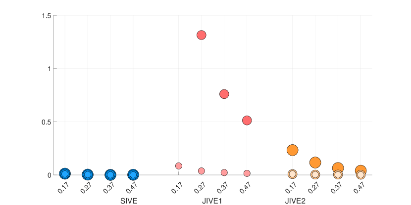
Figure 5: Average absolute bias in the estimand

Note: the figure shows the absolute median difference with the causal estimand in a setting without treatment heterogeneity. The size of the circles indicates the number of covariate groups with the small circle corresponding to $L=1$, the medium circle corresponding to $L=25$ and the large circle corresponding to $L=300$. The $x$-axis is the instrument strength $p(1)-p(0)$, with $p(0)=0.22$ and $p(1)=\{0.39,0.49,0.59,0.69\}$. Because JIVE1 shows large biases for $L=25$ and $L=300$, the $y$-axis is limited to $[0,0.9]$.

References

- Abadie (2003) Abadie, A. (2003). Semiparametric instrumental variable estimation of treatment response models. Journal of Econometrics 113(2), 231–263.
- Ackerberg and Devereux (2009) Ackerberg, D. A. and P. J. Devereux (2009). Improved JIVE estimators for overidentified linear models with and without heteroskedasticity. The Review of Economics and Statistics 91(2), 351–362.
- Angrist and Kolesár (2023) Angrist, J. and M. Kolesár (2023). One instrument to rule them all: The bias and coverage of just-id iv. Journal of Econometrics 0(just-accepted), 1–18.