Pump-efficient Josephson parametric amplifiers with high saturation power

Abstract

Circuit QED based quantum information processing relies on low noise amplification for signal readout. In the realm of microwave superconducting circuits, this amplification is often achieved via Josephson parametric amplifiers (JPA). In the past, these amplifiers exhibited low power added efficiency (PAE), which is roughly the fraction of pump power that is converted to output signal power. This is increasingly relevant because recent attempts to build high saturation power amplifiers achieve this at the cost of very low PAE, which in turn puts a high heat load on the cryostat and limits the number of these devices that a dilution refrigerator can host. Here, we numerically investigate upper bounds on PAE. We focus on a class of parametric amplifiers that consists of a capacitor shunted by a nonlinear inductive block. We first set a benchmark for this class of amplifiers by considering nonlinear blocks described by an arbitrary polynomial current-phase relation. Next, we propose two circuit implementations of the nonlinear block. Finally, we investigate chaining polynomial amplifiers. We find that while amplifiers with higher gain have a lower PAE, regardless of the gain there is considerable room to improve as compared to state of the art devices. For example, for a phase-sensitive amplifier with a power gain of 20 dB, the PAE is $\sim 0.1\%$ for typical JPAs, 5.9% for our simpler circuit JPAs, 34% for our more complex circuit JPAs, 48% for our arbitrary polynomial amplifiers, and at least 95% for our chained amplifiers.

I Introduction

The Josephson parametric amplifier (JPA) plays an important role in superconducting quantum computing. It uses the Josephson junction to amplify weak microwave signals with nearly quantum-limited added noise. Due to its ultralow-noise performance, the JPA is vital for readout [1, 2, 3, 4] for applications such as quantum state tomography [5], and, crucially, quantum error correction [6, 7, 8, 9].

A critical characteristic of the JPA is its ability to add the minimum noise throughout the parametric amplification process with a power gain of around 20 dB [10, 11, 12]. These noise and gain characteristics make JPAs suitable as the first stage of an amplifier chain, with the gain requirement being the minimum value to strongly saturate commercial cryogenic high electron mobility transistor (HEMT) amplifiers [12, 13]. Parametric amplification happens when the circuit’s parameter (e.g., inductance) is varied periodically at a specific frequency. In a microwave-pumped JPA, the periodic variation is achieved by using the nonlinearity of the Josephson junction to couple in a strong pump wave. Specifically, the nonlinearity mixes different frequency components; the pump wave at frequency $\omega_{\text{p}}$ and the signal wave at frequency $\omega_{\text{s}}$ mix and generate an idler wave at frequency $\omega_{\text{i}}=\omega_{\text{p}}-\omega_{\text{s}}$. The parametric process transfers energy from the pump wave to the signal and idler waves and thus amplifies the incoming signals [14, 15, 16].

Based on signal and idler frequencies, we usually classify the parametric amplifiers into phase-sensitive and phase-preserving amplifiers [12]. The phase-sensitive amplifier is also called the degenerate amplifier because its signal and idler frequencies are hosted in the same physical mode. Since the pump frequency is exactly twice the mode center frequency in this case, the power gain of the degenerate amplifier is sensitive to the relative phase between the pump and signal waves near the center of the amplifier’s mode frequency. In contrast, the phase-preserving amplifier, also known as the nondegenerate amplifier, has different signal and idler frequencies. In this case, the amplitude and phase information of the signal wave is maintained during the amplification process.

Besides added noise and gain, input saturation power and pump efficiency are also essential characteristics of the performance of parametric amplifiers [17, 18, 19, 20, 4]. The saturation power, $P_{\text{sat}}$, is defined as the smallest signal power at which the gain varies from the target gain $G_{\text{t}}$ by more than $\pm 1$ dB. As quantum computing systems scale up with more qubits, we need to process signals of various amplitudes. Thus, a large saturation power is desired since it enables us to read qubit states over a wide range of input powers without distortion. Older amplifier designs like Josephson parametric converters had relatively low saturation power. Surprisingly, the saturation power of these amplifiers was not limited by pump depletion. Instead, these amplifiers used a small number of Josephson junctions and, therefore, relatively small signal powers caused them to leave the desired nonlinear regime [21]. The newer generation of amplifiers splits the signal amplitude across many more Josephson junctions, thus resulting in a much larger saturation power [19, 22, 4].

The subject of this paper is pump efficiency, which characterizes the capacity of an amplifier to convert input power from the pump to output signal power without distorting the signal. Specifically, we use the power added efficiency (PAE) [23, p. 597], which is defined as

$$\eta_{\text{PAE}}(A_{\text{s}})=\frac{P_{\text{out}}-P_{\text{in}}}{P_{\text{pump}}}=\frac{(G(A_{\text{s}})-1)\omega_{\text{s}}^{2}A_{\text{s}}^{2}}{\omega_{\text{p}}^{2}A_{\text{p}}^{2}},$$ (1)

where $G(A_{\text{s}})$ is the power gain as a function of the input signal amplitude $A_{\text{s}}$, $A_{\text{p}}$ is the amplitude of the pump, and $\omega_{\text{s}}$ and $\omega_{\text{p}}$ refer to the signal and pump frequencies, respectively. Here, $P_{\text{in}}$ is the power of the input signal and $P_{\text{pump}}$ is the power of the pump wave. We note that $P_{\text{out}}$ consists only of the power being converted as output at the signal frequency, while ignoring the power at the idler frequency. Therefore, for phase-preserving amplifiers, but not phase-sensitive amplifiers, approximately half of the output power, which comes out at the idler frequency, is not accounted for in the PAE. We choose this definition because we expect that only the signal frequency will be used downstream. We also note that in this work, we will focus on amplifiers with a target gain of $G_{\text{t}}=20~{}\text{dB}$. Finally, we note that for convenience of the reader, we list commonly used symbols in Tab. 3.

We define the PAE of an amplifier, $\eta_{\text{PAE}}$, to be the maximum value of $\eta_{\text{PAE}}(A_{\text{s}})$ in the range of $A_{\text{s}}$ below saturation amplitude, $A_{\text{sat}}$. A higher PAE is desirable in JPAs used in large scale quantum computing applications to minimize heat load on the fridge. However, modern JPA designs tend to have pump efficiencies $(P_{\text{out}}/P_{\text{pump}})$ of less than $\sim$0.1% [20], indicating a huge gap between desired and actual performance levels.

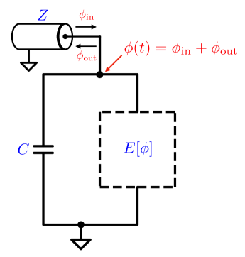
Figure 1: Generic amplifier circuit coupled to a transmission line with impedance $Z$. The circuit is composed of a capacitor $C$ and an inductive block with energy $E[\phi]$. The amplifier phase $\phi(t)$ is coupled to the transmission line via the input/output relation as indicated.

In this paper, we will investigate the ultimate limit on the PAE of a class of parametric amplifiers illustrated in Fig. 1. We will show that amplifiers within this class can have a PAE orders of magnitude higher than typical JPA designs. Specifically, we consider amplifier circuits of the general form shown in Fig. 1 that consist of a capacitor (denoted by $C$) in parallel with a nonlinear inductive block with energy $E[\phi]$. We first use this framework to explore the ultimate limit on PAE by considering arbitrary functions $E[\phi]$. Next, we explore buildable circuits where $E[\phi]$ represents the energy of a collection of inductors and Josephson junctions. Finally, we explore improving PAE by using amplifier chains. In the next three paragraphs, we summarize the results of these three directions.

To explore the ultimate limit on PAE, we begin by writing the energy of the inductive block of the amplifier as a generic polynomial

$$E[\phi]=\frac{1}{2L_{\text{eff}}}\phi^{2}+g_{3}\phi^{3}+g_{4}\phi^{4}+\cdots,$$ (2)

where $L_{\text{eff}}$ is the effective inductance of the inductive block. We tune the $g_{i}$ coefficients in this polynomial amplifier in order to maximize saturation power and, consequently, PAE. Searching through the space of polynomial amplifiers sets a bound on what level of efficiency is achievable given a certain order of nonlinearity, i.e., we can increase the PAE by adding further terms to $E[\phi]$. We have explored up to ninth order amplifiers. In Sec. III.1, we find that the PAE tends to saturate at around seventh order, where the maximum achievable PAE is at least 48% for degenerate amplifiers with $G_{\text{t}}=20~{}\text{dB}$.

Next, we investigate whether it is possible to achieve the same PAE from buildable amplifiers with inductive blocks composed of inductors and Josephson junctions. We replace the generic $E[\phi]$ by the energy of a circuit composed of these circuit elements. We choose circuits which have a comparable number of tuning parameters as in the polynomial case and adjust these parameters to optimize saturation power. In Sec. III.2, we show that we can reach a maximum PAE of 34% for degenerate amplifiers with $G_{\text{t}}=20~{}\text{dB}$.

Finally, we explore increasing PAE by chaining amplifiers. The PAE of an amplifier usually decreases as the gain increases. Therefore, one might expect to obtain an amplifier with a higher PAE by connecting several smaller gain amplifiers together. In Sec. III.3, we find that we can increase the PAE at $20$ dB from around $50\%$ to more than $95\%$ by chaining $\sim 30$ amplifiers (see in Fig. 21).

II Amplifier Model and Numerics

In this section, we lay out the model for a class of parametric amplifiers composed of a capacitor shunted by a nonlinear inductive block (shown in Fig. 2), derive the classical input-output relation, and obtain the equation of motion (EOM). Our calculations mainly follow Ref. 24.

II.1 Model

Here the amplifier is made of a capacitor and a nonlinear inductive block whose energy is $E[\phi]$. The Lagrangians of the amplifier, $\mathcal{L}_{\text{s}}$, and the transmission line, $\mathcal{L}_{\text{tl}}$, are

$$\mathcal{L}_{\text{s}} =\frac{C\dot{\phi}^{2}}{2}-E[\phi],$$ (3)

$$\mathcal{L}_{\text{tl}} =\sum_{i=1}\left(\frac{C_{l}\,\Delta x\,\dot{\phi}_{i+1}^{2}}{2}-\frac{({\phi_{i+1}}-{\phi_{i}})^{2}}{2L_{l}\,\Delta x}\right).$$ (4)

To couple the transmission line with the amplifier, we set $\phi_{1}=\phi$.

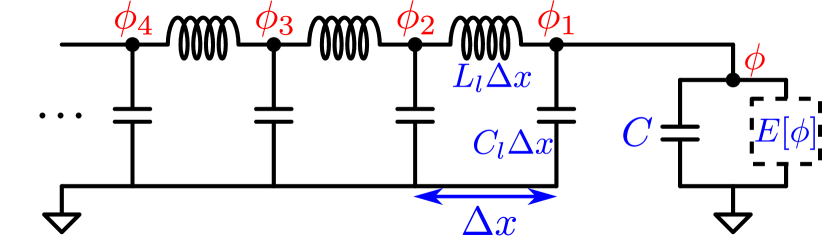
Figure 2: Schematic of the parametric amplifier with an explicit model for the transmission line, which we use to illustrate the origin of the input/output relations. Here, $\phi,\phi_{1},\phi_{2},\cdots$ are node fluxes in the transmission line; $C_{l},L_{l}$ are capacitance and inductance per unit length, respectively; $\Delta x$ is the cell length.

II.2 Equations of motion and input-output relations

We first consider the transmission line except for the last node $\phi_{1}$. For $i>1$, the equation of motion for $\phi_{i}$ is given by

$$\begin{aligned} C_{l}\,\Delta x\,\ddot{\phi}_{i}+\frac{{\phi_{i}}-{\phi_{i-1}}}{L_{l}\,\Delta x}-\frac{{\phi_{i+1}}-{\phi_{i}}}{L_{l}\,\Delta x}=0,\end{aligned}$$ (5)

which in the continuum limit, $\Delta x\to 0$, becomes the wave equation,

$$\ddot{\phi}+\frac{\phi^{\prime\prime}}{C_{l}L_{l}}=0,$$ (6)

where ^′ denotes the spatial derivative. We define the incoming and outgoing waves $\phi_{\text{in}}$ and $\phi_{\text{out}}$ such that

$$\left(\frac{\partial}{\partial t}+\frac{1}{\sqrt{C_{l}L_{l}}}\frac{\partial}{\partial x}\right)\phi_{\text{in}}=0,$$ (7)

$$\left(\frac{\partial}{\partial t}-\frac{1}{\sqrt{C_{l}L_{l}}}\frac{\partial}{\partial x}\right)\phi_{\text{out}}=0.$$ (8)

Then we have

$$\phi(x,t)=\phi_{\text{in}}(x,t)+\phi_{\text{out}}(x,t).$$ (9)

Next, we consider the boundary node flux $\phi_{1}=\phi$, which gives the input-output relation

$$\phi(t)=\phi(0,t)=\phi_{\text{out}}(0,t)+\phi_{\text{in}}(0,t).$$ (10)

The EOM of the boundary node flux is given by

$${C\ddot{\phi}}+J[\phi]=\frac{\phi^{\prime}|_{x=0}}{L_{l}}=\left.\frac{\dot{\phi}_{\text{in}}-\dot{\phi}_{\text{out}}}{Z}\right|_{x=0},$$ (11)

where $Z=\sqrt{L_{l}/C_{l}}$ is the characteristic impedance of the transmission line and $J[\phi]=\mathrm{d}E/\mathrm{d}\phi$ is the current through the inductive block as a function of the phase across the block, $\phi$. Together with the input-output relation (10), the evolution of the nonlinear system becomes

$$\ddot{\phi}+K\dot{\phi}+\frac{J[\phi]}{C}=2K\dot{\phi}_{\text{in}}|_{x=0},$$ (12)

where $K=\frac{1}{CZ}$ is the damping rate of the amplifier from its coupling to the transmission line.

II.2.1 Polynomial amplifiers

A polynomial amplifier of order $n$ is defined by a polynomial energy $E[\phi]=\frac{1}{2L_{\text{eff}}}\phi^{2}+g_{3}\phi^{3}+\cdots+g_{n}\phi^{n}$. The corresponding current-phase relation $J[\phi]$ is a polynomial of order $n-1$,

$$J[\phi]=\frac{1}{L_{\text{eff}}}\phi+3g_{3}\phi^{2}+\cdots+ng_{n}\phi^{n-1}.$$ (13)

The equation of motion for this amplifier is given by

$$\begin{aligned} \ddot{\phi}+K\dot{\phi}+\omega_{0}^{2}{\phi}+\frac{1}{C}(3g_{3}\phi^{2}+&\cdots+ng_{n}\phi^{n-1})\\ &={2K\dot{\phi}_{\text{in}}}|_{x=0},\end{aligned}$$ (14)

where $\omega^{2}_{0}=\frac{1}{CL_{\text{eff}}}$ is the natural frequency of the amplifier. We note that in this polynomial amplifier, the third order ($g_{3}$) term is primarily responsible for amplification. However, the third order term dynamically generates higher order nonlinear terms which limit the amplifier’s performance at high signal power [25, 21]. We aim to cancel the dynamically generated terms with higher order static terms in Eq. 14 in order to increase the saturation power and hence the PAE of the amplifier at fixed pump amplitude.

II.2.2 Josephson parametric amplifiers

In this subsection, we will discuss how to construct the inductive block $E[\phi]$ from linear inductors and Josephson junctions. We start from the Lagrangian description of inductors and Josephson junctions. The contributions of these elements to the energy $E[\phi]$ are

$$E_{L} =\frac{\phi_{0}^{2}}{2L}(\varphi_{1}-\varphi_{2})^{2},$$ (15)

$$E_{J} =-\phi_{0}i_{\text{c}}\cos(\varphi_{1}-\varphi_{2}),$$ (16)

where $E_{L},E_{J}$ are the contributions of inductors and Josephson junctions, respectively. Here, $L$ is inductance, $i_{\text{c}}$ is Josephson critical current, and $\phi_{0}$ is the reduced magnetic flux quantum. For JPAs we use dimensionless fluxes $\varphi_{i}=\phi_{i}/\phi_{0}$. In addition, we consider both current and flux biases in these circuits.

We represent the inductive block $E[\varphi]$ by a network of internal inductive components which make up our circuit design. Specifically, the circuit is composed of a set of internal nodes $\varphi_{i}$ that are connected by the inductive components. The inductive block does not contain any explicit dynamic terms since parasitic capacitances in this block are small and can be ignored. They are, however, sufficiently large that we operate in the singular regime of the Lagrangian, and thus we can neglect quantum effects as discussed in Ref. 26.

For each node $\varphi_{i}$, we write that $\frac{\partial\mathcal{L}}{\partial\varphi_{i}}=J_{i}=J_{\text{ext},i}$ where $J_{\text{ext},i}$ is the current bias at node $\varphi_{i}$. Typically, nodes are not current biased and thus have $J_{i}=0$. From here we proceed as in Ref. 21.

We also bias the circuit by applying external magnetic flux through closed loops in the circuit. Without loss of generality, we model magnetic flux bias by describing it as a phase offset across one of the Josephson junctions in the loop. In particular, a Josephson junction in a loop with an applied external flux of $\Phi_{\text{ext}}$ will have a contribution of $\frac{\phi_{0}^{2}}{2L}(\varphi_{1}-\varphi_{2}+\Phi_{\text{ext}})^{2}$ to the Lagrangian.

To make these considerations concrete, we examine the case of a JPA with an inductive block composed of $n\text{-many}$ radio frequency superconducting quantum interference devices (RF-SQUIDs) [27, 4, 28] as shown in Fig. 3. In this case, we need to describe only a single RF-SQUID since the flux $\varphi$ across the inductive block is divided equally among the $n$-many identical SQUIDs, and therefore each SQUID experiences a flux of $\frac{\varphi}{n}$. The resulting equation of motion is

$$\begin{aligned} \ddot{\varphi}+K\dot{\varphi}+\frac{\varphi}{nLC}+\frac{i_{\text{c}}}{C}\sin\left(\frac{\varphi}{n}+\Phi_{\text{ext}}\right)=2K\dot{\varphi_{\text{in}}},\end{aligned}$$ (17)

where $L$, $i_{\text{c}}$, and $\Phi_{\text{ext}}$ are the linear inductance, Josephson critical current, and external flux through each RF-SQUID, respectively. In general, we can construct the current-phase relation $J[\varphi]$ for the designed amplifier circuit and apply it to the EOM specified in equation (12).

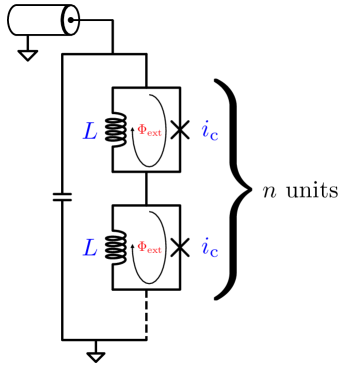
Figure 3: Amplifier circuit with an inductive block composed of a chain of $n$-many RF-SQUIDs. This type of circuit can have high saturation power, but it is limited to low PAE.

II.3 Numerical solutions of EOM and optimization algorithm for PAE

In this section, we provide the optimization algorithm that we use to maximize the PAE in the presence of the following incoming wave

$$\phi_{\text{in}}|_{x=0}=A_{\text{s}}\sin(\omega_{\text{s}}t)+A_{\text{p}}\sin(\omega_{\text{p}}t+\delta),$$ (18)

where $\omega_{\text{s}},\omega_{\text{p}}$ are the signal and pump frequencies, $A_{\text{s}},A_{\text{p}}$ are the signal and pump amplitudes, and $\delta$ is the phase difference between the signal and pump wave. Because the differential equation (14) is nonlinear, inhomogeneous and non-autonomous, obtaining analytical solutions is not possible in general. Thus, we first introduce two numerical methods, the direct time integration (DTI) and the harmonic balance (HB) method, that we use to solve this differential equation.

The DTI method is based on numerical integration techniques that approximate the differential equation by using finite differences. The DTI method uses function values and finite differences at current and previous time intervals to find the value at the next interval. In our calculation, we use the Python method scipy.integrate.odeint to solve the nonlinear differential equation [29]. Since we want to obtain a steady-state solution, we choose our integration time to be at least 2000 periods of the signal wave. Then, to remove the initial transient, we only analyze the data from the last quarter of the integration time. After obtaining the solution in the time domain, we apply the Discrete Fourier Transform (DFT) to isolate the outgoing signal wave from the rest of the solution. This requires the last quarter of the integration time to be a multiple of $T_{\min}=\gcd(\frac{2\pi}{\omega_{\text{s}}},\frac{2\pi}{\omega_{\text{p}}})$ which dictates our choice of $\omega_{\text{p}}/\omega_{\text{s}}$. Finally, the PAE is determined by calculating both the saturation power gain and the amplitude of the signal wave at that gain.

The HB method exploits the periodicity of the external driving force and solves the differential equation in the frequency domain. If the incoming wave $\phi_{\text{in}}$ is periodic with a period of $T$, then the solution to Eq.(14) is also periodic with the same period $T$. Thus, we can propose that the solution to Eq. (14) takes the following form (in the degenerate case):

$$\phi(t)=a_{0}+a_{1}e^{i\omega_{0}t}+\cdots+a_{n}e^{in\omega_{0}t}+h.c..$$ (19)

Then, the solution can be obtained by matching coefficients on both sides of Eq. (14). To ensure we have chosen a sufficiently large $n$, we also compare the HB method with the DTI method. For degenerate amplifiers, the HB method is typically much faster than the DTI method. On the other hand, for nondegenerate amplifiers, we need to consider many more harmonics in the HB method. In this case, the DTI method is faster, and is the one we use. A more comprehensive analysis of these methods is provided in Appendix B.

Before we describe the optimization algorithm, we normalize the EOM by rescaling time and flux. By doing so, we reduce the number of parameters in the differential equation, making it easier to work with. The initial differential equation is

$$\ddot{\phi}+K\dot{\phi}+\omega_{0}^{2}{\phi}+\frac{1}{C}(3g_{3}\phi^{2}+\cdots+ng_{n}\phi^{n-1})={2K\dot{\phi}_{\text{in}}},$$ (20)

with the incoming wave $\phi_{\text{in}}=A_{\text{s}}\sin(\omega_{\text{s}}t)+A_{\text{p}}\sin(\omega_{\text{p}}t+\delta)$. First, we rescale time $t\to t/\omega_{0}$, i.e. we work in units where $\omega_{0}=1$. Next, we scale flux so that $A_{\text{p}}$ is normalized to be $0.5$. In this case, the pump power is $\omega_{\text{p}}^{2}$, and the PAE is $4(G-1)A_{\text{s}}^{2}\omega_{\text{s}}^{2}/\omega_{\text{p}}^{2}$. Finally, we rescale coefficients $g_{i}$ to absorb $1/C$. In the following, we will use the same letter to denote the normalized polynomial coefficients. After rescaling, our differential equation becomes

$$\ddot{\phi}+K{\dot{\phi}}+{\phi}+3g_{3}\phi^{2}+\cdots+ng_{n}\phi^{n-1}=2K\dot{\phi}_{\text{in}},$$ (21)

with the incoming wave $\phi_{\text{in}}=A_{\text{s}}\sin(\frac{\omega_{\text{s}}}{\omega_{0}}t)+\frac{1}{2}\sin(\frac{\omega_{\text{p}}}{\omega_{0}}t+\delta)$.

While we wish to maximize the PAE of the amplifier directly, this is difficult, and therefore we use a proxy. Specifically, we minimize the difference between the amplifier gain and $G_{\text{t}}$ over the largest possible range of $A_{\text{s}}$. We take the highest PAE below the saturation power of the amplifier as the amplifier’s PAE. This maximum PAE typically occurs at or near the saturation power of the amplifier (see in Fig. 4). The optimization variables we use are $K,g_{3},g_{4},\cdots$. In the remainder of this section, we will present the algorithm step by step with necessary explanations. A pictorial demonstration of the algorithm is also provided in Fig. 5.

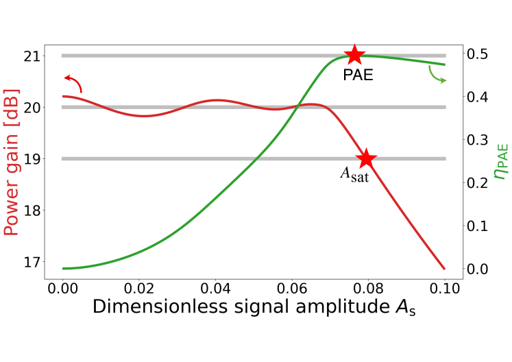
Figure 4: Power gain and PAE versus dimensionless signal amplitude $A_{\text{s}}$ of a 7-th order 20 dB degenerate amplifier. The parameters of this amplifier can be found in Tab. 4. The saturation amplitude $A_{\text{sat}}$ is the signal amplitude where the gain curve intersects the $G_{\text{t}}\pm 1$ dB lines. The PAE of an amplifier is defined to be the maximum PAE below the saturation power, which typically appears at or around $A_{\text{sat}}$.

Step 1. Choose an initial range $[0,R]$ for $A_{\text{s}}$, and a set of initial variables $\{K^{(0)}$, $g_{3}^{(0)}$, $g_{4}^{(0)},\cdots\}$. This set of variables generates an initial gain curve as shown in Fig. 5(1).

Step 2. Divide the region $[0,R]$ into $N$ sub-intervals and define the cost function $f$ as the sum of the squared distance as illustrated in Fig. 5(2).

$$\begin{aligned} &f\left(K^{(0)},g_{3}^{0},g_{4}^{(0)},\cdots\right)\stackrel{{\scriptstyle\mathrm{def}}}{{=}}\\ &\sum_{m=1}^{N}\left(G\left(A_{\text{s}}=\frac{mR}{N},K^{(0)},g_{3}^{(0)},g_{4}^{(0)},\cdots\right)-G_{\text{t}}\right)^{2}.\end{aligned}$$ (22)

Step 3. Minimize the cost function $f$ using the gradient descent algorithm. By doing so, we will get a new collection of coefficients $\{K^{(1)}$, $g_{3}^{(1)}$, $g_{4}^{(1)},\cdots\}$.

Step 4. Calculate the saturation point for the new curve, which is shown in Fig. 5(4), and reset the new range to be $[0,A_{\text{sat}}]$ if $A_{\text{sat}}$ exceeds the previous range $R$; otherwise, stop the optimization.

Step 5. Redefine the cost function $f$ within the new range as depicted in Fig. 5(5), and repeat steps 3 to 5 until the optimization stops.

Step 6. Record the optimized values of the amplifier parameters $K,g_{3},g_{4},\cdots$.

The solution and optimization of amplifiers described by circuits is similar to the description above, and we provide details of this procedure in Appendix C.

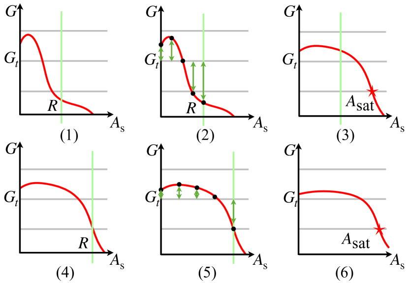
Figure 5: Schematic of optimization algorithm steps. (1) Start from an initial optimization range $[0,R]$ and a set of initial variables $\{K^{(0)},g^{(0)}_{3},g^{(0)}_{4},\cdots\}$. (2) Calculate the cost function corresponding to the green arrows. (3) Minimize the cost function. (4)-(5) Update the optimization range $[0,R]$ and re-optimize the amplifier’s coefficients until the optimization process stops. (6) Record the optimal values of the amplifier parameters $\{K,g_{3},g_{4},\cdots\}$.

III Results

III.1 Polynomial amplifiers

In this subsection, we apply our optimization algorithm to the polynomial amplifier to find a lower bound on the maximum PAE for the class of amplifiers that we consider in Fig. 2. The goal of this subsection is to set a benchmark that we will attempt to match in the next subsection with amplifiers that can be expressed as circuits. We first focus on degenerate amplifiers where $2\omega_{\text{s}}=\omega_{\text{p}}$. We fix the relative phase $\delta$ to be $1.5\pi$. This choice tends to maximize the gain in the small signal regime. We will start by establishing how the PAE depends on the order of the polynomial by optimizing a set of amplifiers with different orders to the target gain of 20 dB. We will choose the polynomial order that balances the algorithm’s run time and amplifier performance. Next, we will fix the polynomial order and vary the target gain to determine the relation between target gain and PAE. Finally, we will switch our focus to nondegenerate amplifiers and determine the dependence of PAE on target gain.

We start by optimizing the PAE of $20~{}\text{dB}$ degenerate polynomial amplifiers with order varying from 3 to 9. The outcomes of this process are illustrated in Fig. 6. To avoid local optima, we repeat our optimization algorithm with different starting points multiple times for each target gain and keep the highest PAE. We observe that as we increase the polynomial order from 3 to 9, the saturation power $A_{\text{sat}}$ of these amplifiers improves significantly, rising from about 0.01 to around 0.08, corresponding to a rise in PAE from approximately 1% to almost 50%. We note that the PAE saturates at around the seventh order (see in Tab. 1). So, we focus on the performance of the 7th-order polynomial amplifier in this section.

polynomial order	dimensionless $A_{\text{sat}}$	PAE
3	0.0125	12.3%
4	0.0143	16.1%
5	0.0577	26.2%
6	0.0728	41.3%
7	0.0794	48.4%
8	0.0801	48.3%
9	0.0794	48.2%

Table 1: Saturation amplitude $A_{\text{sat}}$ and PAE of optimized 20 dB polynomial amplifiers with different orders of nonlinearity. Parameters of the amplifiers can be found in Tab. 4.

Next, we sweep the target gain of the 7th-order polynomial degenerate amplifiers from 1.2 dB to 26 dB. As depicted in Fig. 7, there is a gradual decline in the PAE, dropping from nearly 100% at 1.2 dB to about 40% at 26 dB. As before, we use multiple starting points for the optimization algorithm. In Fig. 7 we plot all the resulting PAEs. At lower target gains, different starting points generally yield similar PAEs. However, in the high gain regime, we observe that the algorithm’s output begins to fluctuate (see Fig. 7), with some amplifiers tending to be trapped in local optima, as shown in Fig. 8.

We used the optimal points of the degenerate amplifiers as starting points for the optimization of the nondegenerate amplifiers. The reason for this choice, as opposed to using a large number of random starting points, was that the large computational complexity of characterizing nondegenerate amplifiers made trying a large number of starting points computationally too expensive. We remind the reader that characterizing nondegenerate amplifiers is computationally much more expensive than characterizing degenerate amplifiers because the former requires the use of the direct time integration method while the latter can be much more efficiently handled by the harmonic balance method. Even within the context of the direct time integration method, nondegenerate amplifiers require longer integration time since $T_{\min}$ is large. This is due to the slight offset of the signal frequency from half the pump frequency, which increases $\gcd(\frac{2\pi}{\omega_{\text{s}}},\frac{2\pi}{\omega_{\text{p}}})$.

For the case of degenerate amplifiers, we previously observed a steady decline of the PAE with increasing target gain (see Fig. 7). On the other hand, for the case of nondegenerate amplifiers we observe that as we sweep the target gain, the PAE does not strongly depend on the target gain except for the lowest target gain point (see Fig. 9). It is possible that this behavior, i.e. lower than expected PAE at intermediate target gain, is a consequence of our choice of starting points for our optimization procedure. To try to address this possibility, we attempted to extend the optimal solution of the lowest target gain point to higher target gains. Unfortunately, we found that this was a poor choice of starting point at higher target gains as it resulted in amplifiers with large amplitude ripple, and therefore low PAE.

At high target gain, we did find nondegenerate amplifiers with reasonable performance. Indeed, for a 20 dB amplifier, we achieved a PAE of 14% (see Fig. 9). We remind the reader that our definition of PAE only accounts for the power leaving the amplifier at the signal frequency and not the idler frequency.

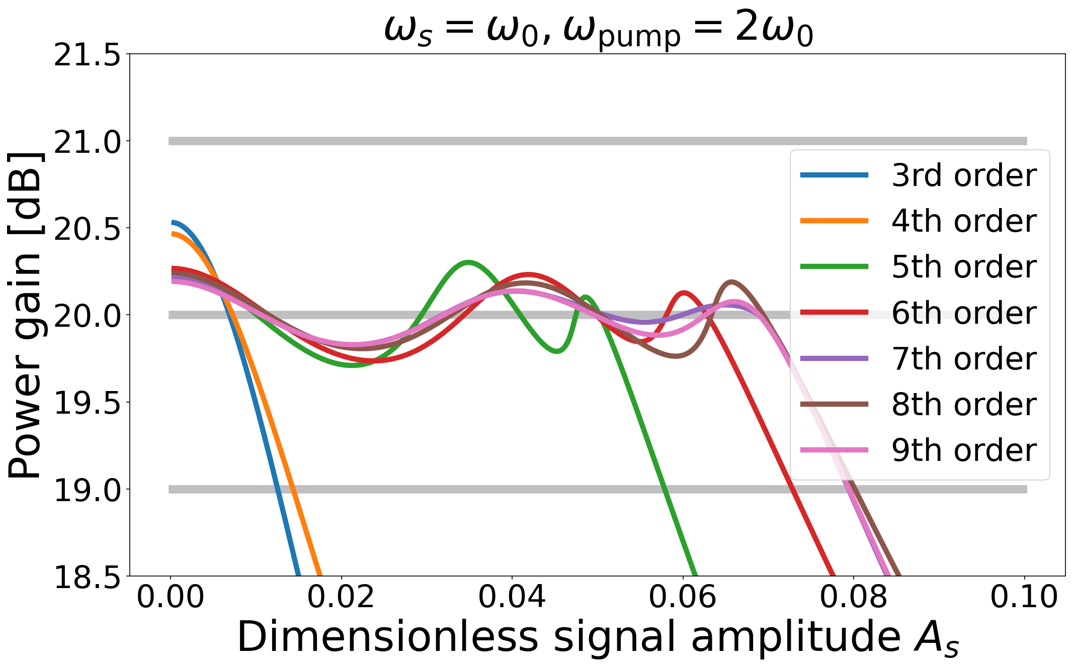
Figure 6: Power gain versus dimensionless signal amplitude curves for optimized 20 dB polynomial amplifiers with different orders of nonlinearity. Parameters of these amplifiers are listed in Tab. 4.

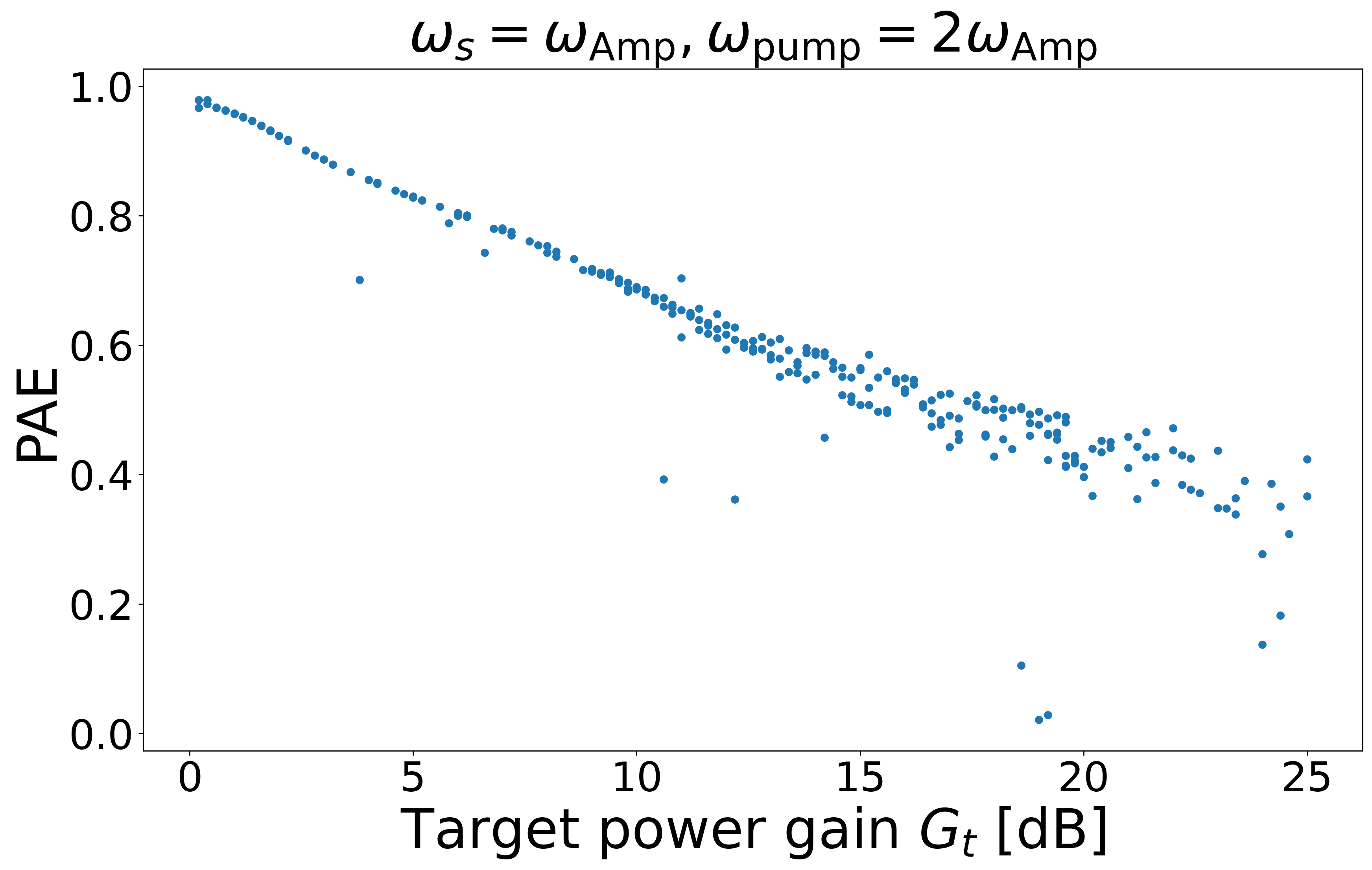
Figure 7: PAE versus target gain of $7$-th order polynomial degenerate amplifiers, showing that PAE generally decreases as amplifier gain increases.

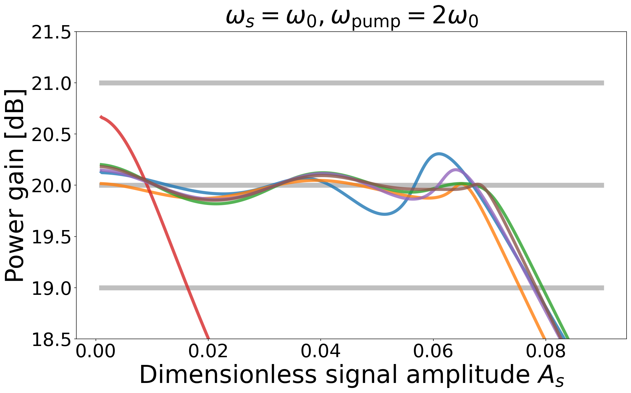
Figure 8: Importance of initial points to optimization results. Here, we show gain versus signal amplitude curves of 20 dB $7$-th order polynomial amplifiers, where different curves represent amplifiers that were found by optimizing from six different starting points.

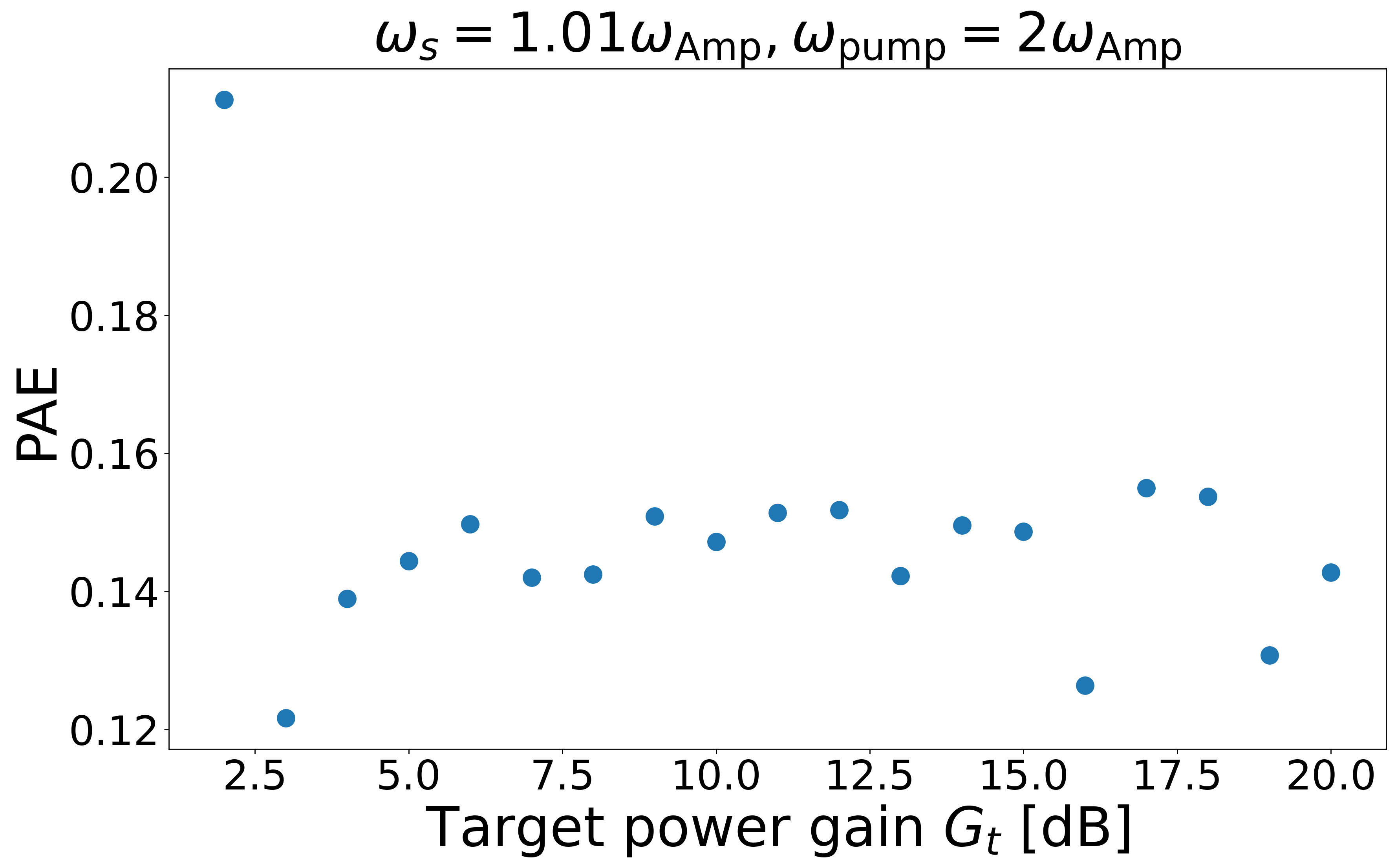
Figure 9: Pump efficiency as a function of target gain for $7$-th order polynomial nondegenerate amplifiers.

III.2 JPA circuits

In this subsection we will examine JPA circuits which are optimized to a target gain of $G_{\text{t}}=20~{}\text{dB}$, which is a common target in quantum computing applications. We will do so in both the degenerate and nondegenerate cases. We will first provide amplifiers with the highest possible PAE, where all circuit parameters as well as the damping rate $K$ are optimized. These high PAE amplifiers, however, may prove impractical to build due to high $K$ and complexity of the resulting circuit design. We will then provide JPA designs which are more likely to be buildable with modern techniques. In addition to amplifier gain, we provide bandwidth and third order intercept point (IP3) characteristics for our nondegenerate amplifier designs.

III.2.1 Highest PAE amplifiers

We find that by using JPA circuit designs, we are able to achieve a PAE almost as high as the optimized polynomial amplifiers. Specifically, we investigate amplifiers with inductive blocks composed of RF-SQUIDs shunted by three Josephson junctions in series with an applied current bias, as well as a separate flux bias through the RF-SQUID loop, as shown in Fig. 10. By tuning circuit parameters, we can achieve 20 dB gain up to a high maximum signal power. This is possible in the degenerate case, where $\omega_{\text{p}}=2\omega_{\text{s}}$, as well as in nondegenerate cases.

In the degenerate case, we were able to optimize our amplifiers to a PAE of 34.0%. We plot the gain of this amplifier as a function of signal power in Fig. 11. In the nondegenerate case, we get a PAE of approximately 11.8%, with the gain curve shown in Fig. 13. These circuits have parameters as listed in Tab. 2. We note that our optimization is independent of the choice of capacitance $C$, and so our circuit elements and pump power can be rescaled by a different choice of $C$. In particular, inductances (e.g., $L$ and $L_{1}$) are inversely proportional to $C$, while currents (e.g., $i_{c1},i_{c2},$ and $J_{\text{ext}}$) and pump power, $P_{\text{pump}}$, are directly proportional to $C$. Here, we choose $C=0.5$ pF and provide device parameters based on this choice.

In Fig. 12 we demonstrate how increasing damping rate allows us to optimize amplifiers for higher PAE. Here, we provide the PAE of degenerate amplifiers of various damping rates, each with 25 copies of our extended RF-SQUID, optimized to highest saturation power. The resulting PAE of each amplifier increases monotonically with damping rate.

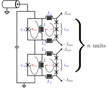
Figure 10: Amplifier circuit design which gives highest PAE. The circuit is composed of $n$-many RF-SQUIDs, each shunted by 3 current-biased Josephson junctions.

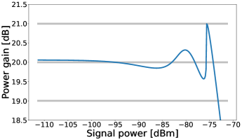
Figure 11: Gain versus input signal power of the degenerate amplifier shown in Fig. 10, with optimized circuit tuned to 20 dB gain. Parameters for this amplifier are listed in Tab. 2.

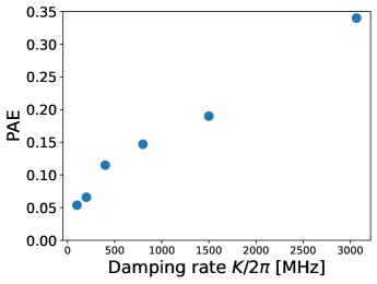
Figure 12: PAE of degenerate amplifiers with circuits as shown in Fig. 10. Each amplifier is optimized with a different damping rate, demonstrating increasing PAE with higher damping rate.

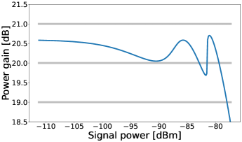
Figure 13: Gain versus input signal power of the nondegenerate amplifier shown in Fig. 10, with optimized circuit tuned to 20 dB gain. Parameters for this amplifier are listed in Tab. 2. The signal frequency is $\omega_{\text{s}}=125/249\omega_{\text{p}}$.

parameter	degenerate	nondegenerate	more practical degenerate	more practical nondegenerate
$P_{\text{pump}}$	-49.5 dBm	-49.5 dBm	-53.3 dBm	-53.0 dBm
$n$	25	25	10	25
$K$	3.07 $(2\pi)$ GHz	3.08 $(2\pi)$ GHz	0.8 $(2\pi)$ GHz	0.8 $(2\pi)$ GHz
$C$	0.5 pF	0.5 pF	0.5 pF	0.5 pF
$i_{\text{c1}}$	15.6 $\mu$A	16.1 $\mu$A	0.730 $\mu$A	3.36 $\mu$A
$i_{\text{c2}}$	9.07 $\mu$A	9.11 $\mu$A	4.67 $\mu$A	1.45 $\mu$A
$L$	79.4 pH	82.6 pH	217 pH	53.8 pH
$L_{1}$	83.0 pH	88.6 pH	0.4 pH	0.784 pH
$\Phi_{\text{ext}}$	5.72 $\phi_{0}$	5.67 $\phi_{0}$	0.472 $\phi_{0}$	4.15 $\phi_{0}$
$J_{\text{ext}}$	0.100 $\mu$A	0.100 $\mu$A	-5.26 $\mu$A	0.394 $\mu$A

Table 2: Optimized amplifier circuit parameters. Degenerate and nondegenerate columns refer to circuits as shown in Fig. 10, while more practical degenerate and more practical nondegenerate columns refer to circuits as shown in Fig. 14. We optimize with $n=25$ in each case except the more practical degenerate amplifier. In this case it proved difficult to optimize with $n=25$ and so instead we used $n=10$.

III.2.2 More practical amplifiers

While the amplifiers above have high PAEs, there remain two main challenges in physically realizing amplifiers with these designs. First is the high damping rate of $K/2\pi\approx 3$ GHz, and second is the use of $n$-many independent current sources. Here we present a simpler circuit with lower $K$ and only a single current source.

This more practical design is illustrated in Fig. 14. Parameter values that optimize this circuit for 20 dB gain can be found in Table 2. We provide parameters for both the degenerate and nondegenerate cases, with their respective gain curves plotted in Fig. 15 and Fig. 16. The PAE of the degenerate amplifier is approximately 5.91%, while that of the nondegenerate amplifier is 2.37%.

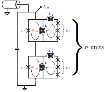
Figure 14: Amplifier circuit with a more practical design. The circuit is composed of $n$-many RF-SQUIDs, each shunted by 3 Josephson junctions with a single overall current bias.

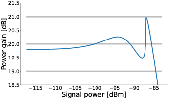
Figure 15: Gain versus input signal power of a degenerate amplifier with a more practical circuit as shown in Fig. 14, tuned to 20 dB gain. Parameters for this amplifier are listed in Tab. 2.

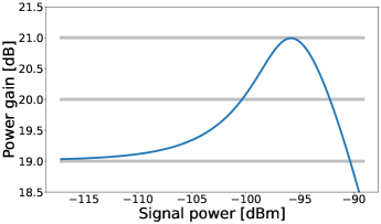
Figure 16: Gain versus input signal power of a nondegenerate amplifier with a more practical circuit as shown in Fig. 14, tuned to 20 dB gain. Parameters for this amplifier are listed in Tab. 2. The signal frequency is $\omega_{\text{s}}=125/249\omega_{\text{p}}$.

III.2.3 Bandwidth and IP3

Bandwidth is an important measure of amplifier performance due to the need to amplify signals over a range of frequencies. For the amplifiers in subsection III.2.1, we find a bandwidth of 279 MHz. The large bandwidth is a consequence of the high damping rate of about 3 GHz. We plot the gain of the nondegenerate amplifier over a range of frequencies in Fig. 17(a), demonstrating this bandwidth. The gain versus signal frequency plot for the nondegenerate amplifier described in subsection III.2.2 is shown in Fig. 17(b), with a bandwidth of 97 MHz.

Another measure of amplifier performance is IP3, which indicates the range of signal power over which intermodulation products between two distinct signal frequencies remain small. Here, we compute the output power of third order intermodulation products resulting from the amplification of two similar but distinct signal frequencies within the amplifier bandwidth [23, p. 511-518]. We note that in order to reduce computation run time, we slightly modify the procedure in subsection II.3 to use the last half of the DTI solution rather than the last quarter, while ensuring the integration time remains at least 2000 periods of the signal frequencies. This allows us to choose an integration time which is twice $T_{\text{min}}$ rather than 4 times $T_{\text{min}}$. This reduced integration time does not affect our solution since for the two similar signal frequencies used in IP3 analysis, the integration time is very long and transient solutions die out far before half the integration time.

We provide a diagram of the output power of our two signals as well as third order products in Fig. 18(a), which demonstrates the IP3 performance of the amplifier in subsection III.2.1. As anticipated, the output signal power grows linearly with input signal power, while the third order terms grow cubically until the saturation point. We find IIP3 of $-79.2$ dBm and OIP3 of $-62.3$ dBm. Similarly, in Fig. 18(b), we provide the IP3 performance of the amplifier in subsection III.2.2, where we find IIP3 of $-88.7$ dBm and OIP3 of $-75.7$ dBm.

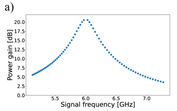
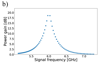
Figure 17: Amplifier bandwidth: gain of the amplifier versus signal frequency. a) Amplifier in subsection III.2.1 b) Amplifier in subsection III.2.2.

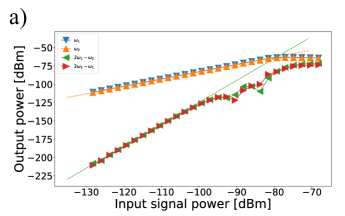
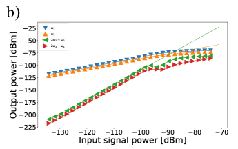
Figure 18: IP3: output power of signal frequencies as well as their third order intermodulation products, plotted in dBm units. Here we have $\omega_{1}=101/201\omega_{\text{p}}$ in blue and $\omega_{2}=101/200\omega_{\text{p}}$ in orange. The third order term $2\omega_{1}-\omega_{2}$ is in green and $2\omega_{2}-\omega_{1}$ is in red. We include linear fits for $\omega_{2}$ and $2\omega_{1}-\omega_{2}$ which demonstrate the intercept points. These fits take into account the 3rd through 10th points of each data set. a) Amplifier in subsection III.2.1 b) Amplifier in subsection III.2.2.

III.3 Chained polynomial amplifiers

Polynomial amplifiers always have a higher PAE at relatively low target gains (as shown in Fig. 7). Intuitively, without introducing extra higher order nonlinearity, we can obtain a higher PAE by connecting amplifiers with smaller gains as opposed to a single amplifier with higher gain. In this section, we first calculate the total PAE for a chained amplifier consisting of two amplifiers. Next, we use the result from Sec. III.1 to show that we can increase the total PAE significantly by tuning the gain of the two amplifiers. Finally, we extend our investigation to a chain of $n$ amplifiers that all have the same gain and PAE. These amplifiers are not identical, as $A_{\text{sat}}$ needs to be appropriately scaled to match the signal amplitude in the amplifier chain. By connecting approximately 30 amplifiers in a chain, we can achieve a PAE of 95% for a 20 dB degenerate amplifier.

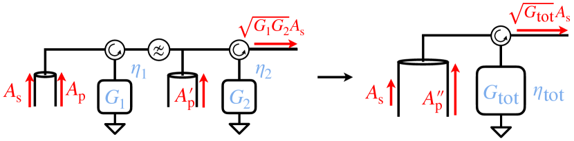
Figure 19: A schematic of an amplifier chain. Circulators and low-pass filters are added to route input, output, and pump waves.

We start by considering the case where two amplifiers are connected as shown in Fig. 19. These amplifiers operate at gains of $G_{1}$ and $G_{2}$, and achieve PAEs of $\eta_{1}$ and $\eta_{2}$, respectively. Let $A_{\text{s}}$ denote the amplitude of the input signal wave, and let $A_{\text{p}}$ and $A_{\text{p}}^{\prime}$ denote the amplitudes of the two pump waves, respectively. The total gain and the total PAE for this amplifier chain, denoted as $G_{\text{tot}}$ and $\eta_{\text{tot}}$, are given by

$$G_{\text{tot}}=G_{1}G_{2}, \eta_{\text{tot}}=\frac{(G_{1}G_{2}-1)\omega_{\text{s}}^{2}A_{\text{s}}^{2}}{\omega_{\text{p}}^{2}{A_{\text{p}}^{\prime}}^{2}+\omega_{\text{p}}^{2}A_{\text{p}}^{2}}.$$ (23)

Recalling the definitions of $\eta_{1}$ and $\eta_{2}$,

$$\eta_{1}=\frac{(G_{1}-1)\omega_{\text{s}}^{2}A_{\text{s}}^{2}}{\omega_{\text{p}}^{2}A_{\text{p}}^{2}}, \eta_{2}=\frac{G_{1}(G_{2}-1)\omega_{\text{s}}^{2}A_{\text{s}}^{2}}{\omega_{\text{p}}^{2}{A_{\text{p}}^{\prime}}^{2}},$$ (24)

we obtain

$$\begin{aligned} \eta_{\text{tot}}=\frac{G_{1}G_{2}-1}{\frac{G_{1}-1}{\eta_{1}}+\frac{G_{1}(G_{2}-1)}{\eta_{2}}}.\end{aligned}$$ (25)

The PAE of the combined amplifier chain is bounded by the PAE of each individual amplifier,

$$\min(\eta_{1},\eta_{2})\leq\eta_{\text{tot}}\leq\max(\eta_{1},\eta_{2}),$$ (26)

and is determined by how the gain is split between two amplifiers. These results can be easily generalized to the $n$-amplifier case, where we have

$$G_{\text{tot}}=\prod_{i}G_{i}, \eta_{\text{tot}}=\frac{G_{\text{tot}}-1}{\sum_{i}\frac{G_{i}-1}{\eta_{i}}\prod_{k<i}G_{i}}.$$ (27)

For a chain of amplifiers that have the same power gain of $G$ and a PAE of $\eta_{\text{PAE}}$, the total gain is $G_{\text{tot}}=G^{n}$, and the total PAE is simply $\eta_{\text{tot}}=\eta_{\text{PAE}}$.

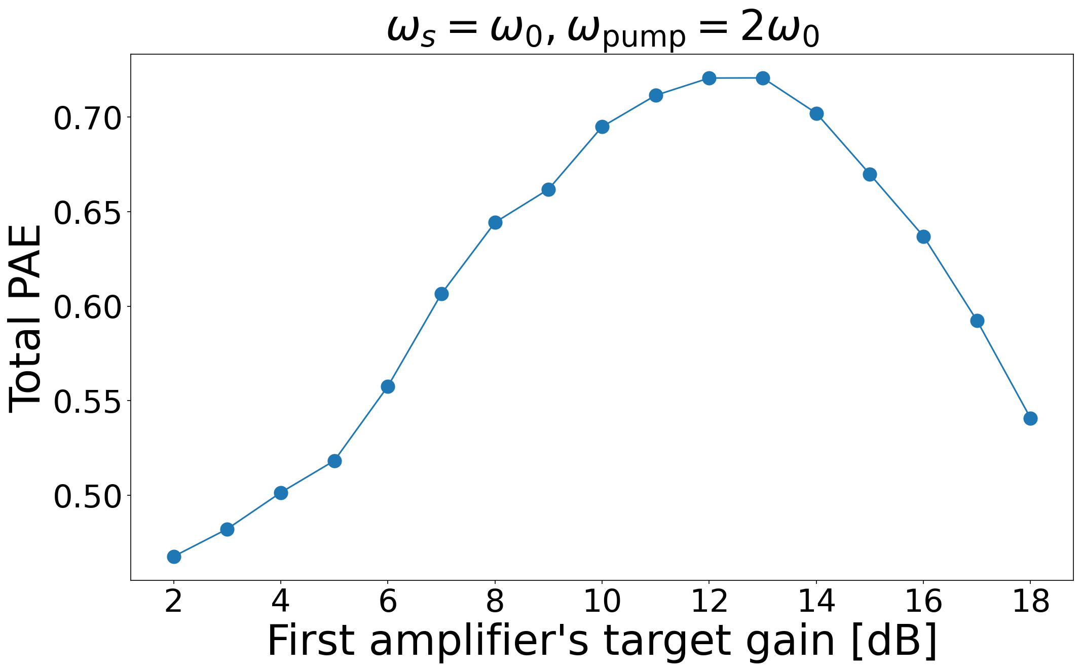
Figure 20: Total PAE of a chained 20 dB degenerate amplifier consists of two 7-th order polynomial amplifiers.

In subsection III.1, we optimized a range of polynomial amplifiers designed for various target gains. Specifically, for a target gain of $G_{\text{t}}=20$ dB, the highest PAE we obtained was $48.4\%$. To improve this efficiency, we connect a pair of smaller gain amplifiers to achieve a total gain of 20 dB with overall threshold $\pm 1$ dB. To characterize the amplifier chain, we used the PAE versus gain curve from Fig. 7. To ensure the overall gain variation does not break the $\pm 1$ dB threshold, we made sure that each amplifier in the chain does not break a threshold of $\pm 0.5$ dB. The performance of this amplifier chain is illustrated in Fig. 20. We observe that the total PAE of the chain peaks at 72% when the first amplifier is set to a gain of 13 dB and the second to a gain of 7 dB.

We now extend our analysis to a chain of $n$ amplifiers with each amplifier having the same target gain and PAE. We put a threshold of $\pm 1/n$ dB on each amplifier. As we increase the number of amplifiers from 1 to 28, the total PAE gradually increases from$~{}50\%$ to$~{}95\%$, as presented in Fig. 21. Extrapolating from Fig. 7, we anticipate that the total PAE would eventually approach 100% as $n\!\to\!\infty$.

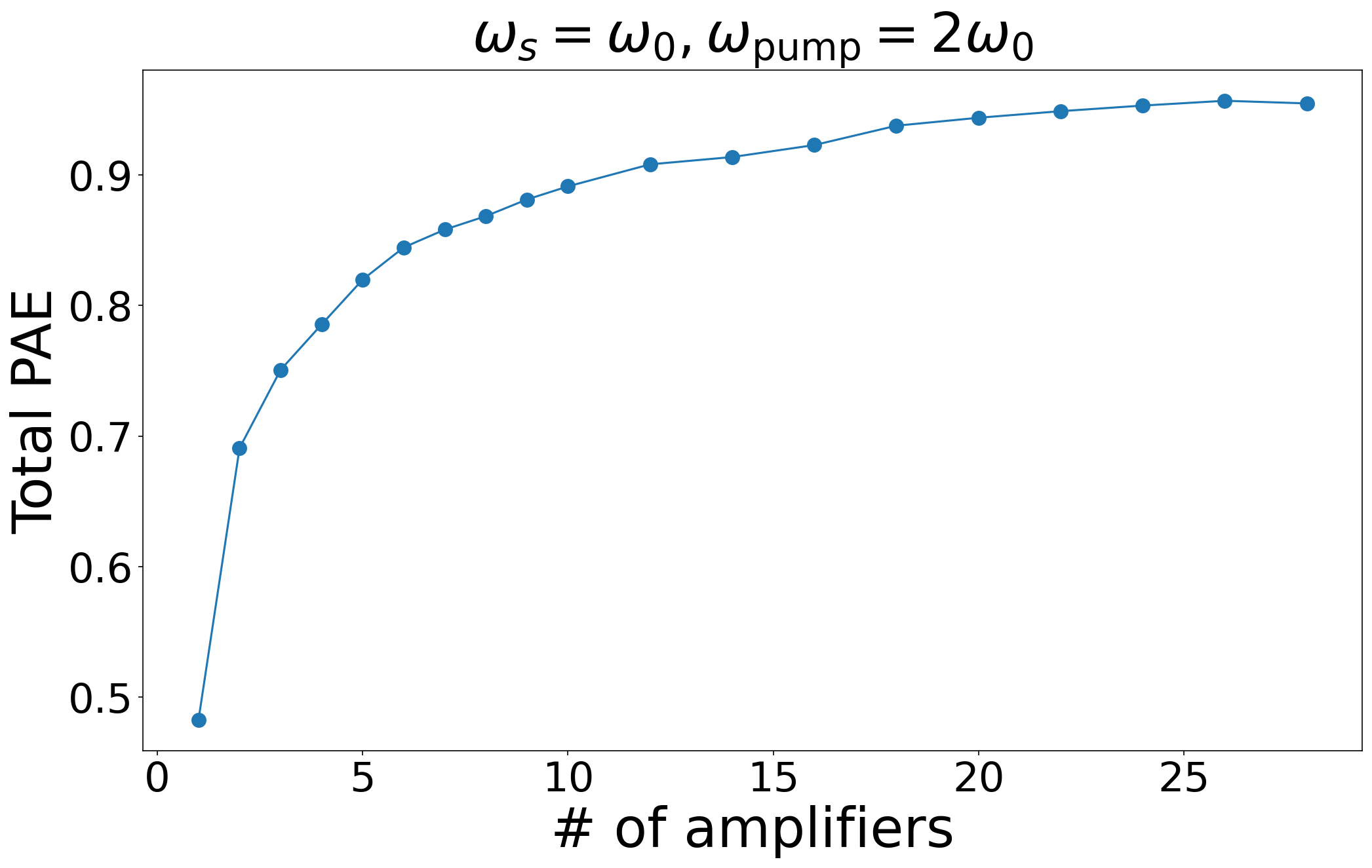
Figure 21: Total PAE of a chained 20 dB degenerate amplifier consisting of $n$ same-performance amplifiers.

IV Discussion

Due to the limited power added efficiency of modern JPAs and the need for low noise, efficient amplifiers in quantum computing applications, we have explored optimizing JPA designs by finely tuning the amplifier’s Hamiltonian. We find that with the freedom to define an arbitrary inductive block, we can design amplifiers with a PAE orders of magnitude higher than that of modern JPAs. Using polynomial amplifier designs, we find that we can reach a PAE of nearly 50% at 20 dB gain, which is the upper limit in the nondegenerate case.

Furthermore, restricting ourselves to inductive blocks consisting of circuits extending previous RF-SQUID designs, we still realize a significant improvement in PAE. We are able to design JPA circuits with high PAEs, large bandwidth, and limited intermodulation distortion. We also provide designs for amplifiers with reduced PAE which may prove to be more practically buildable. These amplifiers could prove to be useful in quantum computing applications which require the amplifier to be located in proximity to qubits at millikelvin temperatures, where minimizing heat dissipation is a priority. We anticipate many, or at least several, of these devices to be mounted in a single dilution refrigerator. Recent implementations of low-PAE, high-saturation power amplifiers are problematic [22, 28] due to the extremely high pump powers utilized in these experiments, which in turn generate excessive heat in the cryostat.

Finally, by considering chains of polynomial amplifiers, we explore the maximum possible PAE for degenerate amplification. We note that by increasing the number of amplifiers in our chain, we are able to achieve a higher PAE which tends to 100%. We believe that the advances in theoretically achievable PAE which we outline here can serve as a basis for future parametric amplifiers with use cases where reduced power consumption and dissipation are essential.

Appendix A Additional Tables

symbol	meaning
$\phi$	node flux of the amplifier
$\phi_{0}=\hbar/2e$	reduced magnetic flux quantum
$\varphi=\phi/\phi_{0}$	dimensionless node flux of the amplifier
$\phi_{\text{in}},\phi_{\text{out}}$	incoming and outgoing waves on transmission line
$\Phi_{\text{ext}}$	external magnetic flux
$C_{l},L_{l}$	capacitance and inductance per unit length of the transmission line
$Z=\sqrt{L_{l}/C_{l}}$	characteristic impedance of the transmission line
$\mathcal{L}_{\mathrm{s}},\mathcal{L}_{\text{tl}}$	Lagrangians for the amplifier and transmission line
$E[\phi]$	energy of the inductive block of the amplifier
$J[\phi]={\mathrm{d}E[\phi]}/{\mathrm{d}\phi}$	current-phase relation of the inductive device
$A_{\text{s}},A_{\text{p}}$	incoming signal/pump wave amplitudes
$\omega_{\text{s}},\omega_{\text{p}}$	incoming signal/pump wave frequencies
$\delta$	phase difference between the signal and pump waves
$K$	damping rate of the amplifier
$G_{\text{t}}$	target gain
$A_{\text{sat}}$	signal amplitude at saturation point
$\eta_{\text{PAE}}$	power added efficiency

Table 3: List of commonly used symbols.

order	$K$	$g_{3}$	$g_{4}$	$g_{5}$	$g_{6}$	$g_{7}$	$g_{8}$	$g_{9}$
3	$0.2381$	$0.4323$	$-$	$-$	$-$	$-$	$-$	$-$
4	$0.2143$	$0.4310$	$0.2402$	$-$	$-$	$-$	$-$	$-$
5	$0.4964$	$0.6227$	$1.1737$	$0.7869$	$-$	$-$	$-$	$-$
6	$0.4693$	$0.6661$	$1.6070$	$1.6013$	$0.5018$	$-$	$-$	$-$
7	$0.3645$	$0.5976$	$1.9688$	$2.9999$	$1.8979$	$0.4315$	$-$	$-$
8	$0.4185$	$0.6955$	$2.0810$	$2.7554$	$1.5570$	$0.3521$	$0.0181$	$-$
9	$0.3805$	$0.6075$	$1.9357$	$2.8463$	$1.7768$	$0.4537$	$0.0484$	$0.0114$

Table 4: Optimization parameters for 20 dB polynomial degenerate amplifiers with different orders of nonlinearity.

Appendix B Harmonic Balance Method

In this section, we present the technical details of the HB method for solving the following differential equation:

$$\ddot{\phi}+K\dot{\phi}+{J[\phi]}=2K\dot{\phi}_{\text{in}},$$ (28)

with the incoming wave $\phi_{\text{in}}\!=\!A_{\text{s}}\sin({\omega_{\text{s}}}t)+A_{\text{p}}\sin({\omega_{\text{p}}}t+\delta)$.

We start with the degenerate polynomial amplifier, where $\omega_{\text{p}}=2\omega_{\text{s}}=2\omega_{0}$. In this case, we propose that the solution takes the following form:

$$\phi(t)=a_{0}+a_{1}e^{i\omega_{0}t}+\cdots+a_{n}e^{in\omega_{0}t}+h.c..$$ (29)

We denote the Fourier coefficients by the vector $\mathbf{v}=(a_{0},a_{1},\cdots,a_{n})^{T}$. Using this notation, the differential equation (28) can be rewritten as:

$$(\hat{D}^{2}+K\hat{D})\mathbf{v}+\mathcal{J}(\mathbf{v})=2K\hat{D}\mathbf{v}_{\text{in}},$$ (30)

where $\hat{D}$ is the differential operator, represented by the matrix $\hat{D}_{ab}=ia\omega_{0}\delta_{ab}$; $\mathbf{v}_{\text{in}}$ denotes the Fourier coefficients of the incoming wave; and $\mathcal{J}(\mathbf{v})$ is the nonlinear function in the frequency domain obtained via a Fourier transform of $J(\phi(t))$. The explicit form of $\mathcal{J}(\mathbf{v})$ is hard to find. Thus, we calculate $\mathcal{J}(\mathbf{v})$ using the Fourier transform,

$$\mathbf{v}\xrightarrow{\text{invFT}}\phi\xrightarrow{J}J[\phi]\xrightarrow{\text{FT}}\mathcal{J}(\mathbf{v}).$$ (31)

To solve this nonlinear algebraic equation (30), we use the gradient descent algorithm to minimize the following cost function,

$$\mathcal{E}(\mathbf{v})=\big{|}(\hat{D}^{2}+K\hat{D})\mathbf{v}+\mathcal{J}(\mathbf{v})-2K\hat{D}\mathbf{v}_{\text{in}}\big{|}.$$ (32)

A good initial guess to the solution speeds up the algorithm drastically. One suitable initial guess is the solution to the linear part of the equation, which is given by $\mathbf{v}_{0}=2K(\hat{D}^{2}+K\hat{D})^{-1}\hat{D}\mathbf{v}_{\text{in}}$. Another appropriate initial guess is the solution to the equation with a similar condition. For instance, the solution $\mathbf{v}_{1}$ to Eq. (30) with the incoming wave $\phi_{\text{in}}=\phi_{\text{in},1}$ can serve as a good initial guess for the same equation with the incoming wave $\phi_{\text{in},2}$ which is not substantially different from $\phi_{\text{in},1}$.

The situation becomes more complicated in the nondegenerate case, where $\omega_{\text{p}}=2\omega_{0}$ and $\omega_{\text{s}}=\omega_{0}\pm\delta\omega$. In this case, we need to add more harmonics in our proposed solutions. When the signal amplitude is much smaller than the pump amplitude, we only need to add the single signal photon process, i.e., the term with a frequency of $N\omega_{\text{p}}\pm\omega_{\text{s}}$. Then, we can use the same techniques to solve this nondegenerate amplifier. However, we need to be cautious that, in the Fourier transform (31), we apply proper zero-padding since we only keep the single signal photon process. Thus, the HB method is usually slower in the nondegenerate case. When the amplitude of the signal is comparable to that of the pump, the algorithm’s performance deteriorates as the higher order photon processes we neglect become significant. In principle, we could include additional components in the solution, but this will considerably slow down the HB algorithm.

Appendix C Numerical Solution and Optimization of JPA Circuits

In solving the EOMs for a circuit of the form described in Fig. 1, we use the DTI method described in Section II.3 to compute the output signal from the amplifier. We use a total integration time that is commensurate with the period of the pump and signal frequencies. That is, we enforce that the integration time must be a multiple of $T_{\min}=\text{gcd}(\frac{2\pi}{\omega_{\text{p}}},\frac{2\pi}{\omega_{\text{s}}})$. We choose an integration time of $4n_{c}T_{\text{min}}$ since we wish to isolate the steady-state solution to the equations of motion, while at time near $t=0$ we see a transient solution to the differential equations. We choose $n_{c}$ such that the integration time represents at least 2000 periods of both the signal and pump. We take only the last quarter of the DTI solution, which we find is sufficient to remove transient effects from the output signal. In order to extract the power of the amplified signal frequency, we use the DFT with 50 samples of the DTI solution per signal period.

In order to begin the optimization procedure, we must choose initial parameters for the JPA circuit elements and for $\phi_{\text{in}}$. Initial amplifier designs were based on the RF-SQUID design shown in Fig. 3, for which $L$ and $i_{\text{c}}$ were chosen in order to design a $\omega_{\text{s}}=6~{}(2\pi)~{}\text{GHz}$ amplifier. Then, the pump amplitude $A_{\text{p}}$ is chosen such that for small signal amplitude, the gain of the amplifier is 20 dB. Our circuit designs all represent extensions of this RF-SQUID design with additional shunting with Josephson junctions and with applied current bias.

We then apply the optimization procedure described in Section II.3 with circuit parameters, and sometimes damping rate $K$, as variables. With this procedure, we find optimal circuit parameters which minimize deviations of the gain from 20 dB, and which consequently improve the PAE.