On the phase diagram of the polymer model

Abstract.

In dimension 1, the directed polymer model is in the celebrated KPZ universality class, and for all positive temperatures, a typical polymer path shows non-Brownian KPZ scaling behavior. In dimensions 3 or larger, it is a classical fact that the polymer has two phases: Brownian behavior at high temperature, and non-Brownian behavior at low temperature. We consider the response of the polymer to an external field or tilt, and show that at fixed temperature, the polymer has Brownian behavior for some fields and non-Brownian behavior for others. In other words, the external field can induce the phase transition in the directed polymer model.

1. Introduction

The directed polymer model was introduced by [18] to study the influence of inhomogeneties on interfaces in the two dimensional Ising model. Nowadays, it is more commonly viewed as a model of polymer chains in a solution with impurities. The equilibrium shape of the polymer is influenced by both the (attractive) impurities and by the random thermal fluctuations in the medium. The strength of the thermal fluctuations relative to the impurities is controlled by an inverse temperature parameter $\beta$.

The classical paradigm in this model is the existence of two distinct phases or behavior regimes. In the “weak disorder” phase, the thermal fluctuations overwhelm the influence of the impurities, and the polymer behaves diffusively like a random walk or Brownian motion. When the impurities dominate and the polymer is nondiffusive, it is said to be in “strong disorder”. In fact, in one space dimension, the polymer model is always in strong disorder, and has the universal KPZ scaling [33] and fluctuation behavior [6, 25, 3].

The transition between phases may also be described in terms of the free energy $F(\beta)$ of the polymer. The critical temperature $\beta_{c}\in[0,\infty]$ is the smallest $\beta$ at which $F(\beta)$ fails to be an analytic function. When $\beta<\beta_{c}$, the polymer is said to be in the high-temperature phase, and when $\beta>\beta_{c}$, in the low temperature phase. In one or two space dimensions, $\beta_{c}$ is known to be $0$. In dimensions three or higher, the polymer experiences a sharp phase transition at some $\beta_{c}>0$. The weak/strong-disorder phases and the high/low-temperature phases ought to be synonymous, but this has thus far eluded proof.

In other classical models displaying a phase transition, there are two functions called the Gibbs and Helmholtz free energies that are extremely useful in not only defining phase transitions like in the previous paragraph, but also in extracting averages of various statistical quantities under the Gibbs measure. For example, in the Ising model, the Helmholtz free energy $F^{H}(\beta,h)$ is a function of $\beta$ and $h$, the external field. Its convex dual in the $h$ parameter is the Gibbs free energy $F^{G}(\beta,m)$, where $m$ is the average magnetization under the Gibbs measure. In $d=1$, the model was solved by Ising [20] in his thesis, and shows no phase transition. However, in $d=2$, the model was famously solved by Onsager [27] when $h=0$, and does display a phase transition. The phase transition appears as a singularity in the derivative of the free energy $\lim_{h\to 0^{\pm}}\partial F^{H}(\beta,h)=\pm m_{0}$, where $m_{0}$, the average zero-field magnetization is only nonzero below the critical temperature. This is a prototypical example of a symmetry breaking phase transition. The Ising model remains more-or-less unsolved for $h\neq 0$ and $d>2$, and describing its two-parameter free energies and phase diagram is an open problem of considerable interest.

The directed polymer model and the closely related random walk in random environment (RWRE) are special cases of the more general random walk in random potential (RWRP). There, typically 2 free energies are considered —the point-to-point and point-to-level free energies— that have an additional directional and field parameter respectively. The field parameter appears in the Hamiltonian just like the external field does in the Ising model. As a result, the point-to-point and point-to-level free energies are simply the classical Gibbs and Helmholtz free energies of the polymer model. In this paper, we consider the behavior of the standard directed polymer model at fixed temperature, and show that the polymer can be in weak disorder for some external fields, while being in strong disorder for others. In other words, in contrast to the Ising model, the field can induce the phase transition from Gaussian to non-Gaussian behavior in the polymer model at fixed temperature.

The first mathematically rigorous formulation of the directed polymer model was by Imbrie and Spencer [19]. Much of the early work can be found in [7, 8, 5, 14, 34, 13, 36]; see [12] and [10] for comprehensive reviews. Let the measure space $(\mathbb{R}^{\mathbb{Z}_{\geq 0}\times\mathbb{Z}^{d}},\mathcal{F},\mathbb{P})$ represent a field of iid weights $\{\omega_{t,x}\}_{t\in\mathbb{Z}_{\geq 0},x\in\mathbb{Z}^{d}}$ on the lattice $\mathbb{Z}^{d}$ independently for each time-step $t\in\mathbb{Z}_{\geq 0}$ (the nonnegative integers). We assume that the moment generating function $\mathbb{M}(\beta)=\mathbb{E}[e^{\beta\omega_{t,x}}]$ is finite for all $\beta>0$, where $\mathbb{E}$ represents expectation with respect to the measure $\mathbb{P}$. For a finite lattice path $\gamma\colon\{0,\ldots,n\}\to\mathbb{Z}^{d}$, we define the weight or energy of the path as

$$H(\gamma):=\sum_{i=1}^{n}\omega_{i,\gamma(i)}.$$ (1)

Consider a random walk $\vec{X}:=(X_{n})_{n=0}^{\infty}$ in $\mathbb{Z}^{d}$, where the single-step probabilities are given by the probability mass function $p\colon\mathbb{Z}^{d}\to[0,1)$. The expectation and measure on the space of walks $((\mathbb{Z}^{d})^{\mathbb{Z}_{\geq 0}},F)$ where $F$ is the natural $\sigma$-field, are $E_{p}$ and $P_{p}$ respectively. The measures $P_{p}$ and $\mathbb{P}$ are independent. The partition function of the model is defined by

$$Z_{n,\beta,p}(x,y):=E_{p}\left[\exp(\beta H(\vec{X}_{n}))|X_{0}=x,X_{n}=y\right],$$

where $\vec{X}_{n}$ refers to $(X_{i})_{i=0}^{n}$, the first $n$ steps of the random walk path. We write $Z_{n,\beta,p}(x)$ instead of $Z_{n,\beta,p}(\mathbf{0},x)$, where $\mathbf{0}$ is the origin in $\mathbb{Z}^{d}$; and we write $Z_{n,\beta,p}=E_{p}[\exp(\beta H(\vec{X}_{n}))|X_{0}=\mathbf{0}]$ when the endpoint is not constrained. The partition function is used to define the Gibbs measures on paths $\vec{X}_{\infty}$, where the probability distribution of a path is given by

$$\mu_{n,\beta,p}(d\vec{X}_{\infty}):=\frac{e^{\beta H(\vec{X}_{n})}}{Z_{n,\beta,p}}P_{p}(d\vec{X}_{\infty}).$$ (2)

That is, the first $n$ steps of the walk are given the Gibbs weight, and thereafter, the walk uses the transition probability of the kernel $p$. By projecting this measure on the first $n$ steps, the probability of a path $\vec{X}_{n}$ is

$$\frac{e^{\beta H(\vec{X}_{n})}}{Z_{n,\beta,p}}P_{p}(\vec{X}_{n}),$$

which, abusing notation, we again denote by $\mu_{n,\beta,p}$. Given a functional $f$ on the space of random walks of length $n$, we write the expectation of $f$ with respect to the Gibbs measure as

$$\langle f\rangle_{n,\beta,p}:=E_{p}[f(\vec{X}_{n})\mu_{n,\beta,p}(\vec{X}_{n})].$$

In the following, we will sometimes not include $\beta\textrm{ and }p$ in the subscript as long as they are fixed and understood, and write $Z_{n}\textrm{ or }\mu_{n}$ instead.

Under the assumption of finite exponential moments, it is a classical theorem [11, Proposition 2.5] that the limit

$$\lim_{n\to\infty}\frac{\log(Z_{n,\beta})}{n}=:F(\beta)$$ (3)

exists $\mathbb{P}$ a.s. The constant $F(\beta)$ is called the free-energy of the model, and from Jensen’s inequality, it follows that

$$F(\beta)\leq\mathbb{\Lambda}(\beta),$$ (4)

where $\mathbb{\Lambda}(\beta)=\log\mathbb{M}(\beta)$ is the logarithm of the moment generating function of the weights. This is called the annealed bound for the free-energy. There are two classical phases of the polymer, essentially defined by whether or not equality holds in (4). When equality holds, the polymer is said to be in the high-temperature phase, and when equality does not hold, the polymer is said to be in the low- temperature phase (also called the very strong disorder phase in [26]).

Another important quantity is the normalized partition function

$$W_{n}:=\frac{Z_{n,\beta,p}}{\mathbb{M}(\beta)^{n}},$$ (5)

originally introduced by Bolthausen in his pioneering work [5]. This is a martingale with respect to the filtration $\mathcal{F}_{n}=\sigma(\{\omega_{i,x}\}_{i\in\{0,\ldots,n\},x\in\mathbb{Z}^{d}})$, which corresponds to knowing all the weights up to time $n$. Since $W_{n}$ is also nonnegative,

$$\lim_{n\to\infty}W_{n}=W_{\infty},\quad\mathbb{P}-\textrm{a.s},$$

and by the Kolmogorov $0-1$ law, we have the dichotomy $\mathbb{P}(W_{\infty}>0)=1$ or $\mathbb{P}(W_{\infty}=0)=1$. The polymer is said to be in weak disorder if the former holds, and in strong disorder when the latter holds. A similar critical temperature $\overline{\beta_{c}}$ can be defined that separates the weak and strong disorder regimes. It is not difficult to see that weak disorder implies that we must have $\beta<\beta_{c}$; i.e., we must be in the high-temperature phase. It follows that $\beta_{c}\geq\overline{\beta_{c}}$, and in fact, $\beta_{c}=\overline{\beta_{c}}$ was a well-known conjecture [10, Open Problem 3.2], that now appears to be solved [22].

The standard second-moment method provides a sufficient condition for weak disorder. It involves obtaining a uniform in $n$ bound for $\mathbb{E}[W_{n}^{2}]$. Since $W_{n}$ is a martingale, this shows that $W_{n}\to W_{\infty}$ almost surely and in $L^{2}$ and thus $\mathbb{P}(W_{\infty}>0)=1$.

Theorem 1.1 ([5, 34]).

Let

$$\pi(p):=P_{p}(S_{n}=S^{\prime}_{n}\text{ for some }n),$$ (6)

where $S_{n}$ and $S_{n}^{\prime}$ are independent copies of the random walk with transition kernel $p$. If $\pi(p)<1$ and

$$\mathbb{M}_{2}(\beta):=\frac{\mathbb{M}(2\beta)}{\mathbb{M}(\beta)^{2}}<\frac{1}{\pi(p)},$$ (7)

then $W_{\infty}>0$ a.s.

The set $\{\beta\colon\mathbb{M}_{2}(\beta)<\pi^{-1}(p)\}$ is called the $L^{2}$ region of the polymer. In this region, it is known that we are in weak disorder; i.e., $\beta<\overline{\beta_{c}}$, and in fact, the diffusively rescaled polymer path $\vec{X}_{n}$ under the Gibbs measure converges to a Brownian motion in probability. More generally, for $p>1$ one can similarly define the region where the martingale $W_{n}$ is bounded in $L^{p}$. Under some assumptions on the weight distribution it has been proven [21, 16] that the weak-disorder region is the union of these $L^{p}$ regions.

Theorem 1.1 is generally stated and proved in the case where $p$ is the standard nearest-neighbor random walk on $\mathbb{Z}^{d}$, but it is obvious and well-known that it applies to reasonably general transition kernels $p$.

While Theorem 1.1 provides a sufficient condition for weak-disorder, it doesn’t prove the existence of a critical temperature. This was proved by [14], who relied on an innovative application of the FKG inequality. We combine and summarize several results from Bolthausen to Comets-Yoshida in the theorem below.

Theorem 1.2 ([19, 5, 34, 14, 1]).

A

• There is a critical value $\overline{\beta_{c}}\in[0,\infty]$ such that weak disorder holds when $\beta<\overline{\beta_{c}}$, and strong disorder holds when $\beta>\overline{\beta_{c}}$.

• A phase transition also occurs in the free energy: $\exists\beta_{c}\in[0,\infty]$ such that $F(\beta)=\mathbb{\Lambda}(\beta)$ for $\beta<\beta_{c}$ and $F(\beta)<\mathbb{\Lambda}(\beta)$ for $\beta>\beta_{c}$.

• In general $\overline{\beta_{c}}\leq\beta_{c}$.

• The critical value $\beta_{c}$ is $0$ for $d=1,2$ and $\overline{\beta_{c}}\in(0,\infty]$ for $d\geq 3$.

• If $d\geq 3$ and $\beta\in[0,\overline{\beta_{c}})$, the rescaled polymer path under the Gibbs measure converges to a Brownian motion in probability.

Theorem 1.2 doesn’t guarantee that strong disorder or a low temperature regime exist; i.e., that $\overline{\beta_{c}}$ or $\beta_{c}$ are finite. This is guaranteed by the following entropic condition. If there are two measures $Q\ll P$, then the relative entropy of the two measures is given by

$$H(P|Q):=-\int\log\left(\frac{dQ}{dP}\right)dP.$$ (8)

Let $\mathbb{Q}_{\beta}(d\omega_{\mathbf{0}}):=\exp(\beta\omega_{\mathbf{0}})\mathbb{M}(\beta)^{-1}\mathbb{P}(d\omega_{\mathbf{0}})$. That is, $\mathbb{Q}_{\beta}$ is a Gibbs-biased distribution on one individual weight.

Proposition 1.3.

Let $p$ be the standard nearest-neighbor random walk on $\mathbb{Z}^{d}$. If $H(\mathbb{P}|\mathbb{Q}_{\beta})>\log(2d)$, then $F(\beta)<\mathbb{\Lambda}(\beta)$; i.e., the polymer is in the low-temperature regime.

The condition in Proposition 1.3 was originally introduced by Kahane and Peyriére [23] in a different context, and is recorded in [11] in the polymer setting. In the literature, the quantity $H(\mathbb{P}|\mathbb{Q}_{\beta})$ is called $\mathbb{\Gamma}_{2}(\beta)$ and has the formula

$$H(\mathbb{P}|\mathbb{Q}_{\beta})=\beta\mathbb{\Lambda}^{\prime}(\beta)-\mathbb{\Lambda}(\beta).$$ (9)

We find the relative entropy interpretation more appealing for reasons that will become clear (see Theorem 2.4), and will prefer it over $\mathbb{\Gamma}_{2}(\beta)$.

In weak disorder, the polymer endpoint under the Gibbs measure is spread out on the $\sqrt{n}$ scale and is distributed like a Gaussian. In strong disorder, the situation is quite different, and the polymer endpoint is concentrated around favored spots, a phenomenon called “localization”. One way to observe this phenomenon is to study the probability of the most likely endpoint, namely

$$J_{n}:=\max_{z}\mu_{n-1,\beta,p}(X_{n}=z).$$

When the polymer is in weak disorder and the endpoint is diffusive, $J_{n}$ is of order $n^{-d/2}$. But when the endpoint localizes, $J_{n}$ will be relatively large; more precisely, the polymer is said to be localized [10, Definition 5.1] if

$$\varliminf_{n\to\infty}\frac{1}{n}\sum_{t=1}^{n}J_{t}>0,\ \mathbb{P}-\text{a.s.},$$ (10)

and delocalized otherwise. For the standard directed polymer with nearest-neighbor steps and Gaussian weights, [7] proved (10) holds in $d=1\textrm{ and }2$ for all $\beta>0$. This was generalized to all iid weights with finite moment generating function by [11]. We refer to [7, 11, 4] for more details and generalizations.

This ends our review of the classical results for the polymer model. Among other things, we prove versions of these results for the polymer model in the presence of an external field.

1.1. Gibbs and Helmholtz Free Energies

As mentioned in the introduction, the directed polymer model can be seen as a RWRP [31, 30, Example 1.1]. In those articles, more general potentials $V$ that depend on finite path segments (instead of just the vertex the path passes through) were considered, but we restrict to iid vertex-weight potentials (called local) here. Let $\operatorname{supp}(p)=\{z\colon p(z)>0\}$ be the set of steps the random walk can take, and let $\mathcal{U}$ be the convex hull of $\operatorname{supp}(p)$. All of their results are restricted to the case where $p$ has finite-range; i.e., $|\operatorname{supp}(p)|<\infty$.

In RWRP, there is no explicit time-coordinate, and so, to cast our directed walks in their setting, we embed our walks in $d+1$ dimensions with the $e_{0}$ dimension representing time, and choose the kernel of our walk to satisfy $p(x)>0$ only if $x=e_{0}+\sum_{i=1}^{d}a_{i}e_{i}$ for some integers $a_{i}$. Then, our walks would be directed in their sense, and as long as $\mathbb{E}[\omega_{0}^{p}]<\infty$ for some $p>d$, we are guaranteed the almost-sure existence of the point-to-point and point-to-level limiting free energies:

$$g_{pp}(\beta,x) :=\lim_{n\to\infty}\frac{1}{\beta n}\log E_{p}\left[\exp(\beta H(\vec{X}_{n}))|X_{0}=0,X_{n}=[nx]\right]\quad\forall x\in\mathcal{U},$$ (11)

$$g_{pl}(\beta,h) :=\lim_{n\to\infty}\frac{1}{\beta n}\log E_{p}\left[\exp(\beta H(\vec{X}_{n})+\beta X_{n}\cdot h)|X_{0}=\mathbf{0}\right]\quad\forall h\in\mathbb{R}^{d},$$ (12)

where $[x]$ denotes the unique lattice point in $[x,x+1)^{d+1}$. Under the assumption of $\mathbb{M}(\beta)<\infty$, the existence of the limit in (12) is just the classical result of Comets, Shiga and Yoshida [10, Proposition 2.5]. The limits in (11) and (12) originally appear in [31, Theorem 2.3] and [30, Theorem 2.2] and apply to a wide class of ergodic potentials. They also prove several variational formulas for both $g_{pp}$ and $g_{pl}$. [32] provide an interesting and mysterious characterization of the weak disorder regime in terms of these variational formulas. [17] extend these results to zero temperature $(\beta=\infty)$, and delve deeper into the analysis of the minimizers of the variational formulas.

It is clear that the set $\mathcal{U}\subset\{e_{0}+x\colon x=\sum_{i=1}^{d}c_{i}e_{i}\}$ for $c_{i}\in\mathbb{R}$ and thus $g_{pp}(\beta,\cdot)$ and $g_{pl}(\beta,\cdot)$ are really only $d$ dimensional functions of the parameters $(c_{1},\ldots,c_{d})$. Hence, we view $g_{pp}(\beta,\cdot)$ and $g_{pl}(\beta,\cdot)$ as functions on $\mathbb{R}^{d}$ and not as functions on $\mathbb{R}^{d+1}$ as defined above. Similarly, we will view $\mathcal{U}$ and $\operatorname{supp}(p)$ as subsets of $\mathbb{R}^{d}$ and $\mathbb{Z}^{d}$ respectively, and $p(x)$ as a kernel on $\mathbb{Z}^{d}$. It is easy to see that [17, eq. (4.3)]

$$g_{pl}(\beta,h)=\sup_{x\in\mathcal{U}}\{g_{pp}(\beta,x)+h\cdot x\},\quad h\in\mathbb{R}^{d}.$$ (13)

In other words, $g_{pl}(\beta,h)$ is the convex dual of the convex function $-g_{pp}(\beta,x)$. A priori, $g_{pp}(\beta,x)$ may not be continuous up to the boundary of $\mathcal{U}$, and hence $g_{pp}(\beta,x)$ has to be extended with an upper semicontinuous regularization to invert (13) and establish the usual convex duality between $g_{pp}(\beta,x)$ and $g_{pl}(\beta,h)$. See [17, Section 4] for details. The tilt-velocity (field-direction in our language) duality is standard fare in large deviations theory, and appears in the rate function for the endpoint of RWRE and RWRP going back to [37] and [35]. In the case of the directed polymer, it probably first appears in [30, equation (4.3)].

We have no need for $g_{pp}$ and the duality formula in this paper. However, we do need the existence of $g_{pl}$ when $|\operatorname{supp}|=+\infty$. This is so that we can consider the case of the Gaussian random walk, which gives an example where the “existence of strong disorder” part of our theorems may not apply (see Section 5.1). We show that the limit exists simultaneously for all $\beta\in(0,\infty)$ and $h\in\mathbb{R}^{d}$, $\mathbb{P}-\textrm{a.s}$ (see Proposition 2.1).

notesI think this section may not be necessary to include. The theory of convex duality is well developed when the convex functions involved are upper-semicontinuous. So it is of some value to establish when $g_{pp}(\beta,x)$ is continuous up to the boundary of $\mathcal{U}$. A priori, we do not know this, and we therefore define as in [17], $g_{pp}(\beta,x)=-\infty~{}\forall x\in\mathcal{U}^{c}$, and let $\overline{g}_{pp}^{\beta}(x)=\max(g_{pp}(\beta,x),\varlimsup_{y\to x}g_{pp}(\beta,y))$ be the upper semicontinuous regularization of $g_{pp}(\beta,x)$ defined on all of $\mathbb{R}^{d}$. Then, by standard convex duality [rockafellar_convex_1970]

$$g_{pl}(\beta,h) =\sup_{x\in\mathbb{R}^{d}}\left\{\overline{g}_{pp}^{\beta}(x)+h\cdot x\right\}$$

$$\overline{g}_{pp}^{\beta}(x) =\inf_{h\in\mathbb{R}^{d}}\left\{g_{pl}(\beta,h)-h\cdot x\right\}$$

$$g_{pp}(\beta,x) =\inf_{h\in\mathbb{R}^{d}}\left\{g_{pl}(\beta,h)-h\cdot x\right\}\quad x\in\operatorname{ri}(\mathcal{U})$$

where $\operatorname{ri}(\mathcal{U})$ is the relative interior of $\mathcal{U}$ and the last part follows because $g_{pp}(\beta,$) is continuous on $\operatorname{ri}(\mathcal{U})$. We say that $h$ and $x\in\operatorname{ri}(\mathcal{U})$ are dual to each other if

$$g_{pl}(\beta,h)=g_{pp}(\beta,x)+h\cdot x$$

1.2. The effect of the external field

In the usual Ising model on a rectangle $R\subset\mathbb{Z}^{d}$, the Hamiltonian of a spin configuration $\sigma\in\{\pm 1\}^{R}$ under external field $h\in\mathbb{R}^{d}$ is

$$H(\sigma)=\sum_{x\sim y,x,y\in R}\sigma_{x}\sigma_{y}+h\cdot\sum_{x\in R}\sigma_{x},$$

where $x\sim y$ means $x$ and $y$ are nearest-neighbors. The partition function is given, as usual, by $Z=\sum_{\sigma}\exp(\beta H(\sigma))$. If we view the random walk in the polymer model as a sequence of increments $\sigma=(X_{i+1}-X_{i})_{i=0}^{n-1}$, then the parameter $h$ appears in (12) just like the external field appears in the Ising model, so we refer to the parameter $h$ as an external field that biases the underlying random walk. Other authors refer to $h$ as the tilt. The field terminology also makes sense from the point of view of the central limit theorem of the polymer endpoint; see Remark 2.8.

The point-to-level limit can be written in terms of the original random walk with drift, as follows:

$$E_{p} \left[\exp\left(\beta(H(\vec{X}_{n})+h\cdot X_{n})\right)|X_{0}=0\right]$$

$$=M_{p}(\beta h)^{n}\sum_{\vec{X}_{n}}\exp(\beta H(\vec{X}_{n}))\prod_{i=1}^{n}\frac{e^{\beta(X_{i}-X_{i-1})\cdot h}}{M_{p}(\beta h)}p(X_{i}-X_{i-1}),$$

$$=M_{p}(\beta h)^{n}E_{q_{p,\beta}(h)}\left[\exp(\beta H(\vec{X}_{n}))|X_{0}=\mathbf{0}\right],$$

where $M_{p}(\beta h)=E_{p}[\exp(\beta(X_{1}-X_{0})\cdot h)]$ is the moment generating function of the underlying random walk, and $q_{p,\beta}(h,\cdot)$ is a random walk transition kernel given by

$$q_{p,\beta}(h,x):=\frac{e^{\beta x\cdot h}}{M_{p}(\beta h)}p(x).$$ (14)

To save ourselves from a notational alphabet soup, we will drop $p$ and $\beta$ from the notation, and simply refer to $q(h)$ as the random walk transition probability under the external field $h$. The field $h$ introduces a drift into the underlying random walk in direction $\beta^{-1}\nabla_{h}\Lambda_{p}(\beta h)$, where $\Lambda_{p}(\beta h)=\log M(\beta h)$. Then,

$$g_{pl}(\beta,h)=\lim_{n\to\infty}\frac{1}{\beta n}\log Z_{n,\beta,q(h)}+\frac{1}{\beta}\Lambda_{p}(\beta h)\quad\textrm{a.s}.$$ (15)

With a two parameter free energy $g_{pl}(\beta,h)$ like in the Ising model and other systems in statistical physics, it is of considerable interest to describe the phase diagram of the system. This is the main purpose of this paper.

Taking $\mathbb{E}$-expectation over the weights and applying Jensen’s inequality, we obtain the annealed bound

$$g_{pl}(\beta,h)\leq\frac{1}{\beta}\left(\mathbb{\Lambda}(\beta)+\Lambda_{p}(\beta h)\right).$$ (16)

By analogy with the annealed bound in (4) in Section 1, we say that the polymer is in the high temperature regime when the external field is $h$ if equality holds in (16), and in low temperature otherwise. Strictly speaking, it is the pair $(h,\beta)$ that is at high or low temperature, but when $\beta$ is fixed and understood, we will simply refer to the field $h$ as being in high or low temperature. Again, it is easy to check that

$$W_{n,\beta}(h):=\frac{Z_{n,\beta,q(h)}}{\mathbb{M}(\beta)^{n}}$$ (17)

is a nonnegative martingale (c.f. (5)), and thus has a $\mathbb{P}$-almost sure limit $W_{\infty,\beta}(h)$. As before, we can define weak and strong disorder under field $h$ according as $W_{\infty,\beta}(h)>0$ or $W_{\infty,\beta}(h)=0$, $\mathbb{P}-\textrm{a.s}$. By the Kolmogorov 0–1 law, this is a dichotomy, and therefore, we define two deterministic sets of external fields

$$\operatorname{WEAK}_{\beta} :=\{h\in\mathbb{R}^{d}\colon\mathbb{P}(W_{\infty,\beta}(h)>0)=1\},$$

$$\operatorname{STRONG}_{\beta} :=\{h\in\mathbb{R}^{d}\colon\mathbb{P}(W_{\infty,\beta}(h)=0)=1\}.$$

It is clear that $\mathbb{R}^{d}$ is the disjoint union of $\operatorname{WEAK}_{\beta}\textrm{ and }\operatorname{STRONG}_{\beta}$. However, it is not clear when each of them is nonempty.

2. Main Results

Our main result shows that polymers in $d\geq 3$ and fixed $\beta>0$ can simultaneously be in weak disorder for some values of the external field, and in strong disorder in others. For all of our results, we assume

$$\mathbb{M}(\beta)<\infty\quad\forall\beta>0,\textrm{ and }M_{p}(t)<\infty\quad\forall t\in\mathbb{R}^{d}.$$ (18)

Proposition 2.1.

The limit in (12) exists almost surely simultaneously for all $\beta\in(0,\infty)$ and $h\in\mathbb{R}^{d}$, and defines $g_{pl}(\beta,h)$, which is a continuous function of $(\beta,h)$. $g_{pl}(\beta,h)$ is convex in $\beta$ and $h$ separately, and $g_{pl}(\beta,h/\beta)$ is jointly convex in $(\beta,h)$.

Proposition 2.1 is a point-to-line analog of a full “shape theorem” for the free energy. The main difficulty here over the point-to-point version in [30, Theorem 2.2], is that $\operatorname{supp}(p)$ could be infinite. However, our assumption on the weights (18) is stronger than theirs, and as noted in [9], Proposition 2.5 in [10] does work to show the existence of $g_{pl}$ on any dense countable subset of $(0,\infty)\times\mathbb{R}^{d}$ even when $\operatorname{supp}(p)$ is infinite. We provide a Lipschitz estimate on compact subsets for $g_{pl}(\beta,h)$ to prove Proposition 2.1 in Section 3.

Remark 2.2.

Note that from physical considerations, $g_{pl}(\beta,h)$ as defined in (12), is the natural Helmholtz free-energy of the system. However, from the mathematical perspective, $g_{pl}(\beta,h/\beta)$ is the more natural object to study, because it separates out the effect of $\beta$ and $h$ in the partition function. The mathematically more-natural object would lead to cleaner statements in Proposition 2.1 and Theorem 2.6.

Let the Shannon entropy of the random walk transition probability be

$$H(p):=-\sum_{x\in\mathbb{Z}^{d}}\log(p(x))p(x)=-E_{p}[\log p(X_{1})|X_{0}=\mathbf{0}].$$ (19)

For any $K\subset\operatorname{supp}(p)$, define

$$H_{K}(p):=-E_{p}\left[\log\left(\frac{p(X_{1})}{p(K)}\right)\bigg{|}X_{1}\in K,X_{0}=\mathbf{0}\right].$$ (20)

That is, $H_{K}(p)$ is the Shannon entropy of the random walk conditioned to take steps in the set $K$.

Theorem 2.3.

Let $\beta>0$ be fixed.

1. If $\mathbb{M}_{2}(\beta)<\pi(p)^{-1}$, where $\pi(p)$ is the intersection probability defined in (6), $\operatorname{WEAK}_{\beta}$ contains a nonempty neighborhood of the origin such that $\mathbb{M}_{2}(\beta)<\pi(q(h))^{-1}$, and thus the polymer is at high temperature for any $h$ in this neighborhood.

2. If $p$ is nontrivial and has finite range, there exist $h$ for which the polymer is at low temperature, and thus $\operatorname{STRONG}_{\beta}$ is nonempty.

When $\mathbb{M}_{2}(\beta)<\pi(p)^{-1}$ and $p$ has finite range, Theorem 2.3 implies that for such $\beta$, $\operatorname{WEAK}_{\beta}$ and $\operatorname{STRONG}_{\beta}$ are both nonempty. Item 2 in Theorem 2.3 is actually fairly explicit; that is, we can identify $h$ for which the polymer is in strong disorder.

Theorem 2.4.

Let $\beta>0$ and $h$ be such that

1. $K(h):=\operatorname{argmax}_{x\in\operatorname{supp}(p)}h\cdot x$ is nonempty, and

2. $$H(\mathbb{P}|\mathbb{Q}_{\beta})>H_{K(h)}(p),$$ (21)

   where $H(\mathbb{P}|\mathbb{Q}_{\beta})$ is defined in (9).

Then for all large enough $\lambda>0$, $\lambda h$ is at low temperature, and thus $\lambda h\in\operatorname{STRONG}_{\beta}$.

The condition in (21) compares an entropy of the weights to the entropy of the underlying random walk. Although the condition looks hard-to-verify, it is trivial when $K(h)$ is a singleton, since the conditional Shannon entropy is $0$. The finite range assumption on $p$ guarantees that this happens for some fields $h$; see Lemma 5.3.

Remark 2.5.

Since the effect of the field is to modify the underlying random walk (14), the classical results like Theorem 1.2 and Proposition 1.3 do apply, at least in the case where $p$ has finite-range. This implies that when $h$ is fixed, there is a $\beta_{c}(h)$ such that $(\beta,h)$ is in weak disorder when $\beta<\beta_{c}(h)$ and in strong disorder when $\beta>\beta_{c}(h)$. Theorem 2.3 implies that with $\beta$ fixed, there is a phase transition in the $h$ parameter which, to us, is quite surprising. In particular, this implies that $\varliminf_{|h|\to\infty}\beta_{c}(h)=0$, where $|\cdot|$ is the Euclidean norm on $\mathbb{R}^{d}$.

A form of the estimate required in Item 1 of Theorem 2.3 also appears in [29, Lemma 5.3]. Again, the assumption of $|\operatorname{supp}(p)|<\infty$ appears in an important way in their proof. Our method removes this restriction.

When $p$ does not have finite range, for example, when $p(x)=C\exp(-|x|^{2})$ (discrete Gaussian), we can no longer implement our strategy to prove the existence of fields $h$ at low temperature. The bigger the drift you add to a Gaussian, the more it stays the same, so our theorem cannot guarantee the simultaneous existence of weak and strong disorder at fixed $\beta>0$. We discuss this in Section 5.

Theorem 2.3 is proved in two different sections. Section 4 covers the weak-disorder portion of the theorem, and follows a sketch in [10, Exercise 9.1] for the large deviation rate function for the polymer endpoint. However, step 2 of [10, Exercise 9.1] is nontrivial, and deserves a proof that we could not find elsewhere in the literature. Our proof innovates on the ideas present in the proof of the standard local central limit theorem. The strong disorder portion of Theorem 2.3 is covered in Section 5. One of the main ingredients is a standard technique of estimating fractional moments for the partition function originally used by [23] for the multiplicative martingale, and its proof takes up the majority of Section 5.

Figure 1 shows the results of numerical experiments to compute $g_{pl}(\beta,h)$ in $d=3$. The weights are chosen to be iid $\operatorname{Uniform}[0,1]$, and $p$ is the kernel of the standard nearest-neighbor random walk. Results are shown for $n=500$ steps, and $\beta\in\{1,3,5\}$. We averaged $\log Z_{n}$ over $100$ samples to estimate $g_{pp}(\beta,x)$ on a $[-n,n]^{3}$ grid, and used the Legendre transform in (13) to compute $g_{pl}(\beta,h)$. The gpu accelerated python code may be found here. The simulation can be run for larger $n$ with more RAM, more patience, and/or cleverer code.

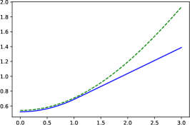
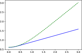
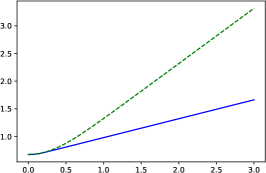
Figure 1. $g_{pl}(\beta,h)$ is in blue (solid), and the RHS of (16) is in green (dotted), each as a function of $h=te_{1}$ From left to right, $\beta$ takes the values $1,3,\textrm{ and }5$.

In these simulations, we can see a high temperature regime for $h$ near $0$ where $g_{pl}(\beta,h)$ coincides with the annealed bound. Then, the free energy smoothly transitions from the high-temperature regime to the low-temperature regime as $g_{pl}(\beta,h)$ becomes strictly smaller than the annealed bound. While the $\beta=3$ and $\beta=5$ graphs appear similar, it seems clear that the phase transition happens at smaller $h$ for larger $\beta$. Our next result indicates why this is true.

Theorem 2.6.

If $(h,\beta_{0})$ is in low temperature, then $(h\beta_{0}/\beta,\beta)$ is also in low temperature for every $\beta>\beta_{0}$.

A similar statement applies with strong disorder replacing low temperature. This result is an adaptation of the classical monotonicity result for $F(\beta)-\mathbb{\Lambda}(\beta)$ [14] to our setting. It requires a little bookkeeping, and its proof can be found in Section 6.

One of the main consequences of the weak-strong disorder phase transition is that the Gibbs measure on the endpoint on the path changes from Gaussian to localized behavior. We present our generalization of these classical results next:

1. a CLT in the $L^{2}$ region of $\operatorname{WEAK}_{\beta}$; i.e., in the set $\{h\colon\mathbb{M}_{2}(\beta)<\pi(q(h))^{-1}\}$, and

2. localization of the endpoint for $h\in\operatorname{STRONG}_{\beta}$.

For both of these results, our proofs primarily involve generalizing classical techniques to general underlying walks $p$. The classical CLT for the polymer endpoint under the Gibbs measure is originally due to Bolthausen [5] when the weights are $\operatorname{Bernoulli}(1/2)$. This was subsequently improved by [12, eq. (2.5) ] using the version of the second moment computation for general weights by [34]. Our generalization of these results involves an additional sub-Gaussianity assumption on $p$. It is of some interest to weaken this condition.

For any positive-definite matrix $\Sigma$, we write $\gamma_{\Sigma}$ for the Gaussian measure with density

$$\gamma_{\Sigma}(x):=\frac{1}{(2\pi)^{d/2}(\det\Sigma)^{1/2}}\exp\left(-\frac{1}{2}x\cdot\Sigma^{-1}x\right),$$ (22)

where $x\cdot y$ is the usual dot product on $\mathbb{R}^{d}$.

Theorem 2.7.

Let $p$ be a random walk kernel whose step distribution is sub-Gaussian; i.e., $\exists C>0$ s.t.

$$\mathbb{E}[e^{t\cdot|X_{1}|}]\leq\exp\left(C|t|^{2}/2\right),$$ (23)

If $\mathbb{M}_{2}(\beta)<\pi(q(h))^{-1}$, $\forall f\in C(\mathbb{R}^{d})$ with at most polynomial growth at $\pm\infty$, we have

$$\lim_{n\to\infty}\bigg{\langle}f\left(\frac{X_{n}-nm_{q(h)}}{\sqrt{n}}\right)\bigg{\rangle}_{n,\beta,q(h)}=\int f\left(x\right)d\gamma_{\Sigma(q(h))}(x)\quad\mathbb{P}-\textrm{a.s}$$ (24)

where $m_{q(h)}=E_{q(h)}[X_{1}]$, and $\Sigma_{q(h)}$ is the covariance matrix of one step of the random walk given by

$$\Sigma_{q(h)}(i,j)=E_{q(h)}\left[\left((X_{1}-m_{q(h)})\cdot e_{i}\right)\left((X_{1}-m_{q(h)})\cdot e_{j}\right)\right].$$

Remark 2.8.

Choosing $f(x)=x$, we see that $\lim_{n\to\infty}\big{\langle}\frac{X_{n}}{n}\big{\rangle}_{n,\beta,q(h)}=E_{q(h)}[X_{1}]~{}\textrm{a.s}$. That is, the endpoint of the polymer is aligned with the drift of the underlying random walk induced by the field. If $p$ has finite range, Theorem 2.3 shows that a low temperature regime exists. This means that the polymer endpoint will be misaligned with the underlying random walk on a nontrivial subset of $h$ in the low temperature regime.

Choosing $f(x)=|x|^{2}$ shows the almost sure diffusive scaling of the endpoint location under the polymer measure.

Remark 2.9.

While we have proved a simple CLT for the endpoint in the $L^{2}$ region of $\operatorname{WEAK}_{\beta}$, it seems clear that one ought to be able to prove a Brownian invariance principle for the entire polymer path in weak disorder, à la [14].

Recall the definition of localization in (10). It follows from the proofs of Theorems 5.1 and 5.4 in [10], that

Theorem 2.10.

If $h\in\operatorname{STRONG}_{\beta}$, then the polymer endpoint is localized.

In this paper, we have merely just begun to scratch the surface of the full phase diagram of the polymer model. We highlight a couple of interesting questions:

1. Can one prove that there is no re-entrant phase transition in $h$, as Figure 1 suggests? The classical FKG proof of monotonicity in $\beta$ for $F(\beta)-\mathbb{\Lambda}(\beta)$ in [14] does not appear to work.

2. Can one define and describe the boundary between $\operatorname{WEAK}_{\beta}$ and $\operatorname{STRONG}_{\beta}$?

2.1. Acknowledgements

The authors would like to thank H. Lacoin for a valuable discussion, and F. Rassoul-Agha, T. Seppäläinen and A. Yilmaz for comments on a first draft. This research was supported in part through computational resources and services provided by Advanced Research Computing at the University of Michigan, Ann Arbor and by the Center for Integrated Research Computing at the University of Rochester.

3. Existence of the free-energy

In this section, we prove Proposition 2.1. When $p$ is finite-range, there is a “point-to-point” analog in [31, Theorem 2.2]; this and the duality relationship (13) imply Proposition 2.1. We establish the analogous theorem for the point-to-level free energy simultaneously for all temperatures $\beta\in(0,\infty)$ and external fields $h\in\mathbb{R}^{d}$.

Proof.

For each $(\beta,h)\in(0,\infty)\times\mathbb{Q}^{d}$, the existence of the limit follows directly from the proofs of Proposition 2.5 and Lemma 3.1 in [9], both of which go through without modification assuming (18). Let

$$g_{n}(\beta,h)=\frac{\log E_{p}\left[\exp\left(\beta(H(\vec{X}_{n})+h\cdot X_{n})\right)|X_{0}=0\right]}{\beta n}.$$

We assume in the following that $X_{0}=0$ to avoid repeating the conditioning in the expectation. Then, it is easy to check that

$$\nabla_{h}g_{n}(\beta,h) =n^{-1}\frac{E_{p}\left[X_{n}\exp\left(\beta(H(\vec{X}_{n})+h\cdot X_{n})\right)\right]}{E_{p}\left[\exp\left(\beta(H(\vec{X}_{n})+h\cdot X_{n})\right)\right]}$$ (25)

$$=n^{-1}\langle X_{n}\rangle_{n,\beta,q(h)}.$$

Similarly, $\partial_{\beta}g_{n}(\beta,h)=n^{-1}\langle H(\vec{X}_{n})+h\cdot X_{n}\rangle_{n,\beta,q(h)}$.

Claim 3.1.

For any fixed $K>0,0<\beta_{1}<\beta_{2}$ and for all $|h|\leq K,\beta\in[\beta_{1},\beta_{2}]$, there is a constant $C$ such that eventually $\mathbb{P}$-almost-surely

1. $|\nabla_{h}g_{n}(\beta,h)|\leq C$, and

2. $|\partial_{\beta}g_{n}(\beta,h)|\leq C$.

Note that we can write $\partial_{\beta}g_{n}(\beta,h)=n^{-1}\langle H(\vec{X}_{n})\rangle_{n,\beta,q(h)}+h\cdot\nabla_{h}g_{n}(\beta,h)$, so proving the Claim is equivalent to proving item 1 and

1. $|n^{-1}\langle H(\vec{X}_{n})\rangle_{n,\beta,q(h)}|\leq C$.

Claim 3.1 shows that $g_{n}$ is eventually uniformly Lipschitz on $\{(\beta,h)\colon|h|\leq K,\beta_{1}\leq\beta\leq\beta_{2}\}$. Since $K,\beta_{1}$ and $\beta_{2}$ are arbitrary and $g_{n}(\beta,h)$ converges on $(\mathbb{Q}\cap(0,\infty))\times\mathbb{Q}^{d}$, the Arzela-Ascoli theorem shows that $g_{n}(\beta,h)$ converges to a $g_{pl}(\beta,h)$ that is continuous on $(0,\infty)\times\mathbb{R}^{d}$.

Taking the second partial derivatives with respect to $h$, we see that

$$\beta^{-1}n\partial_{h_{i}}\partial_{h_{j}}g_{n}(\beta,h)=\langle X_{n}\cdot e_{i}X_{n}\cdot e_{j}\rangle_{n,\beta,q(h)}-\langle X_{n}\cdot e_{i}\rangle_{n,\beta,q(h)}\langle X_{n}\cdot e_{j}\rangle_{n,\beta,q(h)},$$

which is a covariance, and thus the Hessian is positive definite. Therefore, $g_{n}(\beta,h)$ is convex in $h$, and thus, so is $g_{pl}(\beta,h)$. Similarly, the second partial derivative of $g_{n}(\beta,h)$ with respect to $\beta$ is the variance of $H(\vec{X}_{n})+h\cdot X_{n}$, and hence $g_{n}(\beta,h)$ and $g_{pl}(\beta,h)$ are convex in $\beta$ as well. The Hessian of $g_{n}(\beta,h/\beta)$ is again a covariance matrix, which implies the joint convexity of $g_{pl}(\beta,h/\beta)$ in $(\beta,h)$.

We first prove item 1 of the claim. When $p$ is finite-range, this is obvious; in the general case, we will use the fact that both $\mathbb{M}(s)$ and $M_{p}(t)$ are finite on their respective domains, and thus, good large deviations estimates are available.

Let the numerator and denominator of the fraction in (25) be $\operatorname{NUM}$ and $\operatorname{DENOM}$ respectively. To prove item 1 we bound the $\operatorname{NUM}$ from above and $\operatorname{DENOM}$ from below on an event with high probability. Let

$$\operatorname{END}(C_{0})=\{y\in\mathbb{Z}^{d}\colon|y-nE_{p}[X_{1}]|\leq C_{0}n\}.$$

We split up the expectation in the numerator into two terms,

$$\operatorname{\operatorname{NUM}} =E_{p}\left[X_{n}\exp\left(\beta(H(\vec{X}_{n})+h\cdot X_{n})\right)(1_{\operatorname{END}(C_{0})}+1_{\operatorname{END}(C_{0})^{c}})\right]$$ (26)

and note that the second term is the one we must control since $X_{n}$ is well-behaved in the first. Call this term $T_{2}$. We have

$$|T_{2}| \leq E_{p}\left[|X_{n}|\exp\left(\beta(H(\vec{X}_{n})+h\cdot X_{n})\right)1_{\operatorname{END}(C_{0})^{c}}\right]$$

$$\leq E_{p}\left[\exp\left(\beta H(\vec{X}_{n})+(\beta_{2}K+1)|X_{n}|\right)1_{\operatorname{END}(C_{0})^{c}}\right]$$

$$=:\hat{T}_{2}$$

where we have used Hölder to bound the $h\cdot X_{n}$ term, the condition $|h|\leq K$, and the inequality $x<e^{x}$ to absorb the term $|X_{n}|$ into the exponential. Now $\hat{T}_{2}$ is independent of $h$ and much easier to control. Taking expectation, we get

$$\mathbb{E}\left[\sup_{\beta\in[\beta_{1},\beta_{2}]}\hat{T}_{2}\right] =E_{p}\left[\mathbb{E}\left[\sup_{\beta\in[\beta_{1},\beta_{2}]}\exp(\beta H(\vec{X}_{n}))\right]\exp\left((\beta_{2}K+1)|X_{n}|\right)1_{\operatorname{END}(C_{0})^{c}}\right].$$

Splitting the inner expectation into the events $H(\vec{X}_{n})>0$ and $H(\vec{X}_{n}<0)$, we get

$$\mathbb{E}\left[\sup_{\beta\in[\beta_{1},\beta_{2}]}\exp(\beta H(\vec{X}_{n}))\right]\leq(\mathbb{M}(\beta_{1})+\mathbb{M}(\beta_{2}))^{n}.$$

Taking this term out, and using the Cauchy-Schwartz inequality for the remaining $E_{p}$-expectation, we obtain

$$\mathbb{E}\left[\sup_{\beta\in[\beta_{1},\beta_{2}]}\hat{T}_{2}\right] \leq(\mathbb{M}(\beta_{1})+\mathbb{M}(\beta_{2}))^{n}\overline{M}_{p}(d(\beta_{2}K+1))^{n/2}P_{p}(\operatorname{END}(C_{0})^{c})^{1/2}.$$ (27)

In the previous line, $\overline{M}_{p}$ is given by

$$E_{p}[\exp(C|X_{1}|)] \leq E_{p}[\exp(C|X_{1}|_{1})],$$

$$\leq\prod_{j=1}^{d}E_{p}\left[\exp(Cd|X_{1}\cdot e_{j}|)\right]^{1/d},$$

$$\leq\max_{i=1,\ldots,d}(M_{p}(Cde_{i})+M_{p}(-Cde_{i}))$$

$$:=\overline{M}_{p}(Cd),$$

where $|\cdot|_{1}$ is the $\ell^{1}$ norm. Since $M_{p}(t)<\infty$ is finite for all $t$, $X_{n}$ has a good rate function, and $P_{p}(\operatorname{END}(C_{0})^{c})\leq\exp(-nI(C_{0}))$ where $I(C_{0})>0$ for all $C_{0}>0$ and $I(C_{0})\to\infty$ as $C_{0}\to\infty$ (see Cramér’s theorem [28]). Since $K$, $\beta_{1}$ and $\beta_{2}$ are fixed, the right-hand side of (3) can be bounded by $\exp(-C_{1}n)$ where $C_{1}$ can be chosen to be arbitrarily large by choosing $C_{0}$ to be large. Using Chebyshev’s inequality we obtain,

$$\mathbb{P}(|\hat{T}_{2}|>\exp(-C_{1}n/2))\leq\exp(-C_{1}n/2).$$ (28)

Next, we need a lower bound for the denominator in (25). It will be enough for our purposes to bound it by some exponentially decaying function in $n$, as long as the rate is not too small.

As long as $E_{p}[p(X_{1})^{t}]$ is finite in some interval around the origin, Cramér’s theorem again gives us a good rate function $I_{1}$ such that

$$\log\frac{1}{n}P_{p}\left(\bigg{|}\sum_{i=1}\log p(X_{i}-X_{i-1})-E_{p}[\log p(X_{1})]\bigg{|}\geq nt\right)\to-I_{1}(t).$$

$E_{p}[p(X_{1})^{t}]$ can be shown to be finite for $t\in(-1,1)$ as follows: Since $M_{p}$ is finite on its domain, Chebyshev’s inequality gives $P_{p}(|X_{1}|\geq s)\leq\exp(-C_{1}s)E_{p}[\exp(C|X_{1}|)]$. Then,

$$E_{p}[p(X_{1})^{t}]=\sum_{x\in\mathbb{Z}^{d}}p(x)^{1+t}\leq\sum_{k=0}^{\infty}C_{2}k^{d-1}e^{-C_{1}(1+t)k}<\infty.$$

Thus, there is a set $Y_{1}$ of random walk paths such that $P_{p}(Y_{1}^{c})\leq\exp(-nI_{1}(t)/2)$ and

$$\exp(n(E_{p}[\log p(X_{1})]-t))\leq p(\vec{X}_{n})\leq\exp(n(E_{p}[\log p(X_{1})]+t))\quad\forall\vec{X}_{n}\in Y_{1}.$$

Choosing $t=-E_{p}[\log p(X_{1})]/2$, it follows that $|Y_{1}|\leq\exp(n(-3E_{p}[\log p(X_{1})]/2))$.

We can control the weight on the exponentially many paths in $Y_{1}$ using large deviation bounds. Since $\mathbb{M}(\beta)<\infty$, there exists a good rate function $I_{2}$ for iid sums of weights. So, for any $C>0$, there exists $c>0$ such that

$$\mathbb{P}\left(\bigcup_{\vec{X}_{n}\in Y_{1}}|H(\vec{X}_{n})-n\mathbb{E}[\omega_{0}]|>cn\right)\leq|Y_{1}|\exp(-nC).$$ (29)

By choosing $c$ to be large enough, we can get $C>-E_{p}[\log p(X_{1})]+t$, and thus the probability of the event in (29) decays exponentially in $n$.

Since $\operatorname{DENOM}$ is the $P_{p}$-expectation of a positive random variable, we can restrict to a smaller set of paths $Y_{1}\cap\operatorname{END}(C_{2})$. On the complement of the event in (29) we obtain

$$\operatorname{DENOM} =E_{p}\left[\exp(\beta H(\vec{X}_{n})+\beta X_{n}\cdot h)\right]$$

$$\geq E_{p}\left(\exp(n\beta(\mathbb{E}[\omega_{0}]-c))\exp(-n\beta K(C_{2}+|E_{p}[X_{1}]|))1_{Y_{1}\cap\operatorname{END}(C_{2})}\right)$$

$$\geq\frac{1}{2}\exp(n\beta(\mathbb{E}[\omega_{0}]-c-K(C_{2}+|E_{p}[X_{1}]|)),$$

where we have again used the Hölder inequality to control $h\cdot X_{n}$ for $X_{n}\in\operatorname{END}(C_{2})$, and $P_{p}(Y_{1}\cap\operatorname{END}(C_{2}))\geq\frac{1}{2}$, which holds since both $Y_{1}$ and $\operatorname{END}(C_{2})$ have complements with exponentially small probabilities. Note that here $C_{2}$ is an arbitrary positive constant and $c>0$ depends on the constant $C$ in (29), so there exists a constant $C_{3}>0$, independent of $C_{0}$ and $C_{1}$, such that with probability close to $1$, we have

$$\operatorname{DENOM} \geq\exp(-n\beta C_{3}).$$ (30)

Combining (28) and (30), on the complement of the union of the events in (28) and (29) we obtain

$$\left|\frac{\operatorname{NUM}}{\operatorname{DENOM}}\right| \leq(C_{0}+|E_{p}[X_{1}]|)n+\frac{|\hat{T}_{2}|}{\operatorname{DENOM}}$$

$$\leq(C_{0}+|E_{p}[X_{1}]|)n+\exp(-(C_{1}/2-\beta C_{3})n).$$

Dividing by $n$ and using the Borel-Cantelli lemma, we get $|\nabla_{h}g_{n}(\beta,h)|\leq 2C_{0}$ eventually almost-surely.

The proof of item (3) of the claim is similar. The lower bound for the denominator is identical. As in (26), we write the numerator of $\langle H(\vec{X}_{n})\rangle_{n,\beta,q(h)}$ as

$$E_{p}\left[H(\vec{X}_{n})\exp\left(\beta(H(\vec{X}_{n})+h\cdot X_{n})\right)1_{Y_{1}}\right]\\ +E_{p}\left[H(\vec{X}_{n})\exp\left(\beta(H(\vec{X}_{n})+h\cdot X_{n})\right)1_{Y_{1}^{c}}\right].$$ (31)

Using the inequality $|H(\vec{X}_{n})|\leq e^{H(\vec{X}_{n})}$ and $|h|\leq K$, the second term in (31) can be bounded from above by

$$\hat{T}_{3}=E_{p}\left[\exp\left((\beta+1)H(\vec{X}_{n})+\beta_{2}K|X_{n}|\right)1_{Y_{1}^{c}}\right].$$

As in (3) we obtain

$$\mathbb{E}\left[\sup_{\beta\in[\beta_{1},\beta_{2}]}\hat{T}_{3}\right] \leq(\mathbb{M}(\beta_{1}+1)+\mathbb{M}(\beta_{2}+1))^{n}\overline{M}_{p}(d\beta_{2}K)^{n/2}P_{p}(Y_{1}^{c})^{1/2},$$

which is exponentially small in $n$ if the parameter $t$ in the definition of $Y_{1}$ is large enough. Again, as in (28), Chebyshev’s inequality implies that $|\hat{T}_{3}|$ is exponentially small with probability exponentially close to $1$.

To bound the first term in (31) with high probability, note that on the complement of the event in (29), for all $\vec{X}_{n}\in Y_{1}$ we have $|H(\vec{X}_{n})|\leq(c+|\mathbb{E}[\omega_{0}]|)n$ which implies that the first term in (31) is bounded by $(c+|\mathbb{E}[\omega_{0}]|)n\operatorname{DENOM}$. Combining the bounds for both terms in (31) gives the necessary bound for the numerator in item (3).

This completes the proof of the claim and the proposition, establishing existence and convexity of $g_{pl}(\beta,h)$. ∎

4. Weak disorder

Definition 4.1.

We call the random walk with kernel $p$ truly $d$-dimensional if the sublattice of $\mathbb{Z}^{d}$ obtained by the integer span of the support of the random walk is in fact $d$-dimensional. That is, there is an invertible matrix $A$ with coefficients in $\mathbb{Z}$ such that $\operatorname{supp}(p)=A\mathbb{Z}^{d}$.

We will use the following generalization of the standard local central-limit theorem.

Theorem 4.2 (c.f. Theorem 3.3.3[15]).

Let $p$ be truly $d$-dimensional and take values in the sublattice $A\mathbb{Z}^{d}$. Let $m_{p}=E_{p}[X_{1}]$ and $\Sigma$ be the covariance matrix of one step of the random walk under $p$. Then

$$\lim_{n\to\infty}\sup_{x\in A\mathbb{Z}^{d}}n^{d/2}\left|P(S_{n}=x)-\frac{\det(\Sigma^{-1/2}A)}{(2\pi n)^{d/2}}\exp\left(-\frac{\left((x-m_{p}n),\Sigma(x-m_{p}n)\right)}{2n}\right)\right|=0.$$

Theorem 4.3.

Suppose $d\geq 3$, and $\beta>0$. Assume that the condition for weak disorder in (7) is satisfied, and that $p$ is truly $d$-dimensional. Then, there is a $C_{0}>0$ such that for all $\left|{h}\right|<C_{0}$, we have $\mathbb{M}_{2}(\beta)<1/\pi(q(h))$, where $q(h)$ is defined in (14); i.e., the polymer is in the weak disorder regime under the external field $h$.

Proof of Theorem 4.3.

Since the left-hand side of the inequality $\mathbb{M}_{2}(\beta)<1/\pi(q(h))$ is independent of $h$, and we are assuming that the inequality (7) holds when $h=\mathbf{0}$, it is enough to show that $\pi(q(h))$ is continuous (in $h$) at $h=\mathbf{0}$. Recall that we have

$$\pi(q(h))= P_{q(h)}(S_{n}=S_{n}^{\prime}\text{ for some }n>0),$$

which can be interpreted to be the return probability of the origin of the random walk $T_{n}=S_{n}-S_{n}^{\prime}$, where $S_{n}$ and $S_{n}^{\prime}$ are two independent copies of the same random walk. Using the Markov property for this random walk, we have

$$R(q(h)) :=\sum_{n=1}^{\infty}P_{q(h)}(T_{n}=\mathbf{0})=E_{q(h)}[\text{\# of returns of }T_{n}]$$

$$=\sum_{k=1}^{\infty}k\pi^{k}(q(h))(1-\pi(q(h)))=\frac{\pi(q(h))}{1-\pi(q(h))},$$ (32)

where the RHS is to be interpreted as $\infty$ if $\pi(q(h))=1$. In $d\geq 3$, since $\pi(q(\mathbf{0}))<1$, the continuity of $\pi(q(h))$ at $h=\mathbf{0}$ is equivalent to the continuity of $R(q(h))$ at $h=\mathbf{0}$. Later on in the proof, we show that the tails of the sum defining $R(q(h))$ in (32) decay uniformly for $|h|$ small enough; i.e., given $\varepsilon>0$, there exists $C_{1}>0$ and $n_{\varepsilon}$ such that for all $|h|<C_{1}$ and $n>n_{\varepsilon}$, we have $\sum_{n>n_{\varepsilon}}P_{q(h)}(T_{n}=\bar{x})<\varepsilon/3$. Thus,

$$|R(q(h))-R(q(\mathbf{0}))| =\left|\sum_{n}P_{q(h)}(T_{n}=\mathbf{0})-P_{q(\mathbf{0})}(T_{n}=\mathbf{0})\right|$$

$$<2\varepsilon/3+\left|\sum_{n<n_{\varepsilon}}P_{q(h)}(T_{n}=\mathbf{0})-P_{q(\mathbf{0})}(T_{n}=\mathbf{0})\right|.$$ (33)

From (14) and the consequent continuity of the characteristic function $E_{q(h)}[e^{iuT_{n}}]$, it follows that $P_{q(h)}(T_{n}=\mathbf{0})$ is continuous in $h$, and thus, the sum in (33) converges to zero when $h\to\mathbf{0}$. So $\exists C_{2}>0$ such that $\forall|h|<C_{2}$, we have $|\sum_{n<n_{\varepsilon}}P_{q(h)}(T_{n}=\mathbf{0})-P_{q(\mathbf{0})}(T_{n}=\mathbf{0})|<\varepsilon/3$. Setting $C_{0}=\min(C_{1},C_{2})$ we obtain the desired continuity of $R(q(h))$.

Next, we establish the uniform in $h$ bound on the tail of the sum in (32), by using ideas from the proof of the local limit theorem (see e.g. [15]). Consider the $\mathbb{Z}$-span of the support of the random walk $T_{1}$. By assumption, it forms a sublattice of $\mathbb{Z}^{d}$ which has dimension $d$. It follows that there exists an invertible matrix $A$ with coefficients in $\mathbb{Z}$ such that the sublattice in question is equal to $A\mathbb{Z}^{d}$. Note that different choices of bases for the sub-lattice correspond to different matrices $A$, but this will not play a major role in the proof.

We have the identity

$$1_{\{T_{1}=\bar{x}\}}=1_{\{A^{-1}T_{1}=A^{-1}\bar{x}\}}=\frac{1}{(2\pi)^{d}}\int_{-\pi}^{\pi}\cdots\int_{-\pi}^{\pi}e^{iA^{-1}T_{1}\cdot u}e^{-iA^{-1}x\cdot u}du.$$

Taking expectation, we get

$$P_{q(h)}(T_{1}=\bar{x})=\frac{1}{(2\pi)^{d}}\int_{-\pi}^{\pi}\dots\int_{-\pi}^{\pi}\phi_{q(h)}(u)e^{-iA^{-1}\bar{x}\cdot u}du,$$

where $\phi_{q(h)}$ is the characteristic function of $A^{-1}T_{1}$. More generally, for the $n$^th step of the random walk, after a change of coordinates, we can write

$$P_{q(h)}(T_{n}=\bar{x})=\frac{1}{n^{d/2}}\frac{1}{(2\pi)^{d}}\int_{-\pi n^{1/2}}^{\pi n^{1/2}}\dots\int_{-\pi n^{1/2}}^{\pi n^{1/2}}\phi_{q(h)}^{n}(u/\sqrt{n})e^{-i\frac{A^{-1}\bar{x}\cdot u}{\sqrt{n}}}du,$$ (34)

giving us

$$R(q(h))=\sum_{n=1}^{\infty}\frac{1}{n^{d/2}}\frac{1}{(2\pi)^{d}}\int_{-\pi n^{1/2}}^{\pi n^{1/2}}\dots\int_{-\pi n^{1/2}}^{\pi n^{1/2}}\phi_{q(h)}^{n}(u/\sqrt{n})du.$$

Since $\phi_{q(h)}$ is a characteristic function, we have $|\phi_{q(h)}(u)|\leq 1$ for all $u\in\mathbb{R}^{d}$. However, in the region $0<|u_{i}|\leq\pi$, we must have the strict inequality $|\phi_{q(h)}(u)|<1$. If not, for some $u$ in this region, we would have $|\phi_{q(h)}(u)|=1$. This implies that $e^{iA^{-1}T_{1}\cdot u}$ is almost surely constant, so $A^{-1}T_{1}\cdot u\in c+2\pi\mathbb{Z}$ for all possible values of $T_{1}$ for some constant $c$. Since $T_{1}=S_{1}-S_{1}^{\prime}$, we have that $\mathbf{0}$ is in the support of $T_{1}$, and so, without loss of generality $c=0$, giving $A^{-1}T_{1}\cdot u\in 2\pi\mathbb{Z}$. Since the right-hand side is a lattice, we get the same containment by replacing $T_{1}$ by the $\mathbb{Z}$-span of its support, namely $A\mathbb{Z}^{d}$, giving us $A^{-1}A\mathbb{Z}^{d}\cdot u=\mathbb{Z}^{d}\cdot u\in 2\pi\mathbb{Z}$. This is impossible for any $u$ such that $0<|u_{i}|\leq\pi$. Thus, for any $\delta>0$, using continuity of $\phi_{q(h)}(u)$ in $h$ and $u$, there exists a constant $c\in(0,1)$ such that in the region $|h|\leq C_{1}$ and $\delta<\max_{i}|u_{i}|\leq\pi$, we have $|\phi_{q(h)}(u)|\leq c$.

Then, we can estimate the integral in (34) as follows:

$$\left|\int_{[-\pi n^{1/2},\pi n^{1/2}]^{d}}\phi_{q(h)}^{n}(u/\sqrt{n})du\right|$$

$$\quad\leq\int_{[-\delta n^{1/2},\delta n^{1/2}]^{d}}\left|\phi_{q(h)}^{n}(u/\sqrt{n})\right|du+\int_{[-\pi n^{1/2},\pi n^{1/2}]^{d}\backslash[-\delta n^{1/2},\delta n^{1/2}]^{d}}\left|\phi_{q(h)}^{n}(u/\sqrt{n})\right|du$$

$$\quad\leq\int_{[-\delta n^{1/2},\delta n^{1/2}]^{d}}\left|\phi_{q(h)}^{n}(u/\sqrt{n})\right|du+c^{n}(2\pi)^{d}n^{d/2}.$$

Using [15, 3.3.3], we can write

$$|\phi_{q(h)}(u)|\leq 1-\frac{1}{2}E_{q(h)}|u\cdot T_{1}|^{2}+E_{q(h)}\min(|u\cdot T_{1}|^{3},2|u\cdot T_{1}|^{2}).$$

If $u$ is sufficiently close to the origin, the minimum in the last expectation is taken by the cubic term, and we get

$$|\phi_{q(h)}(u)|\leq 1-\frac{1}{4}E_{q(h)}|u\cdot T_{1}|^{2}\leq e^{-\frac{1}{4}E_{q(h)}|u\cdot T_{1}|^{2}},$$

which implies

$$|\phi_{q(h)}(u/\sqrt{n})^{n}|\leq e^{-\frac{1}{4}E_{q(h)}|u\cdot T_{1}|^{2}}\leq e^{-C|u|^{2}}$$

since $q(h)$ is a continuous function of $h$, and $|h|<C_{1}$. Thus, the tail $n\geq m$ of the series for $R(q(h))$ can be estimated from above by

$$\sum_{n=m}^{\infty}\frac{1}{n^{d/2}}\frac{1}{(2\pi)^{d}}\left(\int_{[-\delta n^{1/2},\delta n^{1/2}]^{d}}e^{-C|u|^{2}}du+c^{n}(2\pi)^{d}n^{d/2}\right),$$

which, if $m$ is large enough, is arbitrarily small uniformly in $h$, as needed. notesBasically we use

$$E_{p}[e^{\beta h\cdot(X_{1}+X_{1}^{\prime})}(u\cdot(X_{1}-X_{1}^{\prime}))^{2}]$$

is a continuous function in $h$. ∎

4.1. Endpoint behavior in weak disorder

In this section, we sketch the proof of Theorem 2.7. It follows the presentation in [10, Theorem 3.4 ] to a T, and so we will merely indicate where changes need to be made for a general underlying walk $p$. The best strategy to read this sketch is to read the version in [10] first, and then return here to understand the changes. The only place where the transition probability $p$ matters is in the proof of Prop. 4.4 below.

Without loss of generality, we will assume that $m=E_{p}[X_{1}]=0$ since we can always subtract the mean from the random walk and shift the lattice appropriately. Let $\phi_{k}(n,x)$ be a polynomial in $n$ and $x$ such that $\phi_{k}(n,X_{n})$ is a martingale for the random walk filtration $F_{n}=\sigma(X_{0},\ldots,X_{n})$ satisfying the growth condition

$$\phi_{k}(n,x)\leq C_{0}+C_{1}|x|^{k}+C_{2}n^{k/2}\quad\forall n,x\in\mathbb{Z}_{\geq 0}\times\mathbb{Z}^{d}.$$ (35)

Proposition 4.4 (Proposition 3.2 in [10] or Proposition 3.2.1 in [12]).

Suppose $d\geq 3$, and $\phi_{k}(n,X_{n})$ is a polynomial martingale for the filtration $F_{n}$. Then,

$$M_{n}:=E\left[\phi_{k}(n,X_{n})\exp\left(\beta H(\vec{X}_{n})-n\log\mathbb{\Lambda}(\beta)\right)\right]$$

is a martingale for the filtration $\mathcal{F}_{n}$, and satisfies

1. $\exists\gamma\in[0,k/2)$ such that $\max_{0\leq j\leq n}|M_{j}|=O(n^{\gamma})$ almost surely,

2. $\mathbb{E}[M_{n}^{2}]=O(b_{n,k})$, where

   $$b_{n,k}=\begin{cases}1&k<d/2-1\\ \log(n)&k=d/2-1\\ n^{k-d/2+1}&k>d/2-1\end{cases}$$

Proof of Prop. 4.4.

We follow the proof of [12, Proposition 3.2.1], which is the corresponding statement in the case when $p$ is the simple random walk. In that proof the fact that $p$ is the simple random walk is only used to obtain the estimate (3.15) [12, Lemma 3.2.2], which, in our notation, states

$$E_{p}^{\otimes 2}\left[|X_{n}|^{2k}1_{X_{n}=X_{n}^{\prime}}\right]\leq Cn^{k-d/2}.$$ (36)

While (36) is not true for general random walks $p$ with an exponential moment generating function, we show that it holds under the sub-Gaussianity assumption in (23). First, we note that if $p$ is sub-Gaussian, we have the tail estimate $P_{p}(|X_{n}|\geq t)\leq e^{-t^{2}/(2Cn)}$ and the moment bound

$$E_{p}[|X_{n}|^{k}]=k\int_{0}^{\infty}t^{k-1}P_{p}(|X_{n}|\geq t)dt\leq C_{k}n^{k/2}\quad\forall n.$$ (37)

Using this estimate, we obtain

$$E_{p}^{\otimes 2}\left[|X_{n}|^{2k}1_{X_{n}=X_{n}^{\prime}}\right] =\sum_{x\in\mathbb{Z}^{d}}E_{p}\left[|X_{n}|^{2k}1_{X_{n}=x}\right]P_{p}\left[X_{n}^{\prime}=x\right]$$

$$\leq\frac{C}{n^{d/2}}\sum_{x\in\mathbb{Z}^{d}}E_{p}\left[|X_{n}|^{2k}1_{X_{n}=x}\right]$$

$$=\frac{C}{n^{d/2}}E_{p}\left[|X_{n}|^{2k}\right]$$

$$\leq Cn^{k-d/2},$$

where we have used the local limit theorem (Theorem 4.2) and (37). Note that in the above computations, $C$ is a constant that may change from line to line. Using this estimate, the rest of the argument is identical to [12] or [10] and proves Proposition 4.4. ∎

Proof of Theorem 2.7.

Next, we construct families of martingales $\phi_{a}(n,x)$ and $\psi_{a}(n,x)$ indexed by $a\in\mathbb{Z}_{\geq 0}^{d}$ satisfying (35). Let $a=(a_{j})_{j=1}^{d}$, and

$$|a|_{1}=a_{1}+\cdots+a_{d},x^{a}=x_{1}^{a_{1}}\cdots x_{d}^{a_{d}}.$$

We introduce

$$\phi_{a}(n,x)=\left(\frac{\partial}{\partial\theta}\right)^{a}\exp\left(\theta\cdot x-n\rho(\theta)\right)\bigg{|}_{\theta=\mathbf{0}}$$ (38)

where $\rho(\theta)=\Lambda_{p}(\theta)$ is the log moment generating function of $X_{1}-X_{0}$, the first step of the random walk with kernel $p$. The function $\psi_{a}(n,x)$ is the Gaussian version of $\phi_{a}(n,x)$; i.e., $\rho(\theta)$ is replaced by $\hat{\lambda}(\theta):=(\theta,\Sigma\,\theta)/2$ in (38). It is easy to check that $\psi_{a}(n,x)$ is a polynomial martingale that satisfies (35). The rest of the proof of Theorem 2.7 is identical to [10, Theorem 3.4].

notesThis makes some of the statements in [10] clearer, at least for me, but I’m not sure it’s worth including. It is enough to prove Theorem 2.7 for monomial functions $f(x)=x^{a}$. The proof is by induction on $|a|_{1}$. The base case of $|a|_{1}=0$ is, of course, trivial. Fix any $a\neq\mathbf{0}$. By the induction hypothesis, for any $b$ such that $|b|_{1}<|a|_{1}$, we have

$$\langle\left(\frac{X_{n}}{\sqrt{n}}\right)\rangle\to\int x^{b}d\gamma_{\Sigma}(x).$$

Our version of $(3.17)$ in [12] is

$$\int\psi_{a}(1,x)d\gamma_{\Sigma}(x)=0$$ (39)

To see this, let $Z$ be a centered Gaussian random variable with covariance matrix $\Sigma$. Then, $e^{\theta Z-n\hat{\lambda}(\theta)}$ is an analytic function of $\theta$, and we write the Taylor expansion

$$e^{\theta Z-\hat{\lambda}(\theta)}=1+\sum_{a\in\mathbb{Z}_{\geq 0}^{d}}\theta^{a}\psi_{a}(1,Z).$$

Taking expectation and applying Fubini’s theorem, we see that (39) must hold. As in [12] and [5, Lemma 3c], we write

$$\phi_{a}(n,x) :=x^{a}+\hat{\phi}_{a}(n,x)=x^{a}+\sum_{|b|_{1}+2j\leq|a|_{1},j\geq 1}A_{a}(b,j)x^{b}n^{j}$$ (40)

$$\psi_{a}(n,x) :=x^{a}+\hat{\psi}_{a}(n,x)=x^{a}+\sum_{|b|_{1}+2j=|a|_{1},j\geq 1}A_{a}(b,j)x^{b}n^{j}$$ (41)

In (41), only the $|b|_{1}+2j=|a|_{1}$ terms survive since only the second cumulants of the centered Gaussian are nonzero. In such terms, the coefficients $A_{a}(b,j)$ in both $\hat{\psi}_{a}$ and $\hat{\phi}_{a}$ match because the covariances of the underlying random walk $p$ and the covariances of the Gaussian are chosen to be equal. Finally, we notice from (41) that

$$\frac{1}{n^{|a|_{1}/2}}\hat{\psi}_{a}(n,x)=\hat{\psi}_{a}\left(1,\frac{x}{\sqrt{n}}\right).$$ (42)

Then,

$$\bigg{\langle}\left(\frac{X_{n}}{\sqrt{n}}\right)^{a}\bigg{\rangle} =\frac{1}{n^{|a|_{1}/2}}E\left[\left(\phi_{a}\left(n,X_{n}\right)-\hat{\phi}_{a}\left(n,X_{n}\right)+\hat{\psi}_{a}\left(n,X_{n}\right)-\hat{\psi}_{a}\left(n,X_{n}\right)\right)\mu(\vec{X}_{n})\right]$$

$$=\frac{1}{n^{|a|_{1}/2}}E\left[\left(\phi_{a}\left(n,X_{n}\right)-\hat{\phi}_{a}\left(n,X_{n}\right)+\hat{\psi}_{a}\left(n,X_{n}\right)-\hat{\psi}_{a}\left(n,X_{n}\right)\right)\mu(\vec{X}_{n})\right]$$

$$=\frac{1}{W_{n}}\frac{M_{n}}{n^{|a|_{1}/2}}+\frac{1}{n^{|a|_{1}/2}}\bigg{\langle}\left(\hat{\phi}_{a}\left(n,X_{n}\right)-\hat{\psi}_{a}\left(n,X_{n}\right)\right)\bigg{\rangle}$$

$$\hphantom{=}-\bigg{\langle}\hat{\psi}_{a}\left(1,\frac{X_{n}}{\sqrt{n}}\right)\bigg{\rangle}$$

The first term goes to $0$ from item 2 in Proposition 4.4. The second term is a polynomial with order strictly less than $|a|_{1}$. So by the induction assumption, each term in that polynomial converges to the Gaussian integral in (24). Combining this with the observation in (39), we see that

$$\lim_{n\to\infty}-\bigg{\langle}\hat{\psi}_{a}\left(1,\frac{X_{n}}{\sqrt{n}}\right)\bigg{\rangle}=\int x^{a}d\gamma_{\Sigma}(x).$$ (43)

The integrand in the third term consists entirely of terms of the form $x^{b}n^{j}$ where $|b|_{1}+2j<|a|_{1}$. Thus, again applying (24) for powers of lower order than $|a|_{1}$, the third term goes to $0$. This completes the proof of the theorem. ∎

5. Strong disorder

In this section, we first complete the proof of Theorems 2.4 and 2.3. The weak disorder part of Theorem 2.3 (item 1) has been proven in Theorem 4.3. The strong disorder part of Theorem 2.3 requires the entropy condition for strong disorder in Theorem 2.4, which in turn relies on Proposition 5.1, Lemma 44, and Lemma 5.3.

Proposition 5.1 gives a condition for strong disorder that compares a relative entropy of the weights with the Shannon entropy of the underlying random walk. It ought to be interpreted as saying that when the entropy of the weights (impurities) overwhelms the entropy of the underlying random walk (the thermal fluctuations), the polymer is in the strong disorder regime. Then, we prove Lemma 44, which shows that if $p$ has a finite logarithmic moment and the conditions of Theorem 2.4 are satisfied for some field $h$, then the behavior of the Shannon entropy of the random walk with kernel $q(\lambda h)$ as $\lambda\to\infty$ can be understood. Then, in Lemma 5.3, we show that if $p$ has finite range, the favorable $h$ required by Lemma 44 exist, and $H(q(\lambda h))\to 0$ as $\lambda\to\infty$. This shows that there are fields $h$ satisfying the entropy condition in Proposition 5.1, thereby implying high temperature and strong disorder.

Finally, we show that we cannot draw the same conclusions for Gaussian polymers since for all values of the external field $h$, the entropy of the random walk $q(h)$ remains strictly above $0$; i.e., the conclusion of Lemma 5.3 does not hold.

Proposition 5.1.

Suppose $\beta>0$ is such that $H(\mathbb{P}|\mathbb{Q}_{\beta})>H(p)$, where $p$ is a (nontrivial) random walk transition probability. Then, the polymer is in the low temperature (and hence strong disorder) regime.

Lemma 5.2.

Suppose $E_{p}|\log(p(X_{1}))|<\infty$, and there is a nonempty set $K\subset\mathbb{Z}^{d}$ such that $\operatorname{argmax}_{x\in\operatorname{supp}(p)}h\cdot{x}=K\subset\mathbb{Z}^{d}$. Then,

$$\lim_{\lambda\to\infty}H(q(\lambda h))=H_{K}(p).$$ (44)

Lemma 5.3.

Suppose $p$ is nontrivial and has finite range. Then, there exist $h$ such that $K(h)$ is a singleton, and hence $H_{K(h)}=0$.

Using these three ingredients, we complete the proof of Theorem 2.4, and use that to prove Theorem 2.3.

Proof of Theorem 2.4.

Fix $h\in\mathbb{R}^{d}$ such that $K(h)$ is nonempty. Lemma 44 guarantees that $H(q(\lambda h))\to H_{K(h)}(p)$ as $\lambda\to\infty$. Then, choose $\lambda$ so large, such that $H(\mathbb{P}|\mathbb{Q}_{\beta})>H(q(\lambda h))$, and it follows from Proposition 5.1 that the polymer is in the low temperature regime under the external field $\lambda h$. ∎

Proof of Theorem 2.3.

The proof of item 1 is a direct consequence of Theorem 4.3.

Item 2 follows from Lemmas 44 and 5.3. If $p$ is nontrivial and has finite range, then for every $\beta>0$, there exist $h$ such that $K(h)$ is a singleton and hence $H_{K(h)}=0$. It is clear that $K(\lambda h)=K(h)$ for all $\lambda>0$, and since $p$ has finite range, $E_{p}|\log(p(X_{1}))|<\infty$. Since $H(\mathbb{P}|\mathbb{Q}_{\beta})$ is a relative entropy of measures, it is nonnegative. Moreover, it is $0$ if and only if $\mathbb{P}(\omega)$ is a delta mass or if $\beta=0$. Then, it follows from (44) that for large enough $\lambda$, $H(q_{p}(\lambda h))<H(\mathbb{P}|\mathbb{Q}_{\beta})$. Hence, the conditions of Theorem 2.4 are satisfied and $\lambda h\in\operatorname{STRONG}_{\beta}$. ∎

Proof of Proposition 5.1.

We mimic the classical Kahane-Peyriere argument [10] to obtain the entropic condition in (21) that ensures that the polymer is in the low temperature regime; i.e., strict inequality holds in the annealed bound.

Fix $\theta\in(0,1)$ and for this section alone, let us introduce the notation

$$Z_{i,j}(x)=E_{p}\left(\exp(\beta H(\vec{X}_{i,j}))|X_{i}=x\right)$$

where $\vec{X}_{i,j}=(X_{i},\ldots,X_{j})$ refers to the section of the random walk path from step $i$ to $j$. Using $(x+y)^{\theta}\leq x^{\theta}+y^{\theta}$ when $\theta\in(0,1)$, we get

$$Z_{0,n}(\mathbf{0})^{\theta} =\left(\sum_{x}p(x)Z_{1,n}(x)e^{\beta\omega_{1,x}}\right)^{\theta}$$

$$\leq\sum_{x}p(x)^{\theta}Z_{1,n}(x)^{\theta}e^{\theta\beta\omega_{1,x}}.$$

Normalizing the partition function, taking expectation, and using independence, we get

$$\mathbb{E}W_{n}^{\theta}\leq\sum_{x}p(x)^{\theta}\frac{\mathbb{E}[Z_{1,n}(x)^{\theta}]}{\mathbb{M}(\beta)^{(n-1)\theta}}\frac{\mathbb{E}[e^{\theta\beta\omega_{1,x}}]}{\mathbb{M}(\beta)^{\theta}}=r(\theta)\mathbb{E}[W_{n-1}^{\theta}],$$

where

$$r(\theta)=\frac{\mathbb{M}(\theta\beta)}{\mathbb{M}(\beta)^{\theta}}\sum_{x}p(x)^{\theta}.$$ (45)

We will show $r(\theta)<1$ next, from which it will follow that

$$\frac{1}{n}\log\mathbb{E}[W_{n}^{\theta}]\leq\log r(\theta)<0.$$

Then, the Markov inequality and Borel-Cantelli lemma imply the almost sure exponential decay of $W_{n}$ to $0$. notes$\mathbb{P}(W_{n}>n^{-1})\leq\mathbb{E}[W_{n}^{\theta}]n^{\theta}$.

To show $r(\theta)<1$, we first show that the function $\log r(\theta)$ is convex. Since $\log r(\theta)=-\theta\mathbb{\Lambda}(\beta)+\mathbb{\Lambda}(\theta\beta)+\log\sum_{x}p(x)\exp((\theta-1)\log p(x))$, it is a sum of a term linear in $\theta$, and two terms of the form $\log E[\exp(\theta X+Y)]$, where $E$ is either $\mathbb{E}$ or $E_{p}$, and $X$ and $Y$ are the appropriate random variables. Differentiating with respect to $\theta$, we see that

$$\frac{d}{d\theta}\log E[\exp(\theta X+Y)] =\frac{E[X\exp(\theta X+Y)]}{E[\exp(\theta X+Y)]},$$

$$\frac{d^{2}}{d\theta^{2}}\log E[\exp(\theta X+Y)] =\frac{E[X^{2}\exp(\theta X+Y)]}{E[\exp(\theta X+Y)]}-\frac{E[X\exp(\theta X+Y)]^{2}}{E[\exp(\theta X+Y)]^{2}}.$$

Thus the first and second derivatives are the mean and variance of the random variable $X$ with respect to a weighted measure, and this proves that the second derivatives are nonnegative. Note that $\log r(0)=\log\sum_{x}p(x)^{0}=\log(\operatorname{supp}(p))>0$ if the underlying random walk is nontrivial, and that $\log r(1)=0$. Thus, we would only be able to find $\theta$ such that $r(\theta)<1$ if $d\log r(\theta)/d\theta|_{\theta=1}>0$. This gives us the condition

$$\frac{d}{d\theta}\log r(\theta)\big{|}_{\theta=1} =\beta\mathbb{\Lambda}^{\prime}(\theta\beta)-\mathbb{\Lambda}(\beta)+\frac{\sum_{x}p(x)^{\theta}\log p(x)}{\sum_{x}p(x)^{\theta}}\Bigg{|}_{\theta=1}$$

$$=\beta\mathbb{\Lambda}^{\prime}(\beta)-\mathbb{\Lambda}(\beta)-H(p)=H(\mathbb{P}|\mathbb{Q}_{\beta})-H(p)>0,$$

where in the last equality we used (9). In the standard nearest-neighbor random walk case, $H(p)=\log 2d$, and this gives the classical condition for low temperature (see Proposition 1.3). ∎

Proof of Lemma 44.

Let $k=\max_{x\in\operatorname{supp}(p)}h\cdot x$. Then, the dominated convergence theorem gives us that

$$\lim_{\lambda\to\infty}E[e^{\beta\lambda(h\cdot X_{1}-k)}1_{X_{1}\in K^{c}}] =0.$$

The latter can be written more succinctly as $E[e^{\beta\lambda h\cdot X_{1}}]=e^{\beta\lambda k}p(K)(1+o(1))$. Then, as $\lambda\to\infty$,

$$H(q(\lambda h)) =-E\left[\frac{e^{\beta\lambda h\cdot X_{1}}}{E[e^{\beta\lambda h\cdot X_{1}}]}\log\left(p(X_{1})\frac{e^{\beta\lambda h\cdot X_{1}}}{E[e^{\beta\lambda h\cdot X_{1}}]}\right)\right],$$

$$=-E\left[\frac{1}{(p(K)+o(1))}\left(\log\frac{p(X_{1})}{p(K)}+o(1)\right)1_{X_{1}\in K}\right],$$

$$\quad-E\left[\frac{e^{\beta\lambda(h\cdot X_{1}-k)}}{(p(K)+o(1))}\left(\log\frac{p(X_{1})}{p(K)}+o(1)\right)1_{X_{1}\in K^{c}}\right],$$

$$=H_{K}(p)+o(1),$$

where in the last equality we have used the integrability of $|\log p(X_{1})|$ and applied the dominated convergence theorem. ∎

Proof of Lemma 5.3.

Fix $h=(h_{1},h_{2},0,\ldots,0)$ such that $h_{1}/h_{2}$ is a finite irrational. Since $\operatorname{supp}(p)$ has finite cardinality, there must be a unique $x\in\operatorname{supp}(p)$ where $h\cdot x$ takes its maximum. Suppose not; then, there must exist integers $z_{1},z_{2}$ (wlog $z_{2}\neq 0$) such that $\sum_{i=1}^{2}h_{i}z_{i}=0$, or $z_{2}=-(h_{1}/h_{2})z_{1}$. This is a contradiction since $h_{1}/h_{2}$ was assumed to be irrational. Therefore, the cardinality of $K(h)$ is $1$, and consequently $H_{K(h)}(p)=0$. ∎

5.1. Gaussian random walk

Finally, we consider the case where $p$ is a (discrete) Gaussian random walk to illustrate the failure of Lemma 5.3 when $p$ does not have finite range. In dimension $d=1$ consider the random walk where $p(x)=Ce^{-x^{2}/2}$, where the normalization constant $C=\sum_{x}e^{-x^{2}/2}$ is chosen so $p$ is a probability distribution.

Setting $t=\lambda h$, $C_{0}(t)=\sum_{x\in\mathbb{Z}-t}e^{-x^{2}/2}$ and $C_{2}(t)=\sum_{x\in\mathbb{Z}-t}x^{2}e^{-x^{2}/2}$, we have

$$E_{p}(e^{\lambda hx})=C\sum_{x\in\mathbb{Z}}e^{tx-x^{2}/2}=Ce^{t^{2}/2}\sum_{x\in\mathbb{Z}}e^{-(x-t)^{2}/2}=Ce^{t^{2}/2}C_{0}(t).$$

Thus,

$$H(q_{p}(\lambda h))= -\sum_{x}\frac{e^{\lambda hx}}{E(e^{\lambda hx})}p(x)(\ln p(x)+\lambda hx-\ln E(e^{\lambda hx}))$$

$$= \ln C_{0}(t)-\sum_{x}\frac{e^{-(x-t)^{2}/2}}{C_{0}(t)}\left(-\frac{(x-t)^{2}}{2}\right)$$

$$= \ln C_{0}(t)+\frac{C_{2}(t)}{2C_{0}(t)}.$$

Note, that the dependence of $C_{0}$ and $C_{2}$ on $t$ is only in the set over which they are summed. If $t$ ranges over the integers, we have $\mathbb{Z}-t=\mathbb{Z}$, so $C_{0}(t)$ and $C_{2}(t)$ are constants independent of $t$. Both are super-exponentially decaying series, and so can easily be approximated by the first few terms. In fact, both are approximately equal to $2.5$, giving $H(q_{p}(t))\approx 1.4$.

For non-integer $t$’s we can estimate as follows. First, both $C_{0}$ and $C_{1}$ are periodic with period $1$, so for our estimates, without loss of generality, we can assume $0<t<1$. In fact $C_{0}(t)=C_{0}(1-t)$ and $C_{2}(t)=C_{2}(1-t)$, so we can further assume $0<t\leq 1/2$. We have $e^{-(n+t)^{2}/2}\geq e^{-n^{2}/2}$ for $n\leq-1,n\in\mathbb{Z}$ and $e^{-(n+t)^{2}/2}>e^{-(n+1)^{2}/2}$ for $n\geq 2,n\in\mathbb{Z}$, so

$$C_{0}(t)\geq e^{-t^{2}/2}+e^{-(t+1)^{2}/2}-e^{0}-e^{-1/2}-e^{-2^{2}/2}+C_{0}(0).$$

The right-hand side is minimized when $t=1/2$ giving $C_{0}(t)>C_{0}(0)-0.54$. Similarly, we can get $C_{0}(t)<C_{0}(0)+0.51$ giving us $1.96<C_{0}(t)<3.04$. Arguing in the same way we can establish $C_{2}(0)+0.43>C_{2}(t)>C_{2}(0)-0.41$ giving us $2.08<C_{2}(t)<2.93$. Combining these estimates, we get that for any $t$ we have

$$1.01<\ln 1.96+\frac{2.08}{2\cdot 3.04}<H(q_{p}(t))<\ln 3.04+\frac{2.93}{2\cdot 1.96}<1.85.$$

In dimension $d\geq 1$ consider $p(x)=e^{-C|x|^{2}/2}$. Note, that since $p$ is of the form $p(x)=p_{1}(x_{1})\dots p_{d}(x_{d})$, where $p_{1},\dots,p_{d}$ are $d$ copies of the $1$-dimensional discrete Gaussian we considered above, then $H(p)=H(p_{1})+\dots+H(p_{d})=dH(p_{1})$, so for general $d$ we still have that $H(q_{p}(t))$ is independent of $t$ if $t$ is an integer, and for general $t$ we get the bounds

$$1.01d<H(q_{p}(t))<1.85d.$$

It follows that in the case of the discrete Gaussian walk there doesn’t exist $h\in\mathbb{R}^{d}$ such that the entropy of the walk with kernel $q(\lambda h)$ goes to $0$ as $\lambda\to\infty$, and so our theorem cannot guarantee the existence of strong disorder at all $\beta$. notes

6. Monotonicity

In this section we prove Theorem 2.6, which says that if $h\in\operatorname{STRONG}_{\beta_{0}}$, then $h\beta_{0}/\beta\in\operatorname{STRONG}_{\beta}$ for all $\beta>\beta_{0}$. Recall the definition of $g_{pl}(\beta,h)$ in (12) and $\Lambda_{p}(\beta h)$ just below (16). Let

$$\hat{g}_{n}(\beta,h)=\frac{1}{n}\log E_{q(h/\beta)}\left[\exp(\beta H(\vec{X}_{n}))|X_{0}=\mathbf{0}\right]+\Lambda_{p}(h).$$ (46)

Note that $q(h/\beta)$ is actually independent of $\beta$, and the only dependence on $\beta$ in the first term in (46) is in $\beta H(\vec{X}_{n})$. It is clear that $\lim_{n\to\infty}\hat{g}_{n}(\beta,h)=:\hat{g}(\beta,h)=\beta g_{pl}(\beta,h/\beta)$ in $L^{1}$ and $\mathbb{P}-\textrm{a.s}$.

Proposition 6.1.

The function $\beta\mapsto\hat{g}(\beta,h)-\mathbb{\Lambda}(\beta)-\Lambda_{p}(\beta h)$ is nonincreasing on $\mathbb{R}_{\geq 0}$ and nondecreasing on $\mathbb{R}_{\leq 0}$.

The proof of the proposition follows the clever application of the FKG inequality used in [14, Theorem 3.2(b)].

Proof.

We will show that for fixed $h$, $\beta\to\mathbb{E}[\hat{g}_{n}(\beta,h)]-\mathbb{\Lambda}(\beta)-\Lambda_{p}(h)$ is nonincreasing on $\mathbb{R}_{\geq 0}$ and nondecreasing on $\mathbb{R}_{\leq 0}$. Taking $n\to\infty$ produces the result we need. Differentiating with respect to $\beta$, we get

$$\mathbb{E}[\partial_{\beta}\hat{g}_{n}(\beta,h)]=\frac{1}{n}\mathbb{E}\left[\frac{E_{q(h/\beta)}[H(\vec{X}_{n})\exp(\beta H(\vec{X}_{n}))]}{Z_{n,\beta,q(h/\beta)}}\right].$$ (47)

For any fixed random walk path $\vec{X}_{n}$, let the probability measure $\hat{\mathbb{P}}(\{\omega_{x}\}_{x\in\mathbb{Z}^{d}})$ be the measure defined by

$$\int f(\omega)\hat{\mathbb{P}}(d\omega)=\int f(\omega)\exp(\beta H(\vec{X}_{n})-n\mathbb{\Lambda}(\beta))\mathbb{P}(d\omega),$$ (48)

and let $\hat{\mathbb{E}}$ be the corresponding expectation.

It is easy to see that $\hat{\mathbb{P}}$ is a product measure. Note that when $\beta>0$, $H(\vec{X}_{n})$ and $Z_{n,\beta,q(h/\beta)}$ are both increasing functions of the weights $\{\omega_{x}\}_{x\in\mathbb{Z}^{d}}$. Then, using the FKG inequality for the measure $\hat{\mathbb{P}}$ as in [10, pp. 1755], we get

$$E_{q(h/\beta)}\mathbb{E}\Bigg{[} \frac{H(\vec{X}_{n})\exp(\beta H(\vec{X}_{n})-n\mathbb{\Lambda}(\beta))}{Z_{n,\beta,q(h/\beta)}}\Bigg{]}\mathbb{M}(\beta)^{n}=E_{q(h/\beta)}\hat{\mathbb{E}}\left[\frac{H(\vec{X}_{n})}{Z_{n,\beta,q(h/\beta)}}\right]\mathbb{M}(\beta)^{n}$$

$$\leq E_{q(h/\beta)}\bigg{[}\mathbb{E}[H(\vec{X}_{n})\exp(\beta H(\vec{X}_{n})-n\mathbb{\Lambda}(\beta))]$$

$$\qquad\times\mathbb{E}[Z_{n,\beta,q(h/\beta)}^{-1}\exp(\beta H(\vec{X}_{n})-n\mathbb{\Lambda}(\beta))]\bigg{]}\mathbb{M}(\beta)^{n}$$

$$=n\mathbb{\Lambda}^{\prime}(\beta).$$

Plugging this back into (47), we see that

$$\partial_{\beta}(\mathbb{E}[\hat{g}_{n}(\beta,h)]-\mathbb{\Lambda}(\beta)-\Lambda_{p}(h))\leq 0.$$

In the case $\beta<0$, the partition function $Z_{n,\beta,q(h/\beta)}$ is a decreasing function of the weights $\{\omega_{x}\}_{x\in\mathbb{Z}^{d}}$ so the inequalities above are reversed. Taking $n\to\infty$ completes the proof. ∎

Proof of Theorem 2.6.

Suppose $h\in\operatorname{STRONG}_{\beta_{0}}$ for some $\beta_{0}>0$. Then, $\hat{g}(\beta_{0},h\beta_{0})<\mathbb{\Lambda}(\beta_{0})+\Lambda_{p}(h\beta_{0}),$ and it follows from Proposition 6.1 that

$$\hat{g}(\beta,h\beta_{0})<\mathbb{\Lambda}(\beta)+\Lambda_{p}(h\beta_{0})\quad\forall\beta>\beta_{0}.$$ (49)

This implies that $\beta g_{pl}(\beta,\beta_{0}h/\beta)<\mathbb{\Lambda}(\beta)+\Lambda_{p}(\beta_{0}h)$, and thus $\beta_{0}h/\beta\in\operatorname{STRONG}_{\beta}$. ∎

7. Numerical Results

In this section, we present some numerical experimental results in the $d=1$ and $d=3$ cases where the weights are iid $\operatorname{Uniform}[0,1]$ random variables, $p$ is the nearest-neighbor simple random walk, and $\beta=1$ throughout. Figure 1 clearly showed the phase transition in $d=3$ as $g_{pl}(\beta,h)$ diverged away from the annealed bound when $h$ was increased. We were curious to see if the phase transition appeared at the level of fluctuations in numerical simulations. So we simulated the growth exponents for the standard deviation of the log partition function and several other quantities related to the fluctuation of the endpoint. They are

1. $\sqrt{\mathbb{E}[\log(Z_{n})^{2}]-\mathbb{E}[\log(Z_{n})]^{2}}$, the variance of the log partition function.

2. $\mathbb{E}\left[\langle|X_{n}|^{2}\rangle-\langle|X_{n}|\rangle^{2}\right]$, the annealed variance of the endpoint under the Gibbs measure.

3. $\sqrt{\mathbb{E}[A_{n}^{2}]-\mathbb{E}[A_{n}]^{2}}$, where $A_{n}=\operatorname{argmax}_{|z|_{1}=n}\langle 1_{X_{n}=z}\rangle$. This is the standard deviation of the location of the maximum of the Gibbs measure.

4. $\sqrt{\mathbb{E}[\langle|X_{n}|_{2}^{2}\rangle]-\mathbb{E}[\langle|X_{n}|\rangle]^{2}}$, the standard deviation of the endpoint under the annealed Gibbs measure.

We simulated these statistics for four different parameter combinations.

• $d=1,h=0,n=10000,1000$ samples of the environment

• $d=1,h=3,n=10000,1000$ samples of the environment

• $d=3,h=0,n=400,100$ samples of the environment

• $d=3,h=3,n=400,100$ samples of the environment

The simulations for $d=3$ were constrained by memory and runtime. If $t(n)$ is the quantity of interest, we determined the growth exponent by fitting a line to the graph of $\log(t(k))$ versus $\log(k)$ for $k=1,\ldots,n$ and determining the slope. The results appear in Table 1.

Statistic	$d=1$		$d=3$		Exponent
	$h=0$	$h=3$	$h=0$	$h=3$
$\sqrt{\mathbb{E}[\log(Z_{n})^{2}]-\mathbb{E}[\log(Z_{n})]^{2}}$	0.32	0.35	0.03	0.05	$\chi$
$\sqrt{\mathbb{E}\left[\langle|X_{n}|^{2}\rangle-\langle|X_{n}|\rangle^{2}\right]}$	0.51	0.49	0.49	0.51	1/2
$\sqrt{\mathbb{E}[\langle|X_{n}|_{2}^{2}\rangle]-\mathbb{E}[\langle|X_{n}|\rangle]^{2}}$	0.59	0.63	0.49	0.51	$\xi$
$\sqrt{\mathbb{E}[A_{n}^{2}]-\mathbb{E}[A_{n}]^{2}}$	0.65	0.67	0.41	0.46	$\xi$

Table 1. Various endpoint and partition function fluctuation statistics

The variance of the log partition function is thought to grow like $n^{\chi}$, where $\chi$ is called the fluctuation exponent. For the special log-gamma polymer in $d=1$, $\chi$ is known to be $2/3$ [33], but this is expected to be true in much wider generality; this is the KPZ universality conjecture. For $d\geq 3$, when $\beta$ is in the $L^{2}$ portion of the weak-disorder regime, it is clear that the fluctuations are $O(1)$, and thus $\chi=0$. Little is known or conjectured about $\chi$ outside of these regimes.

In the physics literature, [18] conjectured that the annealed variance of the endpoint under the Gibbs measure grows linearly. This was also seen in the numerical experiments in [24]. Our results show that this is indeed the case in $d=1$ and in $d=3$ in both the weak and strong disorder regimes. This is related to the non-zero and bounded curvature of $g_{pl}(\beta,h)$.

In $d=1$, again, physical arguments and numerical simulations suggest that the standard deviation of the argmax of the Gibbs measure grows with transversal fluctuations exponent $\xi=2/3$. Related quantities have been computed for the special log-gamma polymer: Seppäläinen considered the point-to-point polymer, and showed that the transversal fluctuation exponent at intermediate times is bounded above by $2/3$ [33, Theorem 2.5]. Some fluctuation results have also been proved for the half-space log-gamma polymer [2].

In weak disorder in $d\geq 3$, these fluctuations ought to be diffusive and grow with exponent $1/2$ at least when $h=0$, which certainly ought to be in the weak disorder phase. However, our simulated growth exponents are a bit smaller than $1/2$. This is probably because $n$ and the number of samples are both too small, and so these results ought not to be taken seriously.

Given the results of item 3 in $d=1$, if the annealed Gibbs measure on the endpoint assigns an $O(1)$ probability to a region around its maximum, the standard deviation of the endpoint under the annealed Gibbs measure should fluctuate with at least exponent $2/3$. However, our results (especially the one for $d=1,h=0$) suggest that the standard deviation grows with an exponent significantly smaller than $2/3$, which implies that the annealed Gibbs measure on the endpoint concentrates quite sharply around its maximum.

The results for $d=3$ suggest that the standard deviation of the endpoint under the annealed Gibbs measure is diffusive, which is pretty counterintuitive. This again suggests that $n=500$ is probably too low for the purposes of computing the fluctuation exponents in $d=3$.

References

• [1] Sergio Albeverio and Xian Yin Zhou “A martingale approach to directed polymers in a random environment” In J. Theoret. Probab. 9.1, 1996, pp. 171–189 DOI: 10.1007/BF02213739
• [2] Guillaume Barraquand, Ivan Corwin and Sayan Das “KPZ exponents for the half-space log-gamma polymer”, 2023 arXiv:2310.10019 [math.PR]
• [3] Guillaume Barraquand, Ivan Corwin and Evgeni Dimitrov “Fluctuations of the log-gamma polymer free energy with general parameters and slopes” In Probab. Theory Related Fields 181.1-3, 2021, pp. 113–195 DOI: 10.1007/s00440-021-01073-1
• [4] Erik Bates and Sourav Chatterjee “The endpoint distribution of directed polymers” In Ann. Probab. 48.2, 2020, pp. 817–871 DOI: 10.1214/19-AOP1376
• [5] Erwin Bolthausen “A note on the diffusion of directed polymers in a random environment” In Comm. Math. Phys. 123.4, 1989, pp. 529–534 URL: http://projecteuclid.org/euclid.cmp/1104178982
• [6] Alexei Borodin, Ivan Corwin and Daniel Remenik “Log-gamma polymer free energy fluctuations via a Fredholm determinant identity” In Comm. Math. Phys. 324.1, 2013, pp. 215–232 DOI: 10.1007/s00220-013-1750-x
• [7] Philippe Carmona and Yueyun Hu “On the partition function of a directed polymer in a Gaussian random environment” In Probab. Theory Related Fields 124.3, 2002, pp. 431–457 DOI: 10.1007/s004400200213
• [8] Philippe Carmona and Yueyun Hu “Universality in Sherrington-Kirkpatrick’s spin glass model” In Ann. Inst. H. Poincaré Probab. Statist. 42.2, 2006, pp. 215–222 DOI: 10.1016/j.anihpb.2005.04.001
• [9] F. Comets “Weak disorder for low dimensional polymers: the model of stable laws” In Markov Process. Related Fields 13.4, 2007, pp. 681–696
• [10] Francis Comets “Directed polymers in random environments” Lecture notes from the 46th Probability Summer School held in Saint-Flour, 2016 2175, Lecture Notes in Mathematics Springer, Cham, 2017, pp. xv+199 DOI: 10.1007/978-3-319-50487-2
• [11] Francis Comets, Tokuzo Shiga and Nobuo Yoshida “Directed polymers in a random environment: path localization and strong disorder” In Bernoulli 9.4, 2003, pp. 705–723 DOI: 10.3150/bj/1066223275
• [12] Francis Comets, Tokuzo Shiga and Nobuo Yoshida “Probabilistic analysis of directed polymers in a random environment: a review” In Stochastic analysis on large scale interacting systems 39, Adv. Stud. Pure Math. Math. Soc. Japan, Tokyo, 2004, pp. 115–142
• [13] Francis Comets and Vincent Vargas “Majorizing multiplicative cascades for directed polymers in random media” In ALEA Lat. Am. J. Probab. Math. Stat. 2, 2006, pp. 267–277
• [14] Francis Comets and Nobuo Yoshida “Directed polymers in random environment are diffusive at weak disorder” In Ann. Probab. 34.5, 2006, pp. 1746–1770 DOI: 10.1214/009117905000000828
• [15] Rick Durrett “Probability: theory and examples” 31, Cambridge Series in Statistical and Probabilistic Mathematics Cambridge University Press, Cambridge, 2010, pp. x+428 DOI: 10.1017/CBO9780511779398
• [16] Ryoki Fukushima and Stefan Junk “Moment characterization of the weak disorder phase for directed polymers in a class of unbounded environments” In Electronic Communications in Probability, 2023 URL: https://api.semanticscholar.org/CorpusID:257353453
• [17] Nicos Georgiou, Firas Rassoul-Agha and Timo Seppäläinen “Variational formulas and cocycle solutions for directed polymer and percolation models” In Comm. Math. Phys. 346.2, 2016, pp. 741–779 DOI: 10.1007/s00220-016-2613-z
• [18] D.. Huse and C.. Henley “Pinning and roughening of domain walls in Ising systems due to random impurities” In Physical Review Letters 54, 1985, pp. 2708–2711 DOI: 10.1103/PhysRevLett.54.2708
• [19] J.. Imbrie and T. Spencer “Diffusion of directed polymers in a random environment” In J. Statist. Phys. 52.3-4, 1988, pp. 609–626 DOI: 10.1007/BF01019720
• [20] Ernst Ising “Beitrag zur Theorie des Ferromagnetismus” In Zeitschrift für Physik 31.1, 1925, pp. 253–258 DOI: 10.1007/BF02980577
• [21] Stefan Junk “New Characterization of the Weak Disorder Phase of Directed Polymers in Bounded Random Environments” In Communications in Mathematical Physics 389, 2022 DOI: 10.1007/s00220-021-04259-9
• [22] Stefan Junk and Hubert Lacoin “Strong disorder and very strong disorder are equivalent for directed polymers” arXiv:2402.02562 [math-ph] arXiv, 2024 URL: http://arxiv.org/abs/2402.02562
• [23] J.-P. Kahane and J. Peyrière “Sur certaines martingales de Benoit Mandelbrot” In Advances in Math. 22.2, 1976, pp. 131–145 DOI: 10.1016/0001-8708(76)90151-1
• [24] Konstantin Khanin and Liying Li “On end-point distribution for directed polymers and related problems for randomly forced Burgers equation” In Philos. Trans. Roy. Soc. A 380.2219, 2022, pp. Paper No. 20210081\bibrangessep13
• [25] Arjun Krishnan and Jeremy Quastel “Tracy–Widom fluctuations for perturbations of the log-gamma polymer in intermediate disorder” In Ann. Appl. Probab. 28.6, 2018, pp. 3736–3764 DOI: 10.1214/18-AAP1404
• [26] Hubert Lacoin “New bounds for the free energy of directed polymers in dimension $1+1$ and $1+2$ In Comm. Math. Phys. 294.2, 2010, pp. 471–503 DOI: 10.1007/s00220-009-0957-3
• [27] Lars Onsager “Crystal statistics. I. A two-dimensional model with an order-disorder transition” In Phys. Rev. (2) 65, 1944, pp. 117–149
• [28] Firas Rassoul-Agha and Timo Seppäläinen “A course on large deviations with an introduction to Gibbs measures” American Mathematical Soc., 2015
• [29] Firas Rassoul-Agha and Timo Seppäläinen “Quenched Point-to-Point Free Energy for Random Walks in Random Potentials” arXiv:1202.2584 [math] version: 1 arXiv, 2012 DOI: 10.48550/arXiv.1202.2584
• [30] Firas Rassoul-Agha and Timo Seppäläinen “Quenched point-to-point free energy for random walks in random potentials” In Probability Theory and Related Fields 158.3-4, 2014, pp. 711–750 DOI: 10.1007/s00440-013-0494-z
• [31] Firas Rassoul-Agha, Timo Seppäläinen and Atilla Yilmaz “Quenched free energy and large deviations for random walks in random potentials” In Communications on Pure and Applied Mathematics 66.2, 2013, pp. 202–244 DOI: 10.1002/cpa.21417
• [32] Firas Rassoul-Agha, Timo Seppäläinen and Atilla Yilmaz “Variational formulas and disorder regimes of random walks in random potentials” In Bernoulli 23.1, 2017, pp. 405–431 DOI: 10.3150/15-BEJ747
• [33] Timo Seppäläinen “Scaling for a one-dimensional directed polymer with boundary conditions” In Ann. Probab. 40.1, 2012, pp. 19–73 DOI: 10.1214/10-AOP617
• [34] Renming Song and Xian Yin Zhou “A remark on diffusion of directed polymers in random environments” In J. Statist. Phys. 85.1-2, 1996, pp. 277–289 DOI: 10.1007/BF02175566
• [35] S… Varadhan “Large deviations for random walks in a random environment” Dedicated to the memory of Jürgen K. Moser In Comm. Pure Appl. Math. 56.8, 2003, pp. 1222–1245 DOI: 10.1002/cpa.10093
• [36] Vincent Vargas “Strong localization and macroscopic atoms for directed polymers” In Probab. Theory Related Fields 138.3-4, 2007, pp. 391–410 DOI: 10.1007/s00440-006-0030-5
• [37] Martin P.. Zerner “Lyapounov exponents and quenched large deviations for multidimensional random walk in random environment” In Ann. Probab. 26.4, 1998, pp. 1446–1476 DOI: 10.1214/aop/1022855870