Evidence for Planck Luminosity Bound in Quantum Gravity

Abstract

Recently, we introduced a non-perturbative quantization of impulsive gravitational null initial data. In this note, we investigate an immediate physical implication of the model. One of the quantum numbers is the total luminosity carried to infinity. We show that a transition happens when the luminosity reaches the Planck power $\mathcal{L}_{\mathrm{P}}$. Below $\mathcal{L}_{\mathrm{P}}$, the spectrum of the radiated power is discrete. Above the Planck power, the spectrum is continuous and contains caustics that can spoil the semi-classical interpretation of the resulting quantum states of geometry.

1 Introduction

It has been often argued that the Planck power

$$\mathcal{L}_{\mathrm{P}}=\frac{m_{\mathrm{P}}c^{2}}{t_{\mathrm{P}}}=c^{5}/G\approx 3,63\times 10^{52}\,\mathrm{W}$$ (1)

places an upper bound on the gravitational wave luminosity, see e.g. [1, 2], but also [3] for more critical remarks. The perhaps simplest argument in favour of this idea can be found in Misner, Thorne, Wheeler [1]. Take the virial theorem, i.e. $E_{\mathrm{kin}}\sim M\omega^{2}R^{2}\sim GM^{2}/R$, and the quadrupole formula for the gravitational wave luminosity, i.e. $\mathcal{L}_{\mathrm{GW}}\sim\mathcal{L}_{\mathrm{P}}^{-1}(MR^{2}\omega^{3})^{2}$, where $M$ is the mass of the system, $R$ denotes its spatial extension and $\omega$ is the frequency at which the system oscillates. Since the emission can only happen when $R$ is greater than the Schwarzschild radius $2GM/c^{2}$, we obtain $\mathcal{L}_{\mathrm{GW}}\lesssim\mathcal{L}_{\mathrm{P}}$. Such a simple bound can not exist in higher dimensions. In $D>4$ spacetime dimensions, the Planck power depends not only on $G$ and $c$, but also on $\hbar$, which can not appear at the classical level. It is no surprise therefore that it is in $D=4$ alone that we have an equation for the peak luminosity of two coalescing black holes, which depends only on dimensionless observables, such as the mass ratio $\eta=m_{1}m_{2}/(m_{1}+m_{2})^{2}$ and dimensionless spin components [4, 5]. In higher dimensions, we need an additional 1length scale [6]. This makes it doubtful that there is a universal bound on the gravitational wave luminosity when $D>4$.

Recently, we introduced a non-perturbative quantization of impulsive gravitational null initial data in $D=4$, see [7]. The proposal relies on the geometry of light-like boundaries, which simplifies the construction of gauge-invariant observables [8, 9, 10, 11]. In this note, we investigate the role of the Planck power $\mathcal{L}_{\mathrm{P}}$ in the model. The analysis is based on a combination of non-perturbative and semi-classical techniques. The bound appears upon adding a parity-violating $\gamma$-term [12, 13, 14] to the gravitational action in the bulk, which, by coincidence or not, only appears in $D=4$. The resulting $\gamma$-Hilbert–Palatini action is

$$S[A,e]=\frac{1}{16\pi G}\int_{\mathcal{M}_{4}}$$

where $F=\mathrm{d}A+\tfrac{1}{2}[A,A]$ is the curvature of the $\mathfrak{so}(1,3)$ connection, $e^{\alpha}$ is the co-tetrad and $\gamma$ is the Barbero–Immirzi parameter [15, 16]. Since $\mathcal{L}_{\mathrm{P}}\rightarrow\infty$ as $G\rightarrow 0$, we also note that it seems implausible to find a bound on the gravitational wave luminosity from a perturbative quantisation, where we have a formal perturbative expansion with respect to $\varkappa=\sqrt{8\pi G/c^{3}}$.

2 Phase space of impulsive data

In the following, we consider the phase space of a pulse of gravitational null initial data on a null boundary $\mathcal{N}_{3}\simeq[-1,1]\times S_{2}$. Since the boundary is null, we can introduce a co-dyad $(\tensor{e}{{}^{1}_{a}},\tensor{e}{{}^{2}_{a}})\in\Omega^{1}(\mathcal{N}_{3}:\mathbb{R}^{2})$, intrinsic to $\mathcal{N}_{3}$, that diagonalizes the signature $(0$$+$$+)$ metric

$$q_{ab}:=\varphi^{\ast}_{\mathcal{N}_{3}}g_{ab}=\delta_{ij}\tensor{e}{{}^{i}_{a}}\tensor{e}{{}^{j}_{b}},$$ (2)

where $\delta_{ij}$ is the Kronecker delta and $\varphi^{\ast}_{\mathcal{N}_{3}}g_{ab}$ is the pull-back of the spacetime metric $g_{ab}$ in $\mathcal{M}_{4}$ to the boundary $\mathcal{N}_{3}\subset\partial\mathcal{M}_{4}$. Any such co-dyad can be parametrized by a conformal factor $\Omega$ and an $SL(2,\mathbb{R})$ holonomy $S$,

$$\tensor{e}{{}^{i}_{a}}=\Omega\,\tensor{S}{{}^{i}_{m}}{}^{\circ}\tensor{e}{{}^{m}_{a}},$$ (3)

where ${}^{\circ}\tensor{e}{{}^{m}_{a}}$ is a fiducial dyad, which we keep fixed once and for all. A possible choice is ${}^{\circ}\tensor{e}{{}^{1}_{a}}=\partial_{a}\vartheta$, ${}^{\circ}\tensor{e}{{}^{2}_{a}}=\sin(\vartheta)\partial_{a}\varphi$, where $(\vartheta,\varphi)$ are standard spherical coordinates that are Lie dragged along the null generators.

By introducing a time coordinate $\mathcal{U}:\mathcal{N}_{3}\rightarrow[-1,1]$, we extend the angular coordinates $(\vartheta,\varphi)$ into a three-dimensional coordinate system of $\mathcal{N}_{3}$. The resulting vector field $\partial_{\mathcal{U}}$ is null. We assume it to be future pointing. The boundary conditions are

$$\text{for}\quad\partial\mathcal{N}_{3}=\mathcal{C}_{+}\cup\mathcal{C}_{-}^{-1}:\mathcal{U}\big{|}_{\mathcal{C}_{\pm}}=\pm 1.$$ (4)

In the absence of additional structure, such as a preferred foliation, symmetries or asymptotic boundary conditions, there is no natural torsionless and metric compatible covariant derivative in $T\mathcal{N}_{3}$, see e.g. [17]. A natural derivative $D_{a}$ exists on the extended vector bundle $\bigcup_{p\in\mathcal{N}_{3}}\{p\}\times T_{p}\mathcal{M}_{4}$, where it is induced from the bulk, i.e. $D_{a}=\varphi^{\ast}_{\mathcal{N}_{3}}\nabla_{a}$, given the usual Levi-Civita covariant derivative $\nabla_{a}$ in $(\mathcal{M}_{4},g_{ab})$. The corresponding connection, which depends on both the extrinsic and intrinsic geometry of $\mathcal{N}_{3}$, is the metric analogue of the self-dual Ashtekar connection [18].

There are infinitely many clock variables $\mathcal{U}$ that satisfy the boundary condition (4). To pick a unique representative, we impose the gauge condition

$$\partial^{a}_{\mathcal{U}}D_{a}\partial_{\mathcal{U}}=-\Omega^{-1}\frac{\mathrm{d}}{\mathrm{d}\mathcal{U}}[\Omega]\partial_{\mathcal{U}}.$$ (5)

Upon choosing this gauge, the residual constraints simplify [11]. We are left with a transport equation for the $SL(2,\mathbb{R})$ holonomy and the Raychaudhuri equation [19] for $\Omega^{2}$. The Rachaudhuri equation becomes

$$\frac{\mathrm{d}^{2}}{\mathrm{d}\mathcal{U}^{2}}\Omega^{2} =-2\sigma\bar{\sigma}\Omega^{2},$$ (6)

where $\sigma$ is the shear of the null generators $\partial_{\mathcal{U}}$ of $\mathcal{N}_{3}$. It defines a transport equation for the $SL(2,\mathbb{R})$ holonomy,

$$\frac{\mathrm{d}}{\mathrm{d}\mathcal{U}}H =\mathopen{}\mathclose{{}\left(\sigma\bar{X}+\bar{\sigma}X}\right)H,\qquad H(\mathcal{U}=-1,\vartheta,\varphi)=\bbvar{1},$$ (7)

where we introduced a decomposition of $\mathfrak{sl}(2,\mathbb{R})$ into translational components $X$ and $\bar{X}$ and a $U(1)$ generator $J$ with $\mathfrak{sl}(2,\mathbb{R})$ commutation relations

$$[J,X]=-2\mathrm{i}X,\;[J,\bar{X}]=+2\mathrm{i}\bar{X},\;[X,\bar{X}]=\mathrm{i}J.$$ (8)

The $SL(2,\mathbb{R})$ element $S(\mathcal{U},\vartheta,\varphi)$ that parametrizes the co-dyads in (3) is then given by

$$S=\mathrm{e}^{\Delta J}HS_{-},$$ (9)

where $\Delta:\mathcal{N}_{3}\rightarrow[0,2\pi)\mathrm{mod}2\pi$ is an unspecified $U(1)$ angle with boundary condition $\Delta(\mathcal{U}=-1,\vartheta,\varphi)=0$. In addition, $S(\mathcal{U}=-1,\vartheta,\varphi)=S_{-}(\vartheta,\varphi)$. In the interior of $\mathcal{N}_{3}$, the value of $\Delta$ can be gauged to zero. At the upper boundary $\mathcal{C}_{+}$ it can not. The boundary data $S_{-}(\vartheta,\varphi)$ and $\Delta_{+}(\vartheta,\varphi)=\Delta(\mathcal{U}=1,\vartheta,\varphi)$ are an example of gravitational edge modes [20, 21, 22, 23, 24, 25, 26, 27, 28, 29, 30].

The shear $\sigma:\mathcal{N}_{3}\rightarrow\mathbb{C}$ is unconstrained. It determines the free radiative data along $\mathcal{N}_{3}$. To describe the quantum geometry of a single pulse of radiation, we consider only those configurations on phase space, where $\sigma$ is constant along the null generators of $\mathcal{N}_{3}$. We can then integrate the Raychaudhuri equation and obtain

$$\Omega^{2}(\mathcal{U},\vartheta,\varphi)=\frac{E_{+}(\vartheta,\varphi)+E_{-}(\vartheta,\varphi)}{2} \frac{\cos\mathopen{}\mathclose{{}\left(\sqrt{2\sigma\bar{\sigma}}\,\mathcal{U}}\right)}{\cos\mathopen{}\mathclose{{}\left(\sqrt{2\sigma\bar{\sigma}}}\right)}+\frac{E_{+}(\vartheta,\varphi)-E_{-}(\vartheta,\varphi)}{2}\frac{\sin\mathopen{}\mathclose{{}\left(\sqrt{2\sigma\bar{\sigma}}\,\mathcal{U}}\right)}{\sin\mathopen{}\mathclose{{}\left(\sqrt{2\sigma\bar{\sigma}}}\right)},$$ (10)

where $E_{\pm}$ are free corner data at the initial and final cross section of $\mathcal{N}_{3}$.

The action (LABEL:gammaactn) determines the symplectic structure for the initial data on $\mathcal{N}_{3}$. Upon taking the pull-back to the solution space of the transport equations, we obtain canonical commutation relations [7]. The only non-vanishing brackets are

$$\big{\{}a(\boldsymbol{z}),\bar{a}(\boldsymbol{z}^{\prime})\big{\}} =\mathrm{i}\,\delta^{(2)}(\boldsymbol{z}|\boldsymbol{z}^{\prime}),$$ (11a)

$$\big{\{}b(\boldsymbol{z}),\bar{b}(\boldsymbol{z}^{\prime})\big{\}} =\mathrm{i}\,\delta^{(2)}(\boldsymbol{z}|\boldsymbol{z}^{\prime}),$$ (11b)

$$\big{\{}c(\boldsymbol{z}),\bar{c}(\boldsymbol{z}^{\prime})\big{\}} =2\,\mathrm{i}\,\delta^{(2)}(\boldsymbol{z}|\boldsymbol{z}^{\prime})\,L(\boldsymbol{z}),$$ (11c)

$$\big{\{}L(\boldsymbol{z}),{c}(\boldsymbol{z}^{\prime})\big{\}} =-\mathrm{i}\,\delta^{(2)}(\boldsymbol{z}|\boldsymbol{z}^{\prime})\,c(\boldsymbol{z}),$$ (11d)

$$\big{\{}L(\boldsymbol{z}),\bar{c}(\boldsymbol{z}^{\prime})\big{\}} =+\mathrm{i}\,\delta^{(2)}(\boldsymbol{z}|\boldsymbol{z}^{\prime})\,\bar{c}(\boldsymbol{z}),$$ (11e)

with $\boldsymbol{z}=(\vartheta,\varphi)$ and

$$\big{\{}c(\boldsymbol{z}),U(\boldsymbol{z}^{\prime})\big{\}} =XU(\boldsymbol{z})\,\delta^{(2)}(\boldsymbol{z}|\boldsymbol{z}^{\prime}),$$ (12a)

$$\big{\{}\bar{c}(\boldsymbol{z}),U(\boldsymbol{z}^{\prime})\big{\}} =\bar{X}U(\boldsymbol{z})\,\delta^{(2)}(\boldsymbol{z}|\boldsymbol{z}^{\prime}),$$ (12b)

$$\big{\{}L(\boldsymbol{z}),U(\boldsymbol{z}^{\prime})\big{\}} =-\frac{1}{2}JU(\boldsymbol{z})\,\delta^{(2)}(\boldsymbol{z}|\boldsymbol{z}^{\prime}).$$ (12c)

The relationship between the canonical variables and the geometry of the impulsive boundary data is determined by two sets of equations. First of all, we have

$$U =\mathrm{e}^{\gamma\ln\mathopen{}\mathclose{{}\left(\tan\mathopen{}\mathclose{{}\left(\sqrt{2\sigma\bar{\sigma}}}\right)/\sqrt{2\sigma\bar{\sigma}}}\right)J}S_{-},$$ (13)

$$a =\frac{\sqrt{E_{+}}}{\sqrt{8\pi\gamma G}}\operatorname{ch}\bigl{(}2\sqrt{\sigma\bar{\sigma}}\bigr{)}\mathrm{e}^{-\mathrm{i}\mathopen{}\mathclose{{}\left[\Delta_{+}+2\gamma\ln\mathopen{}\mathclose{{}\left(\cos\mathopen{}\mathclose{{}\left(\sqrt{2\sigma\bar{\sigma}}}\right)}\right)}\right]},$$ (14)

$$b =\frac{\sqrt{E_{+}}}{\sqrt{8\pi\gamma G}}\operatorname{sh}\bigl{(}2\sqrt{\sigma\bar{\sigma}}\bigr{)}\mathrm{e}^{\mathrm{i}\mathopen{}\mathclose{{}\left[\Delta_{+}+\phi+2\gamma\ln\mathopen{}\mathclose{{}\left(\frac{\sin\mathopen{}\mathclose{{}\left(\sqrt{2\sigma\bar{\sigma}}}\right)}{\sqrt{2\sigma\bar{\sigma}}}}\right)}\right]},$$ (15)

where $\Delta_{+}(\vartheta,\varphi)=\Delta(\mathcal{U}=1,\vartheta,\varphi)$ and $\phi:\sigma=|\sigma|\mathrm{e}^{\mathrm{i}\phi}$ are $U(1)$ angles. The $SL(2,\mathbb{R})$ element $U$ determines additional corner data that parametrize the shape degrees of freedom of the signature $(0$$+$$+)$ metric at the boundary. The overall scale of the boundary metric is set by the $U(1)$ generator $L$ and the norm of the oscillator variables $a$ and $b$. We obtain

$$E_{-}+E_{+} =16\pi\gamma G\mathopen{}\mathclose{{}\left(L+a\bar{a}}\right),$$ (16)

$$E_{-}-E_{+} =16\pi\gamma G\mathopen{}\mathclose{{}\left(L+b\bar{b}}\right).$$ (17)

The quotient of the two oscillators determines the shear

$$\operatorname{th}\bigl{(}2\sqrt{\sigma\bar{\sigma}}\bigr{)}=\sqrt{\frac{\bar{b}b}{\bar{a}a}}.$$ (18)

Finally, there is one residual pair of second-class constraints, imposing recurrence relations for physical states,

$$c\bar{a}\bar{b} =-\sqrt{2}\gamma\mathopen{}\mathclose{{}\left(L+\bar{a}a}\right)\,\sqrt{\bar{a}a\bar{b}b}\,\tan\bigl{(}\sqrt{2\sigma\bar{\sigma}}\bigr{)}-\mathrm{i}\bar{a}a\bar{b}b,$$ (19)

$$\bar{c}{a}{b} =-\sqrt{2}\gamma\mathopen{}\mathclose{{}\left(L+\bar{a}a}\right)\,\sqrt{\bar{a}a\bar{b}b}\,\tan\bigl{(}\sqrt{2\sigma\bar{\sigma}}\bigr{)}+\mathrm{i}\bar{a}a\bar{b}b.$$ (20)

The constraints are second-class. At the quantum level, only one of them can be imposed strongly. The other maps the physical Hilbert space into its orthogonal complement.

3 Critical luminosity

Upon quantizing the oscillators $a,\bar{a}$, and $b,\bar{b}$ and the $SL(2,\mathbb{R})\times\mathfrak{sl}(2,\mathbb{R})$ variables $(U,L,c,\bar{c})$, we obtain a kinematical Hilbert space. Physical states lie in the kernel of one of the constraints, e.g. (19). The kinematical Hilbert space carries a unitary representation of $SL(2,\mathbb{R})$. The representations are characterized by the value of the Casimir. At the classical level,

$$L^{2}-c\bar{c} =\frac{1}{8\pi G}\biggl{[}\frac{1}{4\gamma^{2}}(E_{-}-E_{+})^{2}-\frac{1}{\gamma^{2}}\operatorname{sh}^{2}\bigl{(}2\sqrt{\sigma\bar{\sigma}}\bigr{)}E_{+}E_{-}-\frac{1}{2}(E_{+}+E_{-})^{2}\tan^{2}\bigl{(}\sqrt{2\sigma\bar{\sigma}}\bigr{)}\biggr{]}.$$ (21)

When $L^{2}>c\bar{c}$, the spectrum of the Casimir is discrete. When $L^{2}<c\bar{c}$, it is continuous. For $\sigma=0$ and $E_{+}\neq E_{-}$, the Casimir is positive, i.e. $L^{2}>c\bar{c}$. As we increase $\sigma$, we will reach a critical value $\sigma_{\text{\it crit}}$, where the sign will flip. Expanding the Casimir (21) for small shear, we obtain

$$|\sigma_{\text{\it crit}.}|^{2}=\frac{1}{4}\frac{(E_{-}-E_{+})^{2}}{\gamma^{2}(E_{+}+E_{-})^{2}+4E_{+}E_{-}}+\mathcal{O}(|\sigma_{\text{\it crit}}|^{3}).$$ (22)

In a neighbourhood of future null infinity $\mathcal{I}^{+}$, we have an asymptotic expansion with respect to an affine radial Bondi coordinate $r$ [31, 32, 33]. The shear of the ingoing null generators vanishes as $\mathcal{O}(r^{-1})$. The area density $\Omega^{2}$ blows up as $\mathcal{O}(r^{2})$. We can thus use (22) to evaluate $\sigma_{\text{\it crit}}$ in the asymptotic limit, in which we take $\mathcal{N}_{3}$ to future null infinity $\mathcal{I}^{+}$. Below, we have a pictorial representation of the resulting geometry.

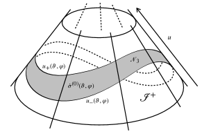
Impulsive data at future null infinity. In the shaded region $\mathcal{N}_{3}$, the time derivative of the asymptotic shear ${\sigma}^{(0)}(u,\vartheta,\varphi)$ is constant in $u$, everywhere else $\dot{\sigma}^{(0)}=0$.

If we consider such boundary data at future null infinity $\mathcal{I}^{+}$, we can embed them into Bondi coordinates $(u,r,\vartheta,\phi)$. The pulse starts at an asymptotic Bondi time $u_{-}(\vartheta,\varphi)$ and terminates at $u_{+}(\vartheta,\varphi)$ with total duration $(\Delta u)(\vartheta,\varphi)=u_{+}(\vartheta,\varphi)-u_{-}(\vartheta,\varphi)$. To leading order in the $1/r$-expansion, the map between the boundary intrinsic time coordinate $\mathcal{U}:\mathcal{N}_{3}\rightarrow[-1,1]$ and the asymptotic Bondi time $u$ is a mere angle-dependent dilation,

$$\partial^{a}_{\mathcal{U}}=\frac{(\Delta u)(\vartheta,\varphi)}{2}\partial^{a}_{u}+\mathcal{O}(r^{-1}).$$ (23)

Upon introducing an adapted Newman–Penrose tetrad $(k^{a},\ell^{a},m^{a},\bar{m}^{a})$, see [34], where $k^{a}=\partial^{a}_{r}$ and $\ell^{a}=\partial^{a}_{u}+\mathcal{O}(r^{-1})$, and both $k_{a}=-\nabla_{a}u$ and $\ell_{a}$ are surface orthogonal, we obtain the asymptotic expansion

$$\sigma_{(\ell)} =m^{a}m^{b}\nabla_{a}\ell_{b}=-\frac{\dot{\sigma}^{(0)}(u,\vartheta,\varphi)}{r}+\mathcal{O}(r^{-2}),$$ (24)

$$\sigma_{(k)} ={m}^{a}{m}^{b}\nabla_{a}k_{b}=\frac{\sigma^{(0)}(u,\vartheta,\varphi)}{r^{2}}+\mathcal{O}(r^{-3}).$$ (25)

The map (23) between the two clock variables implies a relationship between the asymptotic Bondi shear $\sigma^{(0)}$ and a family of radiative data $\{\sigma_{r}\}$ at the abstract boundary $\mathcal{N}_{3}$,

$$\sigma_{r}(\vartheta,\varphi)=\frac{(\Delta u)(\vartheta,\varphi)}{2}\frac{\dot{\sigma}^{(0)}(\vartheta,\varphi)}{r}+\mathcal{O}(r^{-2}).$$ (26)

This equation allows us to relate the asymptotic Bondi shear to the critical shear (22), where the Casimir changes its sign. Using the standard round metric at future null infinity $\mathcal{I}^{+}$, we then also have

$$E_{+}(\vartheta,\varphi)=E_{-}(\vartheta,\varphi)+\mathcal{O}(r^{1})=r^{2}+\mathcal{O}(r^{1}),$$ (27)

$$E_{-}(\vartheta,\varphi)-E_{+}(\vartheta,\varphi)=-4r(\Delta u)(\vartheta,\varphi)+\mathcal{O}(r^{0}).$$ (28)

We insert the expansion back into (22) and obtain the critical shear of the null generators $\partial_{\mathcal{U}}^{a}$

$$|\sigma_{\text{\it crit.}}|^{2}=\frac{1}{4}\frac{(\Delta u)^{2}(\vartheta,\varphi)}{\gamma^{2}+1}\frac{1}{r^{2}}+\mathcal{O}(r^{-3}).$$ (29)

We translate this value back into the asymptotic Bondi frame. Equation (26) implies that $\sigma_{\text{\it crit.}}$ corresponds to a critical value for the asymptotic shear given by

$$|\dot{\sigma}^{(0)}_{\text{\it crit.}}|=\frac{1}{\sqrt{\gamma^{2}+1}}+\mathcal{O}(r^{-1}).$$ (30)

Using the Bondi mass loss formula, we infer a critical value for the luminosity of the gravitational wave pulse,

$$\mathcal{L}_{\text{\it crit.}}=\frac{c^{5}}{4\pi G}\oint_{S_{2}}d^{2}\Omega\,|\dot{\sigma}^{(0)}_{\text{\it crit.}}|^{2}=\frac{\mathcal{L}_{\mathrm{P}}}{\gamma^{2}+1}.$$ (31)

If $L^{2}-c\bar{c}>0$, the impulsive wave will have a luminosity smaller than $\mathcal{L}_{\text{\it crit.}}$ In this regime, each light ray carries a discrete unitary representation of $SL(2,\mathbb{R})$. The fundamental operators are

$$c^{\dagger}|N,n_{a},n_{b},n_{c}\rangle=\mathrm{i}\sqrt{(N+n_{c})(n_{c}-N+1)}|N,n_{a},n_{b},n_{c}+1\rangle,$$ (32)

$$\mathopen{}\mathclose{{}\left(L^{2}-\tfrac{1}{2}(cc^{\dagger}+c^{\dagger}c)}\right)|N,n_{a},n_{b},n_{c}\rangle=N(N-1)|N,n_{a},n_{b},n_{c}\rangle,$$ (33)

$$a^{\dagger}|N,n_{a},n_{b},n_{c}\rangle=\sqrt{n_{a}+1}|N,n_{a}+1,n_{b},n_{c}\rangle,$$ (34)

$$b^{\dagger}|N,n_{a},n_{b},n_{c}\rangle=\sqrt{n_{b}+1}|N,n_{a},n_{b}+1,n_{c}\rangle,$$ (35)

where $n_{a}$ and $n_{b}$ are integers, $n_{c}=N,N+1,\dots$ is integer or half-integer and $N=1,\tfrac{3}{2},\dots$. Physical states are annihilated by the constraint (19). For the discrete series representations of $SL(2,\mathbb{R})$, a unique solution can be found by a linear combination of states

$$\bigl{\{}|N,n+r,r,N+m-r\rangle:r=0,\dots,m\bigr{\}}.$$ (36)

For the continuous series representations of $SL(2,\mathbb{R})$, $L^{2}-c\bar{c}<0$. The spectrum of the Casimir is continuous, for any $s\in\mathbb{R}$, we have

$$c^{\dagger}|s,n_{a},n_{b},n_{c}\rangle=\frac{1}{2\mathrm{i}}(\mathrm{i}s-2n_{c}-1)|s,n_{a},n_{b},n_{c}+1\rangle,$$

$$\mathopen{}\mathclose{{}\left(L^{2}-\tfrac{1}{2}(cc^{\dagger}+c^{\dagger}c)}\right)|s,n_{a},n_{b},n_{c}\rangle=-\frac{1}{4}(s^{2}+1)|s,n_{a},n_{b},n_{c}\rangle.$$ (37)

In this regime, the impulsive wave will have a luminosity bigger than $\mathcal{L}_{\text{\it crit.}}$ The spectrum of the Casimir is continuous, and the operator $L$ is no longer bounded from below. This has important consequences. The recurrence relations (19) will not terminate, physical states will be superpositions of kinematical states, where the quantum numbers $n_{a}$ and $n_{b}$ will become arbitrarily large. Therefore, the shear $\sigma\bar{\sigma}$ will be unbounded from above, see (18). If we take the Born rule and compute the probabilities for $\sigma\bar{\sigma}$ to take a certain value, there will always be a chance that an observer obtains $\sqrt{2\sigma\bar{\sigma}}>\pi/2$. In this case, the profile of the area density (10) will pass through a caustic, where $\Omega^{2}=0$. When there is a caustic, we violate the implicit assumption that we are in a smooth asymptotic region, in which $\Omega^{2}=r^{2}+\mathcal{O}(r)$, as $r\rightarrow\infty$. This can be avoided only when $L^{2}>c\bar{c}$, i.e. when the luminosity of the gravitational wave pulse is below $\mathcal{L}_{\text{\it crit.}}$. Then, the physical states are built from superpositions of the discrete series unitary representations of $SL(2,\mathbb{R})$ and for any physical state the quantum numbers $n_{a}$ and $n_{b}$ will be bounded from above.

4 Outlook and Conclusion

The critical luminosity (31) separates the continuous spectrum from the discrete eigenvalues of the $SL(2,\mathbb{R})$ Casimir. The bound depends on the Barbero–Immirzi parameter $\gamma$. This is a common feature in $D=4$. When $\gamma\neq 0$, the boundary charges are a mixture of electric and magnetic contributions that otherwise vanish in the $\gamma\rightarrow\infty$ limit [35, 11, 7]. The spectrum of the charges is determined by their algebraic properties alone, but the map between the charges and the physical observables depends on $\gamma$. In this way, the spectrum of physical observables can depend on $\gamma$. This is analogous to how the $\theta$-angle in quantum electrodynamics enters the Dirac quantization condition between magnetic and electric charges [36]. In loop quantum gravity, this effect is responsible for the quantization of geometric observables, such as area, angles, volumes and length [37, 38, 39, 40, 41]. Such a fundamental quantum discreteness of geometry affects other physical observables. It creates a fundamental bound on the energy density of matter [42, 43] and perhaps also acceleration [44]. Here, we found a similar bound on the gravitational wave luminosity (31). The analysis is based on a non-perturbative quantization of radiative data at finite distance. The result is only partial, because there is an implicit assumption: the validity of the classical asymptotic $1/r$-expansion when applied to the spectrum of gravitational observables at finite null boundaries. If the luminosity exceeds the critical luminosity (31), this assumption may no longer be valid due to the possible creation of caustics. What we have shown so far is only a first step. A more refined investigation will follow to understand the significance of the Planck power for the spectrum of the gravitational wave luminosity in non-perturbative quantum gravity.

References

- [1] C. W. Misner, K. S. Thorne, and J. A. Wheeler, Gravitation. W. H. Freeman, San Francisco, 1973.
- [2] V. Cardoso, T. Ikeda, C. J. Moore, and C.-M. Yoo, “Remarks on the maximum luminosity,” Phys. Rev. D 97 (2018), no. 8, 084013, arXiv:1803.03271.
- [3] A. Jowsey and M. Visser, “Reconsidering maximum luminosity,” Int. J. Mod. Phys. D 30 (2021), no. 14, 2142026, arXiv:2105.06650.
- [4] D. Keitel et al., “The most powerful astrophysical events: Gravitational-wave peak luminosity of binary black holes as predicted by numerical relativity,” Phys. Rev. D 96 (2017), no. 2, 024006, arXiv:1612.09566.
- [5] F. Zappa, S. Bernuzzi, D. Radice, A. Perego, and T. Dietrich, “Gravitational-Wave Luminosity of Binary Neutron Stars Mergers,” Phys. Rev. Lett. 120 (Mar, 2018) 111101, arXiv:1712.04267.
- [6] V. Cardoso, O. J. C. Dias, and J. P. S. Lemos, “Gravitational radiation in D-dimensional space-times,” Phys. Rev. D 67 (2003) 064026, arXiv:hep-th/0212168.
- [7] W. Wieland, “Quantum geometry of the null cone,” arXiv:2401.17491.
- [8] M. P. Reisenberger, “The symplectic 2-form for gravity in terms of free null initial data,” Class. Quant. Grav. 30 (2013) 155022, arXiv:1211.3880.
- [9] M. P. Reisenberger, “The Poisson brackets of free null initial data for vacuum general relativity,” Class. Quant. Grav. 35 (2018), no. 18, 185012, arXiv:1804.10284.
- [10] L. Ciambelli, L. Freidel, and R. G. Leigh, “Null Raychaudhuri: Canonical Structure and the Dressing Time,” arXiv:2309.03932.
- [11] W. Wieland, “Gravitational SL(2, ) algebra on the light cone,” JHEP 07 (2021) 057, arXiv:2104.05803.
- [12] J. Samuel, “A Lagrangian basis for Ashtekar’s formulation of canonical gravity,” Pramana 28 (1987) L429–L432, doi:10.1007/BF02847105.
- [13] T. Jacobson and L. Smolin, “The Left-Handed Spin Connection as a Variable for Canonical Gravity,” Phys. Lett. B 196 (1987) 39–42, doi:10.1016/0370-2693(87)91672-8.
- [14] S. Holst, “Barbero’s Hamiltonian derived from a generalized Hilbert-Palatini action,” Phys. Rev. D 53 (November, 1996) 5966–5969, arXiv:gr-qc/9511026.
- [15] J. F. Barbero G., “Real Ashtekar variables for Lorentzian signature space times,” Phys. Rev. D 51 (1995) 5507–5510, arXiv:gr-qc/9410014.
- [16] G. Immirzi, “Real and complex connections for canonical gravity,” Class. Quant. Grav. 14 (1997) L177–L181, arXiv:gr-qc/9612030.
- [17] A. Ashtekar and S. Speziale, “Horizons and Null Infinity: A Fugue in 4 voices,” arXiv:2401.15618.
- [18] A. Ashtekar, “New Variables for Classical and Quantum Gravity,” Phys. Rev. Lett. 57 (1986) 2244–2247, doi:10.1103/PhysRevLett.57.2244.
- [19] A. Raychaudhuri, “Relativistic Cosmology. I,” Phys. Rev. 98 (1955) 1123–1126, doi:10.1103/PhysRev.98.1123.
- [20] A. P. Balachandran, L. Chandar, and A. Momen, “Edge states in gravity and black hole physics,” Nucl. Phys. B 461 (1996) 581–596, arXiv:gr-qc/9412019.
- [21] S. Carlip, “Statistical mechanics of the (2+1)-dimensional black hole,” Phys. Rev. D 51 (1995) 632–637, arXiv:gr-qc/9409052.
- [22] G. Barnich and C. Troessaert, “BMS charge algebra,” JHEP 12 (2011) 105, arXiv:1106.0213.
- [23] W. Donnelly and L. Freidel, “Local subsystems in gauge theory and gravity,” JHEP 09 (2016) 102, arXiv:1601.04744.
- [24] S. Carrozza and P. A. Hoehn, “Edge modes as reference frames and boundary actions from post-selection,” JHEP 02 (2022) 172, arXiv:2109.06184.
- [25] L. Freidel, R. Oliveri, D. Pranzetti, and S. Speziale, “Extended corner symmetry, charge bracket and Einstein’s equations,” JHEP 09 (2021) 083, arXiv:2104.12881.
- [26] L. Freidel, M. Geiller, and D. Pranzetti, “Edge modes of gravity. Part I. Corner potentials and charges,” JHEP 11 (2020) 026, arXiv:2006.12527.
- [27] L. Freidel, M. Geiller, and D. Pranzetti, “Edge modes of gravity. Part II. Corner metric and Lorentz charges,” JHEP 11 (2020) 027, arXiv:2007.03563.
- [28] L. Freidel, M. Geiller, and W. Wieland, “Corner symmetry and quantum geometry,” in Handbook of Quantum Gravity, L. M. Cosimo Bambi and I. Shapiro, eds. Springer, 2023. arXiv:2302.12799.
- [29] W. Wieland, “Null infinity as an open Hamiltonian system,” JHEP 04 (2021) 095, arXiv:2012.01889.
- [30] W. Wieland, “Discrete gravity as a topological field theory with light-like curvature defects,” JHEP 05 (2017) 142, arXiv:1611.02784.
- [31] H. Bondi, M. G. J. van der Burg, and A. W. K. Metzner, “Gravitational waves in general relativity, VII. Waves from axi-symmetric isolated system,” Proc. of the Royal Soc. Lond. A: Mathematical, Physical and Engineering Sciences 269 (1962), no. 1336, 21–52, doi:10.1098/rspa.1962.0161.
- [32] R. Sachs, “Gravitational waves in general relativity VIII. Waves in asymptotically flat space-time,” Proceedings of the Royal Society London A 270 (1962), no. 1340, 103–126, doi:10.1098/rspa.1962.0206.
- [33] H. Bondi, “Gravitational Waves in General Relativity,” Nature 186 (1960), no. 4724, 535–535, doi:10.1038/186535a0.
- [34] E. Newman and R. Penrose, “An Approach to Gravitational Radiation by a Method of Spin Coefficients,” Journal of Mathematical Physics 3 (1962), no. 3, 566–578, doi:10.1063/1.1724257.
- [35] W. Wieland, “Fock representation of gravitational boundary modes and the discreteness of the area spectrum,” Ann. Henri Poincaré 18 (2017) 3695–3717, arXiv:1706.00479.
- [36] E. Witten, “Dyons of Charge ,” Phys. Lett. B 86 (1979) 283–287, doi:10.1016/0370-2693(79)90838-4.
- [37] C. Rovelli and L. Smolin, “Discreteness of area and volume in quantum gravity,” Nuclear Physics B 442 (1995), no. 3, 593–619, arXiv:gr-qc/9411005.
- [38] A. Ashtekar and J. Lewandowski, “Quantum theory of geometry I.: Area operators,” Class. Quant. Grav. 14 (1997) A55–A82, arXiv:gr-qc/9602046.
- [39] A. Ashtekar and J. Lewandowski, “Quantum Theory of Geometry II: Volume operators,” Advances in Mathematical and Theoretical Physics 1 (1997) 388–429, arXiv:gr-qc/9711031.
- [40] E. Bianchi, “The Length operator in Loop Quantum Gravity,” Nucl. Phys. B 807 (2009) 591–624, arXiv:0806.4710.
- [41] E. Bianchi and H. M. Haggard, “Discreteness of the volume of space from Bohr-Sommerfeld quantization,” Phys. Rev. Lett. 107 (2011) 011301, arXiv:1102.5439.
- [42] A. Ashtekar, T. Pawlowski, and P. Singh, “Quantum nature of the big bang,” Phys. Rev. Lett. 96 (2006) 141301, arXiv:gr-qc/0602086.
- [43] A. Ashtekar, T. Pawlowski, and P. Singh, “Quantum Nature of the Big Bang: Improved dynamics,” Phys. Rev. D 74 (2006) 084003, arXiv:gr-qc/0607039.
- [44] C. Rovelli and F. Vidotto, “Evidence for Maximal Acceleration and Singularity Resolution in Covariant Loop Quantum Gravity,” Phys. Rev. Lett. 111 (2013) 091303, arXiv:1307.3228.