Cross-Market Mergers with Common Customers:
When (and Why) Do They Increase Negotiated Prices?

Abstract

I examine the implications of cross-market mergers of suppliers to intermediaries that bundle products for consumers. These mergers are controversial. Some argue that suppliers’ products will be substitutes for intermediaries, despite not being substitutes for consumers. Others contend that because bundling makes products complements for consumers, products must be complements for intermediaries. I contribute to this debate by showing that two products can be complements for consumers but substitutes for intermediaries when the products serve a similar role in attracting consumers to purchase the bundle. This result leads to new recommendations and helps explain why cross-market hospital mergers raise prices.

Keywords: Cross-Market Mergers, Conglomerate Mergers, Bargaining, Hospital Mergers.

JEL classifications: D43, L13, L40.

1 Introduction

One of the most controversial current topics in merger enforcement is the competitive implications of cross-market hospital mergers in the United States. These mergers involve hospitals in distinct geographical areas or different diagnostic markets. The controversy stems from the fact that such transactions have been subject to little antitrust enforcement despite their prevalence and the existence of credible empirical evidence suggesting that they have led to increases in the reimbursement rates paid by insurers without corresponding increases in quality (Lewis and Pflum, 2015; Dafny, Ho and Lee, 2019; Brand and Rosenbaum, 2019).

This lack of enforcement, however, has not been due to a lack of scrutiny or regulatory neglect. Instead, authorities have concluded that such transactions do not raise antitrust concerns since hospitals operating in different markets are not substitutes for patients. The apparent contradiction between the empirical findings and antitrust practice has sparked interest among economists and practitioners alike, who, in recent years, have proposed alternative mechanisms to explain these increases in negotiated prices.

One theory that has gained increasing attention recently posits that hospitals can be substitutes for insurers—even if they are not substitutes for patients—in the presence of “common customers” (Vistnes and Sarafidis, 2013; Dafny, Ho and Lee, 2019). Common customers are purchasing entities—such as employers and households—that value the inclusion of multiple hospitals in the insurers’ network.

Nonetheless, this theory faces the challenge that the presence of common customers is equally consistent with hospitals being complements for the insurer, in which case the merger will lead to a reduction in negotiated prices (Brand and Rosenbaum, 2019). This is because hospitals in an insurer’s network offering non-overlapping services are likely complements for employers and households, making them complements for insurers as well. The previous argument is epitomized by Easterbrook et al. (2018, pp. 507-508) in the following example:

[Suppose there are] only two hospitals in an area—C and D… These two hospitals have no overlap in services… [However,] Because employers are likely to purchase health plans to meet the heterogeneous health needs of all of their employees… a plan with only hospital C or D may offer very limited value compared to a plan with both hospitals…

This would then generate complementarities across the hospitals to employers selecting an insurance plan to offer their employees… Complementarity between hospitals at the second stage of competition [i.e., when employers and insurers meet] in turn drives complementarity at the first stage [i.e., when insurers negotiate with hospitals].

The lack of a unified theory explaining these two different—and contradictory—results has increased calls for more research on the topic. For instance, Brand and Rosenbaum (2019) state that “a critical area for future research is to go beyond possibility results and recover how insurer profits change with network composition… determining how insurer profits shift with the inclusion and exclusion of different types of hospitals should be a priority.” My aim with this paper is to begin answering these calls.

More precisely, I analyze the effects of a merger of suppliers (e.g., two hospitals) that bargain with a single intermediary (e.g., an insurance company) over the carriage terms of products that are neither direct substitutes nor technological complements (e.g., because the hospitals operate in different markets). The intermediary bundles the products for sale to consumers interested in multiple products, making consumers “common customers” (e.g., they are employers looking for comprehensive health insurance plans for their employees). A consumer then purchases the bundle whenever the bundle’s expected net value exceeds the consumer’s private outside option.

Although the model is inspired by the debate on cross-market hospital mergers described above, it is general enough to encompass other relevant markets in which similar transactions have arisen. For instance, the model accommodates the retail industry equally well. In this market, consumer goods manufacturers, which sell their products through large retail chains offering one-stop shopping to consumers, have been consolidating during the last 20 years.

My main results are as follows. Consistent with the example in Easterbrook et al. (2018), the fact that consumers are common customers makes products in the bundle complementary to consumers even though these products are not direct complements or substitutes. However, I also show that Easterbrook et al.’s (2018) argument is incorrect in that these consumer-level complementarities do not always transfer upstream to the intermediary’s profit function. Thus, bundling can make two products complements for consumers—the common customers—but the products can still be substitutes for the intermediary. In this case, the merger of suppliers leads to higher negotiated prices.

The underlying reason behind this result is subtle yet intuitive. The starting point is realizing the dual role that products play in the intermediary’s bundle/lineup: products directly contribute with revenue/profits and indirectly contribute by attracting consumers to purchase the bundle (i.e., creating “consumer traffic”).

The widespread belief that consumer-level complementarities must drive complementarities upstream can be explained by the direct profit complementarities arising between two products in the intermediary’s bundle: Because products are complements for consumers, the inclusion of, for example, product C makes it more likely that the consumer purchases the bundle. This then increases the demand for, for example, product D, increasing the intermediary’s direct profits stemming from this last product.

The issue, however, is that the story does not end there. This is due to the fact that, since each product can help enhance consumers’ participation, both C and D can be used to increase the demand for other products in the intermediary’s lineup. Thus, C and D can potentially be substitutes in generating traffic for these additional products. If that is the case, and this substitutability in traffic dominates the direct profit complementarities described above, C and D will be substitutes for the intermediary in overall profits despite the two products being complements for the common customers.

I then focus on the antitrust implications of these results. First, I show that the theory provides a preliminary screening test that can immediately assess whether two products will be complements for the intermediary in overall profits.

In particular, if the intermediary’s bundle solely comprises the merging suppliers’ products or the merging products are weak complements in generating consumer traffic—in the sense that the sum of the reductions in the bundle’s sale from losing each product individually weakly exceeds the reduction in sales from losing them both jointly—then the products will necessarily be complements for the intermediary in overall profits. The beauty of this test is that the first condition can be observed directly from the intermediary’s portfolio, while the second condition can be readily assessed by empirically estimating the consumer loss ratios of the merging products.

Then, I show that even if two products fail this preliminary test so that the products can potentially, but not always, be substitutes for the intermediary, authorities can determine their complementarity/substitutability by assessing the role played by the products in the intermediary’s lineup. For instance, when two products mainly contribute to the intermediary by generating traffic, the products are likely to be substitutes in overall profits if they are substitutes in consumer traffic. In contrast, a product used to generate traffic and one used to extract profits will likely be complements in overall profits, even if they are substitutes in traffic.

Finally, I use my results to propose a new divestiture framework for these types of transactions. Indeed, suppose the merging suppliers offer portfolios of products instead of single products. Assume, furthermore, that these portfolios are known to be substitutes in overall profits, so the original transaction leads to an increase in negotiated prices. In that case, to offset the negative effects of a merger, authorities should force the merging parties to divest those products that contribute toward intermediaries’ overall profits mainly via consumer traffic.

This new divestiture approach, however, also comes with a note of caution: the divestiture of assets can backfire if authorities select the wrong products, i.e., those contributing to the intermediary via direct profits. This is because the divestiture then decreases the direct profit complementarities between the merging portfolios, making it more likely that the postdivestiture portfolios will be substitutable in traffic and, therefore, in overall profits.

1.1 Related Literature

This paper makes two important contributions to the literature on cross-market mergers of upstream suppliers. First, it shows that in the presence of common customers, two products can be substitutes for intermediaries despite being complements for customers. Second, my paper proposes new antitrust tools to deal with these types of transactions. I discuss the literature related to these contributions here.

My paper is connected to the work of Vistnes and Sarafidis (2013) and Dafny, Ho and Lee (2019), who propose the “holes in the network” theory of harm in the context of the healthcare industry to explain why cross-market hospital mergers can increase negotiated prices in the absence of foreclosure. The development of such a theory is important because in most cross-market hospital mergers in the United States, as well as in other conglomerate mergers, authorities have concluded that monopolization concerns were minimal.

Briefly, the “holes in the network theory” states that in the presence of common customers, two hospitals without overlapping services—for example, hospitals C and D—will be substitutes for an insurer in overall profits if customers continue to buy the plan without either hospital C or D but not without both (i.e., customers tolerate one but not two “holes” in the insurance plan).

As I formally show in Section 2.2, this theory is an extreme version of my argument. In particular, the theory describes a situation where C and D are “perfect substitutes” in creating traffic for the remaining items in the bundle. This explains why the insurer views C and D as substitutes in overall profits in this case.

Besides generalizing their results, my paper contributes to Vistnes and Sarafidis’s (2013) and Dafny, Ho and Lee’s (2019) theory in three important ways. First, neither paper addresses the apparent contradiction—raised by Easterbrook et al. (2018) and Brand and Rosenbaum (2019)—of products being complements for customers but substitutes for intermediaries. By providing a unifying framework, my paper shows that there is, in fact, no contradiction and clarifies under what conditions complementarities at the customer level transfer to the intermediary level.

Second, neither Vistnes and Sarafidis (2013) nor Dafny, Ho and Lee (2019) make the connection between the complementarity/substitutability of products at the intermediary level and the role those products play in the intermediary’s lineup. This is the key insight behind the new divestiture approach I develop here. Third and finally, my general framework leads to new antitrust tools to deal with these transactions: a preliminary test to screen whether two products are complements for intermediaries and the aforementioned divestiture framework.

My paper is also related to the work by Peters (2014). He provides a different theoretical mechanism for explaining how cross-market mergers of upstream suppliers can increase negotiated prices in the presence of common customers. Unlike my theory, Peters’s (2014) theory posits that mergers can raise prices even when products are not substitutes for intermediaries. Specifically, he argues that cross-market mergers can increase suppliers’ reservation payoffs in negotiations with intermediaries when intermediaries compete.

Concerning this alternative theory, in the online Appendix, I provide an extension that combines this mechanism and mine. There, I show that the two effects operate under different circumstances and provide a preliminary screening test—similar to the one I propose to screen for complementarities at the intermediary level—that can be used to assess whether this additional effect is present in a given merger.

2 A Simple Model

In this section, I present my main results in a simplified model. In this model, I work with reduced-form payoffs (instead of dealing with retail and wholesale prices and marginal costs) and assume that the intermediary and the suppliers bargain over lump-sum fees. The latter implies that upstream mergers will only affect firms’ profits, not consumer surplus.

In Section 3, I fully microfound this simplified setting and consider negotiations over linear contracts (as in, e.g., Crawford and Yurukoglu, 2012; Ho and Lee, 2017; Crawford et al., 2018; Luco and Marshall, 2020). There I show that the simple model’s lessons remain unchanged with the exception that consumer welfare is impacted.

2.1 The Setting

Setup.— Suppose the intermediary is a large monopoly retail chain offering one-stop shopping to a unit mass of infinitesimal consumers (below, I show that this model can be directly reinterpreted as one depicting the healthcare market). This intermediary can potentially carry three products, $i\in\{0,1,2\}$, that are neither direct substitutes nor technological complements (i.e., they are “unrelated” in consumption). Each product, moreover, is solely produced by a single supplier (hence, I can refer to products or suppliers indistinguishably).

Suppliers can only reach final consumers indirectly via the intermediary. Consumers have a unit demand for each product. I assume—in a reduced-form fashion—that purchasing a unit of product $i$ gives the consumer a surplus of $v_{i}\geq 0$, while it generates profits of $\pi_{i}\geq 0$ and $\varphi_{i}\geq 0$ to the intermediary and supplier $i$, respectively. Because products are unrelated, when the consumer buys multiple products, her surplus—and the firms’ profits—are additive over these products.

When visiting the intermediary, consumers also incur a shopping cost $\xi\geq 0$. The latter is heterogeneous among the population of consumers and is characterized by the cumulative distribution function $G(\xi)$. I assume that consumers observe the intermediary’s portfolio of products before deciding whether to incur $\xi$. This shopping cost could be interpreted literally as the opportunity cost of time spent in traffic and parking, selecting products, and so forth, or—taking a partial equilibrium view—as the value for the consumer of visiting its best alternative among the intermediary’s competitors.

Finally, I assume that the intermediary and the suppliers bargain over the term of carriage. More precisely, each supplier engages in a bilateral Nash bargain with the intermediary over a lump-sum fee, anticipating that the other suppliers will also reach an agreement with the intermediary.

Payoffs.— Let $\mathcal{N}\equiv\{0,1,2\}$ be the set of all products/suppliers. The indirect utility function of a consumer with a shopping cost of $\xi$ if the intermediary’s portfolio is $\mathcal{G}\in 2^{\mathcal{N}}$ is given by $U(\mathcal{G};\xi)=\max\{\sum_{i\in\mathcal{G}}v_{i}-\xi,0\}$. The overall demand for product $i$, in turn, is equal to the fraction of consumers visiting the intermediary:

$$D_{i}(\mathcal{G})=\mathbbm{1}_{i\in\mathcal{G}}\mathbb{P}\big{(}\textstyle\sum_{j\in\mathcal{G}}v_{j}\geq\xi\big{)}=\mathbbm{1}_{i\in\mathcal{G}}\tilde{G}(\mathcal{G})$$ (1)

where for future reference, $\tilde{G}:2^{\{\emptyset,0,1,2\}}\to[0,1]$ defined as $\tilde{G}(\mathcal{G})\equiv G(\textstyle\sum_{i\in\mathcal{G}}v_{i})$ is the consumer traffic function and $\mathbbm{1}_{X}$ denotes the indicator function of the event $X$. Thus, the profits before negotiated fees made by the supplier of product $i$ are equal to $\Phi_{i}(\mathcal{G})=\varphi_{i}D_{i}(\mathcal{G})=\varphi_{i}\mathbbm{1}_{i\in\mathcal{G}}\tilde{G}(\mathcal{G})$. On the other hand, since the intermediary makes a per-consumer profit of $\mathbbm{1}_{i\in\mathcal{G}}\pi_{i}$ on product $i$, its overall profits before fees are equal to:

$$\Psi(\mathcal{G})=\big{(}\textstyle\sum_{i\in\mathcal{G}}\pi_{i}\big{)}\tilde{G}(\mathcal{G})$$ (2)

Remark 1: Consumer Level Complementarities. The setting described exhibits complementarities at the consumer level. More precisely, the indirect utility of a consumer with shopping cost $\xi$, $U(\mathcal{G};\xi)$, is supermodular in the inclusion of products in the bundle (see Appendix A for the formal proof of this result). This, in turn, makes products gross complements when considering the intermediary’s demand, in the sense that $i$’s demand, $D_{i}(\mathcal{G})$, is increasing in the cardinality of the intermediary’s product portfolio $\mathcal{G}$. Intuitively, the complementarity between products at the consumer level arises due to one-stop shopping economies.

Remark 2: Healthcare Interpretation. The model presented above can be directly reinterpreted as one depicting the healthcare market. Under this interpretation, $v_{i}$ is the total surplus that all the employees of a given employer receive from having access to hospital $i$. An employer will then offer the intermediary’s insurance plan to their employees if the total surplus employees receive from having access to the plan, $\sum_{i\in\mathcal{G}}v_{i}$, exceeds the administrative cost or outside option $\xi\in\mathbb{R}_{+}$.

Note that under this interpretation, the “consumer” choosing whether to “visit the intermediary” is different from the one “consuming” the product. The former is the employer (the “common customer” in this setting), while the latter is the employer’s employees. Thus, under this interpretation, complementarities between hospitals arise at the employer level, not at the employee/patient level, and are explained by employers looking to “purchase health plans to meet the heterogeneous health needs of all of their employees” (as stated in the example by Easterbrook et al., 2018, quoted in the Introduction).

2.2 The Effects of an Upstream Merger

I now analyze how the merger of suppliers $1$ and $2$ affects the terms negotiated with the intermediary. Before the merger, the negotiated lump-sum fee paid by the intermediary to supplier $i$, denoted by $t_{i}^{\text{pre}}$, solves the following Nash bargaining problem:

$$t_{i}^{\text{pre}}=\operatorname*{arg\,max}_{t_{i}}\left[\Psi(\mathcal{N})-\Psi(\mathcal{N}\setminus\{i\})-t_{i}\right]\times\left[\Phi_{i}(\mathcal{N})+t_{i}\right]$$

where for simplicity, I have assumed that the intermediary and supplier $i$ both have bargaining weights equal to $1/2$ (as shown in Section 3, this assumption does not affect the results). Hence, the combined premerger payments that suppliers $1$ and $2$ can secure are equal to:

$$\textstyle T^{\text{pre}}=\sum_{i=1,2}t_{i}^{\text{pre}}=\sum_{i=1,2}\Big{(}\Psi(\mathcal{N})-\Psi(\mathcal{N}\setminus\{i\})-\Phi_{i}(\mathcal{N})\Big{)}\Big{/}2$$ (3)

Suppose now that suppliers $1$ and $2$ merge. To highlight my results most transparently, I assume that there are no cost efficiencies or synergies related to the merger. Consequently, the newly negotiated terms for each supplier within the conglomerate $\mathcal{U}=\{1,2\}$ (where $\mathcal{U}$ stands for “union” or “merger”) must solve the following reformulated Nash bargaining problem:

$$\textstyle\bm{t}^{\text{post}}=\operatorname*{arg\,max}_{(t_{1},t_{2})}\left[\Psi(\mathcal{N})-\Psi(\mathcal{N}\setminus\mathcal{U})-\sum_{i=1,2}t_{i}\right]\times\left[\sum_{i=1,2}\big{(}\Phi_{i}(\mathcal{N})+t_{i}\big{)}\right]$$

where I have assumed—as in Crawford and Yurukoglu (2012), Gowrisankaran, Nevo and Town (2015), Ho and Lee (2017), and Dafny, Ho and Lee (2019)—that upon disagreement with any given merging supplier, the intermediary loses the products of the entire conglomerate. The first-order condition of this problem yields:

$$\textstyle T^{\text{post}}=\sum_{i=1,2}t_{i}^{\text{post}}=\bigg{(}\Psi(\mathcal{N})-\Psi(\mathcal{N}\setminus\mathcal{U})-\sum_{i=1,2}\Phi_{i}(\mathcal{N})\bigg{)}\bigg{/}2$$ (4)

Comparing (3) and (4), the total payment to the conglomerate will be greater than the sum of premerger payments (i.e., $T^{\text{post}}>T^{\text{pre}}$) if the merging products are substitutes for the intermediary in terms of overall profits:

$$\textstyle\Psi(\mathcal{N})-\Psi(\mathcal{N}\setminus\mathcal{U})>\sum_{i=1,2}\Big{(}\Psi(\mathcal{N})-\Psi(\mathcal{N}\setminus\{i\})\Big{)}$$ (5)

That is, if the loss in profits for the intermediary when simultaneously losing both products exceeds the sum of the loss from losing each product separately.

As noted by Dafny, Ho and Lee (2019), this condition will typically be satisfied if products are direct substitutes for consumers. In the current setting, however, this is not the case. Nevertheless, the “holes in the network” theory for harm argues that products can still be substitutes for the intermediary, given that consumers are interested in multiple products (i.e., they are “common customers”). If true, a merger of suppliers $1$ and $2$ should lead to higher negotiated prices.

The problem with this theory—as pointed out by Brand and Rosenbaum (2019)—is that products are, in fact, complements for consumers (see Remark 1). Because these consumer-level complementarities must transfer upstream (Easterbrook et al., 2018), the latter implies that products must be complements—not substitutes—for the intermediary in terms of profits (i.e., the inequality (5) is reversed). Thus, the merger of suppliers $1$ and $2$ should lead to lower—not higher—negotiated prices.

Which is it, then? Are products complements or substitutes for the intermediary? And how can we square the existence of consumer-level complementarities with the “holes in the network” theory of harm that argues that two products can sometimes be substitutable for the intermediary in this context?

To try settling this debate, evaluate (2) on (5). Rearranging terms, one obtains that products $1$ and $2$ will be substitutes for the intermediary in overall profits (i.e., (5) holds) if and only if:

$$\pi_{0}\big{[}\tilde{G}(\mathcal{N})-\tilde{G}(\mathcal{N}\setminus\mathcal{U})-\textstyle\sum_{i=1,2}\big{(}\tilde{G}(\mathcal{N})-\tilde{G}(\mathcal{N}\setminus\{i\})\big{)}\big{]}\\ >\pi_{1}\big{[}\tilde{G}(\mathcal{N})-\tilde{G}(\mathcal{N}\setminus\{2\})\big{]}+\pi_{2}\big{[}\tilde{G}(\mathcal{N})-\tilde{G}(\mathcal{N}\setminus\{1\})\big{]}$$ (6)

This is the key equation of this paper; it summarizes the heart of my contribution.

The right-hand side of (6)—which is always positive—represents the direct profit complementarities that arise between products $1$ and $2$ in the intermediary’s profit function. This complementarity is explained because carrying product $1$ increases the number of consumers visiting the intermediary and, therefore, increases the intermediary’s direct profits stemming from product $2$ (and vice versa). The stronger this complementarity of direct profits is, the less likely it will be that (6) holds. This side of equation (6) is the source of the widespread belief that consumer-level complementarities must also drive complementarities upstream.

The left-hand side of (6), in turn, represents the complementarity or substitutability between the merging products in generating traffic for product $0$, the product that is not involved in the transaction. In particular, products $1$ and $2$ will be substitutes in generating traffic for product $0$ if the intermediary’s loss in terms of consumer traffic from simultaneously losing both products exceeds the sum of the reductions from losing each product individually:

$$\tilde{G}(\mathcal{N})-\tilde{G}(\mathcal{N}\setminus\mathcal{U})>\textstyle\sum_{i=1,2}\big{(}\tilde{G}(\mathcal{N})-\tilde{G}(\mathcal{N}\setminus\{i\})\big{)}$$ (7)

When that is the case, the left-hand side of (6) will also be positive. Intuitively, products $1$ and $2$ can be substitutes in generating traffic for product $0$, because each product can individually be used to increase overall consumer traffic. The stronger this substitutability in traffic is, or the higher the direct profits stemming from product $0$ are, the more likely it will be that (6) holds.

Thus, if the merging products are substitutes in traffic and this substitutability is strong enough, the products can be complements for consumers but substitutes for the intermediary in overall profits. When this happens, the merger of suppliers $1$ and $2$ leads to higher negotiated prices, just as the “holes in the network” theory of harm predicts.

Proposition 1.

The merger of suppliers $1$ and $2$ can lead to higher negotiated prices despite complementarities at the consumer level. A necessary condition for this to occur is for the merging products to be substitutes in generating consumer traffic.

Proof.

Immediate from the discussion above. ∎

In fact, it is easy to see that the “holes in the network” theory is an extreme version of my argument. Indeed, recall that according to this theory, two products will be substitutes for the intermediary when all consumers are willing to purchase the bundle when one of the products is missing but not when both are. That is, if $\tilde{G}(\mathcal{N})=\tilde{G}(\mathcal{N}\setminus\{i\})=1$ for $i=1,2$ and $\tilde{G}(\mathcal{N}\setminus\mathcal{U})=0$, in which case (6) is always satisfied as it becomes:

$$\overbrace{\pi_{0}\big{[}\tilde{G}(\mathcal{N})-\tilde{G}(\mathcal{N}\setminus\mathcal{U})-\textstyle\sum_{i=1,2}\big{(}\tilde{G}(\mathcal{N})-\tilde{G}(\mathcal{N}\setminus\{i\})\big{)}\big{]}}^{=\pi_{0}}\\ >\underbrace{\pi_{1}\big{[}\tilde{G}(\mathcal{N})-\tilde{G}(\mathcal{N}\setminus\{2\})\big{]}+\pi_{2}\big{[}\tilde{G}(\mathcal{N})-\tilde{G}(\mathcal{N}\setminus\{1\})\big{]}}_{=0}$$

Intuitively, if none of the consumers stop purchasing the bundle when either C or D is missing, but all stop purchasing it when both C and D are missing, the two products are, in essence, “perfect substitutes” in creating traffic for the remaining items in the bundle. Moreover, because adding either product to the bundle does not affect the bundle’s sales when the other product is present, C and D create no direct profit complementarities to each other.

Thus, the situation described by this theory minimizes direct profit complementarities among merging products and maximizes their substitutability in creating traffic for other items in the intermediary’s lineup. This explains why the intermediary always sees the merging products as substitutes in terms of profits in this case. Equation (6) shows, however, that such an extreme situation is not necessary for the merger to increase negotiated prices; it is only sufficient. Much milder forms of substitutability in traffic can also lead to increases in negotiated prices.

2.3 Some Novel Antitrust Implications

I now turn my attention to the antitrust implications of these results. First, equation (6) immediately provides two different sufficient conditions that guarentee that a given merge will not increase negotiated prices.

Proposition 2.

If either:

• The intermediary’s bundle solely comprises the merging suppliers’ products, i.e., product $0$ does not exist.

• Or the merging products are weak complements in generating traffic, i.e.,

  $$\textstyle\sum_{i=1,2}\big{(}\tilde{G}(\mathcal{N})-\tilde{G}(\mathcal{N}\setminus\{i\})\big{)}\geq\tilde{G}(\mathcal{N})-\tilde{G}(\mathcal{N}\setminus\mathcal{U})$$ (8)

Then products $1$ and $2$ are necessarily weak complements for the intermediary in overall profits, and the proposed merger does not increase negotiated prices.

Proof.

For (i), note that if product $0$ does not exist, then (6) becomes:

$$0>\pi_{1}\big{[}\tilde{G}(\mathcal{N})-\tilde{G}(\mathcal{N}\setminus\{2\})\big{]}+\pi_{2}\big{[}\tilde{G}(\mathcal{N})-\tilde{G}(\mathcal{N}\setminus\{1\})\big{]}$$

which is never satisfied as the right-hand side is always weakly positive (note that the same occurs if $\pi_{0}=0$). For (ii), note that if (8) holds, then (6) is necessarily violated, as its left-hand side is weakly negative and the right-hand side is weakly positive. ∎

Intuitively, if the intermediary’s bundle solely comprises the merging parties’ products, whether the products are substitutes or complements in generating traffic for other products in the intermediary’s lineup is irrelevant; only the direct profits complementarities between the two merging products matter. On the other hand, if the merging products are weak complements in generating traffic, they are complements in the two dimensions that matter for the intermediary’s profit function: direct profits and traffic. Hence, the products must necessarily be complements for the intermediary regarding overall profits as well.

These two sufficient conditions can then be used as a first-pass test to immediately assess whether two products will be complements for the intermediary in terms of profits. The beauty of this test is that the first condition can be observed directly from the intermediary’s portfolio, while the second condition can be readily assessed by empirically estimating the consumer loss ratios of the merging products.

However, suppose two products in the intermediary’s lineup fail the test; thus, the products can potentially, but not necessarily, be substitutes for the intermediary in terms of profits. Is there another way for authorities to assess their complementarity or substitutability for the intermediary? The answer is positive. The key is to look at the products’ role in the intermediary’s lineup.

To do this, let me begin by providing two definitions: product $i$ is said to be a “pure” profit contributor if $v_{i}=0$ and $\pi_{i}>0$, while it is said to be a “pure” traffic generator if $\pi_{i}=0$ and $v_{i}>0$. Intuitively, pure profit contributors only contribute to the intermediary’s overall profits with direct profits, while pure traffic generators only contribute by creating consumer traffic. With these labels in mind, I can then state the following proposition:

Proposition 3.

Suppose that $\pi_{0}>0$ and that $\tilde{G}(\cdot)$ is submodular in the products carried by the intermediary (so two products are always substitutes in generating traffic for a third unrelated product).

• If product $1$ is a pure profit contributor and product $2$ a pure traffic generator (or vice versa), the products are complements for the intermediary in terms of overall profits.

• If products $1$ and $2$ are pure traffic generators, the products are substitutes for the intermediary in terms of overall profits.

Proof.

Consider a pure profit contributor with a pure traffic generator, i.e., $(\pi_{1}>0,v_{1}=0)$ and $(\pi_{2}=0,v_{2}>0)$. Then, $\tilde{G}(\mathcal{N})=\tilde{G}(\mathcal{N}\setminus\{1\})=G(v_{0}+v_{2})$ and $\tilde{G}(\mathcal{N}\setminus\{2\})=\tilde{G}(\mathcal{N}\setminus\mathcal{U})=G(v_{0})$. The left-hand side of (6) is then equal to zero, while its right-hand side is equal to $\pi_{1}[G(v_{0}+v_{2})-G(v_{0})]>0$. Thus, condition (6) is violated, so the products are complements for the intermediary in terms of profits.

Consider, in turn, two pure traffic generators, i.e., $(\pi_{1}=0,v_{1}>0)$ and $(\pi_{2}=0,v_{2}>0)$. Then, the right-hand side of (6) is zero, while the left-hand side of (6) is equal to:

$$\pi_{0}\left[\tilde{G}(\mathcal{N})-\tilde{G}(\mathcal{N}\setminus\mathcal{U})-\textstyle\sum_{i=1,2}\big{(}\tilde{G}(\mathcal{N})-\tilde{G}(\mathcal{N}\setminus\{i\})\big{)}\right]\\ =\pi_{0}\left[G(v_{0}+v_{1})+G(v_{0}+v_{2})-G(v_{0}+v_{1}+v_{2})-G(v_{0})\right]$$

This last term is positive if $\tilde{G}(\cdot)$ is submodular in the products included in the bundle. Thus, condition (6) is satisfied, and the products are substitutes for the intermediary in terms of profits.∎

Intuitively, two pure traffic generators do not generate direct profit complementarities to each other, as their direct profit contributions are nonexistent. Hence, only their substitutability in traffic matters when determining whether they are complements or substitutes for the intermediary. In contrast, a pure profit contributor does not “compete” in consumer traffic with a traffic generator, as the profit contributor does not generate traffic. Therefore, the two products are complements in overall profits to the intermediary, as only direct profit complementarities are present.

In reality, no product will ever be a pure profit contributor or a pure traffic generator; products typically contribute with direct profits and consumer traffic. However, simple continuity arguments imply that the results of Proposition 3 extend beyond the limit cases considered there.

For a concrete example, suppose that $(\pi_{i},v_{i})\in[0,\bar{\pi}]\times[0,\bar{v}]$ for $i=0,1,2$. Rhodes, Watanabe and Zhou (2021) show how a relatively general family of demand functions can generate this space (and below, I discuss what determines a product’s position in it). Building on the intuition of Proposition 3, Figure 2 depicts the mergers that would increase negotiated prices for a given set of parameters.

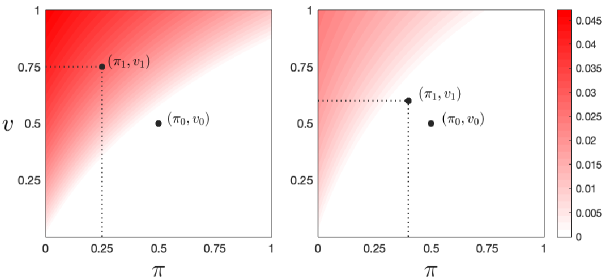
Figure 1: Mergers that Increase Prices According to the $(\pi,v)$ Space

Notes. In the figure, $\bar{\pi}=\bar{v}=1$. The first panel has $(\pi_{1},v_{1})=(\nicefrac{{1}}{{4}},\nicefrac{{3}}{{4}})$, while the second panel has $(\pi_{1},v_{1})=(\nicefrac{{1}}{{3}},\nicefrac{{2}}{{3}})$. Remaining Parameters: $(\pi_{0},v_{0})=(\nicefrac{{1}}{{2}},\nicefrac{{1}}{{2}})$, $G(\xi)=1-e^{-\lambda\xi}$ with $\lambda=\nicefrac{{3}}{{2}}$.

More precisely, keeping $(\pi_{0},v_{0})$ and $(\pi_{1},v_{1})$ fixed, and for $G(\xi)=1-e^{-\lambda\xi}$ (so that $\tilde{G}(\cdot)$ is submodular in the products carried by the intermediary), the colored regions in the panels represent all the combinations $(\pi_{2},v_{2})$ so that $T^{\text{post}}-T^{\text{pre}}>0$. Moreover, the darker the color, the more pronounced the price increase (i.e., the higher $T^{\text{post}}-T^{\text{pre}}$). As the figure shows, the more problematic mergers arise when both $(\pi_{1},v_{1})$ and $(\pi_{2},v_{2})$ are located towards the northwest corner of the unit square. These are mergers of products that contribute little to the intermediary’s overall profit via direct profits and significantly via consumer traffic.

The only remaining question—the elephant in the room—is what determines the role different products play in the intermediary’s lineup. As shown by Rhodes, Watanabe and Zhou (2021), and Ide and Montero (2023), products’ locations in the $(\pi,v)$ space are intimately connected to the shape of products’ demand. In particular, products with “more concave” and “rectangular-shaped” demands will have a higher $\pi_{i}/v_{i}$ ratio.

Intuitively, with more concave and rectangular-shaped demands, the intermediary can extract a larger share of consumer surplus without introducing significant monopoly distortions. As a result, the intermediary uses those products mainly as profit contributors, leading to a higher $\pi_{i}/v_{i}$ ratio. Conversely, the more convex a product’s demand is, the more expensive it is to extract consumer surplus in terms of monopoly distortions. Thus, the intermediary tends to use those products primarily as traffic generators. I will illustrate this intuition in more detail in Section 3, once I introduce the full-fledged model.

Based on this understanding, it can be conjectured that highly specialized hospitals primarily serve as traffic generators in an insurer’s network. This is due to the fact that, for such hospitals, the option value of having access to their services holds significant importance for patients, resulting in highly convex demands. In contrast, routine healthcare providers, which offer a wide range of routine procedures, are likely to be predominantly utilized by insurers to generate direct profits, as their demand curves are expected to be more concave and rectangular-shaped.

Consequently, my findings suggest that authorities should pay particular attention to transactions involving two or more specialized healthcare providers or cases where a large hospital system acquires a highly specialized provider.

2.4 A New Divestiture Framework

Proposition 3 and Figure 1 also have an additional implication. If we interpret suppliers’ offerings as portfolios of products instead of single products, they lead to a new divestiture framework for these transactions. In particular, they imply that to offset the negative effects of a merger, authorities should force the merging entities to divest those products located in the northwest corner of the $(\pi,v)$ space.

To see this point more formally, suppose that $\tilde{G}(\cdot)$ is submodular and that there is an additional product in the market, product $3$. The latter product is also manufactured by a single supplier, supplier $3$. Furthermore, assume that suppliers $1$ and $2$ have already merged to form conglomerate $\mathcal{U}=\{1,2\}$ and are now considering acquiring supplier $3$.

As before, denote by $\mathcal{N}\equiv\{0,1,2,3\}$ the set of all products in the market, and let $T^{\text{pre}}\equiv\sum_{i=1,2,3}t_{i}^{\text{pre}}$ and $T^{\text{post}}\equiv\sum_{i=1,2,3}t_{i}^{\text{post}}$ be the merging parties’ combined pre- and postmerger profits. Define also $\Delta T(\text{no divestiture})$, $\Delta T(\text{divest}\ 1)$, and $\Delta T(\text{divest}\ 2)$ as the change in the merging parties’ profits due to the merger, $\Delta T\equiv T^{\text{post}}-T^{\text{pre}}$, if:

• No divestiture remedy is imposed.

• $\mathcal{U}$ must divest product $1$ as a condition to acquire $3$.

• $\mathcal{U}$ must divest product $2$ as a condition to acquire $3$.

As I show in Appendix B, the relationship between $\Delta T(\text{no divestiture})$, $\Delta T(\text{divest}\ 1)$, and $\Delta T(\text{divest}\ 2)$ is:

$$\textstyle\Delta T(\text{divest}\ 1)=\Delta T(\text{no divestiture})$$

$$\qquad\ \ \ -\frac{1}{2}\underbrace{\left[\Psi(\mathcal{N})-\Psi(\mathcal{N}\setminus\{1,2,3\})-\big{(}\Psi(\mathcal{N})-\Psi(\mathcal{N}\setminus\{1\})\big{)}-\big{(}\Psi(\mathcal{N})-\Psi(\mathcal{N}\setminus\{2,3\})\big{)}\right]}_{\text{degree of substitutability in profits between product $1$ and portfolio $\{2,3\}$ }}$$

$$\textstyle\Delta T(\text{divest}\ 2)=\Delta T(\text{no divestiture})$$

$$\qquad\ \ \ -\frac{1}{2}\underbrace{\left[\Psi(\mathcal{N})-\Psi(\mathcal{N}\setminus\{1,2,3\})-\big{(}\Psi(\mathcal{N})-\Psi(\mathcal{N}\setminus\{2\})\big{)}-\big{(}\Psi(\mathcal{N})-\Psi(\mathcal{N}\setminus\{1,3\})\big{)}\right]}_{\text{degree of substitutability in profits between product $2$ and portfolio $\{1,3\}$ }}$$

These expressions have two important implications. First, forcing $\mathcal{U}$ to divest product $1$ is more effective than forcing it to divest product $2$—in the sense that it leads to a lower increase in negotiated payments—when the degree of substitutability in profits between product $1$ and portfolio $\{2,3\}$ is higher than the substitutability in profits of product $2$ and portfolio $\{1,3\}$. This will typically be the case when product $1$ is located closer to the northwest corner of the $(\pi,v)$ space than product $2$, as the following example illustrates:

Example 1. Suppose that products $1$ and $3$ are pure traffic generators, $(\pi_{1}=0,v_{1}>0)$ and $(\pi_{3}=0,v_{3}>0)$, while product $2$ is a pure profit contributor, $(\pi_{2}>0,v_{2}=0)$. The degree of substitutability in profits between product $1$ and portfolio $\{2,3\}$ is:

$$\pi_{0}\big{[}G(v_{0}+v_{1})+G(v_{0}+v_{3})-G(v_{0}+v_{1}+v_{3})-G(v_{0})\big{]}-\pi_{2}\big{[}G(v_{0}+v_{1}+v_{3})-G(v_{0}+v_{3})\big{]}$$

while the degree of substitutability in profits between product $2$ and portfolio $\{1,3\}$ is:

$$\pi_{2}[G(v_{0})-G(v_{0}+v_{1}+v_{3})]$$

Thus, product $1$ and portfolio $\{2,3\}$ have a higher degree of substitutability than product $2$ and portfolio $\{1,3\}$ given that:

$$G(v_{0}+v_{1})+G(v_{0}+v_{3})-G(v_{0}+v_{1}+v_{3})-G(v_{0})>0\quad\text{and}\quad G(v_{0}+v_{3})>G(v_{0})$$

Consequently, to offset the increases in negotiated payments arising due to $\mathcal{U}$’s acquisition of product $3$, an authority should aim its divestiture efforts toward product $1$—the traffic generator—rather than toward product $2$—the profit contributor.

The second important implication is that if authorities force the merging entities to divest the wrong products (i.e., those originally located at the southeast corner of the $(\pi,v)$ space), the policy can backfire. This is because the divestiture negatively impacts the direct profit complementarities between portfolios, making it more likely that the postdivestiture portfolios will be substitutable in traffic. The previous point can be seen in the above example, where products $1$ and $3$ are pure traffic generators and product $2$ is a pure profit contributor:

Example 1 (Continued). The degree of substitutability in profits between product $2$ and portfolio $\{1,3\}$ in this case is equal to $\pi_{2}[G(v_{0})-G(v_{0}+v_{1}+v_{3})]$. The latter is strictly negative—that is, portfolios $2$ and $\{1,3\}$ are complements in profits for the intermediary—implying that $\textstyle\Delta T(\text{divest}\ 2)>\Delta T(\text{no divestiture})$.

The divestiture approach outlined above is novel and differs significantly from the ones used in practice. For instance, in the 2005 cross-market/conglomerate merger involving Procter & Gamble and Gillette, the European Commission forced P&G to divest its battery toothbrush business “SpinBrush,” since there were significant horizontal overlaps at the consumer level between this brand and Gillette’s “OralB” brand.

In other words, the remedy focused on eliminating any horizontal overlaps as viewed from the perspective of final consumers: SpinBrush and OralB were direct “head-to-head” rivals at the point of sale. In contrast, the divestiture measures presented here aim to tackle the more subtle “horizontal overlap” arising at the intermediary’s level when two portfolios of products are “substitutes” in generating traffic for other items in the intermediary’s lineup, even though the products belonging to these portfolios are not direct rivals at the point of sale.

This finishes the presentation of the article’s main results. In the next section, I microfound the model presented above and show that the results remain unchanged.

3 Microfounding the Simple Model

I now microfound the result of the previous section by employing a model inspired by Ho and Lee (2017) and Ide and Montero (2023).

3.1 Setup

Products, Suppliers, and Technology.— There is a set $\mathcal{N}=\{1,...,n\}$ of products (where $n\geq 2$), each produced by a single supplier (thus I can continue referring to suppliers or products indistinguishably).

To manufacture product $i\in\mathcal{N}$, the corresponding supplier uses a constant-returns-to-scale technology. To avoid introducing merger synergies on the technological side, I assume that production technologies are separable across the different products. Thus, the marginal cost of producing $i\in\mathcal{N}$, denoted by $c_{i}\geq 0$, is independent of the ownership structure of the upstream market.

The Intermediary.— There is a single monopoly intermediary that buys products from suppliers and resells them to consumers. This intermediary sets retail prices for the products it carries. Moreover, it has no operating costs beyond purchasing the products from suppliers.

Conglomerates.— Each supplier originally belongs to one of $m$ conglomerates, where $2\leq m\leq n$. The set of all conglomerates is denoted by $\bm{\mathcal{C}}=\{\mathcal{C}_{1},...,\mathcal{C}_{m}\}$. Note that conglomerate $j$ can also represent a single supplier if $|\mathcal{C}_{j}|=1$.

The intermediary must carry all or none of the products of a given conglomerate, although it can negotiate different terms with each supplier within the conglomerate. I also assume that all the suppliers belonging to the same conglomerate perfectly internalize each other’s profits.

Final Consumers.— There is a unit mass of final consumers. They wish to buy $Q_{i}(p_{i})$ units of product $i\in\mathcal{N}$ when its retail price is $p_{i}$. Hence, the surplus a consumer obtains from purchasing $i$ is given by $v_{i}(p_{i})=\int_{p_{i}}^{\infty}Q_{i}(x)dx$. I assume that products are neither complements nor substitutes in consumption; thus, when a consumer buys multiple products, her surplus is additive over these products.

Consumers also incur a shopping cost $\xi\geq 0$ when visiting the intermediary. This shopping cost is characterized by the cumulative distribution function $G(\xi)$. Below, I impose some regularity conditions over $Q_{i}(p_{i})$ and $G(\xi)$ to ensure that the intermediary’s pricing problem is well-behaved.

Supplier-Intermediary Bargaining.— I assume that the intermediary and the suppliers bargain over linear contracts. I denote by $w_{i}$ the per-unit wholesale price for product $i$.

As in the simple model of Section 2, I use the Nash-in-Nash protocol as my bargaining solution concept. In contrast to that model, however, I now allow the possibility of different bargaining weights within each bilateral pair (though bargaining weights are the same across all negotiations). I denote by $\beta\in(0,1)$ and $1-\beta$ the bargaining weights for the intermediary and any given supplier, respectively, and assume that these weights do not depend on the ownership structure of the upstream market.

Timing.— The timing of the game is as follows:

• Negotiation over linear contracts: the intermediary and the suppliers bargain over wholesale prices.

• Price Setting: simultaneously with the determination of negotiated wholesale prices, the intermediary sets retail prices.

• Consumers observe the intermediary’s product portfolio and its retail prices and decide whether to visit the intermediary. Payoffs and profits accrue.

Note that I am assuming that wholesale and retail prices are simultaneously determined. That is, retail prices remain fixed when maximizing the Nash product of each intermediary-supplier pair, and wholesale prices remain fixed when the intermediary sets the retail prices for its products. I follow this timing for three reasons.

First, this is the timing that maps one-to-one to the simple model presented in Section 2. Second, as argued by Ho and Lee (2017), in the context of the healthcare industry (my motivating example), this timing might be more realistic than one in which wholesale prices are set before retail prices. Third and finally, this is the timing adopted by the most recent empirical studies of the effect of upstream negotiations on market outcomes (Ho and Lee, 2017; Crawford et al., 2018; Ho and Lee, 2019), and is the timing implicitly assumed by the FTC when simulating the effects of horizontal mergers of healthcare providers.

That said, in the online Appendix I provide simulations showing that my main insights do not change when wholesale prices are negotiated before the intermediary sets retail prices.

Payoffs.— Suppose the intermediary reaches an agreement with a subset $\bm{\mathcal{G}}\subseteq 2^{\bm{\mathcal{C}}}$ of conglomerates. Let $\bm{w}$ be the vector of wholesale prices resulting from the negotiations, and $\bm{p}$ be the vector of retail prices set by the intermediary. The indirect utility function of a consumer with a shopping cost of $\xi$ is then $U(\bm{p},\bm{\mathcal{G}};\xi)=\max\{\sum_{\mathcal{C}_{j}\in\bm{\mathcal{G}}}\sum_{i\in\mathcal{C}_{j}}v_{i}(p_{i})-\xi,0\}$. Hence, the fraction of consumers visiting the intermediary is $\mathbb{P}\big{(}\textstyle\sum_{\mathcal{C}_{j}\in\bm{\mathcal{G}}}\sum_{i\in\mathcal{C}_{j}}v_{i}(p_{i})\geq\xi\big{)}=G\big{(}\sum_{\mathcal{C}_{j}\in\bm{\mathcal{G}}}\sum_{i\in\mathcal{C}_{j}}v_{i}(p_{i})\big{)}$, and the overall demand for product/supplier $i\in\mathcal{C}_{j}$ is:

$$\textstyle D_{i}(\bm{p},\bm{\mathcal{G}})=\mathbbm{1}_{\mathcal{C}_{j}\in\bm{\mathcal{G}}}Q_{i}(p_{i})G\big{(}\sum_{\mathcal{C}_{j}\in\bm{\mathcal{G}}}\sum_{i\in\mathcal{C}_{j}}v_{i}(p_{i})\big{)}$$

Denoting by $\bm{w}_{\mathcal{C}_{j}}$ the vector of wholesale prices for the products of conglomerate $\mathcal{C}_{j}$, i.e., $\bm{w}_{\mathcal{C}_{j}}\equiv(w_{i})_{i\in\mathcal{C}_{j}}$, the latter implies that the profits made by conglomerate $\mathcal{C}_{j}$ are:

$$\Phi_{j}(\bm{p},\bm{w}_{\mathcal{C}_{j}},\bm{\mathcal{G}})=\textstyle\mathbbm{1}_{\mathcal{C}_{j}\in\bm{\mathcal{G}}}\sum_{i\in\mathcal{C}_{j}}(w_{i}-c_{i})D_{i}(\bm{p},\bm{\mathcal{G}})$$

Moreover, since the intermediary makes a per-consumer profit of $\mathbbm{1}_{\mathcal{C}_{j}\in\bm{\mathcal{G}}}\pi_{i}(p_{i};w_{i})$ in product $i\in\mathcal{C}_{j}$ (recall that $\pi_{i}(p_{i};w_{i})\equiv(p_{i}-w_{i})Q_{i}(p_{i})$), its overall profits are equal to:

$$\Psi(\bm{p},\bm{w},\bm{\mathcal{G}})=\big{(}\textstyle\sum_{\mathcal{C}_{j}\in\bm{\mathcal{G}}}\sum_{i\in\mathcal{C}_{j}}\pi_{i}(p_{i};w_{i})\big{)}G\big{(}\sum_{\mathcal{C}_{j}\in\bm{\mathcal{G}}}\sum_{i\in\mathcal{C}_{j}}v_{i}(p_{i})\big{)}$$ (9)

Regularity Conditions on $Q_{i}(p_{i})$ and $G(\xi)$.— Regarding products’ demands and the distribution of shopping costs, I assume that $Q_{i}(p_{i})$ is downward sloping with either a choke price of $\bar{p}_{i}$ or with the property that $Q_{i}(p_{i})\to 0$ as $p_{i}\to\infty$. I also assume that $Q_{i}(p_{i})$ and $G(\xi)$ are such that $\max_{\bm{p}}\Psi(\bm{p},\bm{w},\bm{\mathcal{G}})$ has a solution and that the latter is unique for any given $(\bm{w},\bm{\mathcal{G}})$ such that the intermediary has a strictly positive demand if it sets its retail prices equal to its wholesale marginal costs. In the Online Appendix, I provide an example of a relatively weak set of conditions that yield the sought properties.

Remark 3: Consumer Level Complementarities. As in the simple model, this setting also exhibits complementarities at the consumer level. Indeed, it is not difficult to prove that products are gross complements (i.e., overall demand for product $i$ decreases in the price of any other product carried by the intermediary) and that the indirect utility function of a consumer with shopping cost $\xi$ is supermodular in the inclusion of products to the intermediary’s lineup for any given vector of retail prices $\bm{p}$.

3.2 Substitutability of Portfolios and The Effects of a Merger

I begin by showing that—just as in the simple model in Section 2—the competitive implications of a merger between $\mathcal{C}_{1}$ and $\mathcal{C}_{2}$ depend on whether the merging portfolios are substitutes or complements for the intermediary in terms of profits. I take a somewhat informal approach in this part, as these results are well-known in the literature (Farrell et al., 2011; Nevo, 2014; Easterbrook et al., 2018; Dafny, Ho and Lee, 2019). In the next subsection, I generalize the new set of results that constitute the main contribution of this paper.

Consider first the premerger scenario. In this case, the wholesale price $w_{i}\in\bm{w}$ negotiated between the intermediary and supplier $i\in\mathcal{C}_{j}$ maximizes the following Nash program:

$$\max_{w_{i}}\Big{[}\Psi(\bm{p},\bm{w},\bm{\mathcal{C}})-\Psi(\bm{p},\bm{w},\bm{\mathcal{C}}\setminus\mathcal{C}_{j})\Big{]}^{\beta}\times\Big{[}\Phi_{j}(\bm{p},\bm{w}_{\mathcal{C}_{j}},\bm{\mathcal{C}})\Big{]}^{1-\beta}$$ (10)

Because for a fixed $\bm{p}$, $\textstyle-\partial\Psi(\bm{p},\bm{w},\bm{\mathcal{C}})/\partial w_{i}=\partial\Phi_{i}(\bm{p},\bm{w}_{\mathcal{C}_{j}},\bm{\mathcal{C}})/\partial w_{i}=G\big{(}\sum_{\mathcal{C}_{j}\in\bm{\mathcal{C}}}\sum_{k\in\mathcal{C}_{j}}v_{k}(p_{k})\big{)}$ for $i\in\mathcal{C}_{j}$, then every supplier in conglomerate $\mathcal{C}_{j}$ ends up having the same first-order condition:

$$\beta\Phi_{j}(\bm{p},\bm{w}_{\mathcal{C}_{j}},\bm{\mathcal{C}})=(1-\beta)[\Psi(\bm{p},\bm{w},\bm{\mathcal{C}})-\Psi(\bm{p},\bm{w},\bm{\mathcal{C}}\setminus\mathcal{C}_{j})]\ \ \ \forall i\in\mathcal{C}_{j}$$

Thus, the premerger equilibrium—defined as pair $(\bm{w}^{\text{pre}},\bm{p}^{\text{pre}})$—is given by the solution to the following system of equations:

$$\begin{split}&\textstyle\beta\Phi_{j}(\bm{p},\bm{w}_{\mathcal{C}_{j}},\bm{\mathcal{C}})=(1-\beta)[\Psi(\bm{p},\bm{w},\bm{\mathcal{C}})-\Psi(\bm{p},\bm{w},\bm{\mathcal{C}}\setminus\mathcal{C}_{j})],\ \text{for $j=1,...,m$}\\ &\bm{p}=\operatorname*{arg\,max}_{\bm{\tilde{p}}}\Psi(\bm{\tilde{p}},\bm{w},\bm{\mathcal{C}})\end{split}$$ (11)

Unfortunately, as noted by Ho and Lee (2017, p.7 of the Online Appendix), this system does not fully determine equilibrium wholesale prices, only conglomerates’ total profits. This is because there is only an equation per conglomerate-intermediary pair, not per supplier-intermediary pair. This is a problem because negotiated wholesale prices impact the retail prices set by the intermediary.

To proceed, I assume—similar in spirit to Ho and Lee (2017)—that the ratio of suppliers’ profits belonging to the same conglomerate is equal to the ratio of their marginal contributions to the intermediary’s profits at the prevailing prices. That is, I assume that:^,

$$\frac{(w_{i}-c_{i})D_{i}(\bm{p},\bm{\mathcal{C}})}{(w_{i^{\prime}}-c_{i^{\prime}})D_{i^{\prime}}(\bm{p},\bm{\mathcal{C}})}=\frac{\Psi(\bm{p},\bm{w},\bm{\mathcal{C}})-\Psi(\bm{p},\bm{w},\bm{\mathcal{C}}\setminus\{i\})}{\Psi(\bm{p},\bm{w},\bm{\mathcal{C}})-\Psi(\bm{p},\bm{w},\bm{\mathcal{C}}\setminus\{i^{\prime}\})}\ \ \ \forall\,i,i^{\prime}\in\mathcal{C}_{j}$$ (12)

Putting everything together, $(\bm{w}^{\text{pre}},\bm{p}^{\text{pre}})$ then comes from the system comprising equations in (11) and (12).

Consider now the negotiated terms after $\mathcal{C}_{1}$ and $\mathcal{C}_{2}$ merge and denote by $\mathcal{U}\equiv\mathcal{C}_{1}\cup\mathcal{C}_{2}$ the entity created due to the transaction. The wholesale price negotiated between the intermediary and supplier $i\notin\mathcal{U}$ continues to be given by the solution to the Nash problem (10). In contrast, the negotiated terms between the intermediary and a supplier $i\in\mathcal{C}_{j}$, where $\mathcal{C}_{j}\in\mathcal{U}$, must now solve the following reformulated Nash bargaining problem:

$$\max_{w_{i}}\textstyle\Big{[}\Psi(\bm{p},\bm{w},\bm{\mathcal{C}})-\Psi(\bm{p},\bm{w},\bm{\mathcal{C}}\setminus\mathcal{U})\Big{]}^{\beta}\times\Big{[}\sum_{j=1,2}\Phi_{j}(\bm{p},\bm{w}_{\mathcal{C}_{j}},\bm{\mathcal{C}})\Big{]}^{1-\beta}$$

Following a similar logic as in the premerger case, the postmerger equilibrium $(\bm{w}^{\text{post}},\bm{p}^{\text{post}})$ is then given by the solution to this modified system of equations:

$$\begin{split}&\textstyle\beta\sum_{j=1,2}\Phi_{j}(\bm{p},\bm{w}_{\mathcal{C}_{j}},\bm{\mathcal{C}})=(1-\beta)[\Psi(\bm{p},\bm{w},\bm{\mathcal{C}})-\Psi(\bm{p},\bm{w},\bm{\mathcal{C}}\setminus\mathcal{U})]\\ &\textstyle\beta\Phi_{j}(\bm{p},\bm{w}_{\mathcal{C}_{j}},\bm{\mathcal{C}})=(1-\beta)[\Psi(\bm{p},\bm{w},\bm{\mathcal{C}})-\Psi(\bm{p},\bm{w},\bm{\mathcal{C}}\setminus\mathcal{C}_{j})],\ \text{for $j=3,...,m$}\\ &\frac{(w_{i}-c_{i})D_{i}(\bm{p},\bm{\mathcal{C}})}{(w_{i^{\prime}}-c_{i^{\prime}})D_{i^{\prime}}(\bm{p},\bm{\mathcal{C}})}=\frac{\Psi(\bm{p},\bm{w},\bm{\mathcal{C}})-\Psi(\bm{p},\bm{w},\bm{\mathcal{C}}\setminus\{i\})}{\Psi(\bm{p},\bm{w},\bm{\mathcal{C}})-\Psi(\bm{p},\bm{w},\bm{\mathcal{C}}\setminus\{i^{\prime}\})}\ \text{for all $i,i^{\prime}\in\mathcal{C}_{j}$ or $i,i^{\prime}\in\mathcal{U}$}\\ &\bm{p}=\operatorname*{arg\,max}_{\bm{\tilde{p}}}\Psi(\bm{\tilde{p}},\bm{w},\bm{\mathcal{C}})\end{split}$$ (13)

To understand the role of the complementarity/substitutability of the merging portfolios on the effects of the merger, let me compare the system given by (11) and (12) with the system given by (LABEL:eq:system_post). The premerger equations in (11) and (12) imply that the wholesale prices negotiated between the intermediary and the suppliers in $\mathcal{C}_{1}\cup\mathcal{C}_{2}\equiv\mathcal{U}$ must satisfy the following condition:

$$\textstyle\beta\sum_{j=1,2}\Phi_{j}(\bm{p},\bm{w}_{\mathcal{C}_{j}},\bm{\mathcal{C}})=(1-\beta)\sum_{j=1,2}[\Psi(\bm{p},\bm{w},\bm{\mathcal{C}})-\Psi(\bm{p},\bm{w},\bm{\mathcal{C}}\setminus\mathcal{C}_{j})]$$

That is, negotiated wholesale prices must equalize $\mathcal{U}$’s gains from trade with the sum of the intermediary’s gains from dealing with each conglomerate in $\mathcal{U}$ individually (weighted by the corresponding bargaining weights).

On the other hand, by formally creating $\mathcal{U}$ and bargaining jointly, suppliers in $\mathcal{U}$ can now secure wholesale prices that satisfy:

$$\textstyle\beta\sum_{j=1,2}\Phi_{j}(\bm{p},\bm{w}_{\mathcal{C}_{j}},\bm{\mathcal{C}})=(1-\beta)[\Psi(\bm{p},\bm{w},\bm{\mathcal{C}})-\Psi(\bm{p},\bm{w},\bm{\mathcal{C}}\setminus\mathcal{U})]$$

which states that the postmerger equilibrium wholesale prices equalize $\mathcal{U}$’s gains from trade with the intermediary’s gains from dealing with $\mathcal{U}$ as a whole (again, weighted by the corresponding bargaining weights).

A comparison of these two conditions indicates that the formal creation of $\mathcal{U}$ allows $\mathcal{C}_{1}$ and $\mathcal{C}_{2}$ to appropriate a higher share of the intermediary’s gains from trade if their portfolios are substitutes for the intermediary in terms of overall profits, i.e., if:

$$\textstyle\Psi(\bm{p},\bm{w},\bm{\mathcal{C}})-\Psi(\bm{p},\bm{w},\bm{\mathcal{C}}\setminus\mathcal{U})>\sum_{j=1,2}[\Psi(\bm{p},\bm{w},\bm{\mathcal{C}})-\Psi(\bm{p},\bm{w},\bm{\mathcal{C}}\setminus\mathcal{C}_{j})]$$ (14)

Conversely, the merging conglomerates appropriate a lower share of the intermediary’s gains from trade after the merger if the inequality in (14) is reversed. That is, when the intermediary views the merging portfolios as complements in overall profits.

With this argument in mind, define:

$$\textstyle\Delta\Psi\equiv\Psi(\bm{p},\bm{w},\bm{\mathcal{C}})-\Psi(\bm{p},\bm{w},\bm{\mathcal{C}}\setminus\mathcal{U})-\sum_{j=1,2}[\Psi(\bm{p},\bm{w},\bm{\mathcal{C}})-\Psi(\bm{p},\bm{w},\bm{\mathcal{C}}\setminus\mathcal{C}_{j})]$$ (15)

as the degree of substitutability in profits of $\mathcal{C}_{1}$ and $\mathcal{C}_{2}$ for the intermediary at prices $(\bm{p},\bm{w})$. If $\Delta\Psi^{\text{pre}}\equiv\Delta\Psi\rvert_{(\bm{w}^{\text{pre}},\bm{p}^{\text{pre}})}>0$, then, starting from the premerger equilibrium $(\bm{w}^{\text{pre}},\bm{p}^{\text{pre}})$, and keeping the wholesale prices of other conglomerates and retail prices fixed, a merger between $\mathcal{C}_{1}$ and $\mathcal{C}_{2}$ allows suppliers in $\mathcal{U}$ to demand higher wholesale prices for their products.

As the remaining prices are then allowed to adjust, this demand for higher wholesale prices puts upward pressure on retail prices and downward pressure on the wholesale prices negotiated by the nonmerging conglomerates (indirectly putting downward pressure on retail prices). If the first (direct) effect is stronger than the second (indirect) effect, the merger will decrease the surplus that consumers obtain—before shopping costs—from visiting the intermediary $u(\bm{p})=\sum_{\mathcal{C}_{j}\in\bm{\mathcal{C}}}\sum_{i\in\mathcal{C}_{j}}v_{i}(p_{i})$; thus, overall consumer surplus is negatively impacted.

Conversely, if $\Delta\Psi^{\text{pre}}<0$, then starting from the premerger equilibrium, the merger forces suppliers in $\mathcal{U}$ to accept lower wholesale prices for their products. As other prices are allowed to change, the latter puts downward pressure on retail prices and upward pressure on the wholesale prices charged by other conglomerates. After all the adjustments, the postmerger equilibrium usually exhibits a higher consumer surplus.

Figure 2: Substitutability/Complementarity between Portfolios and The Effects of a Merger

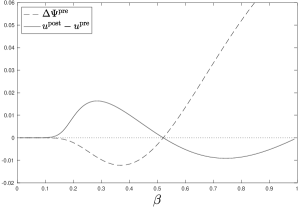
(a) Consumer Surplus of Visiting the Intermediary

(b) Combined Profits of $\mathcal{C}_{1}$ and $\mathcal{C}_{2}$

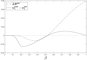
(c) Wholesale Price of Product $1$

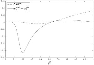
(d) Wholesale Price of Product $2$

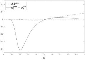
(e) Wholesale Price of Product $3$

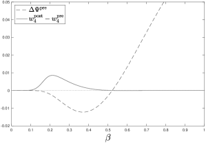
(f) Wholesale Price of Product $4$

Notes. Parameters: $n=4$, $m=3$, $\bm{\mathcal{C}}=\big{\{}\{1,2\},\{3\},\{4\}\big{\}}$ with $\mathcal{C}_{1}=\{1,2\}$, $\mathcal{C}_{2}=\{3\}$, and $\mathcal{C}_{3}=\{4\}$. $G(\xi)=1-e^{-\lambda\xi}$ with $\lambda=5$. Demands: $Q_{i}(p_{i})=\alpha_{i}(1-p_{i}(1-\sigma_{i})/(2-\sigma_{i}))^{1/(1-\sigma_{i})}$, with $\bm{\alpha}=\{1,1,1,1\}$, $\bm{\sigma}=\{0,1,1,0\}$. Marginal costs: $\bm{c}=\{\nicefrac{{1}}{{10}},\nicefrac{{1}}{{10}},\nicefrac{{1}}{{10}},\nicefrac{{1}}{{10}}\}$.

Figure 2 illustrates these results. The figure considers a setting with four products and three initial conglomerates $\bm{\mathcal{C}}=\big{\{}\{1,2\},\{3\},\{4\}\big{\}}$, where $\mathcal{C}_{1}=\{1,2\}$, $\mathcal{C}_{2}=\{3\}$, and $\mathcal{C}_{3}=\{4\}$. It then plots the value of $\Delta\Psi^{\text{pre}}$ and the effects of a merger between $\mathcal{C}_{1}$ and $\mathcal{C}_{2}$ over the surplus consumers obtain from visiting the intermediary (before shopping costs), $\mathcal{C}_{1}$’s and $\mathcal{C}_{2}$’s combined profits, and the negotiated wholesale prices.

As the figure shows, the merger leads to a higher consumer surplus, lower negotiated prices for $\mathcal{C}_{1}$’s and $\mathcal{C}_{2}$’s products, and a higher wholesale price for $\mathcal{C}_{3}$’s product when $\mathcal{C}_{1}$’s and $\mathcal{C}_{2}$’s portfolios are complements to the intermediary at the premerger prices (i.e., when $\Delta\Psi^{\text{pre}}<0$). However, these inequalities are reversed when the portfolios are seen as substitutes by the intermediary at the premerger prices (i.e., when $\Delta\Psi^{\text{pre}}>0$).

Before moving on, it is important to highlight that a merger between $\mathcal{C}_{1}$ and $\mathcal{C}_{2}$ can be profitable in this setting irrespective of whether $\Delta\Psi^{\text{pre}}\gtrless 0$. The latter is shown in panel (b) of Figure 2. However, the underlying reason the merger is profitable when $\Delta\Psi^{\text{pre}}<0$ is different than that when $\Delta\Psi^{\text{pre}}>0$.

Indeed, when $\beta$ is low enough—so suppliers’ bargaining weight is high relative to the intermediary—the double-markup problem due to linear contracts is severe. As a result, the merger can be profitable even if it weakens suppliers’ bargaining leverage (i.e., if $\Delta\Psi^{\text{pre}}<0$), as it helps suppliers commit to decreasing wholesale prices, mitigating the double-markup problem. Thus, even though $\mathcal{C}_{1}$ and $\mathcal{C}_{2}$ end up receiving a smaller fraction of the intermediary’s trade gains postmerger, the transaction increases the size of these gains.

In contrast, when $\beta$ is high enough, the double-markup problem is less severe. As a result, the merger will be profitable for $\mathcal{C}_{1}$ and $\mathcal{C}_{2}$ only if $\Delta\Psi^{\text{pre}}>0$. This is because division-of-surplus considerations now trump the size-of-trade-gains considerations. The transaction thus worsens double-marginalization but allows the merging conglomerates to appropriate a higher fraction of the intermediary’s surplus.

3.3 Portfolios can be Substitutes or Complements for Intermediaries

Let $\tilde{G}(\bm{p},\bm{\mathcal{G}})\equiv G\big{(}\sum_{\mathcal{C}_{j}\in\bm{\mathcal{G}}}\sum_{i\in\mathcal{C}_{j}}v_{i}(p_{i})\big{)}$ be the consumer traffic function given the set of agreements $\bm{\mathcal{G}}\in 2^{\bm{\mathcal{C}}}$ and the vector of retail prices $\bm{p}$. The next proposition shows that $\mathcal{C}_{1}$ and $\mathcal{C}_{2}$ can be substitutes or complements for the intermediary in profits, despite the presence of consumer-level complementarities. The proposition also shows that the first preliminary test to assess the complementarity of two portfolios for the intermediary—based on the composition of the intermediary’s lineup or the weak complementarity of the portfolios in generating traffic—remains valid here.

Proposition 4.

Premerger, the merging portfolios can be complements or substitutes for the intermediary despite the existence of complementarities at the consumer level, i.e., $\Delta\Psi^{\text{pre}}\gtrless 0$. However, if either:

• The intermediary’s lineup is comprised solely of the merging portfolios, i.e., $\bm{\mathcal{C}}\setminus\mathcal{U}=\emptyset$.

• Or if premerger the merging portfolios are complements in generating consumer traffic, i.e.,

  $$\textstyle\sum_{j=1,2}\big{(}\tilde{G}(\bm{p}^{\text{pre}},\bm{\mathcal{C}})-\tilde{G}(\bm{p}^{\text{pre}},\bm{\mathcal{C}}\setminus\mathcal{C}_{j})\big{)}\geq\tilde{G}(\bm{p}^{\text{pre}},\bm{\mathcal{C}})-\tilde{G}(\bm{p}^{\text{pre}},\bm{\mathcal{C}}\setminus\mathcal{U})$$

Then $\Delta\Psi^{\text{pre}}\leq 0$.

Proof.

First, that $\Delta\Psi^{\text{pre}}\gtrless 0$ can be immediately seen from Figure 2. The proof of points (i) and (ii), in turn, closely follows the analysis of Section 2. Fix an arbitrary $(\bm{w},\bm{p})$ and for notational simplicity, let $\Pi_{j}(\bm{p},\bm{w})\equiv\textstyle\sum_{i\in\mathcal{C}_{j}}\pi_{i}(p_{i};w_{i})$. Evaluating (9) in the definition of $\Delta\Psi$ given by (15) and rearranging terms leads to:

$$\textstyle\Delta\Psi=\left(\sum_{k\in(\bm{\mathcal{C}}\setminus\mathcal{U})}\Pi_{k}(\bm{p},\bm{w})\right)\big{[}\tilde{G}(\bm{p},\bm{\mathcal{C}})-\tilde{G}(\bm{p},\bm{\mathcal{C}}\setminus\mathcal{U})-\textstyle\sum_{j=1,2}\big{(}\tilde{G}(\bm{p},\bm{\mathcal{C}})-\tilde{G}(\bm{p},\bm{\mathcal{C}}\setminus\mathcal{C}_{j})\big{)}\big{]}\\ -\Pi_{1}(\bm{p},\bm{w})\big{[}\tilde{G}(\bm{p},\bm{\mathcal{C}})-\tilde{G}(\bm{p},\bm{\mathcal{C}}\setminus\mathcal{C}_{2})\big{]}-\Pi_{2}(\bm{p},\bm{w})\big{[}\tilde{G}(\bm{p},\bm{\mathcal{C}})-\tilde{G}(\bm{p},\bm{\mathcal{C}}\setminus\mathcal{C}_{1})\big{]}$$ (16)

Since the second and the third terms on the right-hand side of (16) are weakly negative, it is clear that $\Delta\Psi\leq 0$ if either $\bm{\mathcal{C}}\setminus\mathcal{U}=\emptyset$ (since then $\sum_{k\in(\bm{\mathcal{C}}\setminus\mathcal{U})}\Pi_{k}(\bm{p},\bm{w})=0$) or if:

$$\textstyle\sum_{j=1,2}\big{(}\tilde{G}(\bm{p},\bm{\mathcal{C}})-\tilde{G}(\bm{p},\bm{\mathcal{C}}\setminus\mathcal{C}_{j})\big{)}\geq\tilde{G}(\bm{p},\bm{\mathcal{C}})-\tilde{G}(\bm{p},\bm{\mathcal{C}}\setminus\mathcal{U})$$

Since the above results hold for an arbitrary $(\bm{w},\bm{p})$, they hold when $(\bm{w},\bm{p})=(\bm{w}^{\text{pre}},\bm{p}^{\text{pre}})$.∎

I now show that the additional screening test—based on the role played by the merging portfolios in the intermediary’s lineup—also holds in this setting. I also elaborate on the divestiture measures proposed in Section 2.4. As a first step, let me begin by defining the concept of a pure profit contributor and a pure traffic generator in the current setting:

Definition.

Product $i$ is said to be a pure (premerger) profit contributor if $v_{i}(p_{i}^{\text{pre}})=0$ and $\pi_{i}(p_{i}^{\text{pre}};w_{i}^{\text{pre}})>0$, while it is said to be a pure (premerger) traffic generator if $v_{i}(p_{i}^{\text{pre}})>0$ and $\pi_{i}(p_{i}^{\text{pre}};w_{i}^{\text{pre}})=0$.

With these definitions at hand, I can then extend Proposition 3 of Section 2:

Proposition 5.

Suppose that $\bm{\mathcal{C}}\setminus\mathcal{U}\neq\emptyset$, and that for any given $\bm{p}$, $\tilde{G}(\bm{p},\bm{\mathcal{G}})$ is submodular in $\bm{\mathcal{G}}$. Then:

• If $\mathcal{C}_{1}$’s portfolio solely comprises pure (premerger) profit contributors and $\mathcal{C}_{2}$’s portfolio solely comprises pure (premerger) traffic generators (or vice versa), then $\Delta\Psi^{\text{pre}}<0$.

• If both $\mathcal{C}_{1}$’s and $\mathcal{C}_{2}$’s portfolios are comprised solely of pure (premerger) traffic generators, then $\Delta\Psi^{\text{pre}}>0$.

Proof.

This proof is almost identical to that of Proposition 3. For an arbitrary $(\bm{w},\bm{p})$, let $\Pi_{j}(\bm{p},\bm{w})\equiv\textstyle\sum_{i\in\mathcal{C}_{j}}\pi_{i}(p_{i};w_{i})$ and $V_{j}(\bm{p},\bm{w})\equiv\textstyle\sum_{i\in\mathcal{C}_{j}}v_{i}(p_{i})$. Note then that $\Delta\Psi$ can be written as:

$$\Delta\Psi\equiv\textstyle\left(\sum_{k\in(\bm{\mathcal{C}}\setminus\mathcal{U})}\Pi_{k}(\bm{p},\bm{w})\right)\big{[}\tilde{G}(\bm{p},\bm{\mathcal{C}})-\tilde{G}(\bm{p},\bm{\mathcal{C}}\setminus\mathcal{U})-\textstyle\sum_{j=1,2}\big{(}\tilde{G}(\bm{p},\bm{\mathcal{C}})-\tilde{G}(\bm{p},\bm{\mathcal{C}}\setminus\mathcal{C}_{j})\big{)}\big{]}\\ -\Pi_{1}(\bm{p},\bm{w})\big{[}\tilde{G}(\bm{p},\bm{\mathcal{C}})-\tilde{G}(\bm{p},\bm{\mathcal{C}}\setminus\mathcal{C}_{2})\big{]}-\Pi_{2}(\bm{p},\bm{w})\big{[}\tilde{G}(\bm{p},\bm{\mathcal{C}})-\tilde{G}(\bm{p},\bm{\mathcal{C}}\setminus\mathcal{C}_{1})\big{]}$$

If $\mathcal{C}_{1}$’s portfolio solely comprises pure (premerger) profit contributors and $\mathcal{C}_{2}$’s portfolio comprises solely pure (premerger) traffic generators, then $\Pi_{1}(\bm{p}^{\text{pre}},\bm{w}^{\text{pre}})>0$, $V_{1}(\bm{p}^{\text{pre}})=0$, $\Pi_{2}(\bm{p}^{\text{pre}},\bm{w}^{\text{pre}})=0$, and $V_{2}(\bm{p}^{\text{pre}})>0$. Thus, $\tilde{G}(\bm{p}^{\text{pre}},\bm{\mathcal{C}})>\tilde{G}(\bm{p}^{\text{pre}},\bm{\mathcal{C}}\setminus\mathcal{C}_{2})$, $\tilde{G}(\bm{p}^{\text{pre}},\bm{\mathcal{C}})=\tilde{G}(\bm{p}^{\text{pre}},\bm{\mathcal{C}}\setminus\mathcal{C}_{1})$, and:

$$\tilde{G}(\bm{p}^{\text{pre}},\bm{\mathcal{C}})-\tilde{G}(\bm{p}^{\text{pre}},\bm{\mathcal{C}}\setminus\mathcal{U})-\textstyle\sum_{j=1,2}\big{(}\tilde{G}(\bm{p}^{\text{pre}},\bm{\mathcal{C}})-\tilde{G}(\bm{p}^{\text{pre}},\bm{\mathcal{C}}\setminus\mathcal{C}_{j})\big{)}=0$$

Therefore, $\Delta\Psi^{\text{pre}}=-\Pi_{1}(\bm{p}^{\text{pre}},\bm{w}^{\text{pre}})\big{[}\tilde{G}(\bm{p}^{\text{pre}},\bm{\mathcal{C}})-\tilde{G}(\bm{p}^{\text{pre}},\bm{\mathcal{C}}\setminus\mathcal{C}_{2})\big{]}<0$.

On the other hand, if both $\mathcal{C}_{1}$’s and $\mathcal{C}_{2}$’s portfolios solely comprise pure (premerger) traffic generators, then $\Pi_{1}(\bm{p}^{\text{pre}},\bm{w}^{\text{pre}})=\Pi_{2}(\bm{p}^{\text{pre}},\bm{w}^{\text{pre}})=0$, $V_{1}(\bm{p}^{\text{pre}})>0$, and $V_{2}(\bm{p}^{\text{pre}})>0$. Thus,

$$\Delta\Psi^{\text{pre}}=\textstyle\left(\sum_{k\in(\bm{\mathcal{C}}\setminus\mathcal{U})}\Pi_{k}(\bm{p}^{\text{pre}},\bm{w}^{\text{pre}})\right)\\ \times\big{[}\tilde{G}(\bm{p}^{\text{pre}},\bm{\mathcal{C}})-\tilde{G}(\bm{p}^{\text{pre}},\bm{\mathcal{C}}\setminus\mathcal{U})-\textstyle\sum_{j=1,2}\big{(}\tilde{G}(\bm{p}^{\text{pre}},\bm{\mathcal{C}})-\tilde{G}(\bm{p}^{\text{pre}},\bm{\mathcal{C}}\setminus\mathcal{C}_{j})\big{)}\big{]}$$

Hence, $\Delta\Psi^{\text{pre}}\geq 0$ as $\bm{\mathcal{C}}\setminus\mathcal{U}\neq\emptyset$, and $\tilde{G}(\bm{p},\mathcal{G})$ is submodular in the products carried by the intermediary for any given $\bm{p}$ (in particular, when $\bm{p}=\bm{p}^{\text{pre}}$). ∎

The intuition for Proposition 5 is the same as that for Proposition 3: the complementarity in profits is maximized, and the substitutability of traffic is minimized by combining a pure profit contributor and a pure traffic generator portfolio. In contrast, the complementarity in profits is minimized, and traffic substitutability is maximized by combining two pure traffic generators.

As I stated in Section 2, no product will ever be a pure profit contributor or a pure traffic generator. However, just as in the case of Proposition 3, the results of Proposition 5 extend beyond the limit cases considered in the proposition. The latter is illustrated in Figure 3, which depicts a situation with four products and three conglomerates premerger $\bm{\mathcal{C}}=\big{\{}\{1,2\},\{3\},\{4\}\big{\}}$.

Figure 3: The Consumer Welfare Implications of Two Different Mergers

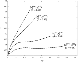
(a) Products’ Positions as $\beta$ Changes

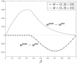
(b) Change in Consumer Welfare

Notes. Panel (a) depicts the premerger location of the four products in the $(\pi,v)$ space as a function of $\beta$. The arrows indicate how the location of a product moves as $\beta$ decreases, starting from $\beta=0.99$. Panel (b) plots the consumer welfare implications of two different potential mergers: $\mathcal{U}=\{1,2\}\cup\{3\}$ and $\mathcal{U}=\{1,2\}\cup\{4\}$. Parameters: $n=4$, $m=3$, $\bm{\mathcal{C}}=\big{\{}\{1,2\},\{3\},\{4\}\big{\}}$. $G(\xi)=1-e^{-\lambda\xi}$ with $\lambda=5$. Demands: $Q_{i}(p_{i})=\alpha_{i}(1-p_{i}(1-\sigma_{i})/(2-\sigma_{i}))^{1/(1-\sigma_{i})}$, with $\bm{\alpha}=\{1,1,1,1\}$ and $\bm{\sigma}=\{1,-1,\nicefrac{{3}}{{2}},-6\}$. Marginal costs: $\bm{c}=\{\nicefrac{{1}}{{10}},\nicefrac{{1}}{{10}},\nicefrac{{1}}{{10}},\nicefrac{{1}}{{10}}\}$.

More precisely, panel (a) of that figure depicts the premerger location of the four products in the $(\pi,v)$ space as a function of $\beta$. These locations now change depending on the value of $\beta$ since they are endogenous equilibrium objects. The arrows indicate how the location of a product moves as $\beta$ decreases, starting from $\beta=0.99$. Panel (b), in turn, plots the consumer welfare implications of two different potential mergers, $\mathcal{U}=\{1,2\}\cup\{3\}$ and $\mathcal{U}=\{1,2\}\cup\{4\}$

As the figure shows, when conglomerate $\mathcal{C}_{1}=\{1,2\}$ acquires product $3$—which was contributing to the intermediary’s profits mainly via traffic in the premerger scenario—the merger leads to a reduction in consumer welfare. In contrast, the transaction unambiguously increases consumer surplus when the conglomerate acquires product $4$ instead—a product that contributed to the intermediary mainly through direct profits before the merger.

As noted in Section 2, Propositions 4 and 5 also lead to novel divestiture measures. Indeed, they suggest that to mitigate the potential adverse effect of the merger, authorities should aim to force the merging entities to divest those products located (premerger) in the northwest corner of the $(\pi,v)$ space. The idea is to minimize any potential substitutability of traffic between the merging portfolios while keeping direct profit complementarities intact.

This last point is illustrated in Figure 4(a), which builds upon Figure 3. The figure depicts the consumer welfare implications of forcing conglomerate $\mathcal{C}_{1}=\{1,2\}$ to divest product $1$ as a precondition to acquiring product $3$, comparing it to the case in which no remedy is imposed. As the figure shows, the divestiture remedy almost completely offsets the negative impact of the original transaction.

Unfortunately, however, just as in the simple model of Section 2, forcing the merging entities to divest the wrong products can backfire. Figure 4(b) shows an example of this phenomenon, depicting the implications of forcing conglomerate $\mathcal{C}_{1}=\{1,2\}$ to divest product $2$ instead of product $1$ as a precondition to acquiring product $3$.

Figure 4: The Consumer Welfare Implications of Two Different Divestiture Measures

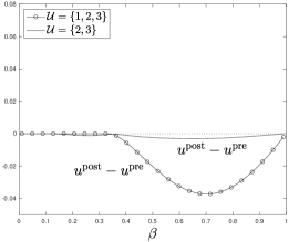
(a) Divesting Product $1$

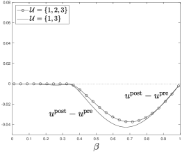
(b) Divesting Product $2$

Notes. Parameters: $n=4$, $m=3$, $\bm{\mathcal{C}}=\big{\{}\{1,2\},\{3\},\{4\}\big{\}}$. $G(\xi)=1-e^{-\lambda\xi}$ with $\lambda=5$. Demands: $Q_{i}(p_{i})=\alpha_{i}(1-p_{i}(1-\sigma_{i})/(2-\sigma_{i}))^{1/(1-\sigma_{i})}$, with $\bm{\alpha}=\{1,1,1,1\}$ and $\bm{\sigma}=\{1,-1,\nicefrac{{3}}{{2}},-6\}$. Marginal costs: $\bm{c}=\{\nicefrac{{1}}{{10}},\nicefrac{{1}}{{10}},\nicefrac{{1}}{{10}},\nicefrac{{1}}{{10}}\}$.

As I mentioned in Section 2.3, products with “more concave” and “rectangular-shaped” demands will have a higher $\pi_{i}^{\textrm{pre}}/v_{i}^{\textrm{pre}}$ ratio. This was because the intermediary can extract a larger share of consumer surplus without introducing significant monopoly distortions the more concave and rectangular-shaped a product’s demand is, leading to a higher $\pi_{i}^{\textrm{pre}}/v_{i}^{\textrm{pre}}$.

Figure 5: Curvature of Demand and Products’ Premerger $(\pi,v)$

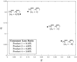
(a) Premerger $(\pi,v)$ Distribution (when $\beta=0.6$)

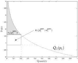
(b) Product $1$ ($\sigma_{1}=1$)

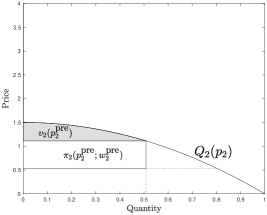
(c) Product $2$ ($\sigma_{2}=-1$)

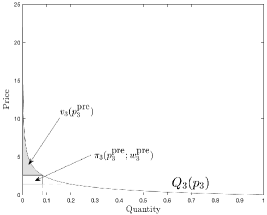
(d) Product $3$ ($\sigma_{3}=\nicefrac{{3}}{{2}}$)

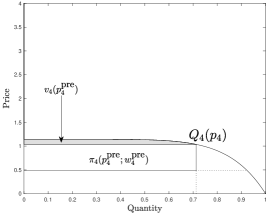
(e) Product $4$ ($\sigma_{4}=-6$)

Notes. Parameters: $n=4$, $m=3$, $\beta=0.6$, $\bm{\mathcal{C}}=\big{\{}\{1,2\},\{3\},\{4\}\big{\}}$. $G(\xi)=1-e^{-\lambda\xi}$ with $\lambda=5$. Demands: $Q_{i}(p_{i})=\alpha_{i}(1-p_{i}(1-\sigma_{i})/(2-\sigma_{i}))^{1/(1-\sigma_{i})}$, with $\bm{\alpha}=\{1,1,1,1\}$, $\bm{\sigma}=\{1,-1,\nicefrac{{3}}{{2}},-6\}$. Marginal costs: $\bm{c}=\{\nicefrac{{1}}{{10}},\nicefrac{{1}}{{10}},\nicefrac{{1}}{{10}},\nicefrac{{1}}{{10}}\}$. Equilibrium outcome: $\bm{w}^{\text{pre}}=\{0.87,0.53,3.85,0.48\}$ and $\bm{p}^{\text{pre}}=\{1.57,1.10,6.47,1.03\}$.

This intuition is illustrated in Figure 5, which depicts the premerger scenario underlying Figures 3 and 4 when $\beta=0.6$. In this particular example, consumers’ demands belong to the family of constant-passthrough demands first introduced by Bulow and Pfleiderer (1983):

$$Q_{i}(p_{i})=\alpha_{i}\left[1-\left(\frac{1-\sigma_{i}}{2-\sigma_{i}}\right)p_{i}\right]^{\frac{1}{1-\sigma_{i}}}\ \ \text{where $\alpha_{i}\in(0,\infty)$ and $\sigma_{i}\in(-\infty,2)$}$$

This is a relatively general family of demand functions that has as special cases (i) the unit (or perfectly inelastic) demand ($\sigma_{i}\to-\infty$), (ii) linear demand ($\sigma_{i}=0$), and (iii) constant markup demand ($\sigma_{i}\to 1$), among others. The parameter $\alpha_{i}$ captures the scale of the demand, while the parameter $\sigma_{i}$ captures its curvature. More precisely, $Q_{i}(p_{i})$ will be concave when $\sigma_{i}<0$, linear when $\sigma_{i}=0$, and convex when $\sigma_{i}>0$.

As the figure shows, products with “more concave” and “rectangular-shaped” demands—such as products $2$ and $4$—have a higher $\pi_{i}^{\textrm{pre}}/v_{i}^{\textrm{pre}}$ ratio as they are used by the intermediary to mainly generate direct profits. Conversely, products with “more convex” demands—such as products $1$ and $3$—have a lower $\pi_{i}^{\textrm{pre}}/v_{i}^{\textrm{pre}}$ ratio, as the intermediary uses those products to generate traffic.

4 Final Remarks

The effects of cross-market mergers of upstream suppliers in the presence of common customers have been very controversial. Some researchers have argued that common customers make products substitutes for intermediaries; thus, such mergers likely increase negotiated prices. Other researchers posit that because products are complements to customers, they must also be complements for intermediaries. Hence, these types of transactions should lead to lower, not higher, negotiated prices.

In this paper, I contribute to this debate by showing that two products can be complements for customers but substitutes for the intermediary in terms of profits. This seemingly contradictory result arises when two products serve a similar role in attracting consumers to purchase the bundle and are, thus, substitutes in generating consumer traffic for other products in the intermediary’s lineup.

This result leads to novel antitrust recommendations. First, it suggests a first-pass test to assess whether the portfolios of two merging suppliers will be complements in profits for the intermediary. Second, it implies that authorities can assess the likelihood of harm in a particular transaction by assessing the role played by the merging products in the intermediary’s lineup. Finally, the aforementioned result leads to a new divestiture framework for these types of transactions: to offset the potential negative effects of a merger, authorities should focus their divestiture efforts on the products that contribute to the intermediaries’ overall profits primarily via consumer traffic.

Appendix

Appendix A Supermodularity of $U(\mathcal{G};\xi)$

Instead of directly showing that $U(\mathcal{G};\xi)=\max\{\sum_{i\in\mathcal{G}}v_{i}-\xi,0\}$ is a supermodular set function (which requires going over all subsets of $2^{\{\emptyset,0,1,2\}}$), I will use the following theorem due to Topkis (1978) and reproduced in Brynjolfsson and Milgrom (2013, Theorem 1b., p.19):

Theorem A.0.1.

Suppose that $f:S\to\mathbb{R}$, where $S$ is a product set $S=\times_{i=1}^{n}S_{i}$, and each $S_{i}\subseteq\mathbb{R}$. Then $f$ is supermodular if and only if for all $1\leq i<j\leq n$ and all $x\in S$, the function $g(z_{i},z_{j})\equiv f(z_{i},z_{j},x_{-ij})$ is supermodular.

To use this theorem, note that there is a one-to-one mapping between $U(\mathcal{G};\xi)$ and the function $\tilde{U}:\{0,1\}^{3}\to\mathbb{R}$ defined as $\tilde{U}(x_{i},x_{j},x_{k};\xi)=\max\{x_{i}v_{i}+x_{j}v_{j}+x_{k}v_{k}-\xi,0\}$ (intuitively, $x_{i}\in\{0,1\}$ denotes whether the intermediary stocks product $i$). Thus—and given that $\tilde{U}(x_{i},x_{j},x_{k};\xi)$ is symmetric upon permutations of $(x_{i},x_{j},x_{k})$—the indirect utility function will be supermodular in the set of products if and only if for all $x_{k}\in\{0,1\}$ the following condition holds:

$$\tilde{U}(1,1,x_{k};\xi)+\tilde{U}(0,0,x_{k};\xi)-\tilde{U}(1,0,x_{k};\xi)-\tilde{U}(0,1,x_{k};\xi)\geq 0$$ (17)

To show the latter, denote by $\delta$ the left-hand side of (17) and suppose, without loss of generality, that $v_{i}\geq v_{j}$. Then:

• If $x_{k}v_{k}\geq\xi$, then $\delta=0.$

• If $v_{j}+x_{k}v_{k}\geq\xi>x_{k}v_{k}$, then $\delta=\xi-x_{k}v_{k}>0$.

• If $v_{i}+x_{k}v_{k}\geq\xi>v_{j}+x_{k}v_{k}$, then $\delta=v_{j}\geq 0$.

• If $v_{i}+v_{j}+x_{k}v_{k}\geq\xi>v_{i}+x_{k}v_{k}$, then $\delta=v_{i}+v_{j}+x_{k}v_{k}-\xi\geq 0$.

• If $\xi>v_{i}+v_{j}+x_{k}v_{k}$, then $\delta=0$.

Thus, $\delta\geq 0$ always (with strict inequality in some circumstances); therefore, the indirect utility function of a consumer with a shopping cost $\xi$ is supermodular in the set of products. $\square$

Appendix B Divestiture Measures with Four Products

In this appendix, I derive the equilibrium negotiated payments under four scenarios: premerger, postmerger with no divestiture, postmerger with the divestiture of product $1$, and postmerger with the divestiture of product $2$. Then, I obtain the expressions for $\Delta T(\text{no divestiture})$, $\Delta T(\text{divest}\ 1)$, and $\Delta T(\text{divest}\ 2)$, as stated in Section 2.4 of the main text.

Premerger Equilibrium.— Consider first the premerger equilibrium. Following a logic analogous to that used in Section 2.2, the equilibrium negotiated payments are $t_{i}^{\text{pre}}=\big{(}\Psi(\mathcal{N})-\Psi(\mathcal{N}\setminus\{i\})-\Phi_{i}\big{)}\big{/}2$ for $i=0,3$, and $\textstyle\sum_{i=1,2}t_{i}^{\text{pre}}=\big{(}\Psi(\mathcal{N})-\Psi(\mathcal{N}\setminus\{1,2\})-\sum_{i=1,2}\Phi_{i}\big{)}\big{/}2$ for $i\in\mathcal{U}=\{1,2\}$. Hence $T^{\text{pre}}=\big{(}2\Psi(\mathcal{N})-\Psi(\mathcal{N}\setminus\{1,2\})-\Psi(\mathcal{N}\setminus\{3\})-\sum_{i=1,2,3}\Phi_{i}\big{)}\big{/}2$.

Postmerger - No Divestiture.— Consider the postmerger equilibrium without any divestiture measures. The equilibrium negotiated payments then satisfy $t_{0}^{\text{post}}(\text{no divestiture})=\big{(}\Psi(\mathcal{N})-\Psi(\mathcal{N}\setminus\{0\})-\Phi_{i}\big{)}\big{/}2$, and $\textstyle\sum_{i=1,2,3}t_{i}^{\text{post}}(\text{no divestiture})=\big{(}\Psi(\mathcal{N})-\Psi(\mathcal{N}\setminus\{1,2,3\})-\sum_{i=1,2,3}\Phi_{i}\big{)}\big{/}2$. Thus, $T^{\text{post}}(\text{no divestiture})=\big{(}\Psi(\mathcal{N})-\Psi(\mathcal{N}\setminus\{1,2,3\})-\sum_{i=1,2,3}\Phi_{i}\big{)}\big{/}2$.

Postmerger - Divestiture of Product $1$.— Suppose that $\mathcal{U}$ must divest product $1$ to acquire product $3$. The equilibrium negotiated payments are then $t_{i}^{\text{post}}(\text{divest 1})=\big{(}\Psi(\mathcal{N})-\Psi(\mathcal{N}\setminus\{i\})-\Phi_{i}\big{)}\big{/}2$ for $i=0,1$, and $\textstyle\sum_{i=2,3}t_{i}^{\text{post}}(\text{divest 1})=\big{(}\Psi(\mathcal{N})-\Psi(\mathcal{N}\setminus\{2,3\})-\sum_{i=2,3}\Phi_{i}\big{)}/2$. Hence, $T^{\text{post}}(\text{divest 1})=\big{(}2\Psi(\mathcal{N})-\Psi(\mathcal{N}\setminus\{2,3\})-\Psi(\mathcal{N}\setminus\{2\})-\sum_{i=1,2,3}\Phi_{i}\big{)}\big{/}2$.

Postmerger - Divestiture of Product $2$.— Finally, suppose that $\mathcal{U}$ must divest product $2$ to acquire product $3$. The equilibrium negotiated payments are then $t_{i}^{\text{post}}(\text{divest 2})=\big{(}\Psi(\mathcal{N})-\Psi(\mathcal{N}\setminus\{i\})-\Phi_{i}\big{)}\big{/}2$ for $i=0,2$, and $\textstyle\sum_{i=1,3}t_{i}^{\text{post}}(\text{divest 2})=\big{(}\Psi(\mathcal{N})-\Psi(\mathcal{N}\setminus\{1,3\})-\sum_{i=1,3}\Phi_{i}\big{)}/2$. Consequently, $T^{\text{post}}(\text{divest 2})=\big{(}2\Psi(\mathcal{N})-\Psi(\mathcal{N}\setminus\{1,3\})-\Psi(\mathcal{N}\setminus\{2\})-\sum_{i=1,2,3}\Phi_{i}\big{)}\big{/}2$.

Expressions for $\Delta T(\text{no divestiture})$, $\Delta T(\text{divest}\ 1)$, and $\Delta T(\text{divest}\ 2)$.— Combining the above results, I then have that:

$$\textstyle\Delta T(\text{no divestiture})=\big{(}\Psi(\mathcal{N}\setminus\{1,2\})+\Psi(\mathcal{N}\setminus\{3\})-\Psi(\mathcal{N})-\Psi(\mathcal{N}\setminus\{1,2,3\})\big{)}\big{/}2$$

$$\textstyle\Delta T(\text{divest}\ 1)=\big{(}\Psi(\mathcal{N}\setminus\{1,2\})+\Psi(\mathcal{N}\setminus\{3\})-\Psi(\mathcal{N}\setminus\{1\})-\Psi(\mathcal{N}\setminus\{2,3\})\big{)}\big{/}2$$

$$\textstyle\Delta T(\text{divest}\ 2)=\big{(}\Psi(\mathcal{N}\setminus\{1,2\})+\Psi(\mathcal{N}\setminus\{3\})-\Psi(\mathcal{N}\setminus\{2\})-\Psi(\mathcal{N}\setminus\{1,3\})\big{)}\big{/}2$$

References

- (1)
- Baye, von Schlippenbach and Wey (2018) Baye, Irina, Vanessa von Schlippenbach, and Christian Wey. 2018. “One-Stop Shopping Behavior, Buyer Power and Upstream Merger Incentives.” Journal of Industrial Economics, 66(1): 66–94.
- Brand and Rosenbaum (2019) Brand, Keith, and Ted Rosenbaum. 2019. “A Review of the Economic Literature on Cross-Market Health Care Mergers.” Antitrust Law Journal, 82: 533–549.
- Brynjolfsson and Milgrom (2013) Brynjolfsson, Erik, and Paul Milgrom. 2013. “Chapter 1: Complementarity in Organizations.” In . Vol. 1 of Handbook of Organizational Economics, 11–55. Princeton University Press.
- Bulow and Pfleiderer (1983) Bulow, Jeremy I., and Paul Pfleiderer. 1983. “A Note on the Effect of Cost Changes on Prices.” Journal of Political Economy, 91(1): 182–185.
- Chambolle and Molina (2023) Chambolle, Claire, and Hugo Molina. 2023. “A Buyer Power Theory of Exclusive Dealing and Exclusionary Bundling.” American Economic Journal: Microeconomics, Forthcoming.
- Collard-Wexler, Gowrisankaran and Lee (2019) Collard-Wexler, Allan, Gautam Gowrisankaran, and Robin S. Lee. 2019. ““Nash-in-Nash” Bargaining: A Microfoundation for Applied Work.” Journal of Political Economy, 127(1): 163–195.
- Crawford and Yurukoglu (2012) Crawford, Gregory S., and Ali Yurukoglu. 2012. “The Welfare Effects of Bundling in Multichannel Television Markets.” American Economic Review, 102(2): 643–85.
- Crawford et al. (2018) Crawford, Gregory S., Robin S. Lee, Michael D. Whinston, and Ali Yurukoglu. 2018. “The Welfare Effects of Vertical Integration in Multichannel Television Markets.” Econometrica, 86(3): 891–954.
- Dafny, Ho and Lee (2019) Dafny, Leemore, Kate Ho, and Robin S. Lee. 2019. “The Price Effects of Cross-Market Mergers: Theory and Evidence from the Hospital Industry.” The RAND Journal of Economics, 50(2): 286–325.
- Dobson and Waterson (1997) Dobson, Paul W., and Michael Waterson. 1997. “Countervailing Power and Consumer Prices.” The Economic Journal, 107(441): 418–430.
- Easterbrook et al. (2018) Easterbrook, Kathleen, Gautam Gowrisankaran, Dina Older Aguilar, and Yufei Wu. 2018. “Accounting for Complementarities in Hospital Mergers: Is a Substitute Needed for Current Approaches?” Antitrust Law Journal, 82: 497.
- European Commission (2008) European Commission. 2008. “Guidelines on the Assessment of Non-Horizontal Mergers under the Council Regulation on the Control of Concentrations between Undertakings.” Official Journal of the European Union, 51: 6–25.
- Farrell et al. (2011) Farrell, Joseph, David J. Balan, Keith Brand, and Brett W. Wendling. 2011. “Economics at the FTC: Hospital Mergers, Authorized Generic Drugs, and Consumer Credit Markets.” Review of Industrial Organization, 39: 271–296.
- Gowrisankaran, Nevo and Town (2015) Gowrisankaran, Gautam, Aviv Nevo, and Robert Town. 2015. “Mergers When Prices Are Negotiated: Evidence from the Hospital Industry.” American Economic Review, 105(1): 172–203.
- Greenlee, Reitman and Sibley (2008) Greenlee, Patrick, David Reitman, and David S. Sibley. 2008. “An Antitrust Analysis of Bundled Loyalty Discounts.” International Journal of Industrial Organization, 26(5): 1132–1152.
- Ho and Lee (2017) Ho, Kate, and Robin S. Lee. 2017. “Insurer Competition in Health Care Markets.” Econometrica, 85(2): 379–417.
- Ho and Lee (2019) Ho, Kate, and Robin S. Lee. 2019. “Equilibrium Provider Networks: Bargaining and Exclusion in Health Care Markets.” American Economic Review, 109(2): 473–522.
- Horn and Wolinsky (1988) Horn, Henrick, and Asher Wolinsky. 1988. “Bilateral Monopolies and Incentives for Merger.” RAND Journal of Economics, 19(3): 408–419.
- Ide and Montero (2023) Ide, Enrique, and Juan-Pablo Montero. 2023. “Monopolization with Must-Haves.” Working Paper.
- Lewis and Pflum (2015) Lewis, Matthew S., and Kevin E. Pflum. 2015. “Diagnosing Hospital System Bargaining Power in Managed Care Networks.” American Economic Journal: Economic Policy, 7(1): 243–74.
- Luco and Marshall (2020) Luco, Fernando, and Guillermo Marshall. 2020. “The Competitive Impact of Vertical Integration by Multiproduct Firms.” American Economic Review, 110(7): 2041–64.
- Nevo (2014) Nevo, Aviv. 2014. “Mergers that Increase Bargaining Leverage.” Remarks as Prepared for the Stanford Institute for Economic Policy Research and Cornerstone Research Conference on Antitrust in Highly Innovative Industries. https://www.justice.gov/atr/file/517781/download [Accessed: December 19, 2022].
- Peters (2014) Peters, Craig T. 2014. “Bargaining Power and the Effects of Joint Negotiation: The ‘Recapture Effect’.” DOJ Discussion Paper EAG 14-3.
- Rhodes, Watanabe and Zhou (2021) Rhodes, Andrew, Makoto Watanabe, and Jidong Zhou. 2021. “Multiproduct Intermediaries.” Journal of Political Economy, 129(2): 421–464.
- Rogerson (2020) Rogerson, William P. 2020. “Modelling and Predicting the Competitive Effects of Vertical Mergers: The Bargaining Leverage over Rivals Effect.” Canadian Journal of Economics/Revue canadienne d’économique, 53(2): 407–436.
- Shapiro (2018) Shapiro, Carl. 2018. “Expert Report. United States of America v. AT&T Inc., DirecTV Group Holdings, LLC, and Time Warner Inc., Case. No. 1:17-cv-02511 (RJL). https://www.justice.gov/atr/case-document/file/1081336/download [Accessed: December 19, 2022].”
- Stole and Zwiebel (1996) Stole, Lars A., and Jeffrey Zwiebel. 1996. “Intra-Firm Bargaining under Non-Binding Contracts.” The Review of Economic Studies, 63(3): 375–410.
- Topkis (1978) Topkis, Donald M. 1978. “Minimizing a Submodular Function on a Lattice.” Operations Research, 26(2): 305–321.
- Vistnes and Sarafidis (2013) Vistnes, Gregory S., and Yianis Sarafidis. 2013. “Cross-Market Hospital Mergers: A Holistic Approach.” Antitrust Law Journal, 79(1): 253–293.
- Whinston (1990) Whinston, Michael D. 1990. “Tying, Foreclosure and Exclusion.” American Economic Review, 80(4): 837–859.