Solving fluid flow problems in space-time with multiscale stabilization: formulation and examples

Abstract

We solve fluid flow problems through a space-time finite element method. The weak form of the Navier-Stokes equations is stabilized using the variational multi-scale formulation. The finite element problem is posed on the “full” space-time domain, considering time as another dimension. We apply this method on two benchmark problems in computational fluid dynamics, namely, lid-driven cavity flow and flow past a circular cylinder. We validate the current method with existing results from literature and show that very large space-time blocks can be solved using our approach.

baskarg@iastate.eduBaskar Ganapathysubramanian

1 Introduction

Transient physical processes are typically described by time-dependent partial differential equations (PDEs). Mathematical analysis shows that, given smooth and compatible initial condition and boundary conditions, many of these equations have solutions of certain regularity in both space and time dimensions. When solving these equations numerically, the most common practice is to use the method of lines which has two variants: (i) where the PDE is discretized in space to obtain a large system of ordinary differential equations (ODEs), which are then integrated in time; and (ii) where the equations are discretized is time first, to obtain a continuous PDE in spatial variables, which are then solved using techniques for solving stationary PDEs.

The nature of the method of lines makes it a sequential process. To illustrate this, suppose $I=[0,T]$ denotes a time interval of interest. In the method of lines, say we discretize this interval into $n_{t}$ finite time steps, each of length $\Delta t=\frac{T}{(n_{t}-1)}$. So the PDE of interest, now semidiscrete, has to be solved at time points: $\Delta t,\ 2\Delta t,\ 3\Delta t,...,\ (n_{t}-1)\Delta t=T$. In such algorithms, the solution at a particular step depends on the solutions at previous time steps. Thus, the solution process essentially becomes evolutionary: marching from one time step to the next, thereby mimicking the physical process itself.

But, it is not necessary for a numerical method to really mimic the physical process in its evolutionary characteristics. Prior work [1, 2, 3, 4, 5, 6, 7] has shown that solving for a solution at a later time does not have to wait for the solutions of intermediate points to finish. Rather, all these computations can progress in parallel. A brief review of some of these methods can be found in [8]. A common theme that runs through these methods is the idea of parallelization of computation, possibly coupled with decomposing the spatiotemporal domain (i.e., the tensor product of the spatial domain and the time window) into multiple smaller subdomains.

Multiple types of decompositions have been proposed in the context of space-time parallelism. Early works such as [1, 9] or more recent works such as [7] decompose the PDE primarily in time. Such methods fall under the methods relying on temporal domain decomposition. Similary works based on waveform relaxation methods [5, 6] achieve decomposition primarily in spatial domain. Domain decomposition in both space and time was considered by [2, 4, 10], where mulitigrid approach was adopted to solve the spatiotemporal system of equations. But it was noticed that the multigrid coarsening does not work the same way in time as it would in the spatial dimension; in particular, coarsening in time may not always lead to right convergence.

In the context of finite element method (FEM), a method of lines discretization usually employs a finite difference scheme (e.g., Euler scheme), and many space-time parallel implementations rely on them [7, 11]. But works such as [12, 13] have applied discontinuous Galerkin (dG) discretization in the time dimension in tandem with continuous Galerkin (cG) approximation in space. These methods are also commonly known as “space-time finite element methods”, but these are still sequential in nature, i.e., one usually solves one “slab” of time-window before solving another in order. Some more examples of this kind of discretization, especially in the realm of flow problems, can be found in [14, 15, 16]. More recent works such as [17] consider such a dG time discretization in a non-sequential manner.

Recently, efforts have been made to apply continuous Galerkin method for time discretization [18, 19, 20, 21]. And works such as [22] explore the scalability and advantages of solving these formulations on large computing clusters. Most of these works are limited to linear parabolic equations such as the heat equation, but they do highlight some of the issues of approximating the dependence of the solution on time through continuous basis functions, in particular, the need for a stabilized method. Theoretical analysis [23] of this problem also refers to a need for such a method.

In this work, our goal is to develop a fast and scalable continuous Galerkin method for a space-time coupled discretization of the Navier-Stokes equations. As will be discussed in Sec. 2, the stabilization requirements for the space-time discretization of the Navier-Stokes equations reduce to the following: (i) stabilization of the dominant convection terms and (ii) stabilization of the saddle point nature of the incompressible Navier-Stokes equations. The first kind of stability can be provided by multiple ways, including the streamline upwind Petrov Galerkin (SUPG) method [24], the Galerkin Least Square (GLS) method [25, 26], or the variational multiscale (VMS) method [27]. The second type of stability can be provided by the pressure stabilized Petrov Galerkin (PSPG) method [28]. But it has been shown that the application of the multiscale ideas can naturally lead to a stabilization scheme that encompass both SUPG and PSPG type of stabilizations [29]. The application of VMS also leads to a grad-divergence stabilization.

In this paper, we argue that VMS also helps stabilize the space-time variational equations in a continuous Galerkin setting. The variational problem then can be solved in a domain-decomposed manner to obtain a fully coupled space-time problem that also translates into a stable linear algebra problem. Our contributions in this paper are as follows:

1. A continuous Galerkin method for solving the Navier-Stokes equations in space-time in a non-sequential manner.

2. An application of VMS to stabilize the linear algebra problem against both spatial and temporal convective effects as well as against using equal-order velocity-pressure pair spaces.

3. A rigorous analysis of the space-time variational problem.

4. Validation of the method against benchmark problems.

The rest of the paper is organized as follows: Section 2 presents the mathematical background and derives the variational formulation, Section 3 provides an analysis of the variational problem, Section 4 provides the implementations details, Section 5 presents the numerical experiments and validation results; and Section 6 provides some discussions and conclusions.

2 Space-time variational formulation

2.1 Preliminaries

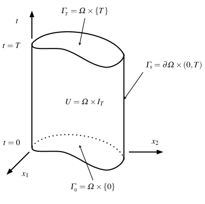
Figure 1: Schematic depiction of the space-time domain $U=\Omega\times I_{T}$, where $\Omega\subset\mathbb{R}^{d}$, and $I_{T}=[0,T]\subset\mathbb{R}^{+}.$

Consider a bounded, open spatial domain $\Omega\in\mathbb{R}^{d},d\in\{2,3\}$ with Lipschitz continuous boundary $\partial\Omega$ and a bounded time interval $I_{T}=(0,T]\in\mathbb{R^{+}}$. We define the space-time domain as the Cartesian product of the two: $U=\Omega\times I_{T}=\Omega\times(0,T]$ (see Figure 1). Suppose ${\mathbold{x}}\in\Omega$ and $t\in I_{T}$ and define $\tilde{{\mathbold{x}}}=({\mathbold{x}},t)^{T}\in U$. The overall boundary of this space-time domain is defined as $\Gamma=\partial U$. This “overall boundary” is the union of the “spatial boundaries” and the “time boundaries”. The spatial domain boundary is denoted by $\Gamma_{S}=\partial\Omega\times(0,T)$; whereas the time boundaries are denoted by $\Gamma_{0}=\bar{\Omega}\times\{0\}$ and $\Gamma_{T}=\bar{\Omega}\times\{T\}$ which are the initial and final time boundaries respectively. Therefore $\Gamma=\Gamma_{S}\cup\Gamma_{0}\cup\Gamma_{T}$.

On this space-time domain $U$, the incompressible Navier-Stokes equations can then be written for the vector function ${\mathbold{u}}={\mathbold{u}}(\tilde{{\mathbold{x}}}):U\rightarrow\mathbb{R}^{d}$ and the scalar function $p=p(\tilde{{\mathbold{x}}}):U\rightarrow\mathbb{R}$ as:

$$\frac{\partial{\mathbold{u}}}{\partial t}+({\mathbold{u}}\cdot{\mathbold{{\nabla}}}){\mathbold{u}}+\frac{1}{2}({\mathbold{{\nabla}}}\cdot{\mathbold{u}}){\mathbold{u}}-\nu\Delta{\mathbold{u}}+{\mathbold{{\nabla}}}p-{\mathbold{f}} =\mathbf{0},\text{ }\tilde{{\mathbold{x}}}\in U,$$ (1a)

$${\mathbold{{\nabla}}}\cdot{\mathbold{u}} =0,\text{ }\tilde{{\mathbold{x}}}\in U,$$ (1b)

$${\mathbold{u}} ={\mathbold{u}}_{D},\text{ }\tilde{{\mathbold{x}}}\in\Gamma_{S},$$ (1c)

$${\mathbold{u}} ={\mathbold{u}}_{0},\text{ }\tilde{{\mathbold{x}}}\in\Gamma_{0},$$ (1d)

where, ${\mathbold{u}}=(u_{1},\ldots,u_{d})^{T}$ is the velocity vector, $p$ is the pressure, and $\nu$ is the kinematic viscosity, which is assumed constant. The Reynolds number is expressed as $Re=\nicefrac{{1}}{{\nu}}$ and the forcing function ${\mathbold{f}}:U\rightarrow\mathbb{R}^{d}$ is assumed to be smooth. Note that ${\mathbold{{\nabla}}}$ is the usual spatial gradient operator in the space $\mathbb{R}^{d}$, i.e., ${\mathbold{{\nabla}}}\equiv(\nicefrac{{\partial}}{{\partial x}},\nicefrac{{\partial}}{{\partial y}})$ for $d=2$ and ${\mathbold{{\nabla}}}\equiv(\nicefrac{{\partial}}{{\partial x}},\nicefrac{{\partial}}{{\partial y}},\nicefrac{{\partial}}{{\partial z}})$ for $d=3$ respectively. We further define the space-time gradient operator $\tilde{{{\mathbold{{\nabla}}}}}$ as: $\tilde{{{\mathbold{{\nabla}}}}}\equiv({\mathbold{{\nabla}}},\nicefrac{{\partial}}{{\partial t}})$.

Let us define two operators $L_{{{\mathbold{a}}}}$ and $M_{{{\mathbold{a}}}}$ as follows:

$$L_{{{\mathbold{a}}}}{\mathbold{u}} ={\mathbold{a}}\cdot{\mathbold{{\nabla}}}{\mathbold{u}}+\nicefrac{{1}}{{2}}({\mathbold{{\nabla}}}\cdot{\mathbold{a}}){\mathbold{u}},$$ (2a)

$$\text{and}\ \ M_{{{\mathbold{a}}}}{\mathbold{u}} =\partial_{t}{\mathbold{u}}+L_{{{\mathbold{a}}}}{\mathbold{u}}=\partial_{t}{\mathbold{u}}+{\mathbold{a}}\cdot{\mathbold{{\nabla}}}{\mathbold{u}}+\nicefrac{{1}}{{2}}({\mathbold{{\nabla}}}\cdot{\mathbold{a}}){\mathbold{u}}.$$ (2b)

For a given ${\mathbold{a}}$, the operators $L_{{{\mathbold{a}}}}{\mathbold{u}}$ and $M_{{{\mathbold{a}}}}{\mathbold{u}}$ are linear in ${\mathbold{u}}$, whereas $L_{{{\mathbold{u}}}}{\mathbold{u}},\ M_{{{\mathbold{u}}}}{\mathbold{u}}$ are nonlinear. With this notation, we can rewrite (1a) as

$$M_{{{\mathbold{u}}}}{\mathbold{u}}-\nu\Delta{\mathbold{u}}+{\mathbold{{\nabla}}}p ={\mathbold{f}}\ \text{in}\ U.$$ (3)

Remark 2.1.

Note that in (1a) and (2), we have included the additional term $\nicefrac{{1}}{{2}}({\mathbold{{\nabla}}}\cdot{\mathbold{u}}){\mathbold{u}}$ and $\nicefrac{{1}}{{2}}({\mathbold{{\nabla}}}\cdot{\mathbold{a}}){\mathbold{u}}$ respectively. This term was introduced in [30], and has been included in the literature to ensure dissipativity of various numerical schemes, especially when the function spaces are not divergence-free [31, 32, 33]. In addition, the presence of this term makes the operators $L_{{{\mathbold{a}}}}$ and $M_{{{\mathbold{a}}}}$ skew-symmetric (see item III in Section 3.2).

2.2 Galerkin formulation

2.2.1 Function spaces, inner products and norms

Consider the following function spaces

$${\mathbold{V}} =\left\{{\mathbold{v}}\in{\mathbold{H}}^{1}(U):\ {\mathbold{v}}=\mathbf{0}\text{ on }\Gamma_{S}\cup\Gamma_{0}\right\},$$ (4a)

$${\mathbold{V}}^{D} =\left\{{\mathbold{v}}\in{\mathbold{H}}^{1}(U):\ {\mathbold{v}}={\mathbold{g}}\text{ on }\Gamma_{S},\text{ }{\mathbold{v}}={\mathbold{u}}_{0}\text{ on }\Gamma_{0}\right\},$$ (4b)

$${\mathbold{H}}_{\text{div}} =\left\{{\mathbold{v}}\in{\mathbold{L}}^{2}(U):\ {\mathbold{{\nabla}}}\cdot{\mathbold{v}}=0\right\},$$ (4c)

$$Q =\left\{q\in L^{2}(U):\ \int_{\Omega}qd{\mathbold{x}}=0\right\},$$ (4d)

where, we have used boldface letters to indicate vector-valued function spaces, e.g., ${\mathbold{H}}^{1}(U)$ refers to the tensor product function space $[H^{1}(U)]^{d}$, and similarly for ${\mathbold{H}}_{\text{div}}$.

The $L^{2}$-inner product on $U$ is expressed as:

• Scalar-valued functions:

  $$\left(a,b\right) :=\left(a,b\right)_{U}=\int_{U}a(\tilde{{\mathbold{x}}})b(\tilde{{\mathbold{x}}})\text{ }d\tilde{{\mathbold{x}}}=\int_{0}^{T}\int_{\Omega}a({\mathbold{x}},t)b({\mathbold{x}},t)\text{ }d{\mathbold{x}}dt.$$ (5)

• Vector-valued functions:

  $$\left({\mathbold{a}},{\mathbold{b}}\right) :=\left({\mathbold{a}},{\mathbold{b}}\right)_{U}=\int_{U}{\mathbold{a}}(\tilde{{\mathbold{x}}})^{T}{\mathbold{b}}(\tilde{{\mathbold{x}}})\text{ }d\tilde{{\mathbold{x}}}=\int_{0}^{T}\int_{\Omega}{\mathbold{a}}({\mathbold{x}},t)\cdot{\mathbold{b}}({\mathbold{x}},t)\text{ }d{\mathbold{x}}dt,$$ (6)

• Gradients of vector-valued functions:

  $$\left({\mathbold{{\nabla}}}{\mathbold{a}},{\mathbold{{\nabla}}}{\mathbold{b}}\right) :={}_{i=1}^{d}\left({\mathbold{{\nabla}}}a_{i},{\mathbold{{\nabla}}}b_{i}\right),$$ (7)

  where $a_{i}$ and $b_{i}$ are the scalar components of ${\mathbold{a}}$ and ${\mathbold{b}}$ respectively. Each inner product $\left({\mathbold{{\nabla}}}a_{i},{\mathbold{{\nabla}}}b_{i}\right)$ is calculated according to (6).

We define a “temporal slice” as a slice of $U$ obtained by fixing the time at a particular $t=t^{\prime}$, and denote it by $\Omega(t^{\prime})$. An inner product on such a slice at $t=t^{\prime}$ will be denoted with a subscript, i.e.,

$$\left({\mathbold{a}},{\mathbold{b}}\right)_{\Omega(t^{\prime})}=\int_{\Omega(t^{\prime})}{\mathbold{a}}({\mathbold{x}},t=t^{\prime})^{T}{\mathbold{b}}({\mathbold{x}},t=t^{\prime})\text{ }d{\mathbold{x}}.$$ (8)

A special case of temporal slices is the “final time” slice, i.e., $\Omega(T)$. Since $\Omega(T)$ is the same as $\Gamma_{T}$, we will denote this inner product by

$$\left({\mathbold{a}},{\mathbold{b}}\right)_{\Gamma_{T}}=\left({\mathbold{a}},{\mathbold{b}}\right)_{\Omega(T)}=\int_{\Omega(T)}{\mathbold{a}}({\mathbold{x}},T)^{T}{\mathbold{b}}({\mathbold{x}},T)\ d{\mathbold{x}}.$$ (9)

Similarly, the space-time and the spatial $L^{2}$-norms are defined as:

$$\left\|{\mathbold{a}}\right\|:=\left\|{\mathbold{a}}\right\|_{U}=\left\|{\mathbold{a}}\right\|_{L^{2}(U)} =\sqrt{\left({\mathbold{a}},{\mathbold{a}}\right)},$$ (10)

$$\left\|{\mathbold{a}}\right\|_{\Omega(t^{\prime})}:=\left\|{\mathbold{a}}\right\|_{L^{2}(\Omega(t^{\prime}))} =\sqrt{\left({\mathbold{a}},{\mathbold{a}}\right)_{\Omega(t^{\prime})}},\ t^{\prime}\in I_{T},$$ (11)

$$\left\|{\mathbold{a}}\right\|_{\Gamma_{T}}:=\left\|{\mathbold{a}}\right\|_{L^{2}(\Gamma_{T})}=\left\|{\mathbold{a}}\right\|_{L^{2}(\Omega(T))} =\sqrt{\left({\mathbold{a}},{\mathbold{a}}\right)_{\Omega(T)}}.$$ (12)

respectively, where ${\mathbold{a}}({\mathbold{x}},t)$ is any function that belongs to $L^{2}(U)$. In the sequel, unless otherwise specified, $\left(\cdot,\cdot\right)$ and $\left\|\cdot\right\|$ will denote $\left(\cdot,\cdot\right)_{U}$ and $\left\|\cdot\right\|_{U}$ respectively.

Remark 2.2 (Integration by parts).

A typical integration-by-parts over spatial derivatives can be written as follows.

• Scalar functions:

  $$\left(\Delta a,b\right)=\int_{0}^{T}\int_{\Omega}\Delta a\ b\ d\Omega\ dt =\int_{0}^{T}\left[-\int_{\Omega}{\mathbold{{\nabla}}}a\cdot{\mathbold{{\nabla}}}b\ d\Omega+\int_{S=\partial\Omega}(\hat{\underline{n}}\cdot{\mathbold{{\nabla}}}a)b\ dS\right]dt$$ (13)

  $$=-\left({\mathbold{{\nabla}}}a,{\mathbold{{\nabla}}}b\right)+\left(\hat{\underline{n}}\cdot{\mathbold{{\nabla}}}a,b\right)_{\Gamma_{S}}.$$ (14)

• Vector functions:

  $$\left(\Delta{\mathbold{a}},{\mathbold{b}}\right)={}_{i=1}^{d}\left(\Delta a_{i},b_{i}\right) ={}_{i=1}^{d}\left[-\left({\mathbold{{\nabla}}}a_{i},{\mathbold{{\nabla}}}b_{i}\right)+\left(\hat{\underline{n}}\cdot{\mathbold{{\nabla}}}a_{i},b_{i}\right)_{\Gamma_{S}}\right]$$

  $$=-\left({\mathbold{{\nabla}}}{\mathbold{a}},{\mathbold{{\nabla}}}{\mathbold{b}}\right)+\left((\hat{\underline{n}}\cdot{\mathbold{{\nabla}}}){\mathbold{a}},{\mathbold{b}}\right)_{\Gamma_{S}}.$$

Similarly, integration by parts over temporal derivatives can be written as:

• Scalar functions:

  $$\left(\partial_{t}a,b\right)=\int_{\Omega}\int_{0}^{T}\partial_{t}a\ b\ dtd\Omega =\int_{\Omega}\left[-\int_{0}^{T}a\ \partial_{t}b\ dt+ab\big{|}_{0}^{T}\right]d\Omega$$

  $$=-\left(a,\partial_{t}b\right)+\int_{\Omega}a({\mathbold{x}},T)b({\mathbold{x}},T)d\Omega-\int_{\Omega}a({\mathbold{x}},0)b({\mathbold{x}},0)d\Omega$$

  $$=-\left(a,\partial_{t}b\right)+\left(a,b\right)_{\Gamma_{T}}-\left(a,b\right)_{\Gamma_{0}}$$

• Vector functions:

  $$\left(\partial_{t}{\mathbold{a}},{\mathbold{b}}\right)={}_{i=1}^{d}\left(\partial_{t}a_{i},b_{i}\right) =-\left(a_{i},\partial_{t}b_{i}\right)+\left(a_{i},b_{i}\right)_{\Gamma_{T}}-\left(a_{i},b_{i}\right)_{\Gamma_{0}}$$

  $$=-\left({\mathbold{a}},\partial_{t}{\mathbold{b}}\right)+\left({\mathbold{a}},{\mathbold{b}}\right)_{\Gamma_{T}}-\left({\mathbold{a}},{\mathbold{b}}\right)_{\Gamma_{0}}.$$

2.2.2 Variational form

For describing the variational problem, we will use the following symbols for test and trial function pairs:

$$\phi :=({\mathbold{u}},p)\quad\text{(trial functions)},$$ (15a)

$$\psi :=({\mathbold{v}},q)\quad\text{(test functions)}.$$ (15b)

Let us define the bilinear $A({\mathbold{a}};\phi,\psi)$ and the linear form $L({\mathbold{a}};\psi)$ for a given convection field ${\mathbold{a}}\in{\mathbold{V}}^{D}$ as follows:

$$A({\mathbold{a}};\phi,\psi) =-\left({\mathbold{u}},M_{{{\mathbold{a}}}}{\mathbold{v}}\right)+\nu\left({\mathbold{{\nabla}}}{\mathbold{u}},{\mathbold{{\nabla}}}{\mathbold{v}}\right)-\left(p,{\mathbold{{\nabla}}}\cdot{\mathbold{v}}\right)+\left({\mathbold{{\nabla}}}\cdot{\mathbold{u}},q\right)+\left({\mathbold{u}},{\mathbold{v}}\right)_{\Gamma_{T}},$$ (16a)

$$L(\psi) =\left({\mathbold{f}},{\mathbold{v}}\right).$$ (16b)

Then the variational problem corresponding to (1) is to find $\phi=({\mathbold{u}},p)\in{\mathbold{V}}^{D}\times Q$ such that

$$A({\mathbold{u}};\phi,\psi) =L(\psi)\ \ \forall\psi=({\mathbold{v}},q)\in{\mathbold{V}}\times Q.$$ (17)

Remark 2.3.

Note that in (17), a choice of basis functions $\psi=({\mathbold{v}},0)$ will recover the (weak) momentum equations, whereas a choice $\psi=(\mathbf{0},q)$ will recover the (weak) continuity equation.

Remark 2.4.

Note that for a given ${\mathbold{a}}\in{\mathbold{V}}^{D}$, the inner product operators defined in (16) are linear, i.e., $A({\mathbold{a}};\phi,\psi)$ is linear in both $\phi$ and $\psi$; and similarly $L({\mathbold{a}};\psi)$ is linear in $\psi_{h}$. However, (17) is nonlinear since the unknown ${\mathbold{u}}$ appears in place of ${\mathbold{a}}$.

2.3 Discrete Galerkin formulation

2.3.1 Discretization, function spaces and variational form

We will use the continuous Galerkin method to discretize the variational problem (17). Let $K^{h}$ be the discretization of $U$ into $n_{el}$ finite elements. The discrete function spaces can then be defined as:

$${{\mathbold{V}}}_{h} =\left\{{\mathbold{v}}_{h}\in{\mathbold{V}}\enspace|\enspace{\mathbold{v}}_{h}|_{K}\in{\mathbold{P_{m}}}(K),\text{ }K\in K^{h}\right\},$$ (18)

$${{\mathbold{V}}}_{h}^{D} =\left\{{\mathbold{v}}_{h}\in{\mathbold{V}}^{D}\enspace|\enspace{\mathbold{v}}_{h}|_{K}\in{\mathbold{P_{m}}}(K),\text{ }K\in K^{h}\right\},$$ (19)

$$Q^{h} =\left\{q_{h}\in Q\enspace|\enspace q_{h}|_{K}\in P_{m}(K),\text{ }K\in K^{h}\right\},$$ (20)

where, $P_{m}(K)$ denotes the set of polynomial functions of degree $m$ defined in $K$. The FEM problem corresponding to Eq. (17) is then to find $\phi_{h}=({\mathbold{u}}_{h},p_{h})\in{{\mathbold{V}}}_{h}^{D}\times Q^{h}$ such that:

$$A({\mathbold{u}}_{h};\phi_{h},\psi_{h})=L(\psi_{h})\ \ \text{for each}\ \psi_{h}\in{{\mathbold{V}}}_{h}\times Q^{h}$$ (21)

2.3.2 Lack of stability of the weak form

There are two major issues associated with the FEM formulation in Eq. (21):

• The first issue is associated with the choice of the continuous function spaces themselves, i.e., each of the velocities belong to the same function space as the pressure. This is an obvious case of a non inf-sup stable pair of function spaces. So, a stable numerical solution cannot be guaranteed [34, 35, 36].

• At the discrete level, a continuous Galerkin method is most commonly implemented using low order local Lagrangian basis functions (globally $C^{0}$) which generally have no directional properties. Differential operators such as the Laplacian can be approximated very well with such basis functions, so that the final linear algebra system is stable. But it is well known that the use of such functions to approximate differential operators possessing directional properties (e.g., first derivatives like $\frac{\partial}{\partial x}$) can lead to numerical instabilities if these derivatives become dominant in the equation [24, 25, 37]. In the case of the Navier-Stokes equations, this might happen when the convection term $({\mathbold{u}}\cdot{\mathbold{{\nabla}}}){\mathbold{u}}$ becomes much larger than the diffusion term $-\nu\Delta{\mathbold{u}}$ (or in other words, when $\nu\ll 1$). In addition to the spatial advection term $({\mathbold{u}}\cdot{\mathbold{{\nabla}}}){\mathbold{u}}$, the time derivative term $\frac{\partial{\mathbold{u}}}{\partial t}$ also possesses a directional property.

There are multiple ways to resolve these two issues. The issue of instabilities due to non inf-sup conformity can be resolved by using methods that remove the saddle point nature of the FEM problem (21), such as PSPG [28, 26, 38]. The second issue can be resolved by using some kind of “upwinding”-type modification to the test function ${\mathbold{w}}$ (e.g., SUPG [24]) or by using a least squares or subgrid-scale modifications to the FEM problem (e.g., GLS [25], VMS [27]) etc.

2.4 Stabilized finite element formulations

2.4.1 Multiscale decomposition, and function spaces

The variational multiscale (VMS) method is a technique that naturally resolves both issues discussed above regarding the FEM problem (21), in a consistent manner [29]. Following the VMS methodology of [27, 29], we decompose the continuous-level function spaces ${\mathbold{V}}$ and $Q$ as:

$${\mathbold{V}}=\bar{{\mathbold{V}}}\oplus{\mathbold{V}}^{\prime},\quad Q=\bar{Q}\oplus Q^{\prime},$$ (22)

where the bar ( $\bar{}$ ) denotes a coarse scale that can be resolved by the numerical method (i.e., by the grid/mesh) and the prime $(^{\prime})$ denotes the fine scales or the sub-grid scales that are not resolved by the numerical method. Thus, the infinite dimensional velocity ${\mathbold{u}}$ and pressure $p$ are now decomposed as

$${\mathbold{u}}=\bar{{\mathbold{u}}}+{\mathbold{u}}^{\prime}\quad\text{and}\quad p=\bar{p}+p^{\prime}.$$ (23)

The variational problem is then set in $\bar{{\mathbold{V}}}\times\bar{Q}$ as opposed to in ${\mathbold{V}}\times Q$; and the effect of ${\mathbold{u}}^{\prime}$ and $p^{\prime}$ (i.e., the sub-grid scales) is expressed using the residuals of $\bar{{\mathbold{u}}}$ and $\bar{p}$ (i.e., the coarse scales). The numerical solution is then obtained by discretizing the spaces $\bar{{\mathbold{{\mathbold{V}}}}}$ and $\bar{Q}$ by the spaces ${{{\mathbold{V}}}_{h}}\subset\bar{{\mathbold{V}}}$ and ${Q}_{h}\subset\bar{Q}$ respectively. Thus we redefine the discrete spaces ${{\mathbold{V}}}_{h},\ {{\mathbold{V}}}_{h}^{D}$ and ${Q}_{h}$ as

$${{\mathbold{V}}}_{h} =\left\{{\mathbold{v}}_{h}\in\bar{{\mathbold{V}}}:\ {\mathbold{v}}_{h}|_{K}\in{\mathbold{P_{m}}}(K),\text{ }K\in K^{h}\right\},$$ (24)

$${{\mathbold{V}}}_{h}^{D} =\left\{{\mathbold{v}}_{h}\in\bar{{\mathbold{V}}}^{D}:\ {\mathbold{v}}_{h}|_{K}\in{\mathbold{P_{m}}}(K),\text{ }K\in K^{h}\right\},$$ (25)

$${Q}_{h} =\left\{q_{h}\in\bar{Q}\enspace|\enspace q_{h}|_{K}\in P_{m}(K),\text{ }K\in K^{h}\right\}.$$ (26)

In the residul based VMS approach, the fine scales are modeled using the coarse-scale residuals (for a given ${\mathbold{a}}$) as

$${\mathbold{u}}^{\prime} =-\tau_{m}^{K}(M_{{{\mathbold{a}}}}{\mathbold{u}}_{h}-\nu\Delta{\mathbold{u}}_{h}+{\mathbold{{\nabla}}}p_{h}-{\mathbold{f}})\ \text{in any element}\ K\in K^{h},$$ (27a)

$$p^{\prime} =-\tau_{c}^{K}({\mathbold{{\nabla}}}\cdot{\mathbold{u}}_{h})\ \text{in any element}\ K\in K^{h}.$$ (27b)

Finally, we define the following notations for discrete norms on the mesh $K^{h}$.

$$\left({\mathbold{a}},{\mathbold{b}}\right)_{h} ={}_{K\in K^{h}}\left({\mathbold{a}},{\mathbold{b}}\right)_{K},\quad\left\|{\mathbold{a}}\right\|_{h}=\left[{}_{K\in K^{h}}\left({\mathbold{a}},{\mathbold{a}}\right)_{K}\right]^{\nicefrac{{1}}{{2}}},$$ (28a)

$$\left({\mathbold{a}},{\mathbold{b}}\right)_{\Gamma_{T},h} ={}_{K\in\Gamma_{T}}\left({\mathbold{a}},{\mathbold{b}}\right)_{K}\quad\left\|{\mathbold{a}}\right\|_{\Gamma_{T},h}=\left[{}_{K\in\Gamma_{T}}\left({\mathbold{a}},{\mathbold{b}}\right)_{K}\right]^{\nicefrac{{1}}{{2}}}.$$ (28b)

2.4.2 Variational form

Substituting $({\mathbold{u}},p)=({\mathbold{u}}_{h},p_{h})+({\mathbold{u}}^{\prime},p^{\prime})$ (or, $\phi=\phi_{h}+\phi^{\prime}$ ) in (16a), we have

$$A({\mathbold{a}};\phi,\psi) =A({\mathbold{a}};\phi_{h},\psi_{h})-\left({\mathbold{u}}^{\prime},M_{{{\mathbold{a}}}}{\mathbold{v}}_{h}\right)_{h}-\left(p^{\prime},{\mathbold{{\nabla}}}\cdot{\mathbold{v}}_{h}\right)_{h}-\left({\mathbold{u}}^{\prime},{\mathbold{{\nabla}}}q_{h}\right)_{h}+\left({\mathbold{u}}^{\prime},{\mathbold{v}}_{h}\right)_{\Gamma_{T},h}$$ (29a)

$$=A({\mathbold{a}};\phi_{h},\psi_{h})-\left({\mathbold{u}}^{\prime},[M_{{{\mathbold{a}}}}{\mathbold{v}}_{h}+{\mathbold{{\nabla}}}q_{h}]\right)_{h}-\left(p^{\prime},{\mathbold{{\nabla}}}\cdot{\mathbold{v}}_{h}\right)_{h}+\left({\mathbold{u}}^{\prime},{\mathbold{v}}_{h}\right)_{\Gamma_{T},h}.$$ (29b)

Now, substituting these expressions for $({\mathbold{u}}^{\prime},p^{\prime})$, and also the expression for $A({\mathbold{a}};\phi,\psi)$ (from (16)) in (29), we can rearrange the equation as

$$B_{h}({\mathbold{a}};\phi_{h},\psi_{h})=L_{h}({\mathbold{a}};\psi_{h}),$$ (30)

where

$$\begin{split}B_{h}({\mathbold{a}};\phi_{h},\psi_{h})&=-\left({\mathbold{u}}_{h},M_{{{\mathbold{a}}}}{\mathbold{v}}_{h}\right)+\nu\left({\mathbold{{\nabla}}}{\mathbold{u}}_{h},{\mathbold{{\nabla}}}{\mathbold{v}}_{h}\right)-\left(p_{h},{\mathbold{{\nabla}}}\cdot{\mathbold{v}}_{h}\right)+\left({\mathbold{{\nabla}}}\cdot{\mathbold{u}}_{h},q_{h}\right)+\left({\mathbold{u}}_{h},{\mathbold{v}}_{h}\right)_{\Gamma_{T}}\\ &\quad+\left(\tau_{m}[M_{{{\mathbold{a}}}}{\mathbold{u}}_{h}-\nu\Delta{\mathbold{u}}_{h}+{\mathbold{{\nabla}}}p_{h}],[M_{{{\mathbold{a}}}}{\mathbold{v}}_{h}+\nu\Delta{\mathbold{v}}_{h}+{\mathbold{{\nabla}}}q_{h}]\right)_{h}\\ &\quad+\left(\tau_{c}{\mathbold{{\nabla}}}\cdot{\mathbold{u}}_{h},{\mathbold{{\nabla}}}\cdot{\mathbold{v}}_{h}\right)_{h}-\left(\tau_{m}[M_{{{\mathbold{a}}}}{\mathbold{u}}_{h}-\nu\Delta{\mathbold{u}}_{h}+{\mathbold{{\nabla}}}p_{h}],{\mathbold{v}}_{h}\right)_{\Gamma_{T},h},\end{split}$$ (31a)

$$L_{h}({\mathbold{a}};\psi_{h}) =\left({\mathbold{f}},{\mathbold{v}}_{h}\right)+\left(\tau_{m}{\mathbold{f}},[M_{{{\mathbold{a}}}}{\mathbold{v}}_{h}-\nu\Delta{\mathbold{v}}_{h}+{\mathbold{{\nabla}}}q_{h}]\right)_{h}-\left(\tau_{m}{\mathbold{f}},{\mathbold{v}}_{h}\right)_{\Gamma_{T},h}.$$ (31b)

The stabilized finite element method is then to find $\phi_{h}=({\mathbold{u}}_{h},p_{h})\in{{\mathbold{V}}}_{h}^{D}\times{Q}_{h}$, such that

$$\begin{split}B_{h}({\mathbold{u}}_{h};\phi_{h},\psi_{h})&=L_{h}(\phi_{h};\psi_{h})\quad\forall\psi_{h}\in{{\mathbold{V}}}_{h}\times{Q}_{h}.\end{split}$$ (32)

Remark 2.5 (Differences with respect to method of lines discretizations).

In a method of lines discretization, the time derivative $\partial_{t}{\mathbold{u}}$ is discretized using finite differences. Suppose the time interval $I_{T}$ is discretized into $N$ points $\{t_{i}\},\ i=1,\ldots,N$. Using the following notation:

$$p_{i} =p(\cdot,t_{i}),$$

$${\mathbold{u}}_{i} ={\mathbold{u}}(\cdot,t_{i}),$$

$$\partial_{t}{\mathbold{u}}_{i} =\partial_{t}{\mathbold{u}}(\cdot,t_{i}),$$

$$\left({\mathbold{a}},{\mathbold{b}}\right)_{i} =\left({\mathbold{a}},{\mathbold{b}}\right)_{\Omega(t_{i})},$$

and assuming ${\mathbold{u}}_{D}=\mathbf{0}$ in (1c), the Galerkin formulation of (1) at $t=t_{i}$ would be to find ${\mathbold{u}}_{i}\in H^{1}_{0}(\Omega(t_{i}))$ such that

$$\left(\partial_{t}{\mathbold{u}}_{i},{\mathbold{v}}\right)_{i}+\left(L_{{{\mathbold{u}}_{i}}}{\mathbold{u}}_{i},{\mathbold{v}}\right)_{i}+\nu\left({\mathbold{{\nabla}}}{\mathbold{u}}_{i},{\mathbold{{\nabla}}}{\mathbold{v}}\right)_{i}-\left(p_{i},{\mathbold{{\nabla}}}\cdot{\mathbold{v}}\right)_{i}+\left({\mathbold{{\nabla}}}\cdot{\mathbold{u}}_{i},q\right)_{i}=\left({\mathbold{f}}_{i},{\mathbold{v}}\right)_{i}$$ (33)

for all ${\mathbold{v}}\in H^{1}_{0}(\Omega(t_{i}))$. Comparing (16)-(17) with (33), we note the following:

1. Multiscale decomposition: When the VMS method is applied to (33), the following decomposition is assumed:

   $${\mathbold{u}}({\mathbold{x}},t_{i}) =\bar{{\mathbold{u}}}({\mathbold{x}},t_{i})+{\mathbold{u}}^{\prime}({\mathbold{x}},t_{i})$$ (34)

   $$\implies{\mathbold{u}}_{i} =\bar{{\mathbold{u}}}_{i}+{\mathbold{u}}^{\prime}_{i}.$$ (35)

   Therefore, the VMS approximation in a sequential discretization is essentially a spatial approximation. However, in the present formulation, the multiscale decomposition becomes a spatiotemporal ansatz since we assume

   $${\mathbold{u}}({\mathbold{x}},t) =\bar{{\mathbold{u}}}({\mathbold{x}},t)+{\mathbold{u}}^{\prime}({\mathbold{x}},t),$$ (36)

2. All the inner products appearing in (16) are over the space-time $U$, whereas those appearing in (33) are over the spatial domain $\Omega(t_{i})$.

3. The time derivative term: When the multiscale decomposition (34) is applied to (33), the time derivative term $\left(\partial_{t}{\mathbold{u}}_{i},{\mathbold{v}}\right)$ yields

   $$\left(\partial_{t}{\mathbold{u}}_{i},{\mathbold{v}}\right)_{i}=\left(\partial_{t}\bar{{\mathbold{u}}}_{i},{\mathbold{v}}\right)_{i}+\left(\partial_{t}{\mathbold{u}}^{\prime}_{i},{\mathbold{v}}\right)_{i}.$$

   In [29], it is assumed that

   $$\left(\partial_{t}{\mathbold{u}}^{\prime}_{i},{\mathbold{v}}\right)_{i} =0$$ (37a)

   $$\text{or}\quad\left(\partial_{t}{\mathbold{u}}_{i},{\mathbold{v}}\right)_{i} =\left(\partial_{t}\bar{{\mathbold{u}}}_{i},{\mathbold{v}}\right)_{i}$$ (37b)

   for all $i$. However, in the current formulation, we do not make such an assumption. Noting ${\mathbold{u}}^{\prime}(\cdot,t=0)=\mathbf{0}$, we have

   $$\left(\partial_{t}{\mathbold{u}}^{\prime},{\mathbold{v}}\right)=-\left({\mathbold{u}}^{\prime},\partial_{t}{\mathbold{v}}\right)+\left({\mathbold{u}}^{\prime},{\mathbold{v}}\right)_{\Gamma_{T}}.$$

4. The viscous term: Similarly, the viscous term from (33) gives

   $$\left({\mathbold{{\nabla}}}{\mathbold{u}}_{i},{\mathbold{{\nabla}}}{\mathbold{v}}\right)_{i}=\left({\mathbold{{\nabla}}}\bar{{\mathbold{u}}}_{i},{\mathbold{{\nabla}}}{\mathbold{v}}\right)_{i}+\left({\mathbold{{\nabla}}}{\mathbold{u}}^{\prime}_{i},{\mathbold{{\nabla}}}{\mathbold{v}}\right)_{i}.$$ (38)

   In [29], the following projection is assumed on each time slab $i$:

   $$\left({\mathbold{{\nabla}}}{\mathbold{u}}^{\prime}_{i},{\mathbold{{\nabla}}}{\mathbold{v}}\right)_{i} =0$$ (39a)

   $$\text{or}\quad\left({\mathbold{{\nabla}}}{\mathbold{u}}_{i},{\mathbold{{\nabla}}}{\mathbold{v}}\right)_{i} =\left({\mathbold{{\nabla}}}\bar{{\mathbold{u}}}_{i},{\mathbold{{\nabla}}}{\mathbold{v}}\right)_{i}.$$ (39b)

   In this paper, we extend this assumption over the whole spatiotemporal domain $U$ as

   $$\left({\mathbold{{\nabla}}}{\mathbold{u}},{\mathbold{{\nabla}}}{\mathbold{v}}\right)=\left({\mathbold{{\nabla}}}\bar{{\mathbold{u}}},{\mathbold{{\nabla}}}{\mathbold{v}}\right).$$ (40)

   This implies

   $$0=\left({\mathbold{{\nabla}}}{\mathbold{u}}^{\prime},{\mathbold{{\nabla}}}{\mathbold{v}}\right)=\int_{0}^{T}\left({\mathbold{{\nabla}}}{\mathbold{u}}^{\prime},{\mathbold{{\nabla}}}{\mathbold{v}}\right)_{\Omega(t)}\ dt,$$

   or $\left({\mathbold{{\nabla}}}{\mathbold{u}}^{\prime},{\mathbold{{\nabla}}}{\mathbold{v}}\right)_{\Omega(t)}=0$ almost everywhere in $I_{T}$. We have made use of assumption (40) in deriving the expression for $B^{h}$ in (31a).

Remark 2.6.

The issue of numerical instability due to the time derivative does not become prominent in a conventional time-marching formulation, because the time derivative $\partial_{t}{\mathbold{u}}$ is approximated using either finite differences or time-discontinuous basis functions, but not using continuous basis functions. For example, using a BDF-$r$ scheme, the time derivative at time $t_{i}$ is approximated as:

$$\partial_{t}{\mathbold{u}}_{i}=\frac{1}{\Delta t}{}_{j=0}^{r}\beta_{j}{\mathbold{u}}_{i-j},$$ (41)

where $\beta_{j}$ are constants. In the weak formulation, we obtain the following inner product:

$$\left(\partial_{t}{\mathbold{u}}_{i},{\mathbold{v}}\right)_{\Omega}=\frac{1}{\Delta t}\left(\left[{}_{j=0}^{r}\beta_{j}{\mathbold{u}}_{i-j}\right],{\mathbold{v}}\right)_{i}.$$ (42)

The term $\left(\nicefrac{{{\mathbold{u}}_{i}}}{{\Delta t}},{\mathbold{v}}\right)_{\Omega}$ effectively acts a linear “mass” term, and adds to the stability of the linear algebra problem.

Remark 2.7.

The stabilization parameters $\tau_{m}$ and $\tau_{c}$ are defined element-wise and are intimately related to the transformation Jacobian between element and the master element [39, 40, 29]. Suppose, a “master” finite element $\hat{K}\subset\mathbb{R}^{(d+1)}$ can be transformed into any element $K\in K^{h}$ through an affine transformation. Then for $\hat{x}_{i}\in\hat{K}$ and $x_{j}\in K$, we define the tensors ${\mathbold{T}},\ {\mathbold{G}}$ and ${\mathbold{g}}$ as follows:

$$T_{ij} =\frac{\partial\hat{x}_{i}}{\partial x_{j}},\ \ i,j=1,2,\ldots,(d+1),\ \ (K\rightarrow\hat{K}),$$ (43a)

$$G_{ij} =T_{ki}T_{kj},\ \ i,j=1,2,\ldots,(d+1),$$ (43b)

$$g_{i} ={}_{j=1}^{d+1}T_{ij}.$$ (43c)

Given a convection field ${\mathbold{a}}$ in element $K$, we can define the spatiotemporal convection as

$$\widetilde{{\mathbold{a}}}:=({\mathbold{a}},1),$$ (44)

where the “1” denotes the coefficient of $\partial_{t}{\mathbold{u}}$ in (1a) (convection in time). Using the quantities in (43) and (44), $\tau_{m}$ and $\tau_{c}$ are calculated by

$$\tau_{m} =\left[(\widetilde{{\mathbold{a}}}\cdot{\mathbold{G}})\widetilde{{\mathbold{a}}}+C_{I}\nu^{2}({\mathbold{G}}:{\mathbold{G}})\right]^{-\nicefrac{{1}}{{2}}}$$ (45a)

$$\tau_{c} =\frac{1}{\tau_{m}({\mathbold{s}}\cdot{\mathbold{s}})},$$ (45b)

where the inner products ${\mathbold{G}}:{\mathbold{G}}$ and ${\mathbold{s}}\cdot{\mathbold{s}}$ are the defined as

$${\mathbold{G}}:{\mathbold{G}} =G_{ij}G_{ij},$$

$${\mathbold{s}}\cdot{\mathbold{s}} =s_{i}s_{i},$$

and $C_{I}$ is a constant value for which the inverse Poincare inequality holds for each element in the mesh [41].

3 Analysis of the variational problem

3.1 Overview

In this section, we present an analysis of the boundedness, stability and convergence of the FEM problem (32). For this, we will use the following linearized form of (32) where the convection field ${\mathbold{a}}\in{{\mathbold{V}}}_{h}^{D}$ is known a priori (recall $\phi_{h}=({\mathbold{u}}_{h},p_{h})\in{{\mathbold{V}}}_{h}^{D}\times{Q}_{h}$):

$$\begin{split}B_{h}({\mathbold{a}};\phi_{h},\psi_{h})&=L_{h}(\phi_{h};\psi_{h})\quad\forall\psi_{h}=({\mathbold{v}}_{h},q_{h})\in{{\mathbold{V}}}_{h}\times{Q}_{h},\end{split}$$ (46)

where $B_{h}$ and $L_{h}$ are defined in (31). The analysis in this section closely follows that presented in [42].

Some preliminaries are summarized in Section 3.2, and the main results are presented in Section 3.3. A brief overview of the results is as follows:

1. We first prove that for a given convection field ${\mathbold{a}}$, the term $B_{h}$ appearing in (46) is coercive with respect to the solution ${\mathbold{u}}_{h}$ (Lemma 3.1). This also implies that for each given ${\mathbold{a}}$, (46) yields a unique solution (Corollary 3.1.1).

2. Next we prove that (46) defines a continuous map $F:{\mathbold{a}}\rightarrow\phi_{h}$ (Lemma 3.2). By using Brouwer’s fixed point theorem, we then prove that there exists at least one fixed point of (32), such that $\phi_{h}=F(\phi_{h})$ (Lemma 3.3).

3. We then prove that the nonlinear solution, i.e., the fixed point solution of (32) is unique (Theorem 3.4).

4. Finally, we determine the order of convergence of the FEM problem (32) in terms of the mesh size $h$ (Theorem 3.5).

3.2 Preliminaries

Before stating the lemmas and theorems, we note a few preliminaries:

1. Discrete norm: We choose the following discrete norm to prove stability and convergence of the FEM problem (32):

   $${\left|\kern-1.07639pt\left|\kern-1.07639pt\left|\phi_{h}\right|\kern-1.07639pt\right|\kern-1.07639pt\right|}_{{\mathbold{a}}}:=\left[\left\|{\mathbold{u}}_{h}\right\|_{\Gamma_{T}}^{2}+\left\|{\mathbold{{\nabla}}}{\mathbold{u}}_{h}\right\|^{2}+\left\|\tau_{m}^{\nicefrac{{1}}{{2}}}[M_{{{\mathbold{a}}}}{\mathbold{u}}_{h}+{\mathbold{{\nabla}}}p_{h}]\right\|_{h}^{2}\right]^{\nicefrac{{1}}{{2}}}.$$ (47)

   Note that this norm is dependent on the mesh, the convection field ${\mathbold{a}}$, as well as the choice of the stabilization parameter $\tau_{m}$. The definition of $\left\|\cdot\right\|_{h}$ is given in (28).

2. The convection operator: The operators $L_{{{\mathbold{a}}}}$ and $M_{{{\mathbold{a}}}}$ defined in (2a) and (2b) are linear in ${\mathbold{u}}$. For two advection fields ${\mathbold{a}}^{1}$ and ${\mathbold{a}}^{2}$, we denote the difference by $\delta{\mathbold{a}}^{21}={\mathbold{a}}^{1}-{\mathbold{a}}^{2}$. Then we have,

   $$M_{{{\mathbold{a}}^{1}}}{\mathbold{u}}-M_{{{\mathbold{a}}^{2}}}{\mathbold{u}} =(\partial_{t}{\mathbold{u}}+L_{{{\mathbold{a}}^{1}}}{\mathbold{u}})-(\partial_{t}{\mathbold{u}}+L_{{{\mathbold{a}}^{2}}}{\mathbold{u}})$$

   $$=L_{{{\mathbold{a}}^{1}}}{\mathbold{u}}-L_{{{\mathbold{a}}^{2}}}{\mathbold{u}}$$

   $$=({\mathbold{a}}^{1}\cdot{\mathbold{{\nabla}}}){\mathbold{u}}+\nicefrac{{1}}{{2}}({\mathbold{{\nabla}}}\cdot{\mathbold{a}}^{1}){\mathbold{u}}-({\mathbold{a}}^{2}\cdot{\mathbold{{\nabla}}}){\mathbold{u}}-\nicefrac{{1}}{{2}}({\mathbold{{\nabla}}}\cdot{\mathbold{a}}^{2}){\mathbold{u}}$$

   $$=(\delta{\mathbold{a}}^{12}\cdot{\mathbold{{\nabla}}}){\mathbold{u}}+\nicefrac{{1}}{{2}}({\mathbold{{\nabla}}}\cdot\delta{\mathbold{a}}^{12}){\mathbold{u}}$$

   $$=L_{{\delta{\mathbold{a}}^{12}}},$$

   i.e.,

   $$M_{{\delta{\mathbold{a}}^{12}}}=M_{{{\mathbold{a}}^{1}}}{\mathbold{u}}-M_{{{\mathbold{a}}^{2}}}{\mathbold{u}}=L_{{{\mathbold{a}}^{1}}}{\mathbold{u}}-L_{{{\mathbold{a}}^{2}}}{\mathbold{u}}=L_{{\delta{\mathbold{a}}^{12}}}.$$ (48)

3. Adjoint operators: The adjoint operators of $L_{{{\mathbold{a}}}}$ and $M_{{{\mathbold{a}}}}$ are as follows:

   $$L_{{{\mathbold{a}}}}^{*} =-L_{{{\mathbold{a}}}},$$ (49a)

   $$M_{{{\mathbold{a}}}}^{*} =-M_{{{\mathbold{a}}}}.$$ (49b)

   Indeed, for any $\eta\in C_{c}^{\infty}(U)$ (i.e., the space of smooth functions with compact support), we have

   $$\left(L_{{{\mathbold{a}}}}{\mathbold{u}},\eta\right) =\left(\left[({\mathbold{a}}\cdot{\mathbold{{\nabla}}}){\mathbold{u}}+\nicefrac{{1}}{{2}}({\mathbold{{\nabla}}}\cdot{\mathbold{a}}){\mathbold{u}}\right],\eta\right)=\left(\left[({\mathbold{a}}\cdot{\mathbold{{\nabla}}}){\mathbold{u}}+({\mathbold{{\nabla}}}\cdot{\mathbold{a}}){\mathbold{u}}\right],\eta\right)-\left(\nicefrac{{1}}{{2}}({\mathbold{{\nabla}}}\cdot{\mathbold{a}}){\mathbold{u}},\eta\right)$$

   $$=\left({\mathbold{{\nabla}}}\cdot({\mathbold{u}}{\mathbold{a}}^{T}),\eta\right)-\left(\nicefrac{{1}}{{2}}({\mathbold{{\nabla}}}\cdot{\mathbold{a}}){\mathbold{u}},\eta\right)$$

   $$=-\left({\mathbold{u}}{\mathbold{a}}^{T},{\mathbold{{\nabla}}}\eta\right)-\left({\mathbold{u}},\nicefrac{{1}}{{2}}({\mathbold{{\nabla}}}\cdot{\mathbold{a}})\eta\right)\quad\text{[integration by parts on the first term]}$$

   $$=-\left({\mathbold{u}},\left[({\mathbold{a}}\cdot{\mathbold{{\nabla}}}){\mathbold{v}}+\nicefrac{{1}}{{2}}({\mathbold{{\nabla}}}\cdot{\mathbold{a}}){\mathbold{v}}\right]\right)$$

   $$=-\left({\mathbold{u}},L_{{{\mathbold{a}}}}\eta\right).$$

   And similarly,

   $$\left(M_{{{\mathbold{a}}}}{\mathbold{u}},\eta\right)=\left(\partial_{t}{\mathbold{u}},\eta\right)+\left(L_{{{\mathbold{a}}}},\eta\right)=-\left({\mathbold{u}},\partial_{t}\eta\right)-\left({\mathbold{u}},L_{{{\mathbold{a}}}}\eta\right)=-\left({\mathbold{u}},M_{{{\mathbold{a}}}}\eta\right).$$ (50)

4. Maximum value of $\tau_{m}$: For a given discretization $K^{h}$, we denote the maximum value of $\tau_{m}$ as

   $$\tau_{m}^{M}=\max_{K\in K^{h}}\tau_{m}^{K}.$$ (51)

5. Inverse estimates: For any function ${\mathbold{u}}_{h}\in{{\mathbold{V}}}_{h}$, the following inverse estimates hold:

   $$\left\|{\mathbold{{\nabla}}}{\mathbold{u}}_{h}\right\|_{e} \leq\frac{C_{I}}{h_{e}}\left\|{\mathbold{u}}_{h}\right\|_{e},$$ (52a)

   $$\left\|\Delta{\mathbold{u}}_{h}\right\|_{e} \leq\frac{C_{I}}{h_{e}}\left\|{\mathbold{{\nabla}}}{\mathbold{u}}_{h}\right\|_{e},$$ (52b)

   $${\left\|{\mathbold{u}}_{h}\right\|}_{L^{\infty}(e)} \leq\frac{C_{I}}{(h_{e})^{d/2}}\left\|{\mathbold{u}}_{h}\right\|_{e},$$ (52c)

   for every $e\in K^{h}$, where $h_{e}$ is the size of element $e$, and $C_{I}$ is a constant. Details can be found in Section 3.2 of [43].

6. Trace inequality: The norm of a function ${\mathbold{u}}$ on the boundary can be bounded by the norm inside the domain, i.e.,

   $$\left\|{\mathbold{u}}\right\|_{\partial U}\leq C_{\Gamma}\left\|{\mathbold{u}}\right\|_{U}=C_{\Gamma}\left\|{\mathbold{u}}\right\|.$$ (53)

   A proof can be found in Section 5.5 of [44].

7. Interpolation in a Sobolev space: Let $I_{h}$ be the interpolation operator from ${\mathbold{V}}\cap[H^{m}(U)]^{d}$ to ${{\mathbold{V}}}_{h}$, with order of interpolation $k\in\mathbb{N}$. Also, let $l\in\mathbb{N}$. If $k,l,m$ satisfy $0\leq l\leq(k+1)\leq m$, then

   $$\left\|{\mathbold{v}}-I_{h}{\mathbold{v}}\right\|_{H^{l}(U)}\leq C_{a}h^{(k+1-l)}\left\|{\mathbold{v}}\right\|_{H^{k+1}(U)},$$ (54)

   where the constant $C_{a}$ only depends on $k,l,m$ and is independent of $h$ and $v$ (see [45] and Section 6.7 of [46] for details). The following estimates are direct consequences of (54) (assuming $m=k+1$).

   $$\left\|{\mathbold{v}}-I_{h}{\mathbold{v}}\right\|_{e} \leq{C_{a}}_{0}h^{k+1}\left\|{\mathbold{v}}\right\|_{H^{k+1}(e)}\ \forall e\in K^{h},$$ (55a)

   $$\left\|{\mathbold{{\nabla}}}({\mathbold{v}}-I_{h}{\mathbold{v}})\right\|_{e} \leq{C_{a}}_{1}h^{k}\left\|{\mathbold{v}}\right\|_{H^{k+1}(e)}\ \forall e\in K^{h},$$ (55b)

   $$\left\|\partial_{t}({\mathbold{v}}-I_{h}{\mathbold{v}})\right\|_{e} \leq{C_{a}}_{1}h^{k}\left\|{\mathbold{v}}\right\|_{H^{k+1}(e)}\ \forall e\in K^{h},$$ (55c)

   $$\left\|\Delta({\mathbold{v}}-I_{h}{\mathbold{v}})\right\|_{e} \leq{C_{a}}_{2}h^{k-1}\left\|{\mathbold{v}}\right\|_{H^{k+1}(e)}\ \forall e\in K^{h}.$$ (55d)

3.3 Results

Lemma 3.1 (Coercivity).

The bilinear form $B_{h}$ in (46) is coercive, i.e., there exists a positive constant $C_{s}$ such that

$$B_{h}({\mathbold{a}};\phi_{h},\phi_{h})\geq C_{s}{\left|\kern-1.07639pt\left|\kern-1.07639pt\left|\phi_{h}\right|\kern-1.07639pt\right|\kern-1.07639pt\right|}_{{\mathbold{a}}}^{2}$$ (56)

for all $\phi_{h}\in{{\mathbold{V}}}_{h}\times{Q}_{h}$.

Proof.

Taking $\psi_{h}=\phi_{h}$ in (46), we have

$$B_{h}({\mathbold{a}};\phi_{h},\phi_{h})=\nicefrac{{1}}{{2}}\left\|{\mathbold{u}}_{h}\right\|_{\Gamma_{T}}^{2}+\nu\left\|{\mathbold{{\nabla}}}{\mathbold{u}}_{h}\right\|^{2}+\left\|\tau_{m}^{\nicefrac{{1}}{{2}}}[M_{{{\mathbold{a}}}}{\mathbold{u}}_{h}+{\mathbold{{\nabla}}}p_{h}]\right\|_{h}^{2}-\left\|\tau_{m}^{\nicefrac{{1}}{{2}}}\nu\Delta{\mathbold{u}}_{h}\right\|_{h}^{2}\\ +\left\|\tau_{c}^{\nicefrac{{1}}{{2}}}{\mathbold{{\nabla}}}\cdot{\mathbold{u}}_{h}\right\|_{h}^{2}-\left(\tau_{m}[M_{{{\mathbold{a}}}}{\mathbold{u}}_{h}+{\mathbold{{\nabla}}}p_{h}],{\mathbold{u}}_{h}\right)_{\Gamma_{T},h}+\left(\tau_{m}\nu\Delta{\mathbold{u}}_{h},{\mathbold{u}}_{h}\right)_{\Gamma_{T},h}.$$

The first three terms are positive. The fourth term can be estimated using an inverse inequality as

$$-\left\|\tau_{m}^{\nicefrac{{1}}{{2}}}\nu\Delta{\mathbold{u}}_{h}\right\|_{h}^{2}\geq-\frac{\nu^{2}C_{I}^{2}}{h^{2}}\left\|\tau_{m}^{\nicefrac{{1}}{{2}}}\nu{\mathbold{{\nabla}}}{\mathbold{u}}_{h}\right\|_{h}^{2}.$$

Using Cauchy’s inequality $-2ab\geq-\frac{1}{\epsilon}a^{2}-\epsilon b^{2}$ ($\epsilon>0$) for any $a$ and $b$, the sixth term can be estimated as

$$-\left(\tau_{m}[M_{{{\mathbold{a}}}}{\mathbold{u}}_{h}+{\mathbold{{\nabla}}}p_{h}],{\mathbold{u}}_{h}\right)_{\Gamma_{T},h} \geq-\frac{\epsilon\tau_{m}^{M}}{2}\left\|\tau_{m}^{\nicefrac{{1}}{{2}}}[M_{{{\mathbold{a}}}}{\mathbold{u}}_{h}+{\mathbold{{\nabla}}}p_{h}]\right\|_{\Gamma_{T},h}^{2}-\frac{1}{2\epsilon}\left\|{\mathbold{u}}_{h}\right\|_{\Gamma_{T},h}^{2}$$

$$\geq-\frac{\epsilon\tau_{m}^{M}C_{\Gamma}}{2}\left\|\tau_{m}^{\nicefrac{{1}}{{2}}}[M_{{{\mathbold{a}}}}{\mathbold{u}}_{h}+{\mathbold{{\nabla}}}p_{h}]\right\|_{\Gamma_{T},h}^{2}-\frac{1}{2\epsilon}\left\|{\mathbold{u}}_{h}\right\|_{\Gamma_{T},h}^{2}.$$

And the seventh term as

$$\left(\tau_{m}\nu\Delta{\mathbold{u}}_{h},{\mathbold{u}}_{h}\right)_{\Gamma_{T},h}=\left(\Delta{\mathbold{u}}_{h},\tau_{m}\nu{\mathbold{u}}_{h}\right)_{\Gamma_{T},h} \geq-\left({\mathbold{{\nabla}}}{\mathbold{u}}_{h},{\mathbold{{\nabla}}}(\tau_{m}\nu{\mathbold{u}}_{h})\right)_{\Gamma_{T},h}+\left(\hat{\underline{n}}\cdot{\mathbold{{\nabla}}}{\mathbold{u}}_{h},\tau_{m}\nu{\mathbold{u}}_{h}\right)_{\partial\Omega}$$

$$\geq-\tau_{m}^{M}\nu\left\|{\mathbold{{\nabla}}}{\mathbold{u}}_{h}\right\|_{\Gamma_{T},h}^{2}+0$$

$$\geq-\frac{\tau_{m}^{M}\nu C_{I}^{2}}{h^{2}}\left\|{\mathbold{u}}_{h}\right\|_{\Gamma_{T},h}^{2}.$$

Combining,

$$B_{h}({\mathbold{a}};\phi_{h},\phi_{h}) \geq\frac{1}{2}\left\|{\mathbold{u}}_{h}\right\|_{\Gamma_{T}}^{2}+\nu\left\|{\mathbold{{\nabla}}}{\mathbold{u}}_{h}\right\|^{2}+\left\|\tau_{m}^{\nicefrac{{1}}{{2}}}[M_{{{\mathbold{a}}}}{\mathbold{u}}_{h}+{\mathbold{{\nabla}}}p_{h}]\right\|_{h}^{2}-\frac{\nu^{2}C_{I}^{2}}{h^{2}}\left\|\tau_{m}^{\nicefrac{{1}}{{2}}}\nu{\mathbold{{\nabla}}}{\mathbold{u}}_{h}\right\|_{h}^{2}+\left\|\tau_{c}^{\nicefrac{{1}}{{2}}}{\mathbold{{\nabla}}}\cdot{\mathbold{u}}_{h}\right\|_{h}^{2}$$

$$\hskip 80.00012pt-\frac{\epsilon C_{\Gamma}}{2}\left\|\tau_{m}^{\nicefrac{{1}}{{2}}}[M_{{{\mathbold{a}}}}{\mathbold{u}}_{h}+{\mathbold{{\nabla}}}p_{h}]\right\|_{h}^{2}-\frac{1}{2\epsilon}\left\|{\mathbold{u}}_{h}\right\|_{\Gamma_{T},h}^{2}-\frac{\tau_{m}^{M}\nu C_{I}^{2}}{h^{2}}\left\|{\mathbold{u}}_{h}\right\|_{\Gamma_{T},h}^{2}$$

$$={}_{U^{e}\in K^{h}}\left[\left(1-\frac{\tau_{m}^{e}\nu C_{I}^{2}}{h^{2}}\right)\nu\left\|{\mathbold{{\nabla}}}{\mathbold{u}}_{h}\right\|_{U^{e}}^{2}+\left(1-\frac{\epsilon C_{\Gamma}}{2}\right)\left\|\tau_{m}^{\nicefrac{{1}}{{2}}}[M_{{{\mathbold{a}}}}{\mathbold{u}}_{h}+{\mathbold{{\nabla}}}p_{h}]\right\|_{U^{e}}^{2}+\left\|\tau_{c}^{\nicefrac{{1}}{{2}}}{\mathbold{{\nabla}}}\cdot{\mathbold{u}}_{h}\right\|_{U^{e}}^{2}\right]$$

$$\quad+{}_{\Gamma_{T}^{e}\in\Gamma_{T}^{h}}\left[\left(\frac{1}{2}-\frac{1}{2\epsilon}-\frac{\tau_{m}^{M}\nu C_{I}^{2}}{h^{2}}\right)\left\|{\mathbold{u}}_{h}\right\|_{\Gamma_{T}^{e}}^{2}\right].$$

Each of the quantities in the parentheses must be positive, i.e.,

$$1-\frac{\tau_{m}^{e}\nu C_{I}^{2}}{h^{2}}>0 \implies\tau_{m}^{e}<\frac{h^{2}}{\nu C_{I}^{2}},$$

$$1-\frac{\epsilon C_{\Gamma}}{2}>0 \implies\epsilon<\frac{2}{C_{\Gamma}},$$

$$\text{and}\ \frac{1}{2}-\frac{1}{2\epsilon}-\frac{\tau_{m}^{M}\nu C_{I}^{2}}{h^{2}}>0 \implies\tau_{m}^{M}<\left(1-\frac{1}{\epsilon}\right)\frac{h^{2}}{2\nu C_{I}^{2}}.$$

So, we must have respectively $\epsilon>1$, and $\epsilon<\nicefrac{{2}}{{C_{\Gamma}}}$, i.e., $1<\epsilon<\nicefrac{{2}}{{C_{\Gamma}}}$. Assuming this range of $\epsilon$, and choosing $C_{s}$ as

$$C_{s}=\min\left\{\left(1-\frac{\tau_{m}^{M}\nu C_{I}^{2}}{h^{2}}\right),\left(1-\frac{\epsilon C_{\Gamma}}{2}\right),\left(\frac{1}{2}-\frac{1}{2\epsilon}-\frac{\tau_{m}^{M}\nu C_{I}^{2}}{h^{2}}\right)\right\}$$

proves the estimate. ∎

Corollary 3.1.1.

Given ${\mathbold{a}}\in{{\mathbold{V}}}_{h}$, (46) has a unique solution.

Proof.

Suppose (46) does not have a unique solution, and assume that given a particular ${\mathbold{a}}\in{{\mathbold{V}}}_{h}$, there are two solutions $\phi_{h}^{1}$ and $\phi_{h}^{2}$. Then we have

$$B_{h}({\mathbold{a}};\phi_{h}^{1},\psi_{h}) =L_{h}({\mathbold{a}};\psi_{h})\quad\forall\psi_{h}\in{{\mathbold{V}}}_{h}\times{Q}_{h}$$ (57a)

$$B_{h}({\mathbold{a}};\phi_{h}^{2},\psi_{h}) =L_{h}({\mathbold{a}};\psi_{h})\quad\forall\psi_{h}\in{{\mathbold{V}}}_{h}\times{Q}_{h}.$$ (57b)

Subtracting, we have

$$B_{h}({\mathbold{a}};\phi_{h}^{1}-\phi_{h}^{2},\psi_{h}) =0\quad\forall\psi_{h}\in{{\mathbold{V}}}_{h}\times{Q}_{h}.$$

Choosing $\psi_{h}=\phi_{h}^{1}-\phi_{h}^{2}$, we have

$$0=B_{h}({\mathbold{a}};\phi_{h}^{1}-\phi_{h}^{2},\phi_{h}^{1}-\phi_{h}^{2})\geq C_{s}{\left|\kern-1.07639pt\left|\kern-1.07639pt\left|\phi_{h}^{1}-\phi_{h}^{2}\right|\kern-1.07639pt\right|\kern-1.07639pt\right|}_{{\mathbold{a}}}^{2},$$

which implies that we must have $\phi_{h}^{1}=\phi_{h}^{2}$. ∎

Lemma 3.2.

The linearized stabilized equation (46) determines a continuous map $F:{\mathbold{a}}\rightarrow\phi_{h}=F({\mathbold{a}})$.

Proof.

Taking $\psi_{h}=\phi_{h}$ in (46), we have

$$B_{h}({\mathbold{a}};\phi_{h},\phi_{h}) =L_{h}({\mathbold{a}};\phi_{h}).$$ (58)

From Lemma 3.1, we can write $C_{s}{\left|\kern-1.07639pt\left|\kern-1.07639pt\left|\phi_{h}\right|\kern-1.07639pt\right|\kern-1.07639pt\right|}_{{\mathbold{a}}}^{2}\leq B_{h}({\mathbold{a}};\phi_{h},\phi_{h})$. And $L_{h}({\mathbold{a}};\phi_{h})$ can be estimated as

$$L_{h}({\mathbold{a}};\phi_{h}) =\left({\mathbold{f}},{\mathbold{u}}_{h}\right)+\left(\tau_{m}{\mathbold{f}},[M_{{{\mathbold{a}}}}{\mathbold{u}}_{h}-\nu\Delta{\mathbold{u}}_{h}+{\mathbold{{\nabla}}}p_{h}]\right)_{h}-\left(\tau_{m}{\mathbold{f}},{\mathbold{u}}_{h}\right)_{\Gamma_{T},h}$$

$$\leq\left\|{\mathbold{f}}\right\|\left\|{\mathbold{u}}_{h}\right\|+\left\|\tau_{m}^{\nicefrac{{1}}{{2}}}{\mathbold{f}}\right\|_{h}\left\|\tau_{m}^{\nicefrac{{1}}{{2}}}[M_{{{\mathbold{a}}}}{\mathbold{u}}_{h}-\nu\Delta{\mathbold{u}}_{h}+{\mathbold{{\nabla}}}p_{h}]\right\|_{h}+\left\|\tau_{m}^{\nicefrac{{1}}{{2}}}{\mathbold{f}}\right\|_{h}\left\|\tau_{m}^{\nicefrac{{1}}{{2}}}{\mathbold{u}}_{h}\right\|_{h}$$

$$\leq\left\|\frac{1}{\nu}{\mathbold{f}}\right\|\left\|\nu{\mathbold{{\nabla}}}{\mathbold{u}}_{h}\right\|+\left\|\tau_{m}^{\nicefrac{{1}}{{2}}}{\mathbold{f}}\right\|_{h}\left(\left\|\tau_{m}^{\nicefrac{{1}}{{2}}}[M_{{{\mathbold{a}}}}{\mathbold{u}}_{h}+{\mathbold{{\nabla}}}p_{h}]\right\|_{h}+\nu\left\|\tau_{m}^{\nicefrac{{1}}{{2}}}\Delta{\mathbold{u}}_{h}\right\|_{h}\right)+\left\|\tau_{m}^{\nicefrac{{1}}{{2}}}{\mathbold{f}}\right\|_{\Gamma_{T},h}\left\|\tau_{m}^{\nicefrac{{1}}{{2}}}{\mathbold{u}}_{h}\right\|_{\Gamma_{T},h}$$

$$\leq\left[\left\|\nu^{-1}{\mathbold{f}}\right\|^{2}+2\left\|\tau_{m}^{\nicefrac{{1}}{{2}}}{\mathbold{f}}\right\|_{h}^{2}+\left\|\tau_{m}^{\nicefrac{{1}}{{2}}}{\mathbold{f}}\right\|_{\Gamma_{T},h}^{2}\right]^{\nicefrac{{1}}{{2}}}$$

$$\qquad\times\left[\nu\left\|{\mathbold{{\nabla}}}{\mathbold{u}}_{h}\right\|^{2}+\left\|\tau_{m}^{\nicefrac{{1}}{{2}}}[M_{{{\mathbold{a}}}}{\mathbold{u}}_{h}+{\mathbold{{\nabla}}}p_{h}]\right\|_{h}^{2}+\nu\left\|\tau_{m}^{\nicefrac{{1}}{{2}}}\Delta{\mathbold{u}}_{h}\right\|_{h}^{2}+\left\|\tau_{m}^{\nicefrac{{1}}{{2}}}{\mathbold{u}}_{h}\right\|_{\Gamma_{T},h}^{2}\right]^{\nicefrac{{1}}{{2}}}$$

or,

$$L_{h}({\mathbold{a}};\phi_{h}) \leq C_{b}\lambda(f){\left|\kern-1.07639pt\left|\kern-1.07639pt\left|{\mathbold{u}}_{h}\right|\kern-1.07639pt\right|\kern-1.07639pt\right|}_{{\mathbold{a}}}$$

where

$$C_{b} =\max\left\{\nu(1+\tau_{m}^{M}),\tau_{m}^{M}|_{\Gamma_{T}}\right\}$$ (59a)

$$\lambda(f) =\left[\left\|\nu^{-1}{\mathbold{f}}\right\|^{2}+2\left\|\tau_{m}^{\nicefrac{{1}}{{2}}}{\mathbold{f}}\right\|_{h}^{2}+\left\|\tau_{m}^{\nicefrac{{1}}{{2}}}{\mathbold{f}}\right\|_{\Gamma_{T},h}^{2}\right]^{\nicefrac{{1}}{{2}}}.$$ (59b)

Then (58) gives

$$C_{s}{\left|\kern-1.07639pt\left|\kern-1.07639pt\left|\phi_{h}\right|\kern-1.07639pt\right|\kern-1.07639pt\right|}_{{\mathbold{a}}}^{2}\leq B_{h}({\mathbold{a}};\phi_{h},\phi_{h}) =L_{h}({\mathbold{a}};\phi_{h})\leq C_{b}\lambda(f){\left|\kern-1.07639pt\left|\kern-1.07639pt\left|\phi_{h}\right|\kern-1.07639pt\right|\kern-1.07639pt\right|}_{{\mathbold{a}}}$$

$$\implies{\left|\kern-1.07639pt\left|\kern-1.07639pt\left|\phi_{h}\right|\kern-1.07639pt\right|\kern-1.07639pt\right|}_{{\mathbold{a}}} \leq R$$

where

$$R=\left(\frac{C_{b}}{C_{s}}\right)\lambda(f)=\left(\frac{C_{b}}{C_{s}}\right)\left[\left\|\nu^{-1}{\mathbold{f}}\right\|^{2}+2\left\|\tau_{m}^{\nicefrac{{1}}{{2}}}{\mathbold{f}}\right\|_{h}^{2}+\left\|\tau_{m}^{\nicefrac{{1}}{{2}}}{\mathbold{f}}\right\|_{\Gamma_{T},h}^{2}\right]^{\nicefrac{{1}}{{2}}}.$$ (60)

Now if we define the set

$$B_{R}=\left\{\phi_{h}\in{{\mathbold{V}}}_{h}\times{Q}_{h}:{\left|\kern-1.07639pt\left|\kern-1.07639pt\left|\phi_{h}\right|\kern-1.07639pt\right|\kern-1.07639pt\right|}_{{\mathbold{a}}}\leq R\right\},$$ (61)

then it is easy to see that given any $({\mathbold{a}},\cdot)\in B_{R}$, $F$ maps to $\phi_{h}$ in $B_{R}$, i.e., $F:B_{R}\rightarrow B_{R}$.

Next we prove that $F$ is continuous. Let $({\mathbold{a}}^{i},\cdot)\in B_{R}\ (i=1,2)$ and that

$$B_{h}({\mathbold{a}}^{1};\phi_{h}^{1},\psi_{h}) =L_{h}({\mathbold{a}}^{1};\psi_{h})\quad\forall\psi_{h}\in{{\mathbold{V}}}_{h}\times{Q}_{h}$$ (62a)

$$B_{h}({\mathbold{a}}^{2};\phi_{h}^{2},\psi_{h}) =L_{h}({\mathbold{a}}^{2};\psi_{h})\quad\forall\psi_{h}\in{{\mathbold{V}}}_{h}\times{Q}_{h}$$ (62b)

Then we also have ${\left|\kern-1.07639pt\left|\kern-1.07639pt\left|\phi_{h}^{i}\right|\kern-1.07639pt\right|\kern-1.07639pt\right|}_{{\mathbold{a}}^{i}}\leq R$ for $i=1,2$. From (62)

$$B_{h}({\mathbold{a}}^{1};\phi_{h}^{1},\psi_{h})-B_{h}({\mathbold{a}}^{2};\phi_{h}^{2},\psi_{h}) =L_{h}({\mathbold{a}}^{1},\psi_{h})-L_{h}({\mathbold{a}}^{2},\psi_{h})$$

$$=\left(\tau_{m}{\mathbold{f}},(M_{{{\mathbold{a}}^{1}}}{\mathbold{v}}_{h}-M_{{{\mathbold{a}}^{2}}}{\mathbold{v}}_{h})\right)_{h}$$

$$\implies B_{h}({\mathbold{a}}^{1};\phi_{h}^{1},\psi_{h}) =B_{h}({\mathbold{a}}^{2};\phi_{h}^{2},\psi_{h})+\left(\tau_{m}{\mathbold{f}},M_{{\delta{\mathbold{a}}^{12}}}{\mathbold{v}}_{h}\right)_{h}$$

Now,

$$B_{h}({\mathbold{a}}^{1};\phi_{h}^{1}-\phi_{h}^{2},\psi_{h}) =B_{h}({\mathbold{a}}^{1};{\mathbold{u}}_{h}^{1},{\mathbold{v}}_{h})-B_{h}({\mathbold{a}}^{1};{\mathbold{u}}_{h}^{2},{\mathbold{v}}_{h})$$

$$=B_{h}({\mathbold{a}}^{2};{\mathbold{u}}_{h}^{2},{\mathbold{v}}_{h})-B_{h}({\mathbold{a}}^{1};{\mathbold{u}}_{h}^{2},{\mathbold{v}}_{h})+\left(\tau_{m}{\mathbold{f}},M_{{\delta{\mathbold{a}}^{12}}}{\mathbold{v}}_{h}\right)_{h}$$

$$=-\left({\mathbold{u}}_{h}^{2},(M_{{{\mathbold{a}}^{2}}}-M_{{{\mathbold{a}}^{1}}}){\mathbold{v}}_{h}\right)$$

$$\quad+\left(\tau_{m}[M_{{{\mathbold{a}}^{2}}}{\mathbold{u}}_{h}^{2}-\nu\Delta{\mathbold{u}}_{h}^{2}+{\mathbold{{\nabla}}}p_{h}^{2}],[M_{{{\mathbold{a}}^{2}}}{\mathbold{v}}_{h}^{2}-\nu\Delta{\mathbold{v}}_{h}^{2}+{\mathbold{{\nabla}}}q_{h}^{2}]\right)_{h}$$

$$\quad-\left(\tau_{m}[M_{{{\mathbold{a}}^{1}}}{\mathbold{u}}_{h}^{2}-\nu\Delta{\mathbold{u}}_{h}^{2}+{\mathbold{{\nabla}}}p_{h}^{2}],[M_{{{\mathbold{a}}^{1}}}{\mathbold{v}}_{h}^{2}-\nu\Delta{\mathbold{v}}_{h}^{2}+{\mathbold{{\nabla}}}q_{h}^{2}]\right)_{h}$$

$$\quad-\left(\tau_{m}(M_{{{\mathbold{a}}^{2}}}{\mathbold{u}}_{h}-M_{{{\mathbold{a}}^{1}}}{\mathbold{u}}_{h}),{\mathbold{v}}_{h}\right)_{\Gamma_{T},h}$$

$$\quad+\left(\tau_{m}{\mathbold{f}},M_{{\delta{\mathbold{a}}^{12}}}{\mathbold{v}}_{h}\right)_{h}$$

$$=-\left({\mathbold{u}}_{h}^{2},M_{{\delta{\mathbold{a}}^{21}}}{\mathbold{v}}_{h}\right)$$

$$\quad+\left(\tau_{m}M_{{\delta{\mathbold{a}}^{21}}}{\mathbold{u}}_{h}^{2},[M_{{{\mathbold{a}}^{1}}}{\mathbold{v}}_{h}-\nu\Delta{\mathbold{v}}_{h}+{\mathbold{{\nabla}}}q_{h}]\right)_{h}$$

$$\quad+\left(\tau_{m}([M_{{{\mathbold{a}}^{2}}}{\mathbold{u}}_{h}^{2}-\nu\Delta{\mathbold{u}}_{h}^{2}+{\mathbold{{\nabla}}}q_{h}^{2}],M_{{\delta{\mathbold{a}}^{21}}}{\mathbold{v}}_{h}\right)_{h}$$

$$\quad-\left(\tau_{m}M_{{\delta{\mathbold{a}}^{21}}}{\mathbold{u}}_{h}^{2},{\mathbold{v}}_{h}\right)_{\Gamma_{T},h}$$

$$\quad-\left(\tau_{m}{\mathbold{f}},M_{{\delta{\mathbold{a}}^{21}}}{\mathbold{v}}_{h}\right)_{h}$$

$$B_{h}({\mathbold{a}}^{1};\phi_{h}^{1}-\phi_{h}^{2},\psi_{h}) =B_{h}({\mathbold{a}}^{1};{\mathbold{u}}_{h}^{1},{\mathbold{v}}_{h})-B_{h}({\mathbold{a}}^{1};{\mathbold{u}}_{h}^{2},{\mathbold{v}}_{h})$$

$$=-\left({\mathbold{u}}_{h}^{2},L_{{\delta{\mathbold{a}}^{21}}}{\mathbold{v}}_{h}\right)$$

$$\quad+\left(\tau_{m}L_{{\delta{\mathbold{a}}^{21}}}{\mathbold{u}}_{h}^{2},[M_{{{\mathbold{a}}^{1}}}{\mathbold{v}}_{h}-\nu\Delta{\mathbold{v}}_{h}+{\mathbold{{\nabla}}}q_{h}]\right)_{h}$$

$$\quad+\left(\tau_{m}([M_{{{\mathbold{a}}^{2}}}{\mathbold{u}}_{h}^{2}-\nu\Delta{\mathbold{u}}_{h}^{2}+{\mathbold{{\nabla}}}q_{h}^{2}],L_{{\delta{\mathbold{a}}^{21}}}{\mathbold{v}}_{h}\right)_{h}$$

$$\quad-\left(\tau_{m}L_{{\delta{\mathbold{a}}^{21}}}{\mathbold{u}}_{h}^{2},{\mathbold{v}}_{h}\right)_{\Gamma_{T},h}$$

$$\quad-\left(\tau_{m}{\mathbold{f}},L_{{\delta{\mathbold{a}}^{21}}}{\mathbold{v}}_{h}\right)_{h}$$

$$=:S_{1}+S_{2}+S_{3}+S_{4}+S_{5}$$

$S_{5}$ can be bounded as

$$|S_{5}|\leq\left\|\tau_{m}f\right\|_{L^{2}}\left\|\delta{\mathbold{a}}^{21}\right\|_{L^{\infty}}\left\|{\mathbold{{\nabla}}}{\mathbold{v}}_{h}\right\|_{L^{2}}.$$

Using the discrete inverse inequality and Poincare’s inequality, we have

$$\left\|\delta{\mathbold{a}}^{21}\right\|_{L^{\infty}} \leq Ch^{-\xi}\left\|\delta{\mathbold{a}}^{21}\right\|_{L^{2}}$$

$$\leq Ch^{-\xi}\left\|{\mathbold{{\nabla}}}\delta{\mathbold{a}}^{21}\right\|_{L^{2}}$$

where $\xi=-1,-\nicefrac{{1}}{{2}}$ for $n=2,3$ respectively. Therefore

$$\left|S_{5}\right|\leq C_{I}h^{-\xi}\left\|\tau_{m}f\right\|_{L^{2}}\left\|{\mathbold{{\nabla}}}\delta{\mathbold{a}}^{21}\right\|_{L^{2}}\left\|{\mathbold{{\nabla}}}{\mathbold{v}}_{h}\right\|_{L^{2}}.$$

For $S_{1}$ through $S_{4}$, we can similarly obtain

$$\left|S_{1}\right| \leq\beta R\left\|{\mathbold{{\nabla}}}\delta{\mathbold{a}}^{21}\right\|_{L^{2}}\left\|{\mathbold{{\nabla}}}{\mathbold{v}}_{h}\right\|_{L^{2}}$$

$$\left|S_{2}\right| \leq C_{I}h^{-\xi}\tau_{m}^{M}\left\|{\mathbold{{\nabla}}}{\mathbold{u}}_{h}^{2}\right\|_{L^{2}}\left\|{\mathbold{{\nabla}}}\delta{\mathbold{a}}^{21}\right\|_{L^{2}}\left(\left\|\tau_{m}^{\nicefrac{{1}}{{2}}}[M_{{{\mathbold{a}}^{1}}}{\mathbold{v}}_{h}+{\mathbold{{\nabla}}}q_{h}]\right\|_{h}+\nu\left\|{\mathbold{{\nabla}}}{\mathbold{v}}_{h}\right\|_{h}\right)$$

$$\leq C_{I}h^{-\xi}\tau_{m}^{M}R\left\|{\mathbold{{\nabla}}}\delta{\mathbold{a}}^{21}\right\|_{L^{2}}\left(\left\|\tau_{m}^{\nicefrac{{1}}{{2}}}[M_{{{\mathbold{a}}^{1}}}{\mathbold{v}}_{h}+{\mathbold{{\nabla}}}q_{h}]\right\|_{h}+\nu\left\|{\mathbold{{\nabla}}}{\mathbold{v}}_{h}\right\|_{h}\right)$$

$$\left|S_{3}\right| \leq C_{I}h^{-\xi}\tau_{m}^{M}\left(\left\|\tau_{m}^{\nicefrac{{1}}{{2}}}[M_{{{\mathbold{a}}^{2}}}{\mathbold{u}}_{h}^{2}+{\mathbold{{\nabla}}}q_{h}^{2}]\right\|_{h}+\nu\left\|{\mathbold{{\nabla}}}{\mathbold{u}}_{h}^{2}\right\|_{h}\right)\left\|{\mathbold{{\nabla}}}\delta{\mathbold{a}}^{21}\right\|_{L^{2}}\left\|{\mathbold{{\nabla}}}{\mathbold{v}}_{h}\right\|_{L^{2}}$$

$$\leq C_{I}h^{-\xi}\tau_{m}^{M}R\left\|{\mathbold{{\nabla}}}\delta{\mathbold{a}}^{21}\right\|_{L^{2}}\left\|{\mathbold{{\nabla}}}{\mathbold{v}}_{h}\right\|_{L^{2}}$$

$$\left|S_{4}\right| \leq C_{I}h^{-\xi_{b}}\tau_{m}^{M}R\left\|{\mathbold{{\nabla}}}\delta{\mathbold{a}}^{21}\right\|_{\Gamma_{T}}\left\|{\mathbold{{\nabla}}}{\mathbold{v}}_{h}\right\|_{\Gamma_{T}}$$

$$\leq C_{I}^{2}h^{-\xi_{b}-1}\tau_{m}^{M}R\left\|{\mathbold{{\nabla}}}\delta{\mathbold{a}}^{21}\right\|\left\|{\mathbold{v}}_{h}\right\|_{\Gamma_{T}}$$

where in case of $S_{4}$, we have used $\left\|{\mathbold{{\nabla}}}\delta{\mathbold{a}}^{21}\right\|_{\Gamma_{T}}\leq C\left\|{\mathbold{{\nabla}}}\delta{\mathbold{a}}^{21}\right\|$ and $\left\|{\mathbold{{\nabla}}}{\mathbold{v}}_{h}\right\|_{\Gamma_{T}}\leq\frac{C_{I}}{h}\left\|{\mathbold{u}}_{h}\right\|_{\Gamma_{T}}$. Thus, combining them, we have

$$B_{h}({\mathbold{a}}^{1};\phi_{h}^{1}-\phi_{h}^{2},\psi_{h}) \leq{}_{i=1}^{4}\left|S_{i}\right|$$

$$\leq\left\|{\mathbold{{\nabla}}}\delta{\mathbold{a}}^{21}\right\|\Bigg{[}C_{1}(R,h,\tau_{m}^{M})\left\|{\mathbold{v}}_{h}\right\|_{\Gamma_{T}}+C_{2}(R,h,\tau_{m}^{M})\left\|{\mathbold{{\nabla}}}{\mathbold{v}}_{h}\right\|$$

$$\qquad\qquad\qquad+C_{3}(R,h,\tau_{m}^{M})\left\|\tau_{m}^{\nicefrac{{1}}{{2}}}[M_{{{\mathbold{a}}^{1}}}{\mathbold{v}}_{h}+{\mathbold{{\nabla}}}q_{h}]\right\|_{h}\Bigg{]}$$

$$\leq\left\|{\mathbold{{\nabla}}}\delta{\mathbold{a}}^{21}\right\|\left[C_{1}^{2}+C_{2}^{2}+C_{3}^{2}\right]^{\nicefrac{{1}}{{2}}}\left[\left\|{\mathbold{v}}_{h}\right\|_{\Gamma_{T}}^{2}+\left\|{\mathbold{{\nabla}}}{\mathbold{v}}_{h}\right\|^{2}+\left\|\tau_{m}^{\nicefrac{{1}}{{2}}}[M_{{{\mathbold{a}}^{1}}}{\mathbold{v}}_{h}+{\mathbold{{\nabla}}}q_{h}]\right\|_{h}^{2}\right]^{\nicefrac{{1}}{{2}}}$$

$$=:\tilde{C}{\left|\kern-1.07639pt\left|\kern-1.07639pt\left|\psi_{h}\right|\kern-1.07639pt\right|\kern-1.07639pt\right|}_{{\mathbold{a}}^{1}}\left\|{\mathbold{{\nabla}}}\delta{\mathbold{a}}^{21}\right\|$$

where $\tilde{C}=\left[C_{1}^{2}+C_{2}^{2}+C_{3}^{2}\right]^{\nicefrac{{1}}{{2}}}$. Now, if we choose $\psi_{h}=\phi_{h}^{1}-\phi_{h}^{2}$, then

$$B_{h}({\mathbold{a}}^{1};\phi_{h}^{1}-\phi_{h}^{2},\phi_{h}^{1}-\phi_{h}^{2}) \leq\tilde{C}{\left|\kern-1.07639pt\left|\kern-1.07639pt\left|\phi_{h}^{1}-\phi_{h}^{2}\right|\kern-1.07639pt\right|\kern-1.07639pt\right|}_{{\mathbold{a}}^{1}}\left\|{\mathbold{{\nabla}}}\delta{\mathbold{a}}^{21}\right\|$$

By means of coercivity, we also have

$$B_{h}({\mathbold{a}}^{1};\phi_{h}^{1}-\phi_{h}^{2},\phi_{h}^{1}-\phi_{h}^{2})\geq C_{s}{\left|\kern-1.07639pt\left|\kern-1.07639pt\left|\phi_{h}^{1}-\phi_{h}^{2}\right|\kern-1.07639pt\right|\kern-1.07639pt\right|}_{{\mathbold{a}}^{1}}^{2}.$$

So, we have

$$C_{s}{\left|\kern-1.07639pt\left|\kern-1.07639pt\left|\phi_{h}^{1}-\phi_{h}^{2}\right|\kern-1.07639pt\right|\kern-1.07639pt\right|}_{{\mathbold{a}}^{1}}^{2} \leq\tilde{C}{\left|\kern-1.07639pt\left|\kern-1.07639pt\left|\phi_{h}^{1}-\phi_{h}^{2}\right|\kern-1.07639pt\right|\kern-1.07639pt\right|}_{{\mathbold{a}}^{1}}\left\|{\mathbold{{\nabla}}}\delta{\mathbold{a}}^{21}\right\|$$

$$\implies{\left|\kern-1.07639pt\left|\kern-1.07639pt\left|\phi_{h}^{1}-\phi_{h}^{2}\right|\kern-1.07639pt\right|\kern-1.07639pt\right|}_{{\mathbold{a}}^{1}} \leq\left(\frac{\tilde{C}}{C_{s}}\right)\left\|{\mathbold{{\nabla}}}({\mathbold{a}}^{1}-{\mathbold{a}}^{2})\right\|,$$

which proves that $\phi_{h}$ continuously depends on ${\mathbold{a}}$, thus $F$ is a continuous map. ∎

Lemma 3.3 (Existence).

If ${\mathbold{f}}\in[L^{2}(U)]^{d}$, then the nonlinear problem (32) has at least one solution $\phi_{h}=({\mathbold{u}}_{h},p_{h})$.

Proof.

By Lemma 3.2, we know that the linear map $\phi_{h}=F({\mathbold{a}})$ corresponding to (46) is a continuous map from $B_{R}$ to $B_{R}$. Therefore by Brouwer’s fixed point theorem, $F$ must have at least one fixed point $\phi_{h}=F({\mathbold{u}}_{h})$. Therefore (32) has at least one solution. ∎

Theorem 3.4 (Uniqueness).

The nonlinear problem (32) has a unique solution $\phi_{h}=({\mathbold{u}}_{h},p_{h})$ that satisfies

$${\left|\kern-1.07639pt\left|\kern-1.07639pt\left|\phi_{h}\right|\kern-1.07639pt\right|\kern-1.07639pt\right|}_{{\mathbold{u}}_{h}}\leq R,$$ (63)

where $R=\left(\nicefrac{{C_{b}}}{{C_{s}}}\right)\lambda(f)$; $C_{b},\ \lambda(f)$ are defined in (59), and $C_{s}$ is the constant of stability (defined in Lemma 3.1).

Proof.

By Lemma 3.3, (32) has at least one solution $\phi_{h}=({\mathbold{u}}_{h},p_{h})$. So, we have

$$B_{h}({\mathbold{u}}_{h};\phi_{h},\psi_{h}) =L_{h}({\mathbold{u}}_{h};\psi_{h})\quad\forall\psi_{h}\in{{\mathbold{V}}}_{h}\times{Q}_{h}.$$ (64)

Choosing $\psi_{h}=\phi_{h}$ in the above equation, and following a similar process as in the proof of Lemma 3.2, we find that

$$C_{s}{\left|\kern-1.07639pt\left|\kern-1.07639pt\left|\phi_{h}\right|\kern-1.07639pt\right|\kern-1.07639pt\right|}_{{\mathbold{u}}_{h}}^{2}\leq B_{h}({\mathbold{u}}_{h};\phi_{h},\phi_{h}) =L_{h}({\mathbold{u}}_{h};\phi_{h})\leq C_{b}\lambda(f){\left|\kern-1.07639pt\left|\kern-1.07639pt\left|\phi_{h}\right|\kern-1.07639pt\right|\kern-1.07639pt\right|}_{{\mathbold{u}}_{h}}$$

$$\implies{\left|\kern-1.07639pt\left|\kern-1.07639pt\left|\phi_{h}\right|\kern-1.07639pt\right|\kern-1.07639pt\right|}_{{\mathbold{u}}_{h}} \leq\left(\nicefrac{{C_{b}}}{{C_{s}}}\right)\lambda(f)=R$$

To prove that $\phi_{h}$ is unique, let us assume that $\phi_{h}^{1}=({\mathbold{u}}_{h}^{1},p_{h}^{1})$ and $\phi_{h}^{2}=({\mathbold{u}}_{h}^{2},p_{h}^{2})$ are two different solutions of (32), i.e.,

$$B_{h}({\mathbold{u}}_{h}^{1};\phi_{h}^{1},\psi_{h}) =L_{h}({\mathbold{u}}_{h}^{1};\psi_{h})\quad\forall\psi_{h}\in{{\mathbold{V}}}_{h}\times{Q}_{h}$$ (65a)

$$B_{h}({\mathbold{u}}_{h}^{2};\phi_{h}^{2},\psi_{h}) =L_{h}({\mathbold{u}}_{h}^{2};\psi_{h})\quad\forall\psi_{h}\in{{\mathbold{V}}}_{h}\times{Q}_{h}.$$ (65b)

Suppose $\eta_{h}=\phi_{h}^{1}-\phi_{h}^{2}=({\mathbold{u}}_{h}^{1}-{\mathbold{u}}_{h}^{2},p_{h}^{1}-p_{h}^{2})=({\mathbold{w}}_{h},r_{h})$. Once again, following a similar process as in the proof of Lemma 3.2, we have

$$B_{h}({\mathbold{u}}^{1};\eta_{h},\eta_{h}) =B_{h}({\mathbold{u}}^{1};\phi_{h}^{1}-\phi_{h}^{2},\eta_{h})$$

$$=B_{h}({\mathbold{u}}^{1};\phi_{h}^{1},{\mathbold{w}}_{h})-B_{h}({\mathbold{u}}^{1};\phi_{h}^{2},{\mathbold{w}}_{h})$$

$$=-\left({\mathbold{u}}_{h}^{2},L_{{{\mathbold{w}}_{h}}}{\mathbold{w}}_{h}\right)$$

$$\quad+\left(\tau_{m}L_{{{\mathbold{w}}_{h}}}{\mathbold{u}}_{h}^{2},[M_{{{\mathbold{u}}^{1}}}{\mathbold{w}}_{h}-\nu\Delta{\mathbold{w}}_{h}+{\mathbold{{\nabla}}}r_{h}]\right)_{h}$$

$$\quad+\left(\tau_{m}([M_{{{\mathbold{u}}^{2}}}{\mathbold{u}}_{h}^{2}-\nu\Delta{\mathbold{u}}_{h}^{2}+{\mathbold{{\nabla}}}r_{h}^{2}],L_{{{\mathbold{w}}_{h}}}{\mathbold{w}}_{h}\right)_{h}$$

$$\quad-\left(\tau_{m}L_{{{\mathbold{w}}_{h}}}{\mathbold{u}}_{h}^{2},{\mathbold{w}}_{h}\right)_{\Gamma_{T},h}$$

$$\quad-\left(\tau_{m}{\mathbold{f}},L_{{{\mathbold{w}}_{h}}}{\mathbold{w}}_{h}\right)_{h}$$

$$=:T_{1}+T_{2}+T_{3}+T_{4}+T_{5}$$

Using Lemma 3.1, we have

$$C_{s}{\left|\kern-1.07639pt\left|\kern-1.07639pt\left|\eta_{h}\right|\kern-1.07639pt\right|\kern-1.07639pt\right|}_{{\mathbold{u}}^{1}}^{2}\leq B_{h}({\mathbold{u}}^{1};\eta_{h},\eta_{h})=T_{1}+T_{2}+T_{3}+T_{4}+T_{5}$$ (66)

$$\implies C_{s}\left(\left\|{\mathbold{w}}_{h}\right\|_{\Gamma_{T}}^{2}+\left\|{\mathbold{{\nabla}}}{\mathbold{w}}_{h}\right\|^{2}+\left\|\tau_{m}^{\nicefrac{{1}}{{2}}}[M_{{{\mathbold{u}}^{1}}}{\mathbold{w}}_{h}+{\mathbold{{\nabla}}}r_{h}]\right\|_{h}^{2}\right)-{}_{j=1}^{5}T_{j}\leq 0.$$ (67)

Now, we estimate each $T_{j},\ j=1,\ldots,5$ as follows.

$$\left|T_{1}\right| \leq\beta R\left\|{\mathbold{{\nabla}}}{\mathbold{w}}_{h}\right\|^{2},$$

$$\left|T_{2}\right| \leq C_{I}h^{-\xi}\tau_{m}^{M}R\left(\left\|{\mathbold{{\nabla}}}{\mathbold{w}}_{h}\right\|\left\|\tau_{m}^{\nicefrac{{1}}{{2}}}[M_{{{\mathbold{u}}_{h}^{1}}}{\mathbold{w}}_{h}+{\mathbold{{\nabla}}}r_{h}]\right\|_{h}+\nu\left\|{\mathbold{{\nabla}}}{\mathbold{w}}_{h}\right\|^{2}\right)$$

$$\leq C_{I}h^{-\xi}\tau_{m}^{M}R\left[\left(\nu+\frac{1}{2}\right)\left\|{\mathbold{{\nabla}}}{\mathbold{w}}_{h}\right\|^{2}+\frac{1}{2}\left\|\tau_{m}^{\nicefrac{{1}}{{2}}}[M_{{{\mathbold{u}}_{h}^{1}}}{\mathbold{w}}_{h}+{\mathbold{{\nabla}}}r_{h}]\right\|_{h}^{2}\right],$$

$$\left|T_{3}\right| \leq C_{I}h^{-\xi}\tau_{m}^{M}R\left\|{\mathbold{{\nabla}}}{\mathbold{w}}_{h}\right\|^{2},$$

$$\left|T_{4}\right| \leq C_{I}h^{-\xi_{b}}\tau_{m}^{M}R\left\|{\mathbold{{\nabla}}}{\mathbold{w}}_{h}\right\|_{\Gamma_{T}}^{2}$$

$$\leq C_{I}^{2}h^{-\xi_{b}-1}\tau_{m}^{M}R\left\|{\mathbold{w}}_{h}\right\|_{\Gamma_{T}}^{2},$$

$$\left|T_{5}\right| \leq C_{I}h^{-\xi}\tau_{m}^{M}\left\|{\mathbold{f}}\right\|\left\|{\mathbold{{\nabla}}}{\mathbold{w}}_{h}\right\|^{2}.$$

Substituting each of these five estimates into (67), and collating the similar terms, we have

$$\lambda_{1}\left\|{\mathbold{w}}_{h}\right\|_{\Gamma_{T}}^{2}+\lambda_{2}\left\|\tau_{m}^{\nicefrac{{1}}{{2}}}\left[M_{{{\mathbold{u}}_{h}^{1}}}{\mathbold{w}}_{h}+{\mathbold{{\nabla}}}r_{h}\right]\right\|_{h}^{2}+\lambda_{3}\left\|{\mathbold{{\nabla}}}{\mathbold{w}}_{h}\right\|^{2}\leq 0,$$

where

$$\lambda_{1}(h) =C_{s}-C_{I}^{2}h^{-\xi_{b}-1}\tau_{m}^{M}R,$$

$$\lambda_{2}(h) =C_{s}-\frac{1}{2}C_{I}^{2}h^{-2\xi}{\tau_{m}^{M}}^{2}R^{2},$$

$$\lambda_{3}(h) =C_{s}-\left[\beta R+C_{I}h^{-\xi}\tau_{m}^{M}\left\{R\left(\nicefrac{{3}}{{2}}+\nu\right)+\left\|{\mathbold{f}}\right\|\right\}+\frac{1}{2}C_{I}^{2}h^{-2\xi}{\tau_{m}^{M}}^{2}R^{2}\right].$$

There exists a $h_{0}$ such that for each $h\leq h_{0}$, we have $\lambda_{i}(h)\geq 0,\ i=1,2,3$. Then each of the norms appearing on the left hand side of (3.3) must amount to 0. Thus we must have ${\mathbold{w}}_{h}=\mathbf{0}$, and also $r_{h}=0$. Therefore, we have that $\phi_{h}^{1}=\phi_{h}^{2}$, proving the uniqueness of the solution. ∎

Theorem 3.5 (Convergence).

Assume that the exact solution of (32) is $\phi=({\mathbold{u}},p)\in(H^{l}(U)\cap{\mathbold{V}})\times(H^{m}(U)\cap Q),\ l,m\in\mathbb{N}$. Then for the discrete solution $\phi_{h}$, we have the following estimate:

$${\left|\kern-1.07639pt\left|\kern-1.07639pt\left|\phi_{h}-\phi\right|\kern-1.07639pt\right|\kern-1.07639pt\right|}_{{\mathbold{u}}}\leq Ch^{k},$$ (68)

where $C$ depends on $\left\|{\mathbold{u}}\right\|_{H^{k+1}}$ and $\left\|p\right\|_{H^{k+1}}$, $k$ being the order of the basis functions such that $k+1\leq l,m$.

Proof.

Suppose $I_{h}^{u}:{\mathbold{V}}\cap H^{l}(U)\rightarrow{{\mathbold{V}}}_{h}$ is the projection of ${\mathbold{u}}$ from ${\mathbold{V}}$ to ${{\mathbold{V}}}_{h}$; and similarly $I_{h}^{p}:Q\cap H^{m}(U)\rightarrow{Q}_{h}$. We assume that both $I_{h}^{u}$ and $I_{h}^{p}$ have the degree of interpolation $k\in\mathbb{N}$ such that $k+1<l,m$.

Let ${\mathbold{w}}_{h}={\mathbold{u}}_{h}-I_{h}{\mathbold{u}}_{h}$ and $r_{h}=p_{h}-I_{h}p_{h}$, and $\hat{\eta}=({\mathbold{w}}_{h},r_{h})$. Consequently $\hat{\eta}=\phi_{h}-I_{h}\phi_{h}$. Using (46),

$$B_{h}({\mathbold{u}};\hat{\eta},\hat{\eta}) =B_{h}({\mathbold{u}};\phi_{h}-I_{h}\phi,\hat{\eta})$$

$$=B_{h}({\mathbold{u}};\phi_{h},\hat{\eta})-B_{h}({\mathbold{u}};I_{h}\phi,\hat{\eta})$$

$$=B_{h}({\mathbold{u}};\phi,\hat{\eta})-B_{h}({\mathbold{u}};I_{h}\phi,\hat{\eta})$$

$$=B_{h}({\mathbold{u}};\phi-I_{h}\phi,\hat{\eta})$$

$$=-\left(\delta\tilde{{\mathbold{u}}}_{h},M_{{{\mathbold{u}}}}{\mathbold{w}}_{h}\right)+\nu\left({\mathbold{{\nabla}}}(\delta\tilde{{\mathbold{u}}}_{h}),{\mathbold{{\nabla}}}{\mathbold{w}}_{h}\right)-\left(\delta\tilde{p}_{h},{\mathbold{{\nabla}}}\cdot{\mathbold{w}}\right)+\left({\mathbold{{\nabla}}}\cdot(\delta\tilde{{\mathbold{u}}}_{h}),r_{h}\right)$$

$$\quad+\left(\delta\tilde{{\mathbold{u}}}_{h},{\mathbold{w}}_{h}\right)_{\Gamma_{T}}+\left(\tau_{m}[M_{{{\mathbold{u}}}}(\delta\tilde{{\mathbold{u}}}_{h})-\nu\Delta(\delta\tilde{{\mathbold{u}}}_{h})+{\mathbold{{\nabla}}}(\delta\tilde{{\mathbold{u}}}_{h})],[M_{{{\mathbold{u}}}}-\nu\Delta{\mathbold{w}}_{h}+{\mathbold{{\nabla}}}r_{h}]\right)_{h}$$

$$\quad\left(\tau_{c}{\mathbold{{\nabla}}}\cdot(\delta\tilde{{\mathbold{u}}}_{h}),{\mathbold{{\nabla}}}\cdot{\mathbold{w}}_{h}\right)_{h}-\left(\tau_{m}[M_{{{\mathbold{u}}}}(\delta\tilde{{\mathbold{u}}}_{h})-\nu\Delta(\delta\tilde{{\mathbold{u}}}_{h})+{\mathbold{{\nabla}}}(\delta\tilde{p}_{h})],{\mathbold{w}}_{h}\right)_{\Gamma_{T},h}$$

$$={}_{i=1}^{8}S_{i}$$

Denote $\alpha:=k+1$, $E_{e}^{u}:=\left\|{\mathbold{u}}\right\|_{H^{k+1}(e)}$ and $E_{e}^{p}:=\left\|p\right\|_{H^{k+1}(e)}$. Using the estimates in (55) we have

$$\left\|\delta\tilde{{\mathbold{u}}}_{h}\right\|_{e} \leq Ch_{e}^{\alpha}E_{e}^{u},$$ (69a)

$$\left\|{\mathbold{{\nabla}}}\delta\tilde{{\mathbold{u}}}_{h}\right\|_{e} \leq Ch_{e}^{\alpha-1}E_{e}^{u},$$ (69b)

$$\left\|\partial_{t}\delta\tilde{{\mathbold{u}}}_{h}\right\|_{e} \leq Ch_{e}^{\alpha-1}E_{e}^{u},$$ (69c)

$$\left\|\Delta\delta\tilde{{\mathbold{u}}}_{h}\right\|_{e} \leq Ch_{e}^{\alpha-2}E_{e}^{u},$$ (69d)

$$\left\|\delta\tilde{p}_{h}\right\|_{e} \leq Ch_{e}^{\alpha}E_{e}^{p},$$ (69e)

$$\left\|{\mathbold{{\nabla}}}\delta\tilde{p}_{h}\right\|_{e} \leq Ch_{e}^{\alpha-1}E_{e}^{p}.$$ (69f)

Then,

$$S_{1}=-\left(\delta\tilde{{\mathbold{u}}}_{h},M_{{{\mathbold{u}}}}{\mathbold{w}}_{h}\right)={}_{e\in K^{h}}-\left(\delta\tilde{{\mathbold{u}}}_{h},M_{{{\mathbold{u}}}}{\mathbold{w}}_{h}\right)_{e} ={}_{e\in K^{h}}\beta\left\|{\mathbold{{\nabla}}}\delta\tilde{{\mathbold{u}}}_{h}\right\|_{e}\left\|{\mathbold{{\nabla}}}{\mathbold{u}}\right\|_{e}\left\|{\mathbold{{\nabla}}}{\mathbold{w}}_{h}\right\|_{e}$$

$$\leq{}_{e\in K^{h}}\beta RCh_{e}^{\alpha-1}E_{e}^{u}\left\|{\mathbold{{\nabla}}}{\mathbold{w}}_{h}\right\|_{e}$$

$$S_{2}=\nu\left({\mathbold{{\nabla}}}(\delta\tilde{{\mathbold{u}}}_{h}),{\mathbold{{\nabla}}}{\mathbold{w}}_{h}\right)={}_{e\in K^{h}}\nu\left({\mathbold{{\nabla}}}(\delta\tilde{{\mathbold{u}}}_{h}),{\mathbold{{\nabla}}}{\mathbold{w}}_{h}\right)_{e} \leq{}_{e\in K^{h}}\nu\left\|{\mathbold{{\nabla}}}\delta\tilde{{\mathbold{u}}}_{h}\right\|_{e}\left\|{\mathbold{{\nabla}}}{\mathbold{w}}_{h}\right\|_{e}$$

$$\leq{}_{e\in K^{h}}\nu Ch_{e}^{\alpha-1}E_{e}^{u}\left\|{\mathbold{{\nabla}}}{\mathbold{w}}_{h}\right\|_{e}$$

$$S_{3}=-\left(\delta\tilde{p}_{h},{\mathbold{{\nabla}}}\cdot{\mathbold{w}}\right)={}_{e\in K^{h}}-\left(\delta\tilde{p}_{h},{\mathbold{{\nabla}}}\cdot{\mathbold{w}}\right)_{e}\leq{}_{e\in K^{h}}\left\|\delta\tilde{p}_{h}\right\|_{e}\left\|{\mathbold{{\nabla}}}\cdot{\mathbold{w}}_{h}\right\|_{e} \leq{}_{e\in K^{h}}\sqrt{d}\left\|\delta\tilde{p}_{h}\right\|_{e}\left\|{\mathbold{{\nabla}}}{\mathbold{w}}_{h}\right\|_{e}$$

$$\leq{}_{e\in K^{h}}\sqrt{d}Ch_{e}^{\alpha}E_{e}^{p}\left\|{\mathbold{{\nabla}}}{\mathbold{w}}_{h}\right\|_{e}$$

$$S_{4} =\left({\mathbold{{\nabla}}}\cdot(\delta\tilde{{\mathbold{u}}}_{h}),r_{h}\right)=\left({\mathbold{{\nabla}}}\cdot({\mathbold{u}}-I_{h}{\mathbold{u}}),r_{h}\right)=\left({\mathbold{{\nabla}}}\cdot{\mathbold{u}}-{\mathbold{{\nabla}}}\cdot I_{h}{\mathbold{u}},r_{h}\right)=0,$$

since ${\mathbold{{\nabla}}}\cdot{\mathbold{u}}=0$ and ${\mathbold{{\nabla}}}\cdot I_{h}{\mathbold{u}}=0$.

$$S_{5} =\left(\delta\tilde{{\mathbold{u}}}_{h},{\mathbold{w}}_{h}\right)_{\Gamma_{T}}={}_{e\in\Gamma_{T}^{h}}{\left(\delta\tilde{{\mathbold{u}}}_{h},{\mathbold{w}}_{h}\right)}_{e}\leq{}_{e\in\Gamma_{T}^{h}}\left\|\delta\tilde{{\mathbold{u}}}_{h}\right\|_{e}\left\|{\mathbold{w}}_{h}\right\|_{e}\leq{}_{e\in\Gamma_{T}^{h}}Ch_{e}^{\alpha}E_{e}^{u}\left\|{\mathbold{w}}_{h}\right\|_{e}$$

$$S_{6} =\left(\tau_{m}[M_{{{\mathbold{u}}}}(\delta\tilde{{\mathbold{u}}}_{h})-\nu\Delta(\delta\tilde{{\mathbold{u}}}_{h})+{\mathbold{{\nabla}}}(\delta\tilde{{\mathbold{u}}}_{h})],[M_{{{\mathbold{u}}}}-\nu\Delta{\mathbold{w}}_{h}+{\mathbold{{\nabla}}}r_{h}]\right)_{h}$$

$$={}_{e\in K^{h}}\left(\tau_{m}[M_{{{\mathbold{u}}}}(\delta\tilde{{\mathbold{u}}}_{h})-\nu\Delta(\delta\tilde{{\mathbold{u}}}_{h})+{\mathbold{{\nabla}}}(\delta\tilde{{\mathbold{u}}}_{h})],[M_{{{\mathbold{u}}}}-\nu\Delta{\mathbold{w}}_{h}+{\mathbold{{\nabla}}}r_{h}]\right)_{e}$$

$$\leq{}_{e\in K^{h}}\tau_{m}^{e}\left(CRh_{e}^{\alpha-1}E_{e}^{u}+\nu Ch_{e}^{\alpha-2}E_{e}^{u}+Ch_{e}^{\alpha}E_{e}^{p}\right)\left[\left\|M_{{{\mathbold{u}}}}{\mathbold{w}}_{h}+{\mathbold{{\nabla}}}r_{h}\right\|_{e}+\frac{\nu C_{I}}{h_{e}}\left\|{\mathbold{{\nabla}}}{\mathbold{w}}_{h}\right\|_{e}\right]$$

$$S_{7}=\left(\tau_{c}{\mathbold{{\nabla}}}\cdot(\delta\tilde{{\mathbold{u}}}_{h}),{\mathbold{{\nabla}}}\cdot{\mathbold{w}}_{h}\right)_{h} ={}_{e\in K^{h}}\left(\tau_{c}{\mathbold{{\nabla}}}\cdot(\delta\tilde{{\mathbold{u}}}_{h}),{\mathbold{{\nabla}}}\cdot{\mathbold{w}}_{h}\right)_{e}\leq{}_{e\in K^{h}}\tau_{c}^{e}\left\|{\mathbold{{\nabla}}}\cdot\delta\tilde{{\mathbold{u}}}_{h}\right\|_{e}\left\|{\mathbold{{\nabla}}}\cdot{\mathbold{w}}_{h}\right\|_{e}$$

$$\leq{}_{e\in K^{h}}\tau_{c}^{e}\sqrt{d}\left\|{\mathbold{{\nabla}}}\delta\tilde{{\mathbold{u}}}_{h}\right\|_{e}\sqrt{d}\left\|{\mathbold{{\nabla}}}{\mathbold{w}}_{h}\right\|_{e}\leq{}_{e\in K^{h}}\tau_{c}^{e}dCh_{e}^{\alpha-1}E_{e}^{u}\left\|{\mathbold{{\nabla}}}{\mathbold{w}}_{h}\right\|_{e}$$

$$S_{8} =\left(\tau_{m}[M_{{{\mathbold{u}}}}(\delta\tilde{{\mathbold{u}}}_{h})-\nu\Delta(\delta\tilde{{\mathbold{u}}}_{h})+{\mathbold{{\nabla}}}(\delta\tilde{p}_{h})],{\mathbold{w}}_{h}\right)_{\Gamma_{T},h}$$

$$={}_{e\in\Gamma_{T}^{h}}\left(\tau_{m}[M_{{{\mathbold{u}}}}(\delta\tilde{{\mathbold{u}}}_{h})-\nu\Delta(\delta\tilde{{\mathbold{u}}}_{h})+{\mathbold{{\nabla}}}(\delta\tilde{p}_{h})],{\mathbold{w}}_{h}\right)_{e}$$

$$\leq{}_{e\in\Gamma_{T}^{h}}\tau_{m}^{e}\left[Ch_{e}^{\alpha-1}F_{e}^{u}+\nu Ch_{e}^{\alpha-2}F_{e}^{u}+Ch_{e}^{\alpha}F_{e}^{p}\right]\left\|{\mathbold{w}}_{h}\right\|_{e}$$

Combining all terms, we have

$${}_{i=1}^{8}S_{i} ={}_{e\in\Gamma_{T}^{h}}\lambda_{1}^{e}\left\|{\mathbold{w}}_{h}\right\|_{e}+{}_{e\in K^{h}}\lambda_{2}^{e}\left\|{\mathbold{{\nabla}}}{\mathbold{w}}_{h}\right\|_{e}+{}_{e\in K^{h}}\lambda_{3}^{e}\left\|M_{{{\mathbold{u}}}}{\mathbold{w}}_{h}+{\mathbold{{\nabla}}}r_{h}\right\|_{e}$$

$$\leq\left[{}_{e\in\Gamma_{T}^{h}}(\lambda_{1}^{e})^{2}+{}_{e\in K^{h}}(\lambda_{2}^{e})^{2}+{}_{e\in K^{h}}(\lambda_{3}^{e})^{2}\right]^{\nicefrac{{1}}{{2}}}\times\left[{}_{e\in\Gamma_{T}^{h}}\left\|{\mathbold{w}}_{h}\right\|_{e}^{2}+{}_{e\in K^{h}}\left\|{\mathbold{{\nabla}}}{\mathbold{w}}_{h}\right\|_{e}^{2}+{}_{e\in K^{h}}\left\|M_{{{\mathbold{u}}}}{\mathbold{w}}_{h}+{\mathbold{{\nabla}}}r_{h}\right\|_{e}^{2}\right]^{\nicefrac{{1}}{{2}}}$$

$$=\lambda{\left|\kern-1.07639pt\left|\kern-1.07639pt\left|({\mathbold{w}}_{h},r_{h})\right|\kern-1.07639pt\right|\kern-1.07639pt\right|}_{{\mathbold{u}}}=\lambda{\left|\kern-1.07639pt\left|\kern-1.07639pt\left|\eta\right|\kern-1.07639pt\right|\kern-1.07639pt\right|}_{{\mathbold{u}}_{h}},$$

where

$$\lambda_{1}^{e} =h_{e}^{\alpha-2}\left[Ch_{e}^{2}F_{e}^{u}+\tau_{m}^{e}\left(Ch_{e}F_{e}^{u}+\nu CF_{e}^{u}+Ch_{e}^{2}F_{e}^{p}\right)\right],$$

$$\lambda_{2}^{e} =h_{e}^{\alpha-2}\big{[}\beta RCh_{e}^{2}E_{e}^{u}+\nu Ch_{e}E_{e}^{u}+C\sqrt{d}h_{e}^{2}E_{e}^{p}+C\tau_{c}^{M}dh_{e}E_{e}^{u}$$

$$\qquad\qquad\qquad\qquad\qquad\qquad+\tau_{m}^{e}\left(CRE_{e}^{u}+\nu C\nu h_{e}^{-1}E_{e}^{u}+Ch_{e}\nu C_{I}E_{e}^{p}\right)\big{]},$$

$$\lambda_{3}^{e} =h_{e}^{\alpha-2}\tau_{m}^{e}\left[CRh_{e}E_{e}^{u}+\nu CE_{e}^{u}+Ch_{e}^{2}E_{e}^{p}\right],$$

$$\text{and}\ \lambda =\left[{}_{e\in\Gamma_{T}^{h}}(\lambda_{1}^{e})^{2}+{}_{e\in K^{h}}(\lambda_{2}^{e})^{2}+{}_{e\in K^{h}}(\lambda_{3}^{e})^{2}\right]^{\nicefrac{{1}}{{2}}}.$$

We have $\tau_{m}^{e}\sim h_{e}^{2}$, therefore we have

$$\lambda_{1} =C_{1}h^{\alpha},$$

$$\lambda_{2} =C_{2}h^{\alpha-1},$$

$$\lambda_{3} =C_{3}h^{\alpha},$$

where $h=\max_{e\in K^{h}}h_{e}$. Using coercivity of the bilinear form, we have

$$C_{s}{\left|\kern-1.07639pt\left|\kern-1.07639pt\left|\hat{\eta}\right|\kern-1.07639pt\right|\kern-1.07639pt\right|}_{{\mathbold{u}}}^{2}\leq B_{h}({\mathbold{u}};\hat{\eta},\hat{\eta})\leq\lambda{\left|\kern-1.07639pt\left|\kern-1.07639pt\left|\hat{\eta}\right|\kern-1.07639pt\right|\kern-1.07639pt\right|}_{{\mathbold{u}}},$$

therefore

$${\left|\kern-1.07639pt\left|\kern-1.07639pt\left|\hat{\eta}\right|\kern-1.07639pt\right|\kern-1.07639pt\right|}_{{\mathbold{u}}}\leq C_{s}^{-1}\lambda=Ch^{\alpha-1}.$$ (70)

By triangle inequality,

$${\left|\kern-1.07639pt\left|\kern-1.07639pt\left|\phi_{h}-I_{h}\phi\right|\kern-1.07639pt\right|\kern-1.07639pt\right|}_{{\mathbold{u}}} \leq{\left|\kern-1.07639pt\left|\kern-1.07639pt\left|\phi_{h}-I_{h}\phi\right|\kern-1.07639pt\right|\kern-1.07639pt\right|}_{{\mathbold{u}}}+{\left|\kern-1.07639pt\left|\kern-1.07639pt\left|I_{h}\phi-\phi\right|\kern-1.07639pt\right|\kern-1.07639pt\right|}_{{\mathbold{u}}}$$

$$\leq Ch^{\alpha-1}+Ch^{\alpha-1}$$

$$=Ch^{k}.$$

∎

4 Implementation Details

A primary goal of this work is to simulate fully-coupled, space-time FEM problems using continuous Galerkin method with Langrangian basis functions. The finite element formulation obtained in (32) can be readily coded in any existing FEM codebase that provides support for continuous Galerkin methods.

The inner products in (32) are calculated by Gaussian quadrature rules. The inclusion of time in the FEM approximation results in a $(d+1)$-dimensional finite element leading to $(d+1)$-dimensional mesh. The Gaussain quadrature points in higher dimensions are obtained simply by taking Cartesian-product of one-dimensional quadrature points. Since this number grows exponentially with respect to the dimension, the integration time spent on one element also grows exponentially. This potentially makes the process of evaluation of the quantities (31a) and (31b) quite expensive. Thus, it is imperative that a parallel computing strategy is applied to solve the space-time problem, essentially by letting different processors perform the Gaussian integration on different parts of the space-time domain. An ideal parallelization scheme will be able to provide a perfect balance between the extra time spent per element and the number of elements that each processor gets work on.

To perform numerical experiments, we have implemented method (32) in our in-house scalable parallel finite-element analysis software written in C++. The software is optimized for distributed memory computing. Distributed memory computing is essential for space-time simulations. This is because the FEM data-structures (e.g., nodal coordinates, connectivity matrix, global matrix etc.) associated with a space-time method can be quite large in size. Domain decomposition is essential to make sure that the each processor only stores the data corresponding to its allocated elements. We have used ParMETIS [47] for domain decomposition of the space-time meshes.

The velocity spaces ${\mathbold{V}}$ or ${\mathbold{V}}^{h}$ have the initial and the boundary conditions baked into them. This effectively means that the final linear system must have the initial conditions and the boundary conditions applied exactly. In either case, the IC and BC information is contained in the RHS $b_{g}$. There is no initial or boundary condition available for pressure. The space $Q$ puts only one constraint on pressure, which is a mean value of zero. In practice, the space $Q$ can be constructed with any mean value, since the Navier-Stokes momentum equations (1a) only contains a gradient of $p$. Thus an effective way of applying this condition is through a Dirichlet condition on a node in the mesh. This is discussed in the context of each example provided in Section 5. More details on the practical aspects of solving the set of nonlinear equations and method of continuation can be found in A.1 and A.2.

5 Numerical results

In this section, we demonstrate the method developed herein on a few benchmark problems.

5.1 Convergence studies with manufactured solution

(a) $\left\|u_{x}^{h}-u_{x}\right\|_{L^{2}(\Omega)}$

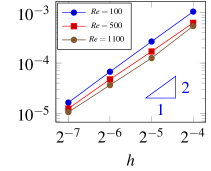
(b) $\left\|u_{y}^{h}-u_{y}\right\|_{L^{2}(\Omega)}$

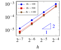
(c) $\left\|p^{h}-p\right\|_{L^{2}(\Omega)}$

Figure 2: Error convergence with linear basis, $\alpha=1$

(a) $\left\|u_{x}^{h}-u_{x}\right\|_{L^{2}(\Omega)}$

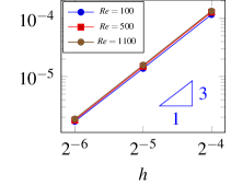
(b) $\left\|u_{y}^{h}-u_{y}\right\|_{L^{2}(\Omega)}$

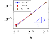
(c) $\left\|p^{h}-p\right\|_{L^{2}(\Omega)}$

Figure 3: Error convergence with quadratic basis, $\alpha=2$

To test the accuracy of the method outlined above, we use the method of manufactured solutions in a spatially two-dimensional problem. We consider a spatiotemporal domain $U=\Omega\times I_{T}$ where the spatial domain $\Omega=[0,1]^{2}\subset\mathbb{R}^{2}$ and the time horizon $I_{T}=[0,1]$. We take the exact solution $(u_{x},u_{y},p)$ to be

$$u_{x} =\sin(\pi x)\cos(\pi y)\sin(t)$$ (71)

$$u_{y} =-\cos(\pi x)\sin(\pi y)\sin(t)$$ (72)

$$p =\sin(\pi x)\sin(\pi y)\cos(t)$$ (73)

such that the velocity vector ${\mathbold{u}}=(u_{x},u_{y})$ satisfies zero divergence, i.e., ${\mathbold{{\nabla}}}\cdot{\mathbold{u}}=0$. We obtain the right hand side forcing ${\mathbold{f}}$ by substituting these exact solutions $(u_{x},u_{y},p)$ in (1). With the obtained forcing ${\mathbold{f}}$, we now solve (32) using both linear ($Q_{1}$) and quadratic ($Q_{2}$) finite elements. The resulting errors in the $L^{2}(U)$-norm are presented for three different Reynolds numbers in Figure 2 for linear elements and in Figure 3 for quadratic elements. On these $\log-\log$ plots, we notice a slope of 2 for linear $Q_{1}$ elements and a slope of 3 for $Q_{2}$ elements. We also notice that the rate of convergence in this problem is independent of the Reynolds number. This result can be compared with the convergence estimates provided in Theorem 3.5. It can be seen that the error estimates provided therein under-predict the order of convergence because of the choice of a different norm.

5.2 Lid Driven Cavity Flow

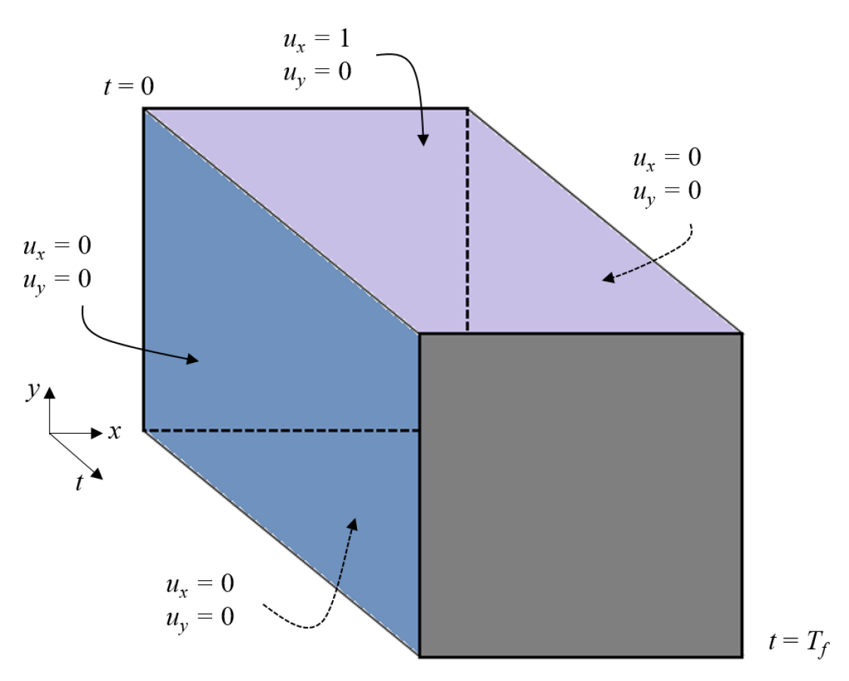
Figure 4: Lid-driven cavity problem definition in space-time

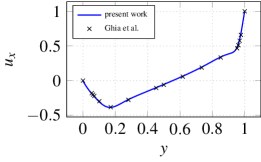
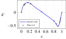
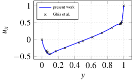
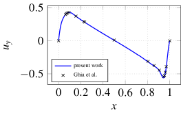
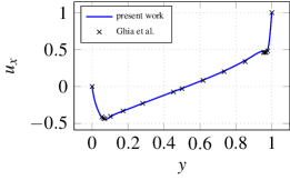
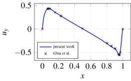
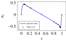
Figure 5: Midline velocity profiles for the lid-driven cavity problem for $Re=1000$ (row-1), $Re=3200$ (row-2), $Re=5000$ (row-3) and $Re=7500$ (row-4). Left column shows $u_{x}$ on a vertical line at $x=0.5$, whereas right column shows $v_{y}$ on a horizontal line at $y=0.5$. Results from Ghia et al. [48] included for comparison.

We test the present method on the well-known “lid-driven cavity” problem. Figure 4 shows a schematic of the “2D version” of this problem, for which, the space-time domain is 3D. Formally, the domain of the problem is $U=D\times I_{T}$, where the spatial domain is $D=[0,1]^{2}\subset\mathbb{R}^{2}$ and the time interval is $I_{T}=[0,T]$. The benchmark results for this problem generally refer to the steady-state solution. Thus, the final time $T$ is chosen such that a steady state is achieved, i.e., $\partial_{t}u_{i}=0,\text{ }i=1,2$ for some $t=t_{s}$; with $T$ being strictly larger than $t_{s}$. The “steady-state” time value ($t_{s}$) increases with increase in the Reynolds number, thus $T$ also grows with $Re$. In the present work, the time-horizon values chosen for the space-time simulations of this problem are $T=180,180,360,720$ for $Re=1000,3200,5000,7500$ respectively.

Figure 5 shows the results obtained for different Reynolds numbers, $Re=$1000, 3200, 5000, 7500, 10000. The left column plots the horizontal velocity $u_{x}$ on a vertical line at $x=0.5$ and $t=T$. In other words, the left column shows the plot of $u_{x}(x=0.5,y,t=T)$ vs. $y$. And similarly, on both figures, the right column plots $u_{y}(x,y=0.5,t=T)$ vs. $x$. The results in Figure 5 compare different solutions with a reference solution. The space-time solution was obtained by taking a large space-time domain of size $[0,1]^{2}\times[0,T]$. The plots in Figure 5 are obtained by taking a slice of the solution on the $t=T$ surface.

5.3 Flow past a circular cylinder

5.3.1 Problem definition

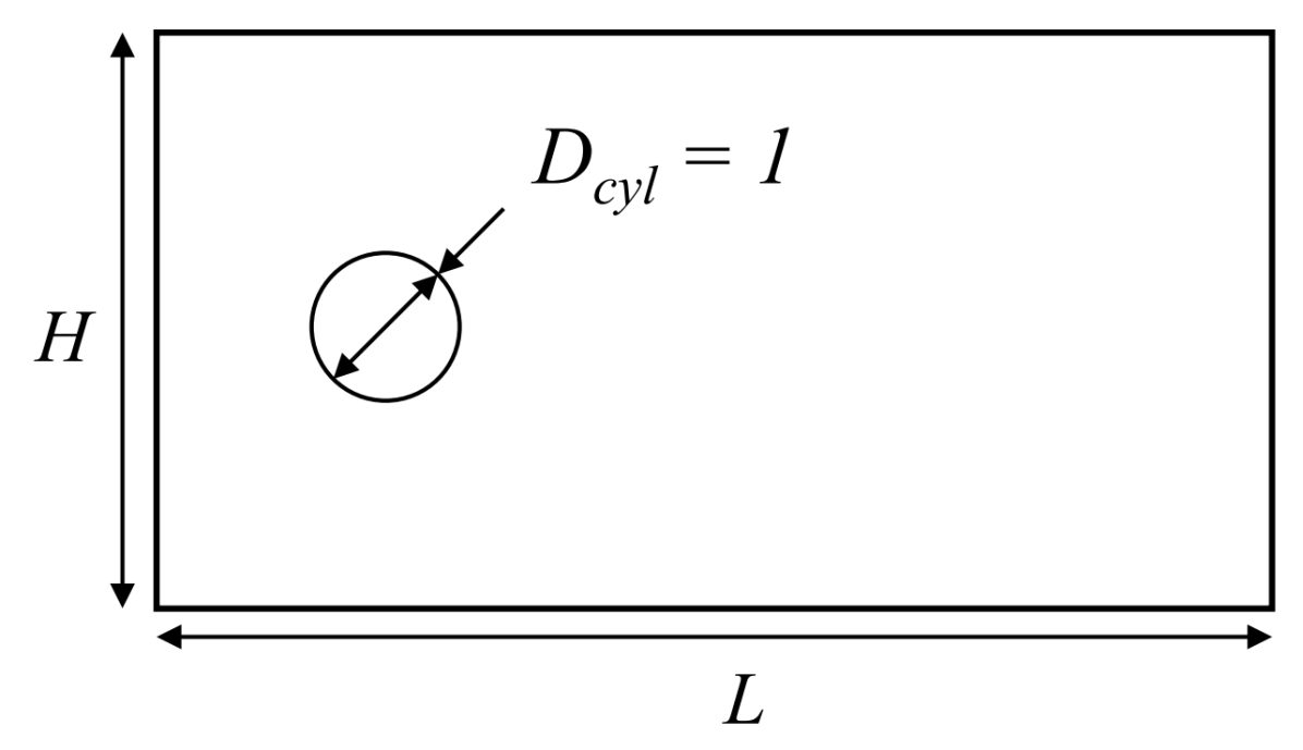
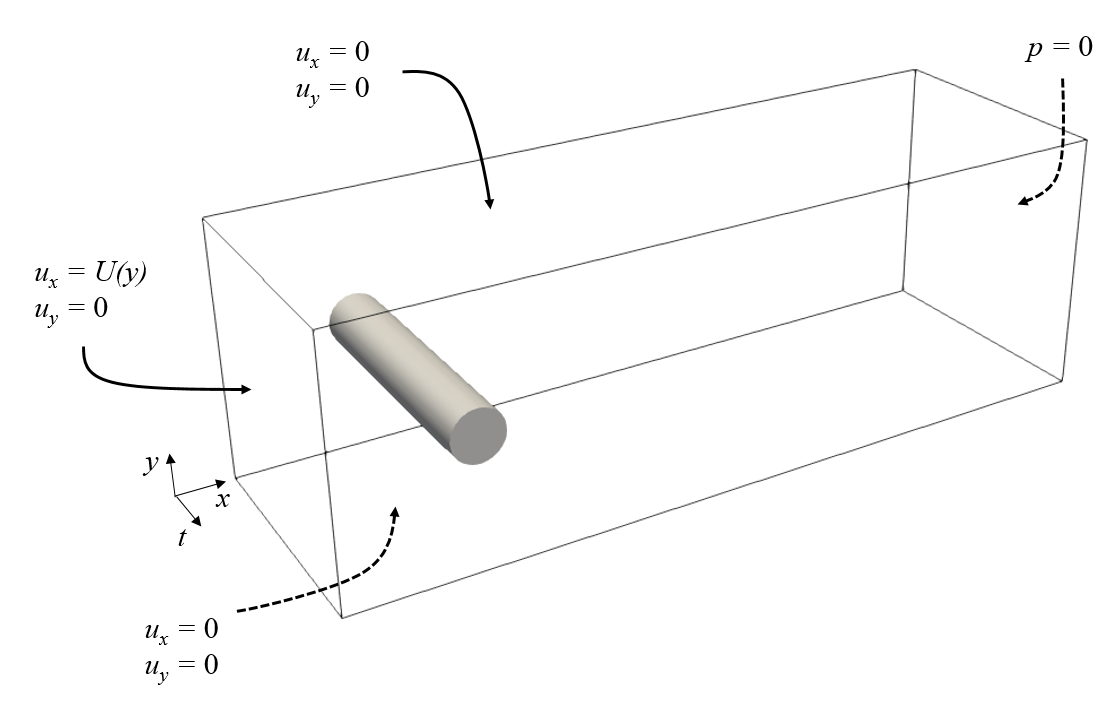
Figure 6: Schematic diagram of the flow past a circular cylinder problem: (left) spatial domain, (right) spatiotemporal domain.

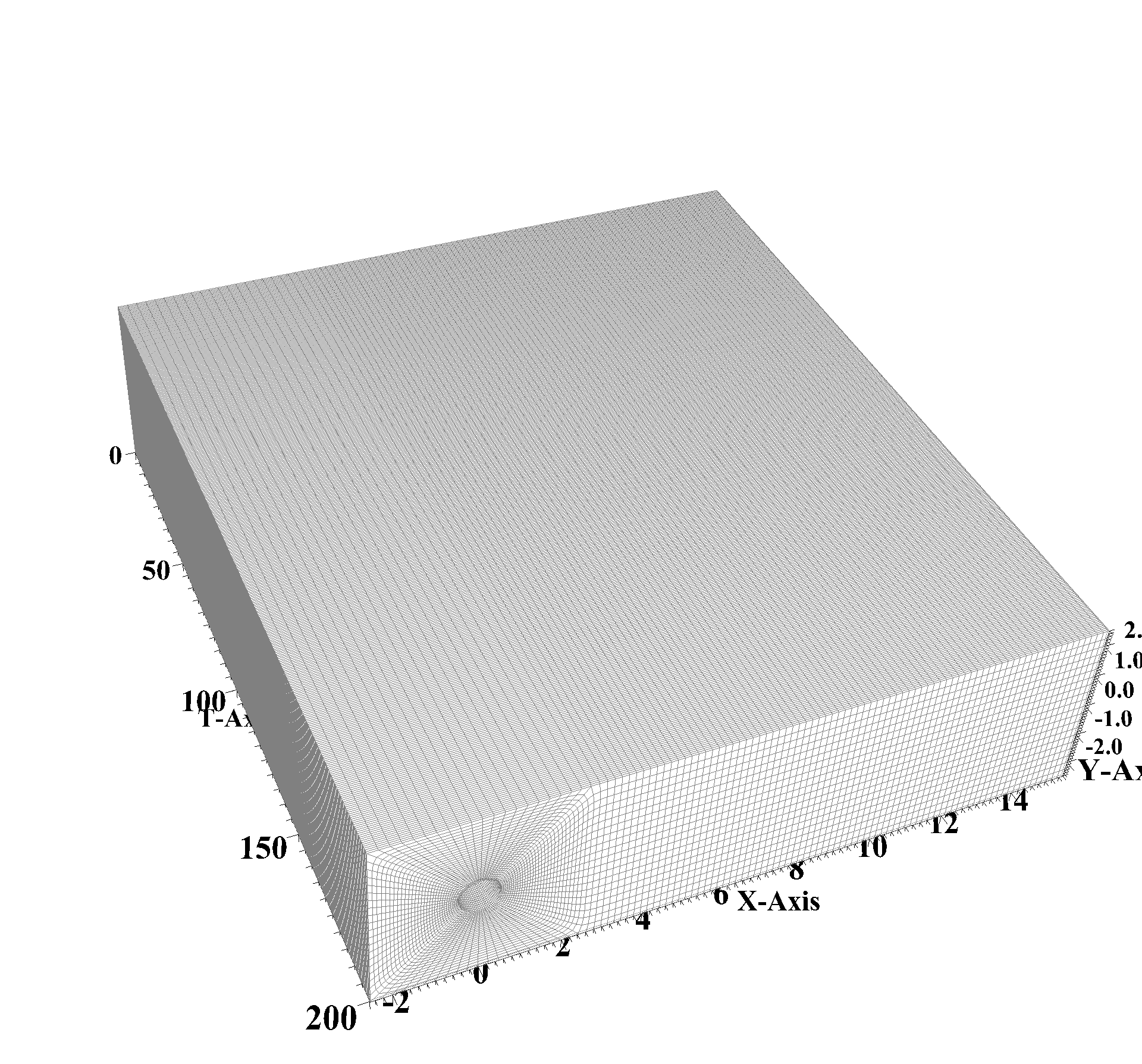
Figure 7: Space-time mesh with hexahedral elements

Next, we test our method on the problem of two-dimensional flow past a circular cylinder. The schematic of the problem is shown in Figure 6. The spatial domain is $D=((I_{x}\times I_{y})\backslash C)$, where $I_{x}=[0,L],\ I_{y}=[0,H]$ and $C$ denotes a circle of diameter $D_{cyl}$ with center at $(x_{c},y_{c})$. The space-time domain $U=D\times I_{t}$. The boundary conditions are specified as:

$$\text{At }x=0:\enspace u_{x}(y,t)=U(y),\quad u_{y}(y,t)=0$$ (74a)

$$\text{At }x=L:\enspace u_{x}(y,t)=u_{y}(y,t)=0$$ (74b)

$$\text{At }y=0:\enspace u_{x}(y,t)=u_{y}(y,t)=0$$ (74c)

$$\text{At }y=H:\enspace u_{x}(y,t)=u_{y}(y,t)=0$$ (74d)

where the inlet flow profile $U(y)$ is given by

$$U(y)=U_{c}\left[1-\left(\frac{1-2y}{H}\right)^{2}\right]$$ (75)

with $U_{c}=1$ being the velocity at $y=\frac{1}{2}$. $U(y)$ has a parabolic profile with $U(0)=U(H)=0$ and $U(\frac{1}{2})=U_{c}=1$. The diameter of the circular cylinder is $D_{cyl}=1$. The Reynolds number for this problem is defined as $Re=\frac{U_{m}D_{cyl}}{\nu}=\frac{1}{\nu}$. For this problem, there exists a critical Reynolds number $Re_{cr}\approx 50$ below which the flow is laminar and reaches a steady state after a certain time $T$ [49]. But for higher Reynolds numbers, the wake becomes unstable with periodic oscillations. In particular, for $90<Re<400$, a clear periodic solution is obtained which create a vortex street in the wake. Below we investigate both these behaviors using the space-time method developed above.

5.3.2 Results for Re=20

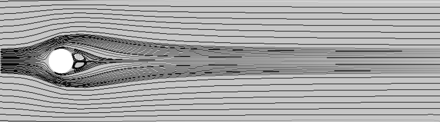
Figure 8: Streamlines for FPC with Re=20

$Re=20$ is well below the critical Reynolds number ($Re_{cr}\sim 50$), thus a steady state exists. As Figure 8 shows, this steady state is achieved with the space-time method. Values of velocity in x and y directions can be observed in Figure 9 and Figure 10. The calculated drag coefficient is $C_{d}=2.75$.

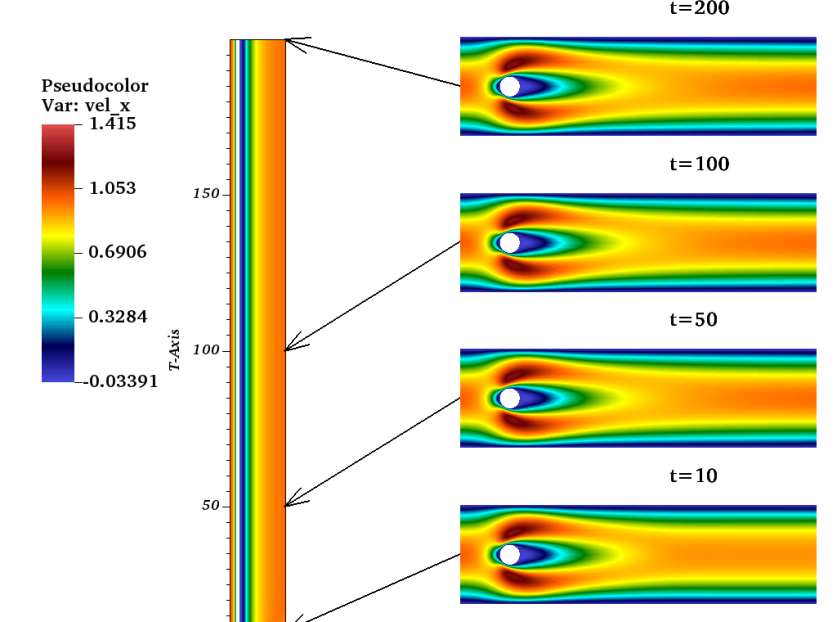
Figure 9: Velocity in x direction for FPC with Re=20

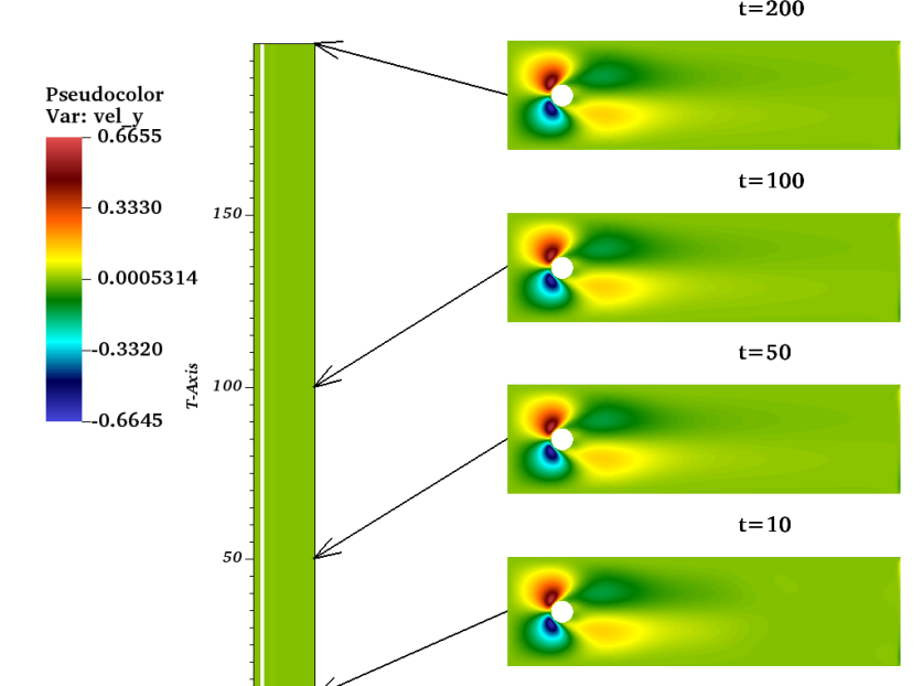
Figure 10: Velocity in y direction for FPC with Re=20

5.3.3 Results for Re=100

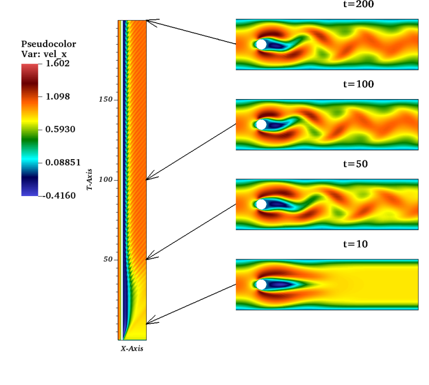
Figure 11: Velocity in x direction for FPC with Re=100

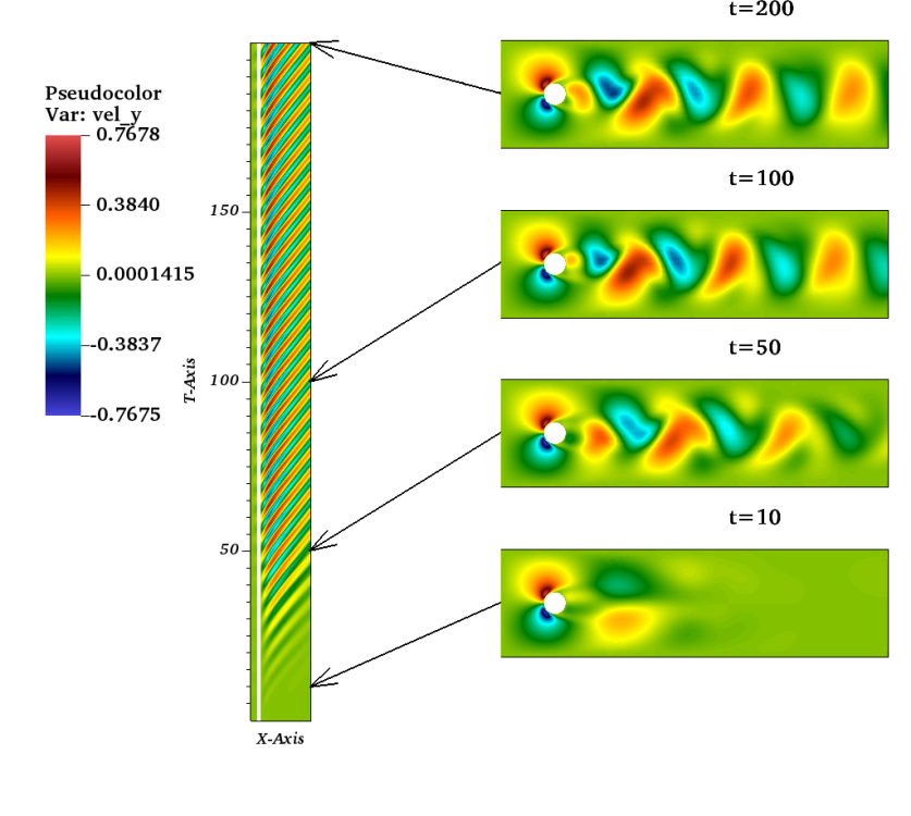
Figure 12: Velocity in y direction for FPC with Re=100

For $75<Re<400$, it is well known that the solution $({\mathbold{u}}_{h},p_{h})$ does not reach a steady state. Rather, a time-periodic behavior emerges after the transient phase. Suppose this problem is solved first with a time-marching algorithm with a time-step of $\Delta t$, starting from an initial time $t=0$. Due to the nature of a time-marching simulation, the solution $({\mathbold{u}}^{t}(x,y),p^{t}(x,y))$ is available only at the discrete times $t=0,\Delta t,2\Delta t,...,n\Delta t,...$ etc. With this setting, the solution $({\mathbold{u}}^{t}(x,y),p^{t}(x,y))$ shows a transient behavior till $t$ reaches a certain value, say, $t_{c}$. After $t_{c}$, the solution continuously becomes periodic with some period $T_{p}$; i.e., $({\mathbold{u}}^{t+T_{p}}(x,y),p^{t+T_{p}}(x,y))=({\mathbold{u}}^{t}(x,y),p^{t}(x,y))$ for $t>t_{c}$.

To recreate this result in a space-time simulation as discussed in Section 2, we need to choose the domain as a tensor product of the same spatial domain $D=(I_{x}\times I_{y})\backslash C$ (see Figure 6, left) and a time interval $I_{T}=[0,T]$ such that $T>t_{c}$ or $[0,t_{c}]\subset I_{T}$. Figure 6 (right) shows a schematic of the spatiotemporal domain.

Figure 7 shows a mesh obtained by discretizing the domain $U$ with hexahedral elements. (32) is solved on this mesh with the boundary conditions given in (74). As discussed in A.1, the simulation needs an initial guess to start. Note that the initial guess refers to a guess for the entire space-time mesh. Coming up with a meaningful guess is non-trivial. In the present case, the initial guess was set to zero for all the nodes in the mesh, except those on the Dirichlet boundaries (this includes the initial-time boundary). Even with this simple initial guess, the Newton-Raphson method is successful in reaching a spatiotemporal solution for this problem. (the method of continuation (Sec. A.2) was not necessary for this simulation.)

Figure 11 shows an $x-t$ slice (at $y=0$) and several $x-y$ slices at multiple $t$-values of the 3D domain. The $x-t$ slice at $y=0$ is seen on the left, with the time-axis extending upward. This slice shows the solution $u_{x}(x,t)|_{y=0}$ evolving in time. Also, we can see from this slice that the solution shows some signs of periodicity around $t=50$ and really falls into a periodic pattern roughly around $t>70$. On the right of Figure 11, we have $u_{x}(x,y)$ plotted as 2D contours at $t=10,50,100,200$. As we expect, the wake starts to develop at $t=10$. At $t=50$, the wake is unstable and shows vortex shedding, but it is not fully periodic yet, as can be confirmed from the $x-t$ slice on the right. At $t=100$ and $t=200$, the shedding has fully developed. Figure 12 shows similar contours for $u_{y}$.

The drag and lift forces are calculated and plotted with respect to time $t$ in Figure 13. The mean drag and the Strouhal number are listed in Table 5.3.3 for Reynolds numbers $100<Re<400$.

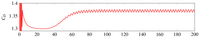
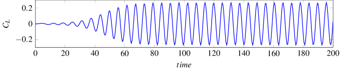
Figure 13: Lift and drag coefficients for Re=100

[ tabular=ccc, table head=$Re$ $C_{d}$ $St$
, late after last line=
] data_files/FPC_study/strouhal_data.txt

Table 1: Mean drag force $C_{d}$ and the Strouhal number ($St$) calculated for various Reynolds number

6 Conclusions

In this paper, we present a method for solving flow problems in space-time using continuous Galerkin finite element method. At the discrete level, such a problem can become unstable when the equation is dominated by the convection term. Also, applying equal-order finite elements for both velocity and pressure can render a non-trivial null space for the pressure solution, thus running into non-uniqueness of pressure. Both these problems can be resolved by formulating the FEM problem using a variational multiscale approach. The application of VMS provides stability against both spatial advection as well as temporal advection (i.e., the time derivative term). It also transforms the saddle point operator into a coercive operator, thus restoring the uniqueness of solutions.

As shown in the numerical results in this paper, the proposed method is able to provide convergence rates as expected. The convergence is both in space and in time. The convergence rate is found to be independent of the Reynolds number. We also tested the method on two benchmark problems, namely, the lid driven cavity problem and the flow past a cylinder problem. Both problems displayed satisfactory results that match previously reported results in the literature.

It can be argued that, everything else being equal, a space-time solution is more expensive than a marching solution for the same problem. But this increased complexity of computation also gives us an opportunity to leverage the scaling capabilities of modern codebases designed for supercomputing facilities. Since the entire time-horizon is included in the mesh, a space-time mesh is extremely well-suited for domain-decomposed analyses. Therefore, even though currently a singular marching simulation is cheaper than a single space-time simulation, it can be shown that with a proper design of scalable codes and proper selection of supercomputing resources, the time-cost of solving PDEs in space-time can be significantly reduced in comparison to time-marching approaches.

Appendix A Solution of the nonlinear system of equations

A.1 Solving nonlinear equations

The FEM problem formulated in (32) is a coupled nonlinear equation. To solve it numerically, we use the Newton-Raphson method [50]. Suppose, the nonlinear system of equations resulting from (32) is written as:

$${\mathbold{b^{g}}}({\mathbold{x^{g}}})={\mathbold{f^{g}}}$$ (76)

where ${\mathbold{b^{g}}}$ and ${\mathbold{f^{g}}}$ are the numerical versions of $B^{h}$ and $F^{h}$; and ${\mathbold{x^{g}}}$ is the vector containing all the unknown discrete degrees of freedoms, i.e.,

$${\mathbold{x^{g}}}=\left(u_{x1},u_{y1},u_{z1},p_{1},u_{x2},u_{y2},u_{z2},p_{2},...,u_{xN},u_{yN},u_{zN},p_{N}\right)$$ (77)

where $N$ is the total number of nodes in the discretization $K^{h}$. Assume that the unknown vector at the $r^{th}$ iteration is denoted as ${\mathbold{x^{g}}}_{r}$. Then following the Newton-Raphson methodology, the $(r+1)^{th}$-step is linearized in the neighborhood of ${\mathbold{x^{g}}}_{r}$ as:

$${\mathbold{J}}({\mathbold{x^{g}}}_{r})\cdot\delta{\mathbold{x^{g}}}_{r}={\mathbold{z^{g}}}$$ (78)

where ${\mathbold{z^{g}}}=\left({\mathbold{f^{g}}}-{\mathbold{b^{g}}}({\mathbold{x^{g}}}_{r})\right)$ is a known vector and ${\mathbold{J}}$ is the Jacobian matrix, whose $(i,j)$ element is the first derivative of the $i$-th element of ${\mathbold{b^{g}}}$ with respect to the $j$-th element of ${\mathbold{x^{g}}}$, i.e., $J_{ij}=\frac{\partial b^{g}_{i}}{\partial x^{g}_{j}}$. (78) is now solved for $\delta{\mathbold{x^{g}_{r}}}$ and then ${\mathbold{x^{g}}}_{r+1}$ is obtained from:

$${\mathbold{x^{g}}}_{r+1}={\mathbold{x^{g}}}_{r}+\delta{\mathbold{x^{g}}}_{r},\quad r=0,1,2,...$$ (79)

${\mathbold{x^{g}}}_{0}$ is the initial guess provided at the start of the Newton-Raphson iterations. The iteration is stopped when the norm of the increment vector ${\mathbold{x}}^{{\mathbold{g}}}_{r}$ is less than some previously set tolerance value $\gamma>0$, i.e., when $\left\|\delta{\mathbold{x}}^{{\mathbold{g}}}_{r}\right\|\leq\gamma$, where usually $\gamma$ is a small real number.

The key step in the linear algebra problem is now (78) which requires the solution of a large linear algebraic system. We use PETSc [51] for solving this linear system. Once the global Jacobian matrix ${\mathbold{J}}$ and the global right hand side ${\mathbold{z^{g}}}$ are assembled, PETSc functions are called to solve (78) for $\delta{\mathbold{x^{g}}}_{r}$. Once again, since the dimensionality of the problem is high, so is the size of ${\mathbold{J}}$. Thus, direct/non-iterative solvers such as LU-decomposition (with complexity $O(n^{3})$, $n=$ matrix size) become very inefficient. Iterative methods, on the other hand, take about $\sim O(mn)$ time [52] (where $m$ is the number of iterations, $m\ll n$) for sparse matrices, and are therefore preferred.

A.2 Method of Continuation

A space-time formulation, as described in this paper, is by definition non-evolutionary. It is seen in (32) which is formulated over a Hilbert space whose underlying domain is spatio-temporal; and consequently the algebraic problem in (76) or (78) contain unknowns that span the full spatio-temporal domain $\Omega$. When solving such equations using the Newton-Raphson scheme (78), an initial guess for ${\mathbold{x}}^{{\mathbold{g}}}_{r}$ is required. One common characteristic of the Newton-Raphson method is that the convergence of system (78) depends on the quality of the initial guess ${\mathbold{x}}^{\mathbold{g}}_{r}$. Suppose the exact solution of the system (76) is ${\mathbold{x}}^{\mathbold{g}}_{*}$. Then, if $\|{\mathbold{x}}^{\mathbold{g}}_{0}-{\mathbold{x}}^{\mathbold{g}}_{*}\|$ is large, then the scheme (78) and (79) might fail to converge to ${\mathbold{x}}^{\mathbold{g}}_{*}$. In these cases, we cannot simply rely solely on the increment $\delta{\mathbold{x}}^{{\mathbold{g}}}_{r}$ provided by the Newton-Raphson scheme (78).

Thus, to overcome this issue, we use a variant of the method of continuation, known as the pseudo-transient continuation (PTC) [53, 54]. We do this by embedding the fully coupled space-time system of equations (76) in an auxiliary evolution space $\tau$ as follows:

$$\frac{\partial{\mathbold{x^{g}}}}{\partial\tau}+{\mathbold{b^{g}}}({\mathbold{x^{g}}})={\mathbold{f^{g}}}.$$ (80)

If we compare (80) with (76), we can infer the role of the variable $\tau$. In the ideal case, we want (80) and (76) to yield the same solution for ${\mathbold{x^{g}}}$, thereby making $\frac{\partial{\mathbold{x^{g}}}}{\partial\tau}=0$. This gives us an opportunity to design an iteration scheme similar to a time-marching algorithm that “evolves” the space-time solution ${\mathbold{x^{g}}}$ with respect to $\tau$. Assume a discretization of the auxiliary variable $\tau$ given by $\tau^{h}=(\tau^{0},\tau^{1},...)$, where the elements in $\tau^{h}$ are not necessarily equidistant. With this, we can approximate (80) as

$$\frac{{\mathbold{x}}^{{\mathbold{g}}^{k+1}}-{\mathbold{x}}^{{\mathbold{g}}^{k}}}{\Delta\tau^{k+1}}+{\mathbold{b^{g}}}({\mathbold{x}}^{{\mathbold{g}}^{k+1}}) ={\mathbold{f^{g}}}$$ (81)

$$\implies\quad\quad\frac{{\mathbold{x}}^{{\mathbold{g}}^{k+1}}}{\Delta\tau^{k+1}}+{\mathbold{b^{g}}}({\mathbold{x}}^{{\mathbold{g}}^{k+1}}) =\frac{{\mathbold{x}}^{{\mathbold{g}}^{k}}}{\Delta\tau^{k+1}}+{\mathbold{f^{g}}},\quad k=0,1,2,...,$$ (82)

where $\Delta\tau^{k+1}=\tau^{k+1}-\tau^{k}$. With a sufficiently small choice of $\Delta\tau^{k+1}$, (82) is a contraction for ${\mathbold{x^{g}}}$, i.e., there exists a $K^{\infty}\in\mathbb{N}$ such that $\|{\mathbold{x}}^{{\mathbold{g}}^{k}}-{\mathbold{x}}^{{\mathbold{g}}}_{*}\|\leq\epsilon$ for all $k\geq K^{\infty}$. At $k=0$, we do not have a solution, rather, we just have an initial guess denoted by ${\mathbold{x}}^{{\mathbold{g}}^{0}}$. But as we solve (82) successively, each ${\mathbold{x}}^{{\mathbold{g}}^{k}}$ gets closer and closer to the true solution ${\mathbold{x}}^{{\mathbold{g}}}_{*}$.

(82) is still nonlinear in ${\mathbold{x^{g}}}$. Thus applying Newton-Raphson linearization to (82), we have:

$$\left[\frac{{\mathbold{M}}}{\Delta\tau^{k+1}}+{\mathbold{J}}({\mathbold{x}}^{{\mathbold{g}}^{k+1}}_{r})\right]\cdot\delta{\mathbold{x}}^{{\mathbold{g}}^{k+1}}_{r} ={\mathbold{z}}^{{\mathbold{g}}^{k+1}},$$ (83)

$${\mathbold{x}}^{{\mathbold{g}}^{k+1}}_{r+1} ={\mathbold{x}}^{{\mathbold{g}}^{k+1}}_{r}+\delta{\mathbold{x}}^{{\mathbold{g}}^{k+1}}_{r},\quad r=0,1,2,...$$ (84)

where ${\mathbold{z}}^{{\mathbold{g}}^{k+1}}=\left({\mathbold{x}}^{{\mathbold{g}}^{k}}/\Delta\tau^{k+1}+{\mathbold{f^{g}}}-{\mathbold{b^{g}}}({\mathbold{x}}^{{\mathbold{g}}^{k}}_{r})\right)$.

Once again, iteration (84) is stopped when $\left\|\delta{\mathbold{x}}^{{\mathbold{g}}^{k+1}}_{r}\right\|<\gamma_{1}$, and the backward Euler iterations (82) are stopped when $\left\|{\mathbold{x}}^{{\mathbold{g}}^{k+1}}-{\mathbold{x}}^{{\mathbold{g}}^{k}}\right\|<\gamma_{2}$, where $\gamma_{1}>0$ and $\gamma_{2}>0$ are preset tolerances of a small magnitude.

Appendix B Numerical linear solver options

B.1 Lid-driven Cavity

All simulations in this paper were done using the linear algebra solvers provided by PETSc. Below are the command line options for the PETSc linear solvers. $T$ refers to the physical time horizon of the space-time domain.

The common options used in all cases:

⬇

-ksp_rtol 1e-6 #default

-snes_rtol 1e-8

-snes_atol 1e-8

Case-by-case options are as follows:

• $Re=1000$, $T=180$
  (a) mesh: $32^{3}$ ⬇ -ksp_type ibcgs -pc_type asm -snes_ksp_ew (a) mesh : $128^{3}$ ⬇ -ksp_type bcgsl -pc_type bjacobi #default

• $Re=3200$, $T=180$
  (a) mesh: $32^{3}$ ⬇ -ksp_type ibcgs -pc_type asm -snes_ksp_ew (a) mesh : $128^{3}$ ⬇ -ksp_type bcgsl -pc_type bjacobi #default

• $Re=5000$, $T=360$
  (a) mesh: $32^{3}$ ⬇ -ksp_type ibcgs -pc_type asm (a) mesh : $128^{3}$ ⬇ -ksp_type ibcgs -pc_type asm -snes_ksp_ew

• $Re=7500$, $T=720$
  (a) mesh: $32^{3}$ ⬇ -ksp_type bcgsl -pc_type bjacobi #default (a) mesh : $128^{3}$ ⬇ -ksp_type ibcgs -pc_type asm -snes_ksp_ew

• $Re=10,000$, $T=10^{3}$
  (a) mesh: $32^{3}$ ⬇ -ksp_type bcgsl -pc_type bjacobi #default (a) mesh : $128^{3}$ ⬇ -- (not run)

References

- [1] Jürg Nievergelt. Parallel methods for integrating ordinary differential equations. Communications of the ACM, 7(12):731–733, 1964.
- [2] Wolfgang Hackbusch. Parabolic multi-grid methods. In Proc. Of the Sixth Int’L. Symposium on Computing Methods in Applied Sciences and Engineering, VI, pages 189–197, Amsterdam, The Netherlands, The Netherlands, 1985. North-Holland Publishing Co.
- [3] Philippe Chartier and Bernard Philippe. A parallel shooting technique for solving dissipative ode’s. Computing, 51(3):209–236, 1993.
- [4] Graham Horton and Stefan Vandewalle. A space-time multigrid method for parabolic partial differential equations. SIAM Journal on Scientific Computing, 16(4):848–864, 1995.
- [5] Martin Jakob Gander. Overlapping schwarz for linear and nonlinear parabolic problems. In 9th International Conference on Domain Decomposition Methods, pages 97–104, 1996.
- [6] Martin Jakob Gander, Laurence Halpern, and Frédéric Nataf. Optimal convergence for overlapping and non-overlapping schwarz waveform relaxation. In 11th international conference on domain decomposition methods, pages 27–36, 1999.
- [7] J.-L. Lions, Yvon Maday, and Gabriel Turinici. A ”parareal” in time discretization of PDE’s. Comptes Rendus de l’Académie des Sciences - Series I - Mathematics, 332:661–668, 2001.
- [8] Martin J Gander. 50 years of time parallel time integration. In Multiple Shooting and Time Domain Decomposition Methods, pages 69–113. Springer, 2015.
- [9] Prasenjit Saha, Joachim Stadel, and Scott Tremaine. A parallel integration method for solar system dynamics. arXiv preprint astro-ph/9605016, 1996.
- [10] Ch Lubich and A Ostermann. Multi-grid dynamic iteration for parabolic equations. BIT Numerical Mathematics, 27(2):216–234, 1987.
- [11] Robert Dyja, Baskar Ganapathysubramanian, and Kristoffer G van der Zee. Parallel-in-space-time, adaptive finite element framework for nonlinear parabolic equations. SIAM Journal on Scientific Computing, 40(3):C283–C304, 2018.
- [12] Thomas JR Hughes and Gregory M Hulbert. Space-time finite element methods for elastodynamics: formulations and error estimates. Computer methods in applied mechanics and engineering, 66(3):339–363, 1988.
- [13] Gregory M Hulbert and Thomas JR Hughes. Space-time finite element methods for second-order hyperbolic equations. Computer methods in applied mechanics and engineering, 84(3):327–348, 1990.
- [14] JP Pontaza and JN Reddy. Space–time coupled spectral/hp least-squares finite element formulation for the incompressible navier–stokes equations. Journal of Computational Physics, 197(2):418–459, 2004.
- [15] Tayfun E Tezduyar, Sunil Sathe, Ryan Keedy, and Keith Stein. Space–time finite element techniques for computation of fluid–structure interactions. Computer methods in applied mechanics and engineering, 195(17-18):2002–2027, 2006.
- [16] Tayfun E Tezduyar, Sunil Sathe, Matthew Schwaab, and Brian S Conklin. Arterial fluid mechanics modeling with the stabilized space–time fluid–structure interaction technique. International Journal for Numerical Methods in Fluids, 57(5):601–629, 2008.
- [17] Martin J Gander and Martin Neumuller. Analysis of a new space-time parallel multigrid algorithm for parabolic problems. SIAM Journal on Scientific Computing, 38(4):A2173–A2208, 2016.
- [18] Marek Behr. Simplex space–time meshes in finite element simulations. International journal for numerical methods in fluids, 57(9):1421–1434, 2008.
- [19] Olaf Steinbach. Space-time finite element methods for parabolic problems. Computational methods in applied mathematics, 15(4):551–566, 2015.
- [20] Ulrich Langer, Stephen E Moore, and Martin Neumüller. Space–time isogeometric analysis of parabolic evolution problems. Computer methods in applied mechanics and engineering, 306:342–363, 2016.
- [21] Thomas Führer and Michael Karkulik. Space–time least-squares finite elements for parabolic equations. Computers & Mathematics with Applications, 92:27–36, 2021.
- [22] Masado Ishii, Milinda Fernando, Kumar Saurabh, Biswajit Khara, Baskar Ganapathysubramanian, and Hari Sundar. Solving pdes in space-time: 4d tree-based adaptivity, mesh-free and matrix-free approaches. In Proceedings of the International Conference for High Performance Computing, Networking, Storage and Analysis, pages 1–61, 2019.
- [23] Roman Andreev. Stability of space-time Petrov-Galerkin discretizations for parabolic evolution equations. PhD thesis, ETH Zurich, 2012.
- [24] Alexander N Brooks and Thomas JR Hughes. Streamline upwind/petrov-galerkin formulations for convection dominated flows with particular emphasis on the incompressible navier-stokes equations. Computer methods in applied mechanics and engineering, 32(1-3):199–259, 1982.
- [25] Thomas JR Hughes, Leopoldo P Franca, and Gregory M Hulbert. A new finite element formulation for computational fluid dynamics: Viii. the galerkin/least-squares method for advective-diffusive equations. Computer methods in applied mechanics and engineering, 73(2):173–189, 1989.
- [26] Jim Douglas and Jun Ping Wang. An absolutely stabilized finite element method for the stokes problem. Mathematics of computation, 52(186):495–508, 1989.
- [27] Thomas JR Hughes. Multiscale phenomena: Green’s functions, the dirichlet-to-neumann formulation, subgrid scale models, bubbles and the origins of stabilized methods. Computer methods in applied mechanics and engineering, 127(1-4):387–401, 1995.
- [28] Thomas JR Hughes, Leopoldo P Franca, and Marc Balestra. A new finite element formulation for computational fluid dynamics: V. circumventing the babuška-brezzi condition: A stable petrov-galerkin formulation of the stokes problem accommodating equal-order interpolations. Computer Methods in Applied Mechanics and Engineering, 59(1):85–99, 1986.
- [29] Y Bazilevs, VM Calo, JA Cottrell, TJR Hughes, A Reali, and G Scovazzi. Variational multiscale residual-based turbulence modeling for large eddy simulation of incompressible flows. Computer methods in applied mechanics and engineering, 197(1-4):173–201, 2007.
- [30] Roger Temam. Une méthode d’approximation de la solution des équations de navier-stokes. Bulletin de la Société Mathématique de France, 96:115–152, 1968.
- [31] Jie Shen. On error estimates of the projection methods for the navier-stokes equations: second-order schemes. Mathematics of computation, 65(215):1039–1065, 1996.
- [32] Jie Shen. Pseudo-compressibility methods for the unsteady incompressible navier-stokes equations.
- [33] Ramon Codina. A stabilized finite element method for generalized stationary incompressible flows. Computer methods in applied mechanics and engineering, 190(20-21):2681–2706, 2001.
- [34] Ivo Babuška. The finite element method with lagrangian multipliers. Numerische Mathematik, 20(3):179–192, 1973.
- [35] Franco Brezzi. On the existence, uniqueness and approximation of saddle-point problems arising from lagrangian multipliers. Publications mathématiques et informatique de Rennes, (S4):1–26, 1974.
- [36] Volker John. Finite element methods for incompressible flow problems. Springer, 2016.
- [37] Ramon Codina. Comparison of some finite element methods for solving the diffusion-convection-reaction equation. Computer methods in applied mechanics and engineering, 156(1-4):185–210, 1998.
- [38] Tayfun E Tezduyar, Sanjay Mittal, SE Ray, and R Shih. Incompressible flow computations with stabilized bilinear and linear equal-order-interpolation velocity-pressure elements. Computer Methods in Applied Mechanics and Engineering, 95(2):221–242, 1992.
- [39] Thomas JR Hughes, Michel Mallet, and Mizukami Akira. A new finite element formulation for computational fluid dynamics: Ii. beyond supg. Computer methods in applied mechanics and engineering, 54(3):341–355, 1986.
- [40] Farzin Shakib, Thomas JR Hughes, and Zdeněk Johan. A new finite element formulation for computational fluid dynamics: X. the compressible euler and navier-stokes equations. Computer Methods in Applied Mechanics and Engineering, 89(1-3):141–219, 1991.
- [41] Claes Johnson. Numerical solution of partial differential equations by the finite element method. Courier Corporation, 2012.
- [42] Tian Xiao Zhou and Min Fu Feng. A least squares petrov-galerkin finite element method for the stationary navier-stokes equations. mathematics of computation, 60(202):531–543, 1993.
- [43] Philippe G Ciarlet. The finite element method for elliptic problems. SIAM, 2002.
- [44] Lawrence C Evans. Partial differential equations, volume 19. American Mathematical Society, 2022.
- [45] Susanne Brenner and Ridgway Scott. The mathematical theory of finite element methods, volume 15. Springer Science & Business Media, 2007.
- [46] JT (John Tinsley) Oden and Junuthula Narasimha Reddy. An introduction to the mathematical theory of finite elements. John Wiley & Sons, Limited, 1976.
- [47] George Karypis, Kirk Schloegel, and Vipin Kumar. Parmetis. Parallel graph partitioning and sparse matrix ordering library. Version, 2, 2003.
- [48] UKNG Ghia, Kirti N Ghia, and CT Shin. High-re solutions for incompressible flow using the navier-stokes equations and a multigrid method. Journal of computational physics, 48(3):387–411, 1982.
- [49] Momchilo M Zdravkovich. Flow around circular cylinders. Fundamentals, 1:566–571, 1997.
- [50] Randall J LeVeque. Finite difference methods for ordinary and partial differential equations: steady-state and time-dependent problems. SIAM, 2007.
- [51] Satish Balay, Kris Buschelman, William D Gropp, Dinesh Kaushik, Matthew G Knepley, L Curfman McInnes, Barry F Smith, and Hong Zhang. Petsc. See http://www. mcs. anl. gov/petsc, 2001.
- [52] Lloyd N Trefethen and David Bau III. Numerical linear algebra, volume 50. Siam, 1997.
- [53] Todd S Coffey, Carl Tim Kelley, and David E Keyes. Pseudotransient continuation and differential-algebraic equations. SIAM Journal on Scientific Computing, 25(2):553–569, 2003.
- [54] Carl Timothy Kelley and David E Keyes. Convergence analysis of pseudo-transient continuation. SIAM Journal on Numerical Analysis, 35(2):508–523, 1998.