Multilinear Mixture of Experts:
Scalable Expert Specialization through Factorization

Abstract

The Mixture of Experts (MoE) paradigm provides a powerful way to decompose inscrutable dense layers into smaller, modular computations often more amenable to human interpretation, debugging, and editability. A major problem however lies in the computational cost of scaling the number of experts to achieve sufficiently fine-grained specialization. In this paper, we propose the Multilinear Mixutre of Experts (MMoE) layer to address this, focusing on vision models. MMoE layers perform an implicit computation on prohibitively large weight tensors entirely in factorized form. Consequently, MMoEs both (1) avoid the issues incurred through the discrete expert routing in the popular ‘sparse’ MoE models, yet (2) do not incur the restrictively high inference-time costs of ‘soft’ MoE alternatives. We present both qualitative and quantitative evidence (through visualization and counterfactual interventions respectively) that scaling MMoE layers when fine-tuning foundation models for vision tasks leads to more specialized experts at the class-level whilst remaining competitive with the performance of parameter-matched linear layer counterparts. Finally, we show that learned expert specialism further facilitates manual correction of demographic bias in CelebA attribute classification. Our MMoE model code is available at https://github.com/james-oldfield/MMoE.

1 Introduction

The Mixture of Experts (MoE) architecture (Jacobs et al., 1991b) has reemerged as a powerful class of conditional computation, underpinning a lot of recent breakthroughs in machine learning. In its essence, MoEs apply different subsets of layers (referred to as ‘experts’) for each input, in contrast to the traditional approach of applying the same single layer to all inputs. This provides a form of input-conditional computation (Ha et al., 2017; Vaswani et al., 2017; Han et al., 2021; Chen et al., 2020) that is expressive yet efficient. One popular modern incarnation is the sparsely gated MoE (Shazeer et al., 2017), which allows for significant model capacity increases without commensurate increases to computational costs (Lepikhin et al., 2021; Fedus et al., 2022; Gale et al., 2023). Consequently, MoEs have been the key mechanism in scaling up large language (Jiang et al., 2024), vision (Riquelme et al., 2021), and multi-modal models (Mustafa et al., 2022), achieving remarkable performance across the board.

However, through their substantial performance gains, an important emergent property of MoEs is frequently underutilized: the innate tendency of experts to specialize in distinct subtasks. In other words, MoEs often naturally learn a form of weight disentanglement (Ortiz-Jimenez et al., 2023). Indeed, the foundational work of Jacobs et al. (1991a) on MoEs describes this property, highlighting how implementing a particular function with modular building blocks (experts) often leads to subcomputations that are easier to understand individually than their dense layer counterparts. Independent of model performance, a successful decomposition of the layer’s functionality into human-comprehensible subtasks offers many significant benefits. Firstly, the mechanisms through which a network produces an output are more interpretable: the output is a sum of modular components, each contributing individual functionality. Yet, the value of interpretable computation extends beyond just transparency (Lipton, 2018) and explainability (Ribeiro et al., 2016). An important corollary of successful task decomposition amongst experts is that layers are easier to debug and edit. Biased or unsafe behaviors can be better localized to specific experts’ subcomputation, facilitating manual correction or surgery in a way that minimally affects the other functionality of the network. Addressing such behaviors is particularly crucial in the context of foundation models; being often fine-tuned as black boxes pre-trained on unknown, potentially unbalanced data distributions. Furthermore, there is evidence that traditional fairness techniques are less effective in large-scale models (Mao et al., 2023; Cherepanova et al., 2021). However, to achieve fine-grained expert specialism at the class level (or more granular still), one needs the ability to significantly scale up the number of experts. Alas, the dominating sparse MoE (Shazeer et al., 2017) has several difficulties achieving this due to the discrete expert selection step–often leading to training instability and difficulties in scaling the total expert count, amongst other issues described in Mohammed et al. (2022); Puigcerver et al. (2024).

In this paper, we propose the Multilinear Mixture of Experts (MMoE) layer to exploit the inductive bias and subtask specialism that emerges from MoEs at a large scale. MMoEs are designed to scale gracefully to tens of thousands of experts–without the need for any non-differentiable operations–through implicit computations on a factorized form of the experts’ weights. Furthermore, MMoEs readily generalize to multiple hierarchies, intuitively implementing “and” operators in expert selection at each level–further providing a mechanism to increase both expert specificity, and total expert count. Crucially, we show evidence that scaling up the number of MMoE experts leads to increased expert specialism when fine-tuning foundation models for vision tasks. Our evidence is provided in three forms: (1) firstly, through the usual qualitative evaluation of inspecting images by their expert coefficients. Secondly (2), we further explore the causal role of each expert through counterfactual interventions (Elazar et al., 2021). Finally, (3) we show how MMoE expert specialism facilitates the practical task of model editing–how subcomputation in specific combinations of experts biased towards demographic subpopulations can be manually corrected through straightforward guided edits. Our multilinear generalization reveals intriguing connections between various classes of models: (1) MMoEs recover linear MoEs as a special case, and (2) MoE tensorization allows us to reformulate (linear) MoEs as a specific form of bilinear layer. Interestingly, both MoEs and bilinear layers individually have been hypothesized to be useful for mechanistic interpretability in Elhage et al. (2022) and Sharkey (2023) respectively, for different reasons. The unification of the two through MMoEs underscores the potential value of the proposed layer for wider interpretability endeavors.

Our contributions and core claims can be summarized as follows:

• We introduce MMoE layers–a mechanism for computing vast numbers of subcomputations and efficiently fusing them conditionally on the input (with nested levels of hierarchy).

• We show both qualitatively (through visualization) and quantitatively (through counterfactual intervention) that increasing the number of MMoE experts increases task modularity–learning to specialize in processing just specific input classes when fine-tuning large foundation models for vision tasks.

• We further demonstrate how the MMoE architecture allows manual editing of combinations of experts to address the task of mitigating demographic bias in CelebA attribute classification, improving fairness metrics over existing baselines without any fine-tuning.

• We establish experimentally that MMoE layers are competitive with parameter-matched linear layer counterparts when used to fine-tune CLIP and DINO backbones for downstream image classification.

2 Related Work

Mixture of Experts

Recent years have seen a resurgence of interest in the Mixture of Experts (MoE) architecture for input-conditional computation (Shazeer et al., 2017; Jacobs et al., 1991a; Bengio et al., 2015; Jiang et al., 2024). One primary motivation for MoEs is their increased model capacity through large parameter count (Shazeer et al., 2017; Fedus et al., 2022; Jiang et al., 2024). In contrast to a single dense layer, the outputs of multiple experts performing separate computations are combined (sometimes with multiple levels of hierarchy (Jordan & Jacobs, 1993; Eigen et al., 2013)). A simple approach to fusing the outputs is by taking either a convex (Eigen et al., 2013) or linear (Yang et al., 2019) combination of the output of each expert. The seminal work of Shazeer et al. (2017) however proposes to take a sparse combination of only the top-$K$ most relevant experts, greatly reducing the computational costs of evaluating them all. More recent works employ a similar sparse gating function to apply just a subset of experts (Jiang et al., 2024; Du et al., 2022), scaling to billions (Lepikhin et al., 2021) and trillions of parameters (Fedus et al., 2022). The discrete expert selection choice of sparse MoEs is not without its problems, however–often leading to several issues including training stability and expert under-utilization (Mohammed et al., 2022; Puigcerver et al., 2024).

Particularly relevant to this paper are works focusing on designing MoE models to give rise to more interpretable subcomputation (Gupta et al., 2022; Gururangan et al., 2022; Ismail et al., 2023)–hearkening back to one of the original works of Jacobs et al. (1991a), where experts learned subtasks of discriminating between different lower/uppercase vowels. Indeed a common observation is that MoE experts appear to specialize in processing inputs with similar high-level features. Researchers have observed MoE experts specializing in processing specific syntax (Shazeer et al., 2017) and parts-of-speech (Lewis et al., 2021) for language models, and foreground/background (Wu et al., 2022) and image categories (e.g. ‘wheeled vehicles’) (Yang et al., 2019) in vision. Evidence of shared vision-language specialism is even found in the multi-modal MoEs of Mustafa et al. (2022). However, all of the above works hypothesize expert specialism based on how the input data is routed to experts. No attempts are made to quantify the functional role of the experts in producing the output–either through ablations (Casper, 2023), or causal interventions (Elazar et al., 2021; Meng et al., 2022; Ravfogel et al., 2021). In contrast, our work aims to provide quantitative evidence for expert specialism in two complementary ways: first by asking specific counterfactual questions (Elazar et al., 2021) about the experts’ contribution, and then subsequently by directly editing the hypothesized combination of experts responsible for processing target inputs.

Several works instead target how to make conditional computation more efficient: by sharing expert parameters across layers (Xue et al., 2022), factorizing gating network parameters (Davis & Arel, 2013), or dynamic convolution operations (Li et al., 2021). Relatedly, Gao et al. (2022) jointly parameterize the experts’ weight matrices with a Tensor-Train decomposition (Oseledets, 2011). Such approach still suffers from the Sparse MoE’s instability and expert under-utilization issues however, and stochastic masking of gradients must be performed to lead to balanced experts. Furthermore, whilst Gao et al. (2022) share parameters across expert matrices, efficient implicit computation of thousands of experts simultaneously is not facilitated, in contrast to the MMoE layer.

Factorized layers

in the context of deep neural networks provide several important benefits. Replacing traditional operations with low-rank counterparts allows efficient fine-tuning (Hu et al., 2021) / training (Novikov et al., 2015; Garipov et al., 2016), and modeling of higher-order interactions (Novikov et al., 2017; Georgopoulos et al., 2021; Babiloni et al., 2020; Georgopoulos et al., 2020; Cheng et al., 2024), and convolutions (Kossaifi et al., 2020). In addition to reducing computational costs, tensor factorization has also proven beneficial in the context of multi-task/domain learning (Bulat et al., 2020; Yang & Hospedales, 2017) through the sharing of parameters/low-rank factors across tasks. Furthermore, parameter efficiency through weight factorization often facilitates the design and efficient implementation of novel architectures such as polynomial networks (Chrysos et al., 2020, 2021; Babiloni et al., 2021) or tensor contraction layers (Kossaifi et al., 2017). The recent DFC layer in Babiloni et al. (2023) also performs dynamic computation using the CP decomposition (Hitchcock, 1927) like MMoEs. Despite this technical similarity, the two works have very different goals and model properties due to how the weight matrices are generated. MMoEs take a sparse, convex combination of $N$ explicit experts’ latent factors. This consequently leads to specialized subcomputations in a way that facilitates the interpretability and editability presented in this paper. DFCs can be seen to apply an MLP to input vectors at this step in analogy, which does not provide the necessary model properties of interest here.

3 Methodology

We first introduce the notation and necessary tensor operations used throughout the paper. We then formulate the proposed MMoE layer in Section 3.1, introducing 4 unique resource-efficient models and forward passes in Section 3.1.1. Finally, we show in Section 3.1.2 how MMoEs recover linear MoEs as a special case by formulating MoEs as a bilinear layer.

Notation

In this paper, we follow the notation introduced by Kolda & Bader (2009). We denote scalars $x\in\mathbb{R}$ with lower-case letters, and vectors $\mathbf{x}\in\mathbb{R}^{I_{1}}$ and matrices $\mathbf{X}\in\mathbb{R}^{I_{1}\times I_{2}}$ in lower- and upper-case boldface latin letters respectively. Tensors $\mathcal{X}\in\mathbb{R}^{I_{1}\times I_{2}\times\ldots\times I_{d}}$ of order $d$ are denoted with calligraphic letters. We refer to the $(i_{1},i_{2},\ldots,i_{d})$-th element of this tensor with both $\mathcal{X}(i_{1},i_{2},\ldots,i_{d})\in\mathbb{R}$ and $x_{i_{1}i_{2}\ldots i_{d}}\in\mathbb{R}$. Finally, we use a colon to index into all elements along a particular mode: given $\mathcal{X}\in\mathbb{R}^{I_{1}\times I_{2}\times I_{3}}$ for example, $\mathbf{X}_{::i_{3}}\in\mathbb{R}^{I_{1}\times I_{2}}$ or equivalently $\mathcal{X}(:,:,i_{3})\in\mathbb{R}^{I_{1}\times I_{2}}$ is the matrix at index $i_{3}$ of the final mode of the tensor. The mode-$n$ product of a tensor $\mathcal{X}\in\mathbb{R}^{I_{1}\times I_{2}\times\ldots\times I_{N}}$ and matrix $\mathbf{U}\in\mathbb{R}^{J\times I_{n}}$ is denoted by $\mathcal{X}\times_{n}\mathbf{U}$ (Kolda & Bader, 2009), with elements $(\mathcal{X}\times_{n}\mathbf{U})_{i_{1}\ldots i_{n-1}ji_{n+1}\ldots i_{N}}=\sum_{i_{n}=1}^{I_{n}}x_{i_{1}i_{2}\ldots i_{N}}u_{ji_{n}}$. For ease of presentation, we do not differentiate between matrices and vectors when computing mode-$n$ products (producing an implicit dimension of $1$ along the relevant mode in the output, when vectors).

3.1 The MMoE layer

Here we introduce the proposed Multilinear Mixture of Experts (MMoE) layer, providing a scalable way to execute and fuse large numbers of operations on an input vector–each of which specializes to a particular subtask. Given input $\mathbf{z}\in\mathbb{R}^{I}$, an MMoE layer is parameterized by weight tensor $\mathcal{W}\in\mathbb{R}^{O\times I\times N_{1}\times\ldots\times N_{E}}$ and expert gating parameters $\mathbf{G}_{e}\in\mathbb{R}^{I\times N_{e}}$. Its forward pass can be expressed through the mode-$n$ product:

$$\mathbf{a}_{e} =\phi(\mathbf{G}_{e}^{\top}\mathbf{z})\in\mathbb{R}^{N_{e}},\quad\forall e\in\{1,\ldots,E\},$$

$$\mathbf{y} =\mathcal{W}\times_{2}\mathbf{z}\times_{3}\mathbf{a}_{1}\times_{4}\ldots\times_{E+2}\mathbf{a}_{E}\in\mathbb{R}^{O},$$ (1)

where $\mathbf{a}_{e}$ are the expert coefficients for level $e$ of hierarchy and $\phi$ is the entmax activation (Peters et al., 2019; Correia et al., 2019). We highlight how Section 3.1 generalizes to affine transformations effortlessly by incrementing the dimension of the second input mode and appending $1$ to the input vector, which effectively folds a bias term for each expert into the weight tensor.

The MMoE layer can be understood as taking a sparse, convex combination of $\prod_{e}N_{e}$ many matrix-vector multiplications between each ‘expert’ and input vector $\mathbf{z}$, weighted by the coefficients in $\mathbf{a}_{e}$. The first tensor contraction in the forward pass $\mathcal{W}\times_{2}\mathbf{z}\in\mathbb{R}^{O\times N_{1}\times\ldots\times N_{E}}$ matrix-multiplies the input vector with every expert’s weight matrix. The following mode-$n$ products simply take a linear combination of the results, yielding the output vector. This can be seen by writing out the forward pass as sums over the $E$-many expert modes:

$$\mathbf{y} =\sum_{n_{1}=1}^{N_{1}}{a_{1}}_{n_{1}}\ldots\sum_{n_{E}=1}^{N_{E}}{a_{E}}_{N_{E}}\big{(}\underbrace{\mathbf{W}_{::n_{1}\ldots n_{E}}}_{O\times I}\mathbf{z}\big{)}.$$

With a single level of hierarchy (i.e. $\mathcal{W}\in\mathbb{R}^{O\times I\times N}$), the layer can be easily visualized as multiplying and summing over the modes in a 3D tensor, which we illustrate in Figure 1 for intuition.

3.1.1 Resource-efficient MMoEs

MMoEs are designed to scale gracefully to many thousands of experts of multiple hierarchies. We introduce 4 unique resource-efficient models based on various tensor factorizations of the weights to achieve this. In the context of an MMoE layer, each of the 4 decompositions makes a different practical trade-off regarding parameter count and RAM requirements. Consequently, the flexibility of factorization choice suits a variety of different computational constraints.

Whilst weight factorizations can greatly reduce the number of layer parameters, they do not address the computational cost of a forward pass. Crucially, we detail below how all MMoE models’ forward passes can be expressed solely in terms of operations on the decompositions’ factors, needing never materialize the weight tensor at any point. The computational speedups of each are presented in Table 1 with a high-level guide summarizing the relative benefits of each from an efficiency perspective. We now present the forward passes of the factorized MMoE models. We derive the models’ forward passes for a single level of experts ($E=1$) in the main paper for simplicity, with hierarchical MMoE derivations being provided in Appendix A along with einsum pseudocode implementations in Appendix B. We thus have weight tensor $\mathcal{W}\in\mathbb{R}^{O\times I\times N}$, input $\mathbf{z}\in\mathbb{R}^{I}$, and expert coefficients $\mathbf{a}\in\mathbb{R}^{N}$.

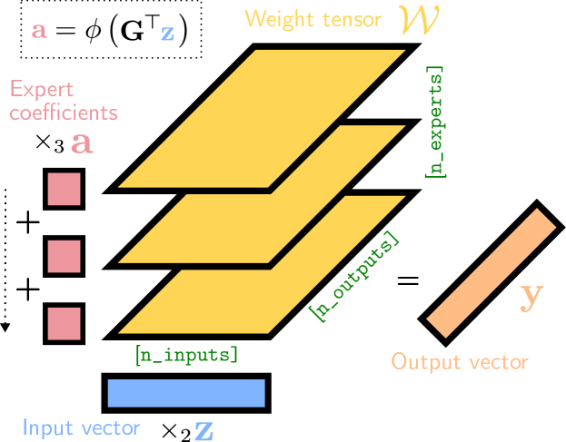
Figure 1: Illustration of a single-hierarchy ($E=1$) MMoE layer’s (unfactorized) forward pass as a series of tensor contractions. The experts’ weight matrices are visualized as $2$D horizontal slices in yellow, which are matrix-multiplied with the input vector and summed (weighted by the expert coefficients in red).

Table 1: A guide to decomposition choice for MMoE layers, based on efficiency. In the right-most column, a numerical estimation of the number of FLOPs is made for CLIP ViT-B-32 models with $512$-expert MMoE final layers for ImageNET1k.

	Param-efficient	Param-efficient		Scales well		Estimated # FLOPs	Estimated # FLOPs
	(medium $N$)	(large $N$)	RAM-efficient	with hierarchies	# Parameters	(algebraic)	(numerical)
Soft MoE					$OIN$	$OIN$	$393$M
CPMMoE					$R(O+I+N)$	$R(O+I+N)$	$1.1$M
TuckerMMoE					$R_{I}I+R_{N}N+R_{O}O+R_{O}R_{I}R_{N}$	$R_{I}I+R_{O}R_{I}R_{N}+R_{N}N+R_{O}R_{N}+R_{O}O$	$2.4$M
T*MMoE					$R_{1}OR_{2}+R_{2}IR_{3}+R_{3}NR_{1}$	$R_{2}IR_{3}+R_{3}NR_{1}+R_{1}R_{2}R_{3}+R_{1}R_{2}O$	$2.6$M

CPMMoE

If we assume the weight tensor has low-rank CP structure (Hitchcock, 1927; Carroll & Chang, 1970) of rank $R$, we have $\mathcal{W}=\sum_{r=1}^{R}\mathbf{g}^{(1)}_{r}\circ\mathbf{g}^{(2)}_{r}\circ\mathbf{g}^{(3)}_{r}$ (a sum of $R$ outer products), with factor matrices $\mathbf{G}^{(1)}\in\mathbb{R}^{R\times O},\mathbf{G}^{(2)}\in\mathbb{R}^{R\times I},\mathbf{G}^{(3)}\in\mathbb{R}^{R\times N}$. The CPMMoE layer’s forward pass can be computed entirely in factorized form without ever materializing the full tensor as

$$\mathbf{y} =\left(\sum_{r=1}^{R}\mathbf{g}^{(1)}_{r}\circ\mathbf{g}^{(2)}_{r}\circ\mathbf{g}^{(3)}_{r}\right)\times_{2}\mathbf{z}\times_{3}\mathbf{a}$$

$$=\sum_{r=1}^{R}\mathbf{g}^{(1)}_{r}\big{(}\sum_{n,i}g_{ri}^{(2)}g_{rn}^{(3)}z_{i}a_{n}\big{)}$$

$$=\sum_{r=1}^{R}\mathbf{g}^{(1)}_{r}\big{(}{\mathbf{G}^{(2)}}^{\top}\mathbf{z}\big{)}_{r}\cdot\big{(}{\mathbf{G}^{(3)}}^{\top}\mathbf{a}\big{)}_{r}\in\mathbb{R}^{O},$$ (2)

with Equation 2 being analogous to the fast computation in Babiloni et al. (2023), only here the operations of combining the weights and producing the outputs can be expressed in a single step. We adopt the convention of counting fused multiply-adds as one operation to be consistent with popular PyTorch libraries when estimating FLOPs. Whilst the original naive CPMMoE forward pass has a FLOP count of $OIN$, the fast computation above has just $R(O+I+N)$ (the same number of factorized layer parameters). With moderate values of both $R$ and $N$, the layer becomes significantly more resource-efficient than vanilla MMoEs. When $N$ increases significantly, however, alternative decomposition choices can offer even better efficiency.

TuckerMMoE

One such alternative is the Tucker decomposition (Tucker, 1966; Hitchcock, 1927). A Tucker-structured MMoE weight tensor can be written as $\mathcal{W}=\mathcal{Z}\times_{1}\mathbf{G}^{(1)}\times_{2}\mathbf{G}^{(2)}\times_{3}\mathbf{G}^{(3)}$, where $\mathcal{Z}\in\mathcal{R}^{R_{O}\times R_{I}\times R_{N}}$ is the so-called ‘core tensor’ and $\mathbf{G}_{1}\in\mathbb{R}^{O\times R_{O}},\mathbf{G}_{2}\in\mathbb{R}^{I\times R_{I}},\mathbf{G}_{3}\in\mathbb{R}^{N\times R_{N}}$ are the ‘factor matrices’ for the tensor’s three modes. Using Property 2 of the mode-$n$ product in De Lathauwer et al. (2000), a TuckerMMoE forward pass can be computed in factorized form as

$$\mathbf{y} =\big{(}\mathcal{Z}\times_{1}\mathbf{G}^{(1)}\times_{2}\mathbf{G}^{(2)}\times_{3}\mathbf{G}^{(3)}\big{)}\times_{2}\mathbf{z}\times_{3}\mathbf{a}$$

$$=\mathcal{Z}\times_{2}\mathbf{z}\mathbf{G}^{(2)}\times_{3}\mathbf{a}\mathbf{G}^{(3)}\times_{1}\mathbf{G}^{(1)}\in\mathbb{R}^{O}.$$ (3)

Contracting over the modes in this order requires a total of only $R_{I}I+R_{O}R_{I}R_{N}+R_{N}N+R_{O}R_{N}+R_{O}O$ FLOPs. An attractive property here is one can alter mode-$i$ specific ranks $R_{i}$ as desired individually to greatly reduce both FLOPs and parameter count alike–even when $N$ increases drastically. However, contracting over the $R_{O}R_{I}R_{N}$-dimensional core tensor with a batch of inputs can be RAM-intensive, and does not scale particularly well to additional hierarchies (see Appendix C).

TTMMoE and TRMMoE

We propose two final MMoE model variants based on the Tensor Train (Oseledets, 2011) (TT) and Tensor Ring (Zhao et al., 2016) (TR) decompositions that address the two aforementioned drawbacks of TuckerMMoEs. In TT/TR format, $\mathcal{W}\in\mathbb{R}^{O\times I\times N}$ has three factor tensors: $\mathcal{G}_{1}\in\mathbb{R}^{R_{1}\times O\times R_{2}}$, $\mathcal{G}_{2}\in\mathbb{R}^{R_{2}\times I\times R_{3}}$, $\mathcal{G}_{3}\in\mathbb{R}^{R_{3}\times N\times R_{4}}$, where $R_{i}$ are the manually chosen ranks (with $R_{1}=R_{4}$ for TR and $R_{1}=R_{4}=1$ for TT through the ‘boundary conditions’). The weight tensor’s elements are given by: $\mathcal{W}(o,i,n)=\text{tr}\big{(}{\mathcal{G}_{1}(:,o,:)}{\mathcal{G}_{2}(:,i,:)}{\mathcal{G}_{3}(:,n,:)}\big{)}$, and thus both a TTMMoE and TRMMoE forward pass can be computed solely through operating on its factor tensors as:

$$\mathbf{y} =\sum_{n,i}\mathcal{W}(:,i,n)z_{i}a_{n}$$

$$=\sum_{\mathclap{n,i,r_{1},r_{2},r_{3}}}\mathcal{G}_{1}(r_{1},:,r_{2})\mathcal{G}_{2}(r_{2},i,r_{3})\mathcal{G}_{3}(r_{3},n,r_{1})z_{i}a_{n}$$

$$=\sum_{r=1}^{R_{1}}\bigg{(}\underbrace{\mathcal{G}_{1}\times_{3}\underbrace{\big{(}\mathcal{G}_{2}\times_{2}\mathbf{z}\big{)}\big{(}\mathcal{G}_{3}\times_{2}\mathbf{a}\big{)}}_{R_{2}\times R_{1}}}_{R_{1}\times O\times R_{1}}\bigg{)}_{r:r}\in\mathbb{R}^{O}.$$ (4)

The fast forward passes of both T*MMoE models consequently have a modified FLOP count of $R_{2}IR_{3}+R_{3}NR_{1}+R_{1}R_{2}R_{3}+R_{1}R_{2}O$, with just $R_{1}OR_{2}+R_{2}IR_{3}+R_{3}NR_{1}$ parameters.

3.1.2 Bilinear MMoEs recover MoEs as a special case

MMoE layers recover (linear) MoE layers (Shazeer et al., 2017) as a special case. Assume a non-factorized MMoE layer with one level of hierarchy. Through the definition of the mode-$n$ product, we can write the output vector $\mathbf{y}\in\mathbb{R}^{O}$ elementwise as

$$\mathbf{y} =\mathcal{W}\times_{2}\mathbf{z}\times_{3}\mathbf{a}=\sum_{n}\sum_{i}a_{n}\mathbf{w}_{:in}z_{i}=\sum_{n}a_{n}(\mathbf{W}_{::n}\mathbf{z}),$$

which is precisely the formulation of the dynamic perceptron in Chen et al. (2020) and linear variant of the MoE of Shazeer et al. (2017). The re-formulation above sheds further light on MoEs more generally, through its connection to the mode-$n$ product: with each output element computed as $y_{o}=\mathbf{a}^{\top}\mathbf{W}_{o}\mathbf{z}$, linear MoEs can be seen as bilinear layers.

4 Experiments

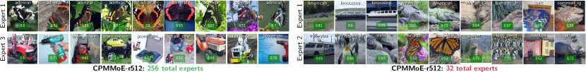
Figure 2: Visual comparison to CPMMoE layers with $256$ (left) and $32$ (right) total experts. Each row displays randomly selected images processed (with coefficient $\geq 0.5$) by the first few experts for the two models. We highlight the lack of a singular visual theme in the images processed by individual experts with the model with low total expert count (and vice versa).

We start in Section 4.1 by presenting both qualitative and quantitative experiments validating that the experts learn to perform subtasks of classifying different semantic clusters of the input data in a modular manner. In Section 4.2 we demonstrate one practical benefit of the learned modularity–showing how expert-conditional re-writing can correct for specific demographic bias in CelebA attribute classification. Finally, we compare the MMoE’s performance to linear and parameter-matched linear layers in Section 4.3. We make comparisons between MMoE configurations and rank choices throughout the main paper where space permits and include additional ablation studies in Appendix E. A particular MMoE configuration is specified with the format {model}-r{rank}-e{n_experts}. In all our experiments in the main paper, we use a single level of experts–please see Appendix C for experiments with up to $4$ levels of hierarchy in MMoEs fine-tuned on ImageNET1k, where layers with 2 or 3 levels of hierarchy achieve the highest accuracy across all MMoE variants. All results presented in this section are the average of 10 runs with different random seeds (5 runs for all experiments on ImageNET1k).

Implementation details

For all MMoE layers we first batch-normalize the expert coefficients pre-activation, i.e. $\mathbf{a}=\phi(\mathbf{G}^{\top}\mathbf{z})=\mathrm{entmax}(\mathrm{BN}(\mathbf{G}^{\top}\mathbf{z}))$. We find this balances the expert load sufficiently well without need for any load-balancing losses.

4.1 Expert modularity: visualization & intervention

Here we aim to provide both qualitative (through visualization) and quantitative evidence (through intervention) that MMoE layer image classifiers perform the computation responsible for classifying particular ‘semantic groups’ of ImageNET1k classes. Furthermore, we show that increasing the total number of experts in an MMoE layer leads to increasingly modular, category-specific experts.

4.1.1 Qualitative results

Concretely, we fine-tune CLIP ViT-B-32 models on ImageNET1k (Deng et al., 2009) with CPMMoE-r512 final classification layers, following the experimental setup in Ilharco et al. (2022, 2023).

Using both 32 and 256 total experts, we first show random examples in Figure 2 of images processed (with expert coefficient $\geq 0.5$) by the first experts as they appear numerically. The class labels and expert coefficients are overlaid in white and green text respectively. Using only a modest number of experts (e.g. 32) appears to produce polysemantic experts–with some processing many unrelated classes of images (e.g. ‘gators’, ‘limos’, and a ‘quilt’ for Expert 1 on the right). On the other hand, using a much larger number of total experts appears to successfully yield more specialization, with many processing images of either the same class label or broader category. Please see Figure 7 in the Appendix for many more random images for the first $10$ experts per model to observe this same trend more generally, and Figure 8 for even finer-grained specialism with $2048$-expert MMoE layers. We highlight that MMoE’s factorized forward passes are crucial in making it feasible to conduct computations involving such a large number of experts facilitating this level of specialization. The $2048$-expert layer, for example, requires $1.2\mathrm{B}$ parameters and FLOPs in a Soft MoE, whilst only $1.9\mathrm{M}$ in the CPMMoE.

The qualitative evidence here hints at the potential of a prominent benefit to scaling up the number of experts–the larger the total number of experts, the more granular the clusters of processed images appear to be. Such subjective interpretations alone are hypotheses, rather than conclusions however (Räuker et al., 2023). The results in Figure 2 give us an intuitive explanation of the function of the first few experts, but do not show that they contribute causally (Elazar et al., 2021; Ravfogel et al., 2021; Meng et al., 2022) to the subtask of classifying human-understandable subgroups of data (Rudin, 2019; Casper, 2023). We accordingly turn in the next two sections to quantifying the experts’ functional role in the network in two different ways: first through interventions, and second through expert re-writing.

4.1.2 Quantitative results

One major difficulty in quantifying expert monosemanticity is the absence of ground-truth labels for interpretable features of the input one may be interested in (e.g. an animal having a furry coat, or big ears). Despite this, we can measure the effect an expert has on the per-class accuracy as an imperfect proxy (Hod et al., 2021). Here, we aim to investigate the causal role the experts play in classifying particular subgroups in the test set. In particular, following the causal intervention protocol of Elazar et al. (2021), we ask the specific counterfactual question about solely each expert $n$ in turn: “had expert $n$’s weight matrix $\mathbf{W}_{::n}$ not contributed its computation, would the network’s test-set accuracy for class $c$ have dropped?”

Practically speaking, given a network fine-tuned with an MMoE layer, we achieve this by intervening in the forward pass by zeroing the $n^{\text{th}}$ expert’s weight matrix $\mathbf{W}_{::n}:=\mathbf{0}$, leaving every other aspect of the forward pass completely untouched. Let the elements of $\mathbf{y},\hat{\mathbf{y}}^{(n)}\in\mathbb{R}^{C}$ denote the test set accuracy for the $C=1000$ ImageNET1k classes, pre- and post-intervention of expert $n$ respectively. We collect the normalized difference to per-class accuracy in the vector $\mathbf{d}^{(n)}$, whose elements are given by $d^{(n)}_{c}=(y_{c}-\hat{y}^{(n)}_{c})/y_{c}$. At the two extremes, when the full network’s accuracy for class $c$ drops completely from $y_{c}$ to $0$ upon manually excluding expert $n$’s computation we get $d^{(n)}_{c}=1$, whilst $d^{(n)}_{c}=0$ means the absence of the subcomputation did not change class $c$’s test set accuracy at all. We thus measure the class-level polysemanticity of expert $n$ as the distance between the difference vector and the one-hot vector:

$$p^{(n)}=||\mathbf{d}^{(n)}-\mathds{1}^{(n)}||_{2},$$ (5)

where index $\mathrm{argmax}_{c}(d_{c}^{(n)})$ of $\mathds{1}^{(n)}$ has a value of $1$ (and values of $0$ everywhere else). This encodes the signature of a perfectly class-level monosemantic expert, for which all accuracy for a single class alone is lost in the counterfactual scenario in which the expert $n$ did not contribute.

We plot in Figure 3 the average expert polysemanticity $p^{(n)}$ for all experts with non-zero difference vectors, observing a steady drop in its value as $N$ increases from $32$ to $1024$ total experts. In other words, increasing $N$ leads to individual experts increasingly responsible for a single subtask: classifying all inputs of just one class.

We refer readers to the bar plots of the values of $\mathbf{d}^{(n)}$ (the per-class accuracy changes) in Figures 5 and 6, where this trend is observable through mass concentrated on increasingly fewer class labels as the number of experts increases.

4.2 Expert re-writing: conditional bias correction

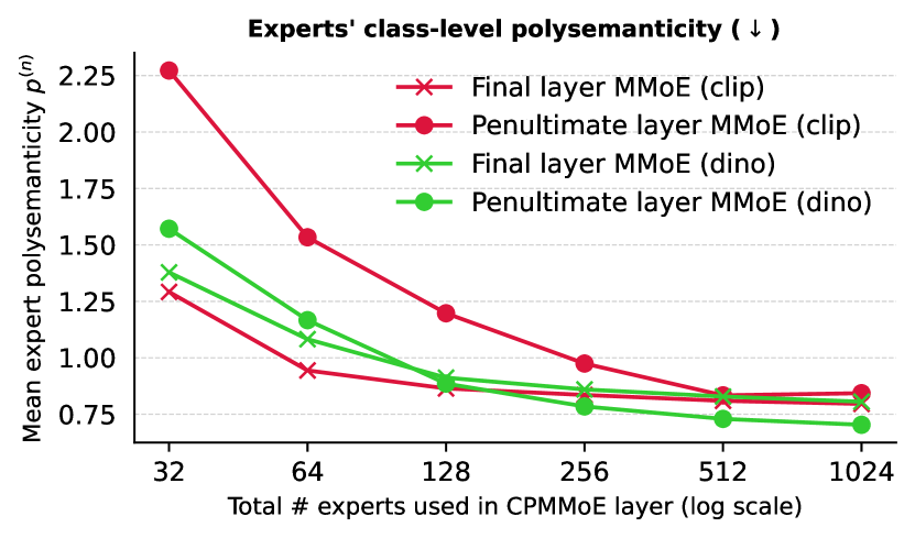
Figure 3: Mean expert class-level polysemanticity of Equation 5 ($\downarrow$) as a function of the total number of experts. Results are shown for both CLIP ViT-B-32 and DINO models fine-tuned on ImageNET1k with CPMMoE-r512 layers.

Table 2: Fairness metrics and ‘model re-writing score’ (MRS) for baseline models and after applying various fairness techniques in the literature, for the two experiments on CelebA. A CPMMoE-r512-e128 model is used as the final layer (please zoom for detail).

	(a) Bias towards ‘Old females’ for ‘Age’ prediction head							(b) Bias towards ‘Blond males’ for ‘Blond Hair’ prediction head
			(Hardt et al., 2016)	(Wang & Deng, 2020)	(Lahoti et al., 2020)						(Hardt et al., 2016)	(Wang & Deng, 2020)	(Lahoti et al., 2020)
	MRS ($\uparrow$)	Target subpop. acc. ($\uparrow$)	Equality of opp. ($\downarrow$)	STD bias ($\downarrow$)	Subpop. Max-Min ($\uparrow$)	Test set acc. ($\uparrow$)			MRS ($\uparrow$)	Target subpop. acc. ($\uparrow$)	Equality of opp. ($\downarrow$)	STD bias ($\downarrow$)	Subpop. Max-Min ($\uparrow$)	Test set acc. ($\uparrow$)	# Params
Linear	-	0.516	0.226	0.185	0.516	88.944			-	0.346	0.534	0.263	0.346	95.833	30.7K
HighRankLinear	-	0.513	0.228	0.186	0.513	88.920			-	0.353	0.529	0.260	0.353	95.831	827K
CPMMoE	-	0.555	0.197	0.167	0.555	89.048			-	0.409	0.476	0.236	0.409	95.893	578K
+ oversample	-	0.669	0.086	0.120	0.669	89.009			-	0.655	0.226	0.131	0.655	95.750	578K
+ adv. debias (Alvi et al., 2018)	-	0.424	0.274	0.226	0.424	87.785			-	0.193	0.630	0.325	0.193	95.031	579K
+ blind thresh. (Hardt et al., 2016)	-0.22	0.843	0.082	0.084	0.700	83.369			0.21	0.843	0.139	0.063	0.841	92.447	578K
+ expert thresholding (ours)	0.13	0.866	0.097	0.066	0.756	84.650			0.39	0.847	0.051	0.048	0.846	94.895	578K

We further validate the modular expert hypothesis and simultaneously provide a concrete example of its usefulness by correcting demographic bias in attribute classification. Classifiers trained to minimize the standard binary cross-entropy loss often exhibit poor performance for demographic subpopulations with low support (Buolamwini & Gebru, 2018; Gebru et al., 2021). By identifying which combination of experts is responsible for processing target subpopulations, we show how one can straightforwardly manually correct mispredictions in a targeted way–without any re-training.

We focus on mitigating bias towards two low-support subpopulations in models with MMoE final layers fine-tuned on CelebA (Liu et al., 2015): (a) bias towards images labeled as ‘old females’ for age prediction (Jain et al., 2023), and (b) bias towards images labeled as ‘blond males’ for blond hair prediction (Mao et al., 2023). Concretely, we train a multi-label MMoE final layer for the 40 binary attributes in CelebA, jointly optimizing a pre-trained CLIP ViT-B-32 model (Radford et al., 2021) backbone, again following the experimental setup in Ilharco et al. (2022, 2023). We use $N:=128$ experts, thus the MMoE weight tensor for the classification layer is implicitly of dimension $\mathcal{W}\in\mathbb{R}^{40\times 769\times 128}$ (where $768+1$ is the dimension of CLIP’s cls token’s feature vector plus an extra dimension for the experts’ bias terms).

Experimental setup

Let $C$ be a set collecting the expert coefficients $\mathbf{a}\in\mathbb{R}^{N}$ from forward passes of the training images belonging to the target subpopulation. We evaluate the subpopulation’s mean expert coefficients $\mathbf{\bar{a}}=1/|C|\sum_{\mathbf{a}\in C}\mathbf{a}\in\mathbb{R}^{N}$, proposing to manually re-write the output of this expert combination. We modify the layer’s forward pass for the $o^{\text{th}}$ output head for attribute of interest (e.g. ‘blond hair’) as:

$$y_{o}=(\mathcal{W}\times_{2}\mathbf{z}\times_{3}\mathbf{a})_{o}+\lambda\mathbf{\bar{a}}^{\top}\mathbf{a}.$$ (6)

Here, the term $\lambda\mathbf{\bar{a}}\in\mathbb{R}^{N}$ specifies, for each expert, how much to increase/decrease the logits for attribute $o$, with $\lambda$ being a scaling hyperparameter. Taking the dot product with an input image’s expert coefficients $\mathbf{a}$ applies the relevant experts’ correction terms (in the same way it selects a subset of the most relevant experts’ weight matrices).

4.2.1 Experimental results

Fairness metrics

First, we report a range of standard fairness metrics for both the model rewriting and networks trained with existing techniques (that aim to mitigate demographic bias without requiring images’ sensitive attribute value at test time). These are shown in Table 2 for the two different experiments on CelebA, where the proposed intervention outperforms baseline alternative methods in the majority of settings. Please see Appendix G for details about the baseline methods and fairness metrics used, and further discussion of results.

Model re-writing score

Table 3: Test set accuracy fine-tuning a CLIP vit_base_patch32 model. Average results are reported over $10$ random seeds ($5$ for ImageNET1k). Comparisons are made to regular linear layers and CPMMoE-r512-e128 parameter-matched (p.m.) linear layers.

	CIFAR100		Caltech256		Caltech101		Food101		OxfordIIITPet		CelebA		ImageNET1k
	Accuracy	# Params	Accuracy	# Params	Accuracy	# Params	Accuracy	# Params	Accuracy	# Params	Accuracy	# Params	Accuracy	# Params
Linear	$87.62\pm 0.16$	76900	$89.75\pm 0.50$	197633	$\textbf{96.54}\pm\textbf{0.59}$	78438	$87.07\pm 0.06$	77669	$89.57\pm 0.49$	28453	$92.22\pm 0.02$	30760	$72.97\pm 0.07$	769000
Linear (p.m.)	$87.23\pm 0.25$	888932	$88.85\pm 0.57$	1049857	$96.03\pm 0.67$	890982	$86.54\pm 0.12$	889957	$88.02\pm 0.45$	824357	$92.18\pm 0.01$	827432	$72.28\pm 0.14$	1811432
CPMMoE	$\textbf{88.11}\pm\textbf{0.15}$	608768	$\textbf{90.46}\pm\textbf{0.57}$	689152	$96.44\pm 0.77$	609792	$\textbf{88.27}\pm\textbf{0.10}$	609280	$\textbf{90.31}\pm\textbf{0.52}$	576512	$\textbf{92.24}\pm\textbf{0.02}$	578048	$\textbf{73.78}\pm\textbf{0.07}$	1069568

The fairness metrics above are also impacted by the remaining subpopulations’ existing accuracy, however. A precise model re-write should bring a large improvement in accuracy to the target subpopulation (e.g. young males), whilst affecting the accuracy for the remaining subpopulations’ (e.g. females, old males) as little as possible. We thus propose to further quantify this more directly with a model re-writing score. We take this to be the positive change to the target subpopulation’s test set accuracy, minus the sum of the absolute changes to the test set accuracy for the remaining subpopulations. Similarly to the expert intervention experiments, let vectors $\mathbf{y},\hat{\mathbf{y}}\in\mathbb{R}^{A}$ contain in their elements the test-set accuracy for $A$ different demographic subpopulations, before and after intervention respectively. For the subpopulation $A$ of interest, the model re-writing score (MRS) is given by: $\text{MRS}(\mathbf{y},\hat{\mathbf{y}},a)=(\hat{y}_{a}-y_{a})-\sum_{\begin{subarray}{c}i=1\\ i\neq a\end{subarray}}^{A}|\hat{y}_{i}-y_{i}|.$ A perfect re-write yields the highest MRS of $1-y_{a}$ when all instances of the target subpopulation in the test set have had their classifications corrected, with no effect on any of the other subpopulations. We compare the proposed expert-conditional re-writing of Equation 6 with a static, unconditional fairness threshold (which can be seen as a manual, ‘protected attribute-blind’ variant of the method in Hardt et al. (2016)). The attribute-blind unconditional thresholding is achieved by setting $\bar{\mathbf{a}}$ to a vector of $1$s, and $\lambda:=2.5$. The results for CPMMoEs are included in Table 2, with full results and ablations in the Appendix. The full subpopulation accuracies before and after re-writing, vs the baseline are also shown for all MMoE variants in Appendix H. As can be seen clearly, expert-conditional logit correction is far more precise than unconditional fairness thresholding thanks to the expert specialism.

4.3 MMoE performance

Finally, we aim to substantiate the claim that MMoE final-layer image classification accuracy is competitive with parameter-matched linear layer alternatives. To this end, we fine-tune a CLIP-ViT-B32 model on $7$ popular image datasets, again following the experimental configuration of Ilharco et al. (2022, 2023). We compare with the standard $\mathbf{y}=\mathbf{Wx}+\mathbf{b}$ linear classifier, and ‘high-rank’ counterpart of the form: $\mathbf{y}=\mathbf{W}_{1}^{\top}\mathbf{W}_{2}\mathbf{x}+\mathbf{b}$, where $\mathbf{W}_{1}\in\mathbb{R}^{R\times C},\mathbf{W}_{2}\in\mathbb{R}^{R\times I}$. We scale up the value of $R$ such that the layer has at least as many parameters as the MMoE layer compared.

The CLIP fine-tuning comparisons are shown in Table 3, where we see the MMoE performance is competitive with the linear counterpart on many datasets. Please see Appendix F for many additional results on DINO (Caron et al., 2021), and comparisons with all MMoE variants when the number of experts is varied from $2$ all the way to $16$k. Experiments with multiple levels of hierarchy are also included in Appendix C.

5 Conclusion

In this paper, we introduced the Multilinear Mixture of Experts layer (MMoE). We demonstrated how MMoE layers facilitate efficient computation with up to thousands of experts. Further, we showed how increasing MMoE’s total expert count leads to more specialized subcomputation within each, focusing on vision. MMoE layers do not suffer from the same problems as existing Sparse MoEs, yet are often orders of magnitude cheaper than Soft MoEs. As a further practical example of MMoE’s task decomposition, we illustrate how manual guided edits can be made to correct bias towards demographic subpopulations in fine-tuned foundation models. We believe MMoE layers constitute an important step towards facilitating increasingly performant models that do not trade-off fairness/interpretability for accuracy.

Limitations

of the MMoE layer come in a few forms. Firstly, it is important to state again that our quantitative evaluation only captures expert behavior on the test set, not out-of-domain data (Casper, 2023; Bolukbasi et al., 2021). Future work could explore how well MMoEs generalize under domain shift and their application to NLP tasks.

6 Impact Statement

This paper presents work whose goal is to advance the field of interpretable machine learning. Our goal is not to improve model capabilities but rather an orthogonal one of designing more interpretable and controllable architectures. As with many work with an interpretability focus, however, the MMoE layer could nonetheless facilitate the further development of SOTA models through its more expressive computation. We thus encourage the development of further guardrails against potentially harmful dual-uses of such technology.

Appendix A Full MMoE model derivations

In the main paper, the fast forward passes are derived for a single level of expert hierarchy for ease of presentation. Here, we derive the fast forward passes in full for MMoE layers in their most general form with $E$ levels of expert hierarchy. We first recall the definition of the $E$-level MMoE layer from Section 3.1 in the main paper: given input $\mathbf{z}\in\mathbb{R}^{I}$, an MMoE layer is parameterized by weight tensor $\mathcal{W}\in\mathbb{R}^{O\times I\times N_{1}\times\ldots\times N_{E}}$ and expert gating parameters $\{\mathbf{G}_{e}\in\mathbb{R}^{I\times N_{e}}\}_{e=1}^{E}$. The explicit, unfactorized forward pass is given by:

$$\mathbf{a}_{e} =\phi(\mathbf{G}_{e}^{\top}\mathbf{z})\in\mathbb{R}^{N_{e}},\quad\forall e\in\{1,\ldots,E\},$$

$$\mathbf{y} =\mathcal{W}\times_{2}\mathbf{z}\times_{3}\mathbf{a}_{1}\times_{4}\ldots\times_{E+2}\mathbf{a}_{E}\in\mathbb{R}^{O}.$$

With expert coefficients $\{\mathbf{a}_{e}\in\mathbb{R}^{N_{e}}\}_{e=1}^{E}$, the factorized forward passes of the full hierarchical MMoE layers are given as follows:

CPMMoE

The full CPMMoE model of rank $R$ has an implicit weight tensor $\mathcal{W}=\sum_{r=1}^{R}\mathbf{g}^{(1)}_{r}\circ\mathbf{g}^{(2)}_{r}\circ\mathbf{g}^{(3)}_{r}\circ\cdots\circ\mathbf{g}^{(E+2)}_{r}\in\mathbb{R}^{O\times I\times N_{1}\times\cdots\times N_{E}}$, with factor matrices $\mathbf{G}^{(1)}\in\mathbb{R}^{R\times O},\mathbf{G}^{(2)}\in\mathbb{R}^{R\times I},\mathbf{G}^{(3)}\in\mathbb{R}^{R\times N_{1}},\ldots,\mathbf{G}^{(E+2)}\in\mathbb{R}^{R\times N_{E}}$. The implicit, factorized forward pass is given by:

$$\mathbf{y} =\left(\sum_{r=1}^{R}\mathbf{g}^{(1)}_{r}\circ\mathbf{g}^{(2)}_{r}\circ\mathbf{g}^{(3)}_{r}\circ\cdots\circ\mathbf{g}^{(E+2)}_{r}\right)\times_{2}\mathbf{z}\times_{3}\mathbf{a}_{1}\times_{4}\ldots\times_{E+2}\mathbf{a}_{E}$$

$$=\sum_{r=1}^{R}\mathbf{g}^{(1)}_{r}\big{(}\sum_{{n_{1}},\ldots,{n_{E}},i}g_{ri}^{(2)}z_{i}g_{rn_{1}}^{(3)}a_{1_{n_{1}}}\cdots g_{r{n_{E}}}^{(E+2)}a_{E_{n_{E}}}\big{)}$$

$$=\sum_{r=1}^{R}\mathbf{g}^{(1)}_{r}\big{(}{\mathbf{G}^{(2)}}^{\top}\mathbf{z}\big{)}_{r}\cdot\big{(}{\mathbf{G}^{(3)}}^{\top}\mathbf{a}_{1}\big{)}_{r}\cdots\big{(}{\mathbf{G}^{(E+2)}}^{\top}\mathbf{a}_{E}\big{)}_{r}\in\mathbb{R}^{O}.$$ (7)

TuckerMMoE

The full TuckerMMoE model has an implicit weight tensor $\mathcal{W}=\mathcal{Z}\times_{1}\mathbf{G}^{(1)}\times_{2}\mathbf{G}^{(2)}\times_{3}\mathbf{G}^{(3)}\times_{4}\cdots\times_{E+2}\mathbf{G}^{(E+2)}\in\mathbb{R}^{O\times I\times N_{1}\times\cdots\times N_{E}}$, where $\mathcal{Z}\in\mathcal{R}^{R_{O}\times R_{I}\times R_{N_{1}}\times\cdots\times R_{N_{E}}}$ is the so-called ‘core tensor’ and $\mathbf{G}_{1}\in\mathbb{R}^{O\times R_{O}},\mathbf{G}_{2}\in\mathbb{R}^{I\times R_{I}},\mathbf{G}_{3}\in\mathbb{R}^{N_{1}\times R_{N_{1}}},\ldots,\mathbf{G}_{E+2}\in\mathbb{R}^{{N_{E}}\times R_{N_{E}}}$ are the ‘factor matrices’ for the tensor’s $E+2$ modes. The implicit, factorized forward pass is given by:

$$\mathbf{y} =\big{(}\mathcal{Z}\times_{1}\mathbf{G}^{(1)}\times_{2}\mathbf{G}^{(2)}\times_{3}\mathbf{G}^{(3)}\times_{4}\cdots\times_{E+2}\mathbf{G}^{(E+2)}\big{)}\times_{2}\mathbf{z}\times_{3}\mathbf{a}_{1}\times_{4}\cdots\times_{E+2}\mathbf{a}_{E}$$

$$=\mathcal{Z}\times_{1}\mathbf{G}^{(1)}\times_{2}\mathbf{z}\mathbf{G}^{(2)}\times_{3}\mathbf{a}_{1}\mathbf{G}^{(3)}\times_{4}\cdots\times_{E+2}\mathbf{a}_{E}\mathbf{G}^{(E+2)}$$

$$=\mathcal{Z}\times_{2}\mathbf{z}\mathbf{G}^{(2)}\times_{3}\mathbf{a}_{1}\mathbf{G}^{(3)}\times_{4}\cdots\times_{E+2}\mathbf{a}_{E}\mathbf{G}^{(E+2)}\times_{1}\mathbf{G}^{(1)}\in\mathbb{R}^{O}.$$ (8)

TTMMoE and TRMMoE

In TT/TR format, $\mathcal{W}\in\mathbb{R}^{O\times I\times N_{1}\times\cdots\times N_{E}}$ has $E+2$ factor tensors: $\mathcal{G}_{1}\in\mathbb{R}^{R_{1}\times O\times R_{2}}$, $\mathcal{G}_{2}\in\mathbb{R}^{R_{2}\times I\times R_{3}}$, $\mathcal{G}_{3}\in\mathbb{R}^{R_{3}\times N_{1}\times R_{4}},\ldots,\mathcal{G}_{E+2}\in\mathbb{R}^{R_{E+2}\times N_{E}\times R_{E+3}}$, where $R_{i}$ are the manually chosen ranks (with $R_{1}=R_{E+3}$ for TR and $R_{1}=R_{E+3}=1$ for TT through the ‘boundary conditions’). The weight tensor’s elements are given by:

$$\mathcal{W}(o,i,n_{1},\ldots,n_{E})=\text{tr}\big{(}{\mathcal{G}_{1}(:,o,:)}{\mathcal{G}_{2}(:,i,:)}{\mathcal{G}_{3}(:,n_{1},:)}\cdots{\mathcal{G}_{E+2}(:,n_{E},:)}\big{)}.$$

The implicit, factorized forward pass is given by:

$$\mathbf{y} =\sum_{i}\sum_{n_{1},\ldots,n_{E}}\mathcal{W}(:,i,n_{1},\ldots,n_{E})z_{i}a_{n_{1}}\cdots a_{n_{E}}$$

$$=\sum_{i}\sum_{n_{1},\ldots,n_{E}}\sum_{r_{1},\ldots,r_{E+3}}{\mathcal{G}_{1}(r_{1},:,r_{2})}{\mathcal{G}_{2}(r_{2},i,r_{3})}{\mathcal{G}_{3}(r_{3},n_{1},r_{4})}\cdots{\mathcal{G}_{E+2}(r_{E+2},n_{E},r_{E+3})}z_{i}{a_{n_{1}}}\cdots{a_{n_{E}}}$$

$$=\sum_{r=1}^{R_{1}}\bigg{(}\underbrace{\mathcal{G}_{1}\times_{3}\underbrace{\big{(}\mathcal{G}_{2}\times_{2}\mathbf{z}\big{)}\big{(}\mathcal{G}_{3}\times_{2}\mathbf{a}_{1}\big{)}\cdots\big{(}\mathcal{G}_{E+2}\times_{2}\mathbf{a}_{E}\big{)}}_{R_{2}\times R_{1}}}_{R_{1}\times O\times R_{1}}\bigg{)}_{r:r}\in\mathbb{R}^{O}.$$ (9)

Appendix B MMoE implementations

Next we detail how to implement the forward passes of the 4 MMoE models in a batch-wise manner with PyTorch and einops’ (Rogozhnikov, 2022) einsum. We present these implementations in as readable and concise a manner as possible for intuition but note that Tucker+TR implementations can be made more RAM-efficient in PyTorch by following the order of operations in the main paper (please see the supporting MMoE.py model code)–contracting over specific modes of the factor tensors at a time, rather than all together in a single big einsum.

CPMMoE

The CPMMoE forward pass (and two-level hierarchical CPMMoE with an additional factor matrix) can be implemented with: # CPMMoE (r=CP rank, b=batch_dim, i=input_dim, o=output_dim, n*=expert_dims) y = einsum(G1, z@G2.T, a1@G3.T, ’r o, b r, b r -¿ b o’)

# A two-level hierarchical CPMMoE y = einsum(G1, z@G2.T, a1@G3.T, a2@G4.T, ’r o, b r, b r, b r -¿ b o’)

TuckerMMoE

Assuming core tensor and factor matrices of appropriate size, the TuckerMMoE forward pass can be implemented as below. Additional hierarchies of experts with TuckerMMoEs can be implemented by appending another ‘expert mode’ to the core tensor, and introducing another factor matrix, e.g.: # TuckerMMoE (r*=tucker ranks, b=batch_dim, i=input_dim, o=output_dim, n*=expert_dims) y = einsum(Z, G1, z@G2, a1@G3, ’ro ri rn1, o ro, b ri, b rn1 -¿ b o’)

# A two-level hierarchical TuckerMMoE, assuming appropriate new dimensions for Z y = einsum(Z, G1, z@G2, a1@G3, a2@G4, ’ro ri rn1 rn2, o ro, b ri, b rn1, b rn2 -¿ b o’)

TTMMoE and TRMMoE

Both a TTMMoE and TRMMoE’s (and two-level hierarchical version with an additional TT/TR-core) can be implemented with:

# TT/TRMMoE (r*=TT/TR ranks, b=batch_dim, i=input_dim, o=output_dim, n*=expert_dims) # note: r1 = 1 for a TTMMoE f1 = einsum(z, G2, ’b i, r2 i r3 -¿ b r2 r3’) # batched mode-2 tensor-vector product f2 = einsum(a1, G3, ’b n1, r3 n1 r1 -¿ b r3 r1’) # batched mode-2 tensor-vector product

y = einsum(G1, f1, f2, ’r1 o r2, b r2 r3, b r3 r1 -¿ b o’)

# A two-level hierarchical TT/TRMMoE, assuming appropriate new dimensions for Gi # note: r1 = 1 for a TTMMoE f1 = einsum(z, G2, ’b i, r2 i r3 -¿ b r2 r3’) # batched mode-2 tensor-vector product f2 = einsum(a1, G3, ’b n1, r3 n1 r4 -¿ b r3 r4’) # batched mode-2 tensor-vector product f3 = einsum(a2, G4, ’b n2, r4 n2 r1 -¿ b r4 r1’) # batched mode-2 tensor-vector product

y = einsum(G1, f1, f2, f3, ’r1 o r2, b r2 r3, b r3 r4, b r4 r1 -¿ b o’)

B.1 Weight initialization

We initialize each element of the factor matrices/tensors for the input and output modes with elements sampled from a $\mathcal{N}(0,1)$ distribution and subsequently $\ell^{2}$ normalize the weights. The same initialization is also used for the core tensor in the TuckerMMoE layer.

Factor matrices for the expert modes are initialized to replicate the weight matrices along the expert mode (plus optional noise). For both CPMMoE and TuckerMMoE, this corresponds to sampling the factor matrices’ elements from a $\mathcal{N}(1,\sigma)$ distribution. For TTMMoE/TRMMoE, the weight matrices can instead be replicated along the expert mode by initializing each slice (e.g. $\mathcal{G}_{3}(:,i,:)$) as a diagonal matrix with its elements sampled from $\mathcal{N}(1,\sigma)$. In all our experiments we set $\sigma:=1$ to introduce noise along the first expert mode, and $\sigma:=0$ for additional expert modes.

B.2 Model rank choice

For all experiments in both the main paper and the appendix, we make the following choice of ranks. We set TuckerMMoEs to share the same rank across all modes of the tensor (e.g. TuckerMMoE-r128 means ranks $128,128,128$ are used for the expert, input, and output modes of the tensor respectively). For TRMMoEs we fix the ranks of the expert and input modes both to $4$, varying just that of the output mode for simplicity. I.e. TRMMoE-r512 denotes a rank choice of $4,4,512$ for the expert, input, and output dimension of the TRMMoEs respectively. Given the CP decomposition has just a single rank parameter, CPMMoE-r512 denotes a CP rank of $512$.

Appendix C Hierarchical MMoEs

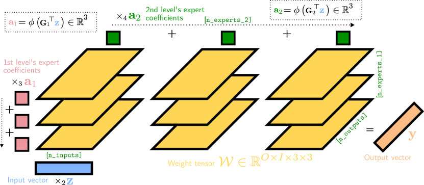
Figure 4: Illustration of a two-hierarchy MMoE layer’s (unfactorized) forward pass as a series of tensor contractions, with $3$ experts at both levels of hierarchy. The experts’ weight matrices are visualized as $2$D horizontal slices in yellow, which are (1) matrix-multiplied with the input vector, (2) summed over the first expert mode (weighted by the first expert coefficients $\mathbf{a}_{1}$ in red), and (3) summed over the second expert mode (weighted by the second expert mode’s coefficients $\mathbf{a}_{2}$ in dark green).

Here we include additional experiments with hierarchical MMoEs. Shown in Table 4(c) are the ImageNET1k test set accuracies when using MMoE layers scaling up to $4$ hierarchies, totaling $8192$ experts in the final rows. As can be seen, the increase in parameter count (as the number of experts increases) grows at a significantly slower rate than with a single hierarchy for CP and TR MMoEs in Tables 4(c) and 4(c).

As noted in the main paper, whilst TuckerMMoEs still scale drastically better than vanilla MoEs, they do not scale as well as the other two factorizations when stacking hierarchies, as can be seen by the # Params column of Table 4(c). Despite this, the number of required parameters for a single hierarchy remains low (as seen in the next column to the right).

For intuition, we further visualize the 2-hierarchy MMoE in Figure 4–note how we have an extra mode to the weight tensor, and an extra contraction over the new expert mode to combine its outputs.

Table 4: Hierarchical MMoEs: Mean test-set accuracy with a CLIP ViT-B-32 fine-tuned with hierarchical MMoE final layers on ImageNET1k. Shown are the number of parameters as the number of total experts increases to $8192$ with 4 levels of hierarchy, and the corresponding number of parameters needed for each expert total using a hierarchy $1$ MMoE, and regular MoE. Results are the average over 5 runs with different seeds. Additional expert modes for TR+TuckerMMoEs have the additional ranks set equal to the corresponding number of experts at the new mode(s) (e.g. 2 and 4).

(a) CPMMoE-r512

Hierarchy	Test acc	Weight tensor shape	Total # experts	# Params	# Params needed (w/ 1 hierarchy)	# Params needed (w/ regular MoE)
1	$73.78\pm 0.07$	$\mathcal{W}\in\mathbb{R}^{O\times I\times 128}$	128	1,069,568	1,069,568	98,432,000
2	$73.84\pm 0.11$	$\mathcal{W}\in\mathbb{R}^{O\times I\times 128\times 2}$	256	1,072,128	1,233,408	196,864,000
3	$73.80\pm 0.14$	$\mathcal{W}\in\mathbb{R}^{O\times I\times 128\times 2\times 2}$	512	1,074,688	1,561,088	393,728,000
4	$73.82\pm 0.06$	$\mathcal{W}\in\mathbb{R}^{O\times I\times 128\times 2\times 2\times 2}$	1024	1,077,248	2,216,448	787,456,000
2	$\textbf{73.89}\pm\textbf{0.10}$	$\mathcal{W}\in\mathbb{R}^{O\times I\times 128\times 4}$	512	1,074,688	1,561,088	393,728,000
3	$73.85\pm 0.08$	$\mathcal{W}\in\mathbb{R}^{O\times I\times 128\times 4\times 4}$	2048	1,079,808	3,527,168	1,574,912,000
4	$73.82\pm 0.09$	$\mathcal{W}\in\mathbb{R}^{O\times I\times 128\times 4\times 4\times 4}$	8192	1,084,928	11,391,488	6,299,648,000

(b) TRMMoE-r512

Hierarchy	Test acc	Weight tensor shape	Total # experts	# Params	# Params needed (w/ 1 hierarchy)	# Params needed (w/ regular MoE)
1	$74.66\pm 0.09$	$\mathcal{W}\in\mathbb{R}^{O\times I\times 128}$	128	3,723,264	3,723,264	98,432,000
2	$74.72\pm 0.08$	$\mathcal{W}\in\mathbb{R}^{O\times I\times 128\times 2}$	256	3,724,832	3,823,616	196,864,000
3	$74.75\pm 0.14$	$\mathcal{W}\in\mathbb{R}^{O\times I\times 128\times 2\times 2}$	512	3,726,400	4,024,320	393,728,000
4	$74.76\pm 0.11$	$\mathcal{W}\in\mathbb{R}^{O\times I\times 128\times 2\times 2\times 2}$	1024	3,727,968	8,851,456	787,456,000
2	$\textbf{74.82}\pm\textbf{0.11}$	$\mathcal{W}\in\mathbb{R}^{O\times I\times 128\times 4}$	512	3,726,400	4,024,320	393,728,000
3	$74.67\pm 0.12$	$\mathcal{W}\in\mathbb{R}^{O\times I\times 128\times 4\times 4}$	2048	3,729,536	5,228,544	1,574,912,000
4	$74.73\pm 0.11$	$\mathcal{W}\in\mathbb{R}^{O\times I\times 128\times 4\times 4\times 4}$	8192	3,732,672	10,045,440	6,299,648,000

(c) TuckerMMoE-r64

Hierarchy	Test acc	Weight tensor shape	Total # experts	# Params	# Params needed (w/ 1 hierarchy)	# Params needed (w/ regular MoE)
1	$71.90\pm 0.05$	$\mathcal{W}\in\mathbb{R}^{O\times I\times 128}$	128	481,856	481,856	98,432,000
2	$72.18\pm 0.09$	$\mathcal{W}\in\mathbb{R}^{O\times I\times 128\times 2}$	256	745,540	588,352	196,864,000
3	$72.39\pm 0.13$	$\mathcal{W}\in\mathbb{R}^{O\times I\times 128\times 2\times 2}$	512	1,271,368	801,344	393,728,000
4	$72.45\pm 0.07$	$\mathcal{W}\in\mathbb{R}^{O\times I\times 128\times 2\times 2\times 2}$	1024	2,321,484	1,227,328	787,456,000
2	$72.40\pm 0.09$	$\mathcal{W}\in\mathbb{R}^{O\times I\times 128\times 4}$	512	1,271,376	801,344	393,728,000
3	$\textbf{72.53}\pm\textbf{0.07}$	$\mathcal{W}\in\mathbb{R}^{O\times I\times 128\times 4\times 4}$	2048	4,420,192	2,079,296	1,574,912,000
4	$72.15\pm 0.10$	$\mathcal{W}\in\mathbb{R}^{O\times I\times 128\times 4\times 4\times 4}$	8192	17,006,192	7,191,104	6,299,648,000

Appendix D Expert modularity: additional results

Qualitative visualization

Additional results to further substantiate the claims in the main paper about expert class-modularity are presented here. Firstly in Figure 7 are many more random images (of those with expert coefficient $\geq 0.5$) of the first few experts as they are ordered numerically. Furthermore, when we use an even larger number of experts (i.e. $2048$) we observe a select few experts developing what appear to be very fine-grained specialisms, as shown in Figure 8. For example, images with large coefficients for #$203$ are often animals on top of laptops, whilst images with high coefficients for #$1203$ are animals eating corn.

Counterfactual intervention barplots

Next, we show barplots of the class labels whose test set accuracies are most changed under the counterfactual question in the main paper: “had (expert $n$) not contributed its weight, how would the class predictions have changed?”. These are shown in Figure 5 and Figure 6 when using a CPMMoE as a final and penultimate layer respectively. As can be seen, we often observe that a higher number of experts (the final rows in brown color) lead to experts that, upon ablation, cause the model to lose almost all its accuracy for fewer classes. Experts here are chosen in numerical order and only those yielding $\geq 0.5$ total accuracy change to any class upon counterfactual ablation.

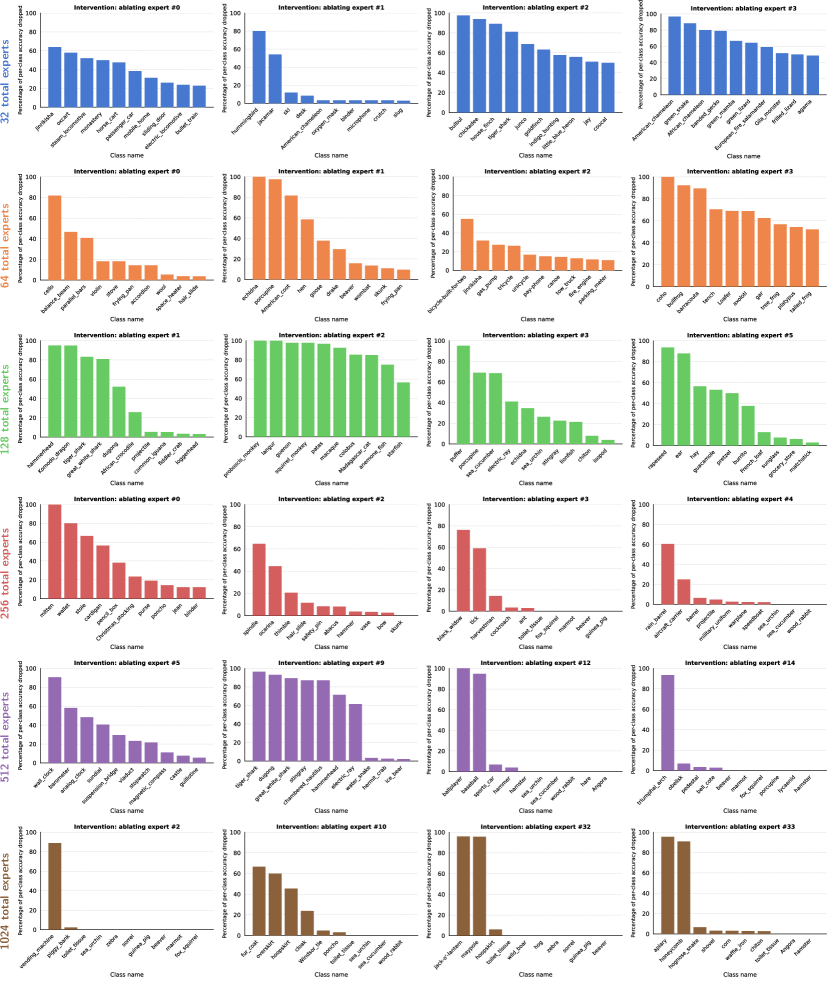
Figure 5: Penultimate layer CPMMoE: Percentage of per-class test set accuracy lost when intervening and ablating particular experts (along the columns). In general, the more total experts (rows), the more class-level monosemantic the experts are as indicated by the mass centred on fewer classes, and with higher magnitude. Shown are the first $4$ experts in each model (row) to change $\geq 0.5$ of any class’ accuracy when counterfactually ablated.

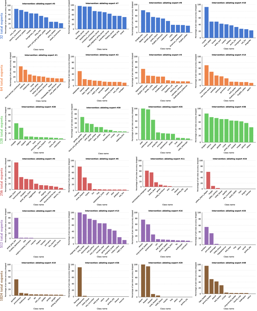
Figure 6: Final layer CPMMoE: Percentage of per-class test set accuracy lost when intervening and ablating particular experts (along the columns). In general, the more total experts (rows), the more class-level monosemantic the experts are as indicated by the mass centred on fewer classes, and with higher magnitude. Shown are the first $4$ experts in each model (row) to change $\geq 0.5$ of any class’ accuracy when counterfactually ablated.

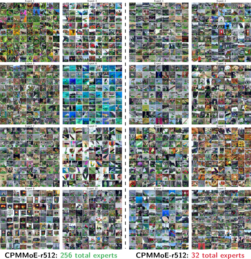
Figure 7: $256$ vs $32$ total experts: Randomly selected training set images with expert coefficient $\geq 0.5$ for the first $10$ numerical experts (of those processing any images with coefficient $\geq 0.5$). Results are with CP-r512 MMoE layers with 256 (left) and 32 (right) total experts respectively. We highlight the apparent specialism of the experts when a higher total number is used. (Please zoom for detail)

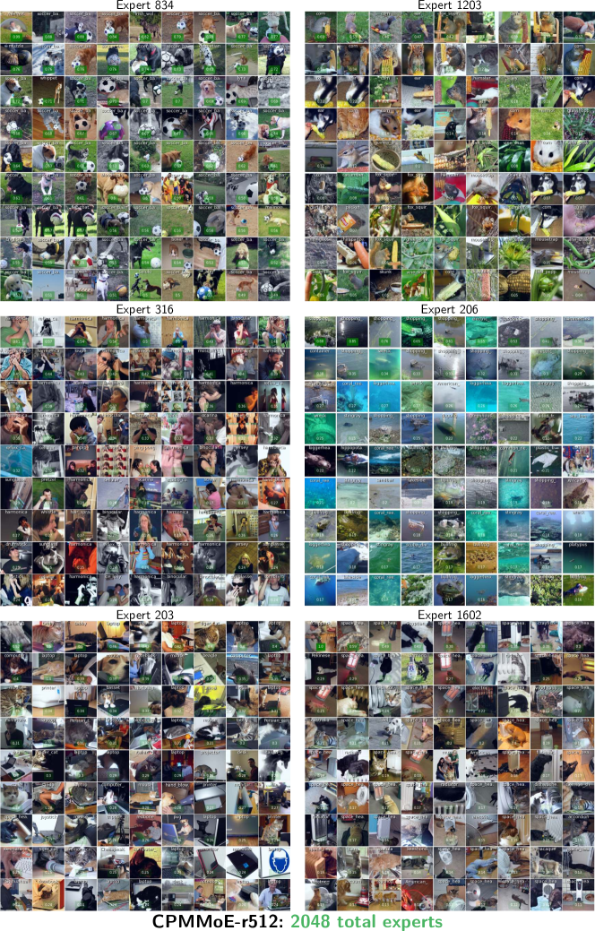
Figure 8: Fine-grained expert specialisms: Manually selected experts (and images ranked by highest expert coefficients) learnt to process very fine-grained categories (e.g. animals with footballs, trolleys in water, etc.). Model trained on ImageNET1k with a high number of $2048$ experts and a CP-r512 MMoE layer. (Please zoom for detail)

Appendix E Ablation studies

Entax vs softmax

We find the use of the entmax activation function (Peters et al., 2019; Correia et al., 2019) to produce more monosemantic experts, as quantified by the measure of polysemanticity used in the main paper. We show in Figure 9 the mean expert polysemanticity (of those experts that affect the class accuracy upon ablation) for CPMMoE-r512 final layer models fine-tuned with an various numbers of experts. As can be seen, the entmax function consistently produces more monosemantic experts for larger total expert counts. We attribute this to the sparsity in entmax’s post-activation distribution (whereas the softmax function can just as readily output a uniform distribution over all expert coefficients).

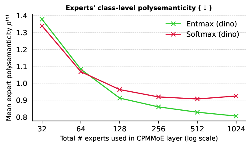
(a) DINO backbone

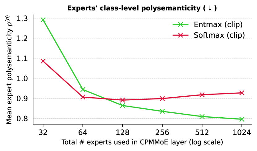
(b) CLIP backbone

Figure 9: Softmax vs Entmax ablation CPMMoE-r512 final layers trained on ImageNET, and the resulting class-level polysemanticity. For large values of experts, the entmax activation produces more specialized experts.

Fast vs naive forward pass speedups

We include here a study of model choice on the number of FLOPs relative to Soft MoEs. In Figure 10 we show a plot of the parameter counts. Here we observe the properties of CPMMoEs detailed in the main paper. In particular, we see (in the orange plot) the number of parameters (and consequently; FLOPs) to be relatively small for low numbers of experts, but overtake the other MMoE models as $N$ grows very large.

Fast computation speedups

We next plot in Figure 11 the actual number of FLOPs when executing PyTorch MMoE layers using the naive forward pass relative to the cost when using the factorized model forms–the fast computation is many orders of magnitude less expensive.

E.1 Expert load

Here, we plot the expert load in Figure 12 to give a visual indication of how many images are processed by each expert with $a_{e}\geq 0.5$ for CPMMoE final layers fine-tuned on ImageNET1k with a CLIP backbone. Whilst clearly not all experts have images with coefficient of at least $0.5$, we see a relatively uniform spread over all experts. Furthermore, we note the cost from ‘dead’ experts is not particularly troublesome in an MMoE given its factorized form–speaking informally, we would rather have too many experts than too few, so long as there exist select individual experts conducting the subcomputations of interest.

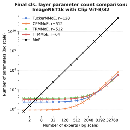
Figure 10: Theoretical parameter count vs number of linear experts used (log-log scale); note the CPMMoE’s increase in cost trend for very large $N$, relative to other variants.

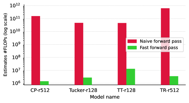
Figure 11: Fast vs naive forward pass FLOP comparison Number of FLOPs in each layer’s PyTorch forward pass (with $512$ experts and a $768$-dimensional input and output vector). Naive implementation in Section 3.1 is compared to equivalent einsum implementations of Equations 2, 4 and 3.

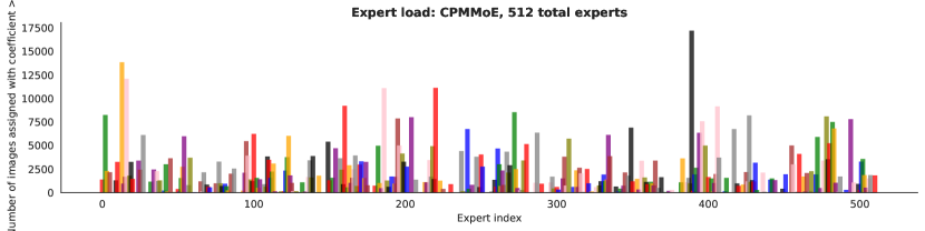
(a) $512$ total experts

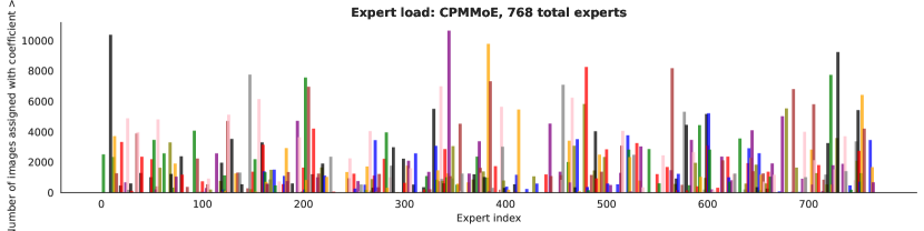
(b) $768$ total experts

Figure 12: Expert load: Number of training set images with expert coefficient $a_{n}\geq 0.5$ for CPMMoE models fine-tuned on ImageNET1k. Bars are drawn with 3x width and colored sequentially in a repeating order of distinct colors to help visually distinguish between neighbors.

Appendix F Additional performance results

Here, we include extensive results fine-tuning MMoE final layer foundational models on a range of datasets, iterating from $2$ total experts to $16000$, comparing at the same time across MMoE variants as the expert count increases and their parameter-matched linear layer counterparts. We first plot all the results visually in Figure 13 for CLIP models, and display in table form in Table 6 a more readable slice of the results for $N=128$ experts. The same results are shown in Figure 14 and Table 7 respectively for a DINO backbone.

MLP mixer

Whilst the primary goal of MMoE layers is to aid interpretability through scalable expert specialization, it’s important that the layers also retain competitive performance. Here we show tentative initial evidence that MMoE layers can be used to replace MLP layers more generally in small-scale models trained from scratch, and that performance is indeed competitive with existing MLP layer counterparts. Concretely, we train S/16 MLP mixer variants from scratch, following the model specification in Tolstikhin et al. (2021), building off the open-source model code in https://github.com/lucidrains/mlp-mixer-pytorch. We replace all MLPs in the mixer layers with CPMMoE layers, each with $128$ experts. The CP ranks are set to be $3.25$ times the dimension of the input channels (this value is chosen to approximately match the total number of parameters in the MLP-Mixer). This results in $18$M trainable parameters for the original MLP-Mixer model and $19$M for the CPMMoE.

We train all models from scratch for $300$ epochs using a cosine learning rate scheduler with $10,000$ warmup steps. We use the AdamW optimizer with learning rate $0.001$, and a regularization strength of $0.1$. No regularization is applied to either the bias or layer norm parameters. For MMoEs, we also use no regularization for the factors for the expert and output modes of the tensors. We use 2 layers of RandAugment with magnitude $10$, dropout rate of $0.1$, Mixup with $\alpha=0.5$, inception cropping, random horizontal flipping, and gradient clipping. We find stochastic depth to harm the performance of all S/16 MLP/MMoE models, so we do not use it. We use the same batch size of $4096$ as Tolstikhin et al. (2021), made possible through mixed-precision training across 4 $80$GB A100 GPUs using the Accelerate library (Gugger et al., 2022).

The preliminary results are included in Table 5, where we can see that the CPMMoE-mixer competes favorably with our results from training the original MLP-mixer S/16 architecture. As also noted in the paper (Tolstikhin et al., 2021), we find both MLP and MMoE mixers very prone to overfitting, producing poor results on some of the smaller-scale datasets however (e.g. Caltech256, TinyImageNET).

Table 5: MLP-mixer S/16 test set (validation set for ImageNET1k) accuracy at $300$ epochs with the usual 2-layer MLP vs parameter-matched CPMMoE variants with $128$ experts.

	ImageNET1k	CIFAR100	Food101	Caltech101	Caltech256	TinyImageNET
MLP (2-layer; original)	50.75	65.54	66.33	53.57	25.19	47.46
CPMMoE (ours)	59.85	65.95	68.17	50.92	26.04	48.45

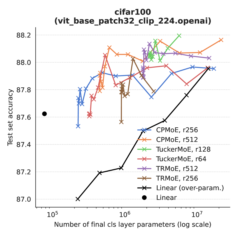
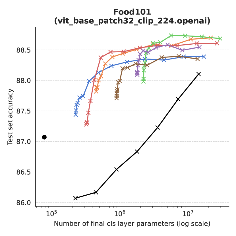
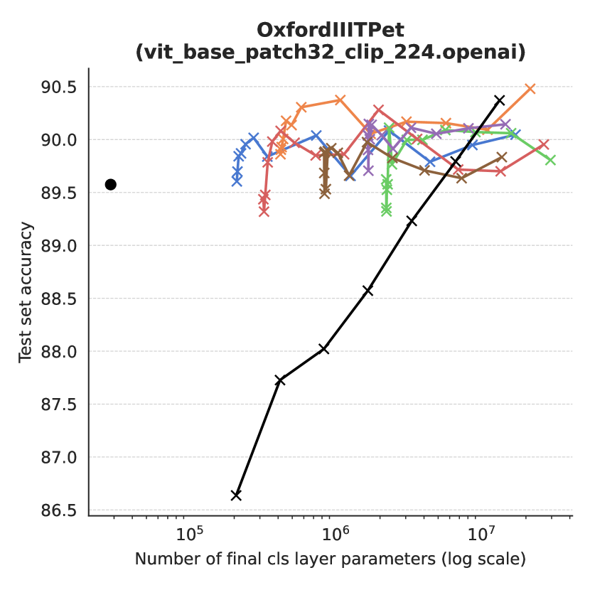
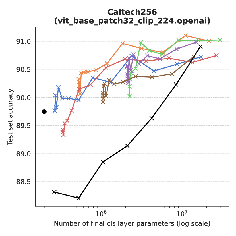
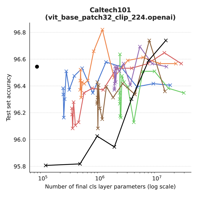
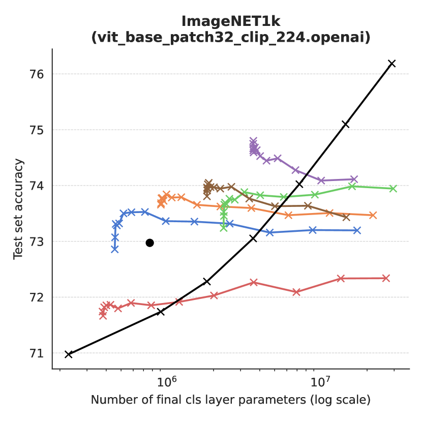
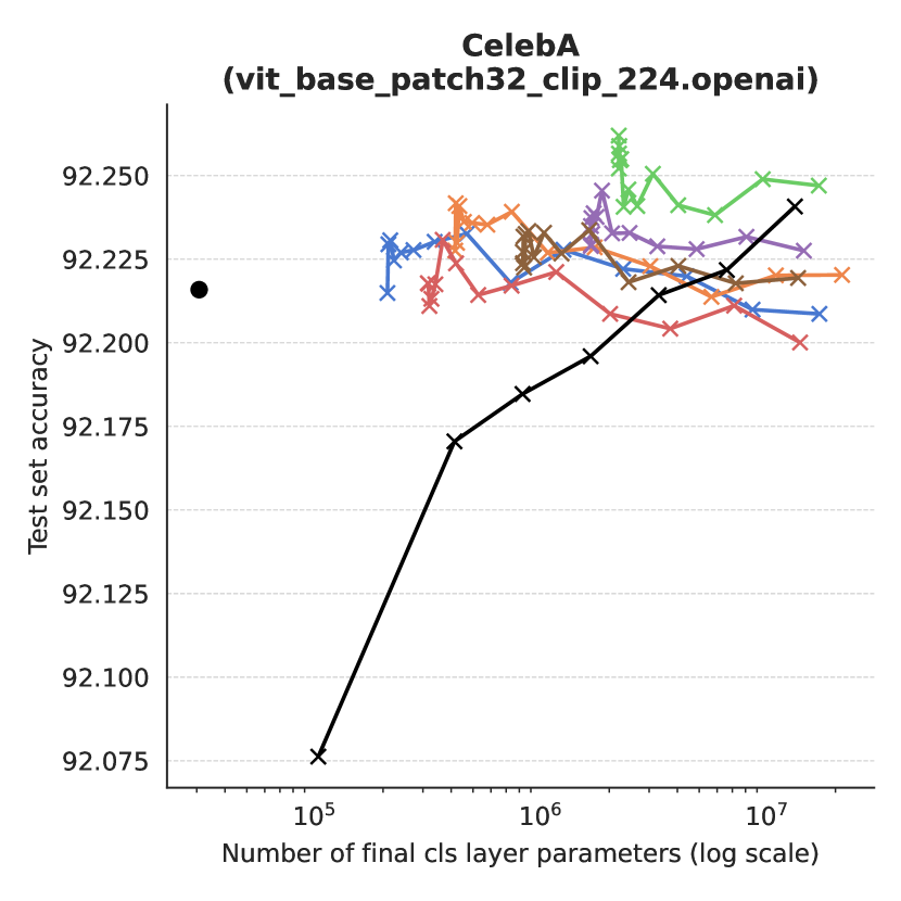
Figure 13: Parameter-matched fine-tuning with CLIP ViT-B-32 as the total # experts increases. All results are averaged over $10$ random seeds ($5$ for ImageNET1k)

Table 6: Test set accuracy fine-tuning a CLIP vit_base_patch32 model. Average results are reported over $10$ random seeds ($5$ for ImageNET1k). Comparisons are made to regular linear layers and CPMMoE-r512 parameter-matched linear layers.

	Test set accuracy								Number of layer parameters
	CIFAR100	Caltech256	Caltech101	Food101	OxfordIIITPet	CelebA	ImageNET1k		CIFAR100	Caltech256	Caltech101	Food101	OxfordIIITPet	CelebA	ImageNET1k
MLP	$87.62\pm 0.16$	$89.75\pm 0.5$	$\textbf{96.54}\pm\textbf{0.59}$	$87.07\pm 0.06$	$89.57\pm 0.49$	$92.22\pm 0.02$	$72.97\pm 0.07$		76900	197633	78438	77669	28453	30760	769000
HighRankMLP	$87.23\pm 0.25$	$88.85\pm 0.57$	$96.03\pm 0.67$	$86.54\pm 0.12$	$88.02\pm 0.45$	$92.18\pm 0.01$	$72.28\pm 0.14$		888932	1049857	890982	889957	824357	827432	1811432
CPMMoE-r256	$87.88\pm 0.18$	$89.98\pm 0.66$	$96.47\pm 0.59$	$87.99\pm 0.07$	$89.84\pm 0.33$	$92.23\pm 0.02$	$73.52\pm 0.10$		353536	393728	354048	353792	337408	338176	583936
CPMMoE-r512	$\textbf{88.11}\pm\textbf{0.15}$	$90.46\pm 0.57$	$96.44\pm 0.77$	$88.27\pm 0.10$	$\textbf{90.31}\pm\textbf{0.52}$	$\textbf{92.24}\pm\textbf{0.02}$	$73.78\pm 0.07$		608768	689152	609792	609280	576512	578048	1069568
TuckerMMoE-r128	$88.04\pm 0.13$	$90.46\pm 0.61$	$96.47\pm 0.31$	$\textbf{88.45}\pm\textbf{0.16}$	$89.77\pm 0.22$	$\textbf{92.24}\pm\textbf{0.01}$	$73.76\pm 0.06$		2421376	2441472	2421632	2421504	2413312	2315392	2536576
TuckerMMoE-r64	$87.82\pm 0.18$	$90.14\pm 0.37$	$96.35\pm 0.68$	$88.38\pm 0.14$	$89.97\pm 0.42$	$92.22\pm 0.02$	$71.90\pm 0.05$		424256	532608	522688	522624	518528	420416	580160
TRMMoE-r512	$88.07\pm 0.14$	$\textbf{90.70}\pm\textbf{0.50}$	$96.43\pm 0.66$	$88.33\pm 0.10$	$90.14\pm 0.41$	$\textbf{92.24}\pm\textbf{0.01}$	$\textbf{74.68}\pm\textbf{0.03}$		1880064	2201600	1884160	1882112	1751040	1757184	3723264
TRMMoE-r256	$87.75\pm 0.17$	$90.03\pm 0.51$	$96.23\pm 0.65$	$87.99\pm 0.11$	$89.92\pm 0.54$	$92.23\pm 0.01$	$73.97\pm 0.09$		990208	1150976	992256	991232	925696	928768	1911808

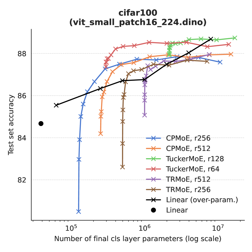
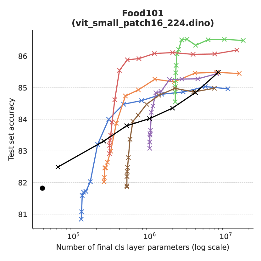
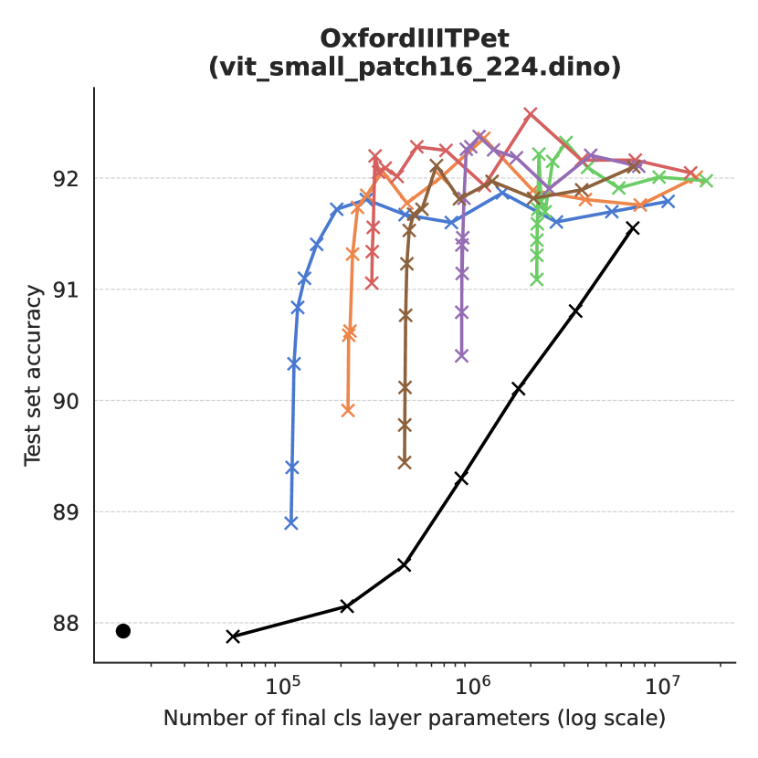
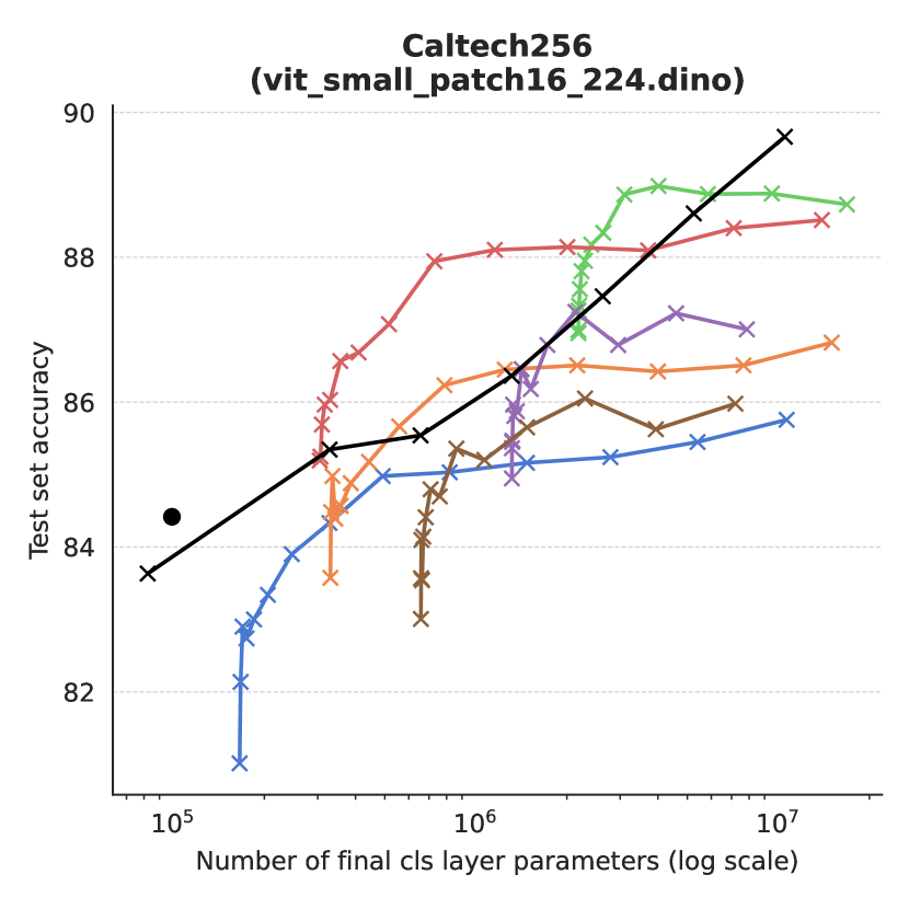
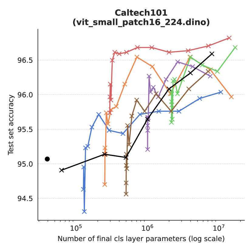
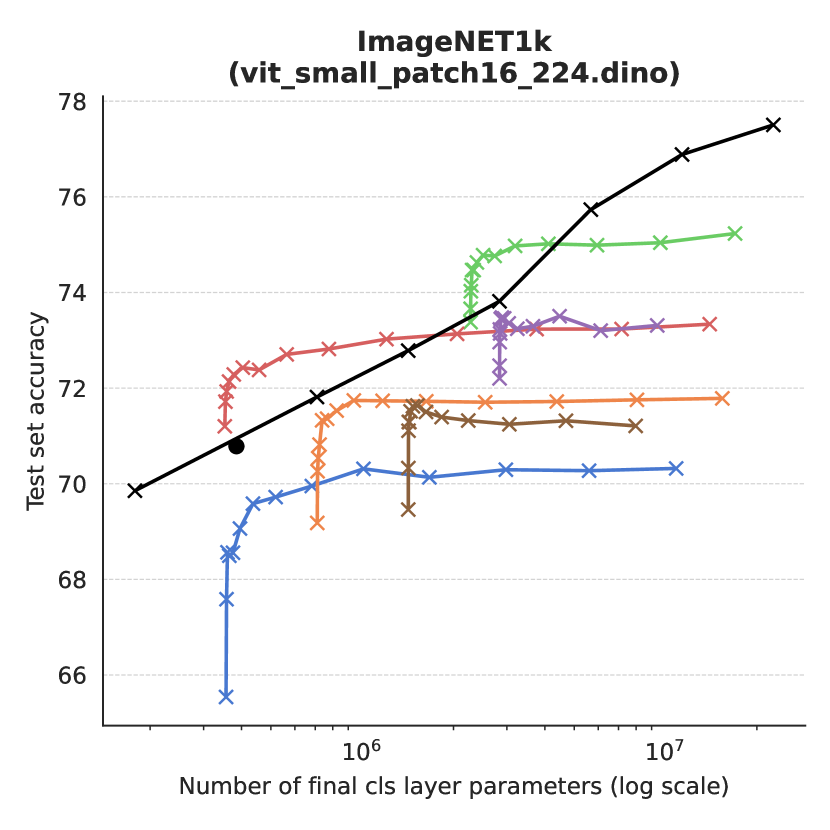
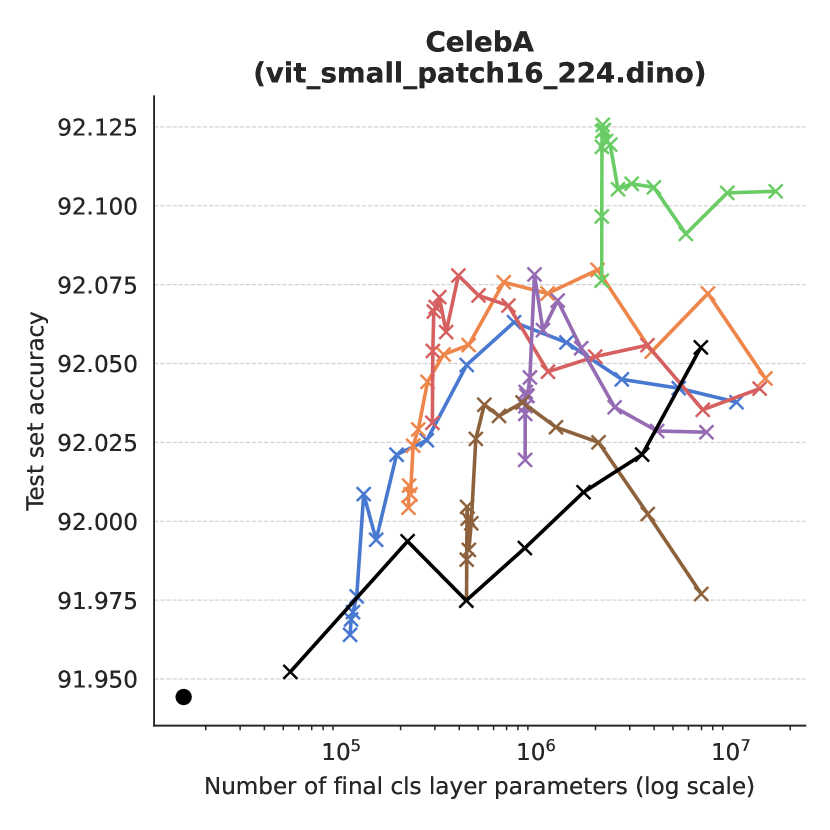
Figure 14: Parameter-matched fine-tuning with dino-small-patch16 as the total # experts increases. All results are averaged over 5 random seeds.

Table 7: Test set accuracy fine-tuning a DINO vit_small_patch16_224 model. Average results are reported over $5$ random seeds. Comparisons are made to regular linear layers and CPMMoE-r512 parameter-matched linear layers.

	Test set accuracy								Number of layer parameters
	CIFAR100	Caltech256	Caltech101	Food101	OxfordIIITPet	CelebA	ImageNET1k		CIFAR100	Caltech256	Caltech101	Food101	OxfordIIITPet	CelebA	ImageNET1k
MLP	$84.67\pm 0.34$	$84.42\pm 0.46$	$95.07\pm 0.54$	$81.82\pm 0.28$	$87.93\pm 0.68$	$91.94\pm 0.01$	$70.78\pm 0.73$		38500	98945	39270	38885	14245	15400	385000
HighRankMLP	$87.19\pm 0.17$	$\textbf{88.21}\pm\textbf{0.62}$	$95.82\pm 0.65$	$\textbf{86.17}\pm\textbf{0.12}$	$87.73\pm 0.61$	$\textbf{92.17}\pm\textbf{0.01}$	$71.74\pm 0.04$		444516	525057	445542	445029	412197	413736	906216
CPMMoE-r256	$86.66\pm 0.13$	$83.90\pm 0.41$	$95.71\pm 0.94$	$83.21\pm 0.18$	$91.72\pm 0.26$	$92.02\pm 0.01$	$69.58\pm 0.42$		206080	246272	206592	206336	189952	190720	436480
CPMMoE-r512	$87.14\pm 0.20$	$85.17\pm 0.52$	$95.83\pm 0.76$	$83.87\pm 0.21$	$92.06\pm 0.35$	$92.05\pm 0.01$	$71.53\pm 0.15$		363008	443392	364032	363520	330752	332288	823808
TuckerMMoE-r128	$\textbf{88.44}\pm\textbf{0.21}$	$87.95\pm 0.43$	$96.20\pm 0.56$	$86.07\pm 0.10$	$91.79\pm 0.14$	$92.12\pm 0.01$	$\textbf{74.63}\pm\textbf{0.15}$		2273920	2294016	2274176	2274048	2265856	2266240	2389120
TuckerMMoE-r64	$88.22\pm 0.22$	$86.68\pm 0.57$	$\textbf{96.59}\pm\textbf{0.65}$	$85.55\pm 0.06$	$92.01\pm 0.26$	$92.08\pm 0.02$	$72.38\pm 0.08$		399680	409728	399808	399744	395648	395840	457280
TRMMoE-r512	$86.94\pm 0.20$	$85.87\pm 0.64$	$96.27\pm 0.82$	$84.22\pm 0.12$	$\textbf{92.26}\pm\textbf{0.20}$	$92.05\pm 0.01$	$73.48\pm 0.15$		1044480	1366016	1048576	1046528	915456	921600	2887680
TRMMoE-r256	$86.65\pm 0.27$	$84.80\pm 0.66$	$95.28\pm 0.48$	$83.37\pm 0.07$	$91.68\pm 0.26$	$92.03\pm 0.02$	$71.62\pm 0.05$		547840	708608	549888	548864	483328	486400	1469440

Appendix G Fairness baselines & metric details

Here we present more details about the fairness comparisons and metrics used in the main paper.

Metrics

• Equality of opportunity requires the true positive rates for the sensitive attribute subpopulations to be equal, defined in Hardt et al. (2016) as $P(\hat{Y}=1|A=0,Y=1)=P(\hat{Y}=1|A=1,Y=1)$ for sensitive attribute $A$, target attribute $Y$, and predictor $\hat{Y}$. In the first of our CelebA experiments we measure the absolute difference of the true positive rates between the ‘blond female’ and ‘blond male’ subpopulations for the ‘blond hair’ target attribute. For the second we measure the difference between that of the ‘old female’ and ‘old male’ subpopulations, taking the ‘old’ label as the true target attribute.

• Standard deviation bias computes the standard deviation of the accuracy for the different subpopulations (Wang & Deng, 2020). Intuitively, a small STD bias indicates similar performance across groups.

• Max-Min Fairness quantifies the worst-case performance for the different demographic subpopulations (Lahoti et al., 2020), with $\max\min_{y\in\mathcal{Y},a\in\mathcal{A}}P(\hat{Y}=y|A=a,Y=y)$. We compute this as the minimum of the test-set accuracy for the $4$ subpopulations in each experiment.

Baselines

• Oversample we oversample the low-support subpopulation to balance the number of input images that have the sensitive attribute for the value of the target attribute wherein bias occurs. For example, we oversample the ‘blond males’ to match the number of ‘blond females’ for the first experiment, and oversample the number of ‘old females’ to match the number of ‘old males’ for the second.

• Blind thresholding is implemented by unconditionally increasing/decreasing the logits in the target direction for all outputs. Concretely, the results in the main paper are achieved by setting $\lambda:=2.5$ and $\bar{\mathbf{a}}$ to a vector of ones in Equation 6 for all experiments. We find this value of $\lambda$ to give us the best results for the attribute-blind re-writing (Hardt et al., 2016).

• Adversarial debiasing we observe in Table 2 the same poor performance for the adversarial debiasing technique as is reported in Wang et al. (2020). We hypothesize that the same issues face the technique in our experimental setup. In particular, even in the absence of discriminative information for the ‘gender’ label in the final representation, information about correlated attributes (e.g. wearing makeup) are likely still present. This makes it fundamentally challenging to apply fairness-through-unawareness techniques in the CelebA multi-class setting.

Appendix H Model re-writing: additional results

The full per-subpopulation test set accuracies are shown in Figure 16 for the two experiments in the main paper. The first rows show the accuracies before layer re-write, the second rows after re-write, and the third rows the absolute difference between the two. As can be seen in the ‘before-after difference’ final rows of Figure 16, the proposed expert-conditional re-write provides much more precision in changing only the computation for the target populations.

Furthermore, we include the ‘model re-writing’ score results for all MMoE variants and its comparison to an attribute/expert-blind variant in Figure 15. Clearly–across all MMoE configurations–the expert conditional re-writing allows more precise correction of bias in CelebA.

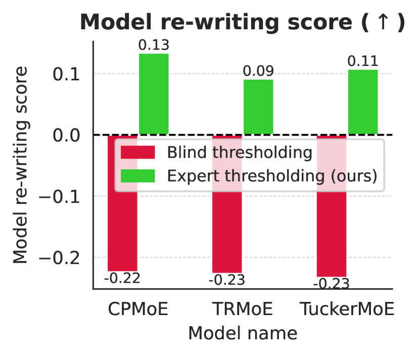
(a) ‘Old female’ target subpop. for age prediction.

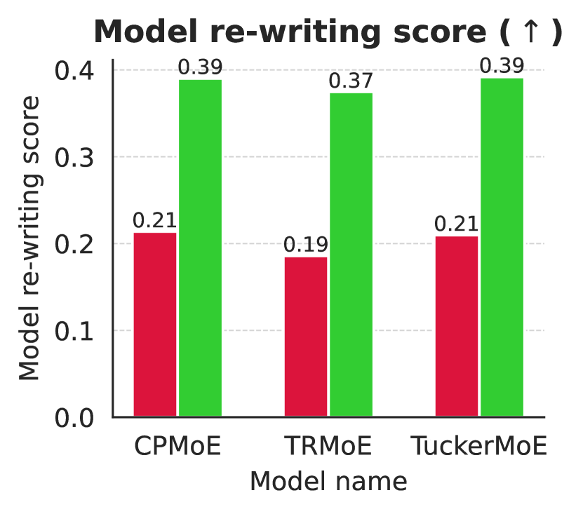
(b) ‘Blond male’ target subpop. for blond hair prediction.

Figure 15: ‘Model re-writing score’ quantifying fairness interventions for two demographic biases in CelebA for all MMoE variants. $128$ experts are used throughout.

Table 8: Additional comparisons of the MMoE layer expert-conditional layer re-writing to the static unconditional fairness thresholding (Hardt et al., 2016), for many more MMoE variants.

(c) Bias towards ‘Old females’ for ‘Age’ prediction head

	Model re-write score ($\uparrow$)	Target subpop. acc. ($\uparrow$)	Equality of opp. ($\downarrow$)	Std deviation bias ($\downarrow$)	Subpop. Max-Min ($\uparrow$)	Test acc. ($\uparrow$)	# layer params ($\downarrow$)
CPMMoE-r512-e128 + blind thresholding (Hardt et al., 2016)	-0.224	0.843	0.082	0.084	0.700	83.369	578048
CPMMoE-r512-e128 + expert thresholding (ours)	0.134	0.866	0.097	0.066	0.756	84.650	578048
TRMMoE-r512-e128 + blind thresholding (Hardt et al., 2016)	-0.227	0.847	0.079	0.084	0.700	83.296	1757184
TRMMoE-r512-e128 + expert thresholding (ours)	0.092	0.917	0.145	0.084	0.733	81.110	1757184
TuckerMMoE-r64-e128 + blind thresholding (Hardt et al., 2016)	-0.233	0.838	0.088	0.084	0.699	83.406	518720
TuckerMMoE-r64-e128 + expert thresholding (ours)	0.108	0.884	0.110	0.064	0.764	83.430	518720

(d) Bias towards ‘Blond males’ for ‘Blond Hair’ prediction head

	Model re-write score ($\uparrow$)	Target subpop. acc. ($\uparrow$)	Equality of opp. ($\downarrow$)	Std deviation bias ($\downarrow$)	Subpop. Max-Min ($\uparrow$)	Test acc. ($\uparrow$)	# layer params ($\downarrow$)
CPMMoE-r512-e128 + blind thresholding (Hardt et al., 2016)	0.214	0.843	0.139	0.063	0.841	92.447	578048
CPMMoE-r512-e128 + expert thresholding (ours)	0.390	0.847	0.051	0.048	0.846	94.895	578048
TRMMoE-r512-e128 + blind thresholding (Hardt et al., 2016)	0.186	0.837	0.145	0.064	0.837	92.565	1757184
TRMMoE-r512-e128 + expert thresholding (ours)	0.375	0.869	0.035	0.038	0.866	94.582	1757184
TuckerMMoE-r64-e128 + blind thresholding (Hardt et al., 2016)	0.210	0.830	0.152	0.067	0.829	92.541	518720
TuckerMMoE-r64-e128 + expert thresholding (ours)	0.392	0.876	0.049	0.036	0.866	94.072	518720

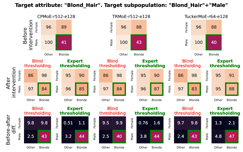
(a) ‘Young blond’ intervention for Blond hair attribute prediction head

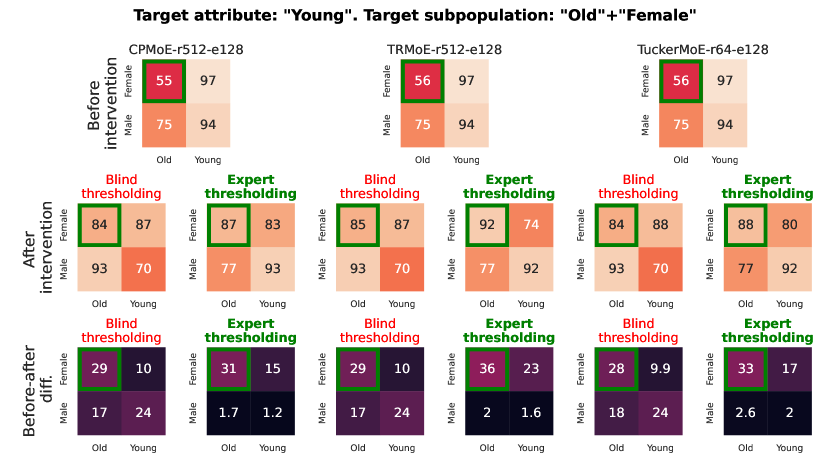
(b) ‘Old female’ intervention for age attribute prediction head

Figure 16: CelebA Subpopulation accuracies before (first rows) and after intervention (second rows), followed by their absolute difference (third rows). Green rectangles denote the target subpopulation for each experiment (subfigure).

References

- Alvi et al. (2018) Alvi, M., Zisserman, A., and Nellåker, C. Turning a blind eye: Explicit removal of biases and variation from deep neural network embeddings. In Proceedings of the European Conference on Computer Vision (ECCV) Workshops, 2018.
- Babiloni et al. (2020) Babiloni, F., Marras, I., Slabaugh, G., and Zafeiriou, S. Tesa: Tensor element self-attention via matricization. In IEEE Conf. Comput. Vis. Pattern Recog. (CVPR), pp. 13945–13954, 2020.
- Babiloni et al. (2021) Babiloni, F., Marras, I., Kokkinos, F., Deng, J., Chrysos, G., and Zafeiriou, S. Poly-nl: Linear complexity non-local layers with 3rd order polynomials. In Int. Conf. Comput. Vis. (ICCV), pp. 10518–10528, 2021.
- Babiloni et al. (2023) Babiloni, F., Tanay, T., Deng, J., Maggioni, M., and Zafeiriou, S. Factorized dynamic fully-connected layers for neural networks. In Int. Conf. Comput. Vis. Worksh. (ICCVW), pp. 1374–1383, October 2023.
- Bengio et al. (2015) Bengio, E., Bacon, P.-L., Pineau, J., and Precup, D. Conditional computation in neural networks for faster models. In Int. Conf. Mach. Learn. Worksh. (ICMLW), 2015.
- Bolukbasi et al. (2021) Bolukbasi, T., Pearce, A., Yuan, A., Coenen, A., Reif, E., Viégas, F., and Wattenberg, M. An interpretability illusion for bert. arXiv preprint arXiv:2104.07143, 2021.
- Bulat et al. (2020) Bulat, A., Kossaifi, J., Tzimiropoulos, G., and Pantic, M. Incremental multi-domain learning with network latent tensor factorization. In Conf. on Artifi. Intel. (AAAI), volume 34, pp. 10470–10477, 2020.
- Buolamwini & Gebru (2018) Buolamwini, J. and Gebru, T. Gender shades: Intersectional accuracy disparities in commercial gender classification. In Conference on fairness, accountability and transparency, pp. 77–91. PMLR, 2018.
- Caron et al. (2021) Caron, M., Touvron, H., Misra, I., Jégou, H., Mairal, J., Bojanowski, P., and Joulin, A. Emerging properties in self-supervised vision transformers. In Int. Conf. Comput. Vis. (ICCV), 2021.
- Carroll & Chang (1970) Carroll, J. D. and Chang, J. J. Analysis of individual differences in multidimensional scaling via an n-way generalization of “eckart-young” decomposition. Psychometrika, 35:283–319, 1970.
- Casper (2023) Casper, S. Broad critiques of interpretability research. 2023. URL https://www.alignmentforum.org/s/a6ne2ve5uturEEQK7/p/gwG9uqw255gafjYN4.
- Chen et al. (2020) Chen, Y., Dai, X., Liu, M., Chen, D., Yuan, L., and Liu, Z. Dynamic convolution: Attention over convolution kernels. In IEEE Conf. Comput. Vis. Pattern Recog. (CVPR), pp. 11030–11039, 2020.
- Cheng et al. (2024) Cheng, Y., Chrysos, G. G., Georgopoulos, M., and Cevher, V. Multilinear operator networks, 2024.
- Cherepanova et al. (2021) Cherepanova, V., Nanda, V., Goldblum, M., Dickerson, J. P., and Goldstein, T. Technical challenges for training fair neural networks. arXiv preprint arXiv:2102.06764, 2021.
- Chrysos et al. (2020) Chrysos, G. G., Moschoglou, S., Bouritsas, G., Panagakis, Y., Deng, J., and Zafeiriou, S. P-nets: Deep polynomial neural networks. In IEEE Conf. Comput. Vis. Pattern Recog. (CVPR), pp. 7325–7335, 2020.
- Chrysos et al. (2021) Chrysos, G. G., Moschoglou, S., Bouritsas, G., Deng, J., Panagakis, Y., and Zafeiriou, S. P. Deep polynomial neural networks. IEEE Trans. Pattern Anal. Mach. Intell. (TPAMI), pp. 1–1, 2021. ISSN 1939-3539.
- Correia et al. (2019) Correia, G. M., Niculae, V., and Martins, A. F. T. Adaptively sparse transformers. In Inui, K., Jiang, J., Ng, V., and Wan, X. (eds.), Proceedings of the 2019 Conference on Empirical Methods in Natural Language Processing and the 9th International Joint Conference on Natural Language Processing (EMNLP-IJCNLP), pp. 2174–2184, Hong Kong, China, November 2019. Association for Computational Linguistics. doi: 10.18653/v1/D19-1223.
- Davis & Arel (2013) Davis, A. and Arel, I. Low-rank approximations for conditional feedforward computation in deep neural networks. arXiv preprint arXiv:1312.4461, 2013.
- De Lathauwer et al. (2000) De Lathauwer, L., De Moor, B., and Vandewalle, J. On the best rank-1 and rank-(r1 ,r2 ,. . .,rn) approximation of higher-order tensors. SIAM Journal on Matrix Analysis and Applications, 21(4):1324–1342, 2000. doi: 10.1137/S0895479898346995.
- Deng et al. (2009) Deng, J., Dong, W., Socher, R., Li, L.-J., Li, K., and Fei-Fei, L. Imagenet: A large-scale hierarchical image database. In IEEE Conf. Comput. Vis. Pattern Recog. (CVPR), pp. 248–255, 2009.
- Du et al. (2022) Du, N., Huang, Y., Dai, A. M., Tong, S., Lepikhin, D., Xu, Y., Krikun, M., Zhou, Y., Yu, A. W., Firat, O., et al. Glam: Efficient scaling of language models with mixture-of-experts. In Int. Conf. Mach. Learn. (ICML), pp. 5547–5569. PMLR, 2022.
- Eigen et al. (2013) Eigen, D., Ranzato, M., and Sutskever, I. Learning factored representations in a deep mixture of experts. In Int. Conf. Mach. Learn. Worksh. (ICMLW), volume abs/1312.4314, 2013.
- Elazar et al. (2021) Elazar, Y., Ravfogel, S., Jacovi, A., and Goldberg, Y. Amnesic probing: Behavioral explanation with amnesic counterfactuals. Transactions of the Association for Computational Linguistics, 9:160–175, 2021.
- Elhage et al. (2022) Elhage, N., Hume, T., Olsson, C., Schiefer, N., Henighan, T., Kravec, S., Hatfield-Dodds, Z., Lasenby, R., Drain, D., Chen, C., et al. Toy models of superposition. arXiv preprint arXiv:2209.10652, 2022.
- Fedus et al. (2022) Fedus, W., Zoph, B., and Shazeer, N. Switch transformers: Scaling to trillion parameter models with simple and efficient sparsity. The Journal of Machine Learning Research, 23(1):5232–5270, 2022.
- Gale et al. (2023) Gale, T., Narayanan, D., Young, C., and Zaharia, M. Megablocks: Efficient sparse training with mixture-of-experts. Proceedings of Machine Learning and Systems, 5, 2023.
- Gao et al. (2022) Gao, Z.-F., Liu, P., Zhao, W. X., Lu, Z.-Y., and Wen, J.-R. Parameter-efficient mixture-of-experts architecture for pre-trained language models. In Proceedings of the 29th International Conference on Computational Linguistics, Gyeongju, Republic of Korea, October 2022. International Committee on Computational Linguistics.
- Garipov et al. (2016) Garipov, T., Podoprikhin, D., Novikov, A., and Vetrov, D. Ultimate tensorization: compressing convolutional and fc layers alike. arXiv preprint arXiv:1611.03214, 2016.
- Gebru et al. (2021) Gebru, T., Morgenstern, J., Vecchione, B., Vaughan, J. W., Wallach, H., Iii, H. D., and Crawford, K. Datasheets for datasets. Communications of the ACM, 64(12):86–92, 2021.
- Georgopoulos et al. (2020) Georgopoulos, M., Chrysos, G., Pantic, M., and Panagakis, Y. Multilinear latent conditioning for generating unseen attribute combinations. In Int. Conf. Mach. Learn. (ICML), 2020.
- Georgopoulos et al. (2021) Georgopoulos, M., Oldfield, J., Nicolaou, M. A., Panagakis, Y., and Pantic, M. Mitigating demographic bias in facial datasets with style-based multi-attribute transfer. Int. J. Comput. Vis. (IJCV), 129(7):2288–2307, 2021.
- Gugger et al. (2022) Gugger, S., Debut, L., Wolf, T., Schmid, P., Mueller, Z., Mangrulkar, S., Sun, M., and Bossan, B. Accelerate: Training and inference at scale made simple, efficient and adaptable. https://github.com/huggingface/accelerate, 2022.
- Gupta et al. (2022) Gupta, S., Mukherjee, S., Subudhi, K., Gonzalez, E., Jose, D., Awadallah, A. H., and Gao, J. Sparsely activated mixture-of-experts are robust multi-task learners. arXiv preprint arXiv:2204.07689, 2022.
- Gururangan et al. (2022) Gururangan, S., Lewis, M., Holtzman, A., Smith, N., and Zettlemoyer, L. Demix layers: Disentangling domains for modular language modeling. In Proceedings of the 2022 Conference of the North American Chapter of the Association for Computational Linguistics: Human Language Technologies. Association for Computational Linguistics, 2022. doi: 10.18653/v1/2022.naacl-main.407.
- Ha et al. (2017) Ha, D., Dai, A. M., and Le, Q. V. Hypernetworks. In Int. Conf. Learn. Represent. (ICLR), 2017.
- Han et al. (2021) Han, Y., Huang, G., Song, S., Yang, L., Wang, H., and Wang, Y. Dynamic neural networks: A survey. IEEE Trans. Pattern Anal. Mach. Intell. (TPAMI), 44(11):7436–7456, 2021.
- Hardt et al. (2016) Hardt, M., Price, E., and Srebro, N. Equality of opportunity in supervised learning. In Adv. Neural Inform. Process. Syst. (NeurIPS), 2016.
- Hitchcock (1927) Hitchcock, F. L. The expression of a tensor or a polyadic as a sum of products. Journal of Mathematics and Physics, 6:164–189, 1927.
- Hod et al. (2021) Hod, S., Filan, D., Casper, S., Critch, A., and Russell, S. Quantifying local specialization in deep neural networks. arXiv preprint arXiv:2110.08058, 2021.
- Hu et al. (2021) Hu, E. J., Shen, Y., Wallis, P., Allen-Zhu, Z., Li, Y., Wang, S., Wang, L., and Chen, W. Lora: Low-rank adaptation of large language models. arXiv preprint arXiv:2106.09685, 2021.
- Ilharco et al. (2022) Ilharco, G., Wortsman, M., Gadre, S. Y., Song, S., Hajishirzi, H., Kornblith, S., Farhadi, A., and Schmidt, L. Patching open-vocabulary models by interpolating weights. Adv. Neural Inform. Process. Syst. (NeurIPS), 35:29262–29277, 2022.
- Ilharco et al. (2023) Ilharco, G., Ribeiro, M. T., Wortsman, M., Schmidt, L., Hajishirzi, H., and Farhadi, A. Editing models with task arithmetic. In Int. Conf. Learn. Represent. (ICLR), 2023.
- Ismail et al. (2023) Ismail, A. A., Arik, S. O., Yoon, J., Taly, A., Feizi, S., and Pfister, T. Interpretable mixture of experts. Transactions on Machine Learning Research, 2023. ISSN 2835-8856.
- Jacobs et al. (1991a) Jacobs, R. A., Jordan, M. I., and Barto, A. G. Task decomposition through competition in a modular connectionist architecture: The what and where vision tasks. Cognitive science, 15(2):219–250, 1991a.
- Jacobs et al. (1991b) Jacobs, R. A., Jordan, M. I., Nowlan, S. J., and Hinton, G. E. Adaptive mixtures of local experts. Neural computation, 3(1):79–87, 1991b.
- Jain et al. (2023) Jain, S., Lawrence, H., Moitra, A., and Madry, A. Distilling model failures as directions in latent space. In Int. Conf. Learn. Represent. (ICLR), 2023.
- Jiang et al. (2024) Jiang, A. Q., Sablayrolles, A., Roux, A., Mensch, A., Savary, B., Bamford, C., Chaplot, D. S., de las Casas, D., Hanna, E. B., Bressand, F., Lengyel, G., Bour, G., Lample, G., Lavaud, L. R., Saulnier, L., Lachaux, M.-A., Stock, P., Subramanian, S., Yang, S., Antoniak, S., Scao, T. L., Gervet, T., Lavril, T., Wang, T., Lacroix, T., and Sayed, W. E. Mixtral of experts, 2024.
- Jordan & Jacobs (1993) Jordan, M. and Jacobs, R. Hierarchical mixtures of experts and the em algorithm. In Proceedings of 1993 International Conference on Neural Networks (IJCNN-93-Nagoya, Japan), volume 2, pp. 1339–1344 vol.2, 1993. doi: 10.1109/IJCNN.1993.716791.
- Kolda & Bader (2009) Kolda, T. G. and Bader, B. W. Tensor decompositions and applications. SIAM Review, 51(3):455–500, 2009. doi: 10.1137/07070111X.
- Kossaifi et al. (2017) Kossaifi, J., Khanna, A., Lipton, Z., Furlanello, T., and Anandkumar, A. Tensor contraction layers for parsimonious deep nets. In IEEE Conf. Comput. Vis. Pattern Recog. Worksh. (CVPRW), pp. 26–32, 2017.
- Kossaifi et al. (2020) Kossaifi, J., Toisoul, A., Bulat, A., Panagakis, Y., Hospedales, T. M., and Pantic, M. Factorized higher-order cnns with an application to spatio-temporal emotion estimation. In IEEE Conf. Comput. Vis. Pattern Recog. (CVPR). IEEE, June 2020.
- Lahoti et al. (2020) Lahoti, P., Beutel, A., Chen, J., Lee, K., Prost, F., Thain, N., Wang, X., and Chi, E. Fairness without demographics through adversarially reweighted learning. Adv. Neural Inform. Process. Syst. (NeurIPS), 33:728–740, 2020.
- Lepikhin et al. (2021) Lepikhin, D., Lee, H., Xu, Y., Chen, D., Firat, O., Huang, Y., Krikun, M., Shazeer, N., and Chen, Z. GShard: Scaling giant models with conditional computation and automatic sharding. In Int. Conf. Learn. Represent. (ICLR), 2021.
- Lewis et al. (2021) Lewis, M., Bhosale, S., Dettmers, T., Goyal, N., and Zettlemoyer, L. Base layers: Simplifying training of large, sparse models. In Int. Conf. Mach. Learn. (ICML), 2021.
- Li et al. (2021) Li, Y., Chen, Y., Dai, X., mengchen liu, Chen, D., Yu, Y., Yuan, L., Liu, Z., Chen, M., and Vasconcelos, N. Revisiting dynamic convolution via matrix decomposition. In Int. Conf. Learn. Represent. (ICLR), 2021.
- Lipton (2018) Lipton, Z. C. The mythos of model interpretability. Communications of the ACM, 61(10):36–43, September 2018. ISSN 1557-7317.
- Liu et al. (2015) Liu, Z., Luo, P., Wang, X., and Tang, X. Deep learning face attributes in the wild. In Int. Conf. Comput. Vis. (ICCV), December 2015.
- Mao et al. (2023) Mao, Y., Deng, Z., Yao, H., Ye, T., Kawaguchi, K., and Zou, J. Last-layer fairness fine-tuning is simple and effective for neural networks. In Proceedings of the 2nd Workshop on Spurious Correlations, Invariance and Stability at the International Conference on Machine Learning (ICML 2023), 2023.
- Meng et al. (2022) Meng, K., Bau, D., Andonian, A., and Belinkov, Y. Locating and editing factual associations in gpt. Adv. Neural Inform. Process. Syst. (NeurIPS), 35:17359–17372, 2022.
- Mohammed et al. (2022) Mohammed, M., Liu, H., and Raffel, C. Models with conditional computation learn suboptimal solutions. In I Can’t Believe It’s Not Better Workshop: Understanding Deep Learning Through Empirical Falsification, 2022.
- Mustafa et al. (2022) Mustafa, B., Ruiz, C. R., Puigcerver, J., Jenatton, R., and Houlsby, N. Multimodal contrastive learning with LIMoe: the language-image mixture of experts. In Oh, A. H., Agarwal, A., Belgrave, D., and Cho, K. (eds.), Adv. Neural Inform. Process. Syst. (NeurIPS), 2022.
- Novikov et al. (2015) Novikov, A., Podoprikhin, D., Osokin, A., and Vetrov, D. P. Tensorizing neural networks. Adv. Neural Inform. Process. Syst. (NeurIPS), 28, 2015.
- Novikov et al. (2017) Novikov, A., Trofimov, M., and Oseledets, I. Exponential machines. In Int. Conf. Learn. Represent. Worksh., 2017.
- Ortiz-Jimenez et al. (2023) Ortiz-Jimenez, G., Favero, A., and Frossard, P. Task arithmetic in the tangent space: Improved editing of pre-trained models. In Adv. Neural Inform. Process. Syst. (NeurIPS), 2023.
- Oseledets (2011) Oseledets, I. Tensor-train decomposition. SIAM J. Sci. Comput., 33:2295–2317, 2011.
- Pavlitska et al. (2023) Pavlitska, S., Hubschneider, C., Struppek, L., and Zöllner, J. M. Sparsely-gated mixture-of-expert layers for cnn interpretability. In 2023 International Joint Conference on Neural Networks (IJCNN). IEEE, June 2023. doi: 10.1109/ijcnn54540.2023.10191904.
- Peters et al. (2019) Peters, B., Niculae, V., and Martins, A. F. T. Sparse sequence-to-sequence models. In Korhonen, A., Traum, D., and Màrquez, L. (eds.), Proceedings of the 57th Annual Meeting of the Association for Computational Linguistics, pp. 1504–1519, Florence, Italy, July 2019. Association for Computational Linguistics. doi: 10.18653/v1/P19-1146.
- Puigcerver et al. (2024) Puigcerver, J., Riquelme, C., Mustafa, B., and Houlsby, N. From sparse to soft mixtures of experts. In Int. Conf. Learn. Represent. (ICLR), 2024.
- Radford et al. (2021) Radford, A., Kim, J. W., Hallacy, C., Ramesh, A., Goh, G., Agarwal, S., Sastry, G., Askell, A., Mishkin, P., Clark, J., et al. Learning transferable visual models from natural language supervision. In Int. Conf. Mach. Learn. (ICML), 2021.
- Räuker et al. (2023) Räuker, T., Ho, A., Casper, S., and Hadfield-Menell, D. Toward transparent ai: A survey on interpreting the inner structures of deep neural networks. In 2023 IEEE Conference on Secure and Trustworthy Machine Learning (SaTML), pp. 464–483. IEEE, 2023.
- Ravfogel et al. (2021) Ravfogel, S., Prasad, G., Linzen, T., and Goldberg, Y. Counterfactual interventions reveal the causal effect of relative clause representations on agreement prediction. In Bisazza, A. and Abend, O. (eds.), Proceedings of the 25th Conference on Computational Natural Language Learning, pp. 194–209, Online, November 2021. Association for Computational Linguistics.
- Ribeiro et al. (2016) Ribeiro, M. T., Singh, S., and Guestrin, C. ” why should i trust you?” explaining the predictions of any classifier. In Proceedings of the 22nd ACM SIGKDD international conference on knowledge discovery and data mining, pp. 1135–1144, 2016.
- Riquelme et al. (2021) Riquelme, C., Puigcerver, J., Mustafa, B., Neumann, M., Jenatton, R., Susano Pinto, A., Keysers, D., and Houlsby, N. Scaling vision with sparse mixture of experts. Adv. Neural Inform. Process. Syst. (NeurIPS), 34:8583–8595, 2021.
- Rogozhnikov (2022) Rogozhnikov, A. Einops: Clear and reliable tensor manipulations with einstein-like notation. In Int. Conf. Learn. Represent. (ICLR), 2022.
- Rudin (2019) Rudin, C. Stop explaining black box machine learning models for high stakes decisions and use interpretable models instead. Nature machine intelligence, 1(5):206–215, 2019.
- Sharkey (2023) Sharkey, L. A technical note on bilinear layers for interpretability. arXiv preprint arXiv:2305.03452, 2023.
- Shazeer et al. (2017) Shazeer, N., Mirhoseini, A., Maziarz, K., Davis, A., Le, Q., Hinton, G., and Dean, J. Outrageously large neural networks: The sparsely-gated mixture-of-experts layer. In Int. Conf. Learn. Represent. (ICLR), 2017.
- Tolstikhin et al. (2021) Tolstikhin, I. O., Houlsby, N., Kolesnikov, A., Beyer, L., Zhai, X., Unterthiner, T., Yung, J., Steiner, A., Keysers, D., Uszkoreit, J., et al. MLP-mixer: An all-MLP architecture for vision. Adv. Neural Inform. Process. Syst. (NeurIPS), 34:24261–24272, 2021.
- Tucker (1966) Tucker, L. R. Some mathematical notes on three-mode factor analysis. Psychometrika, 31:279–311, 1966.
- Vaswani et al. (2017) Vaswani, A., Shazeer, N., Parmar, N., Uszkoreit, J., Jones, L., Gomez, A. N., Kaiser, Ł., and Polosukhin, I. Attention is all you need. Adv. Neural Inform. Process. Syst. (NeurIPS), 30, 2017.
- Wang & Deng (2020) Wang, M. and Deng, W. Mitigating bias in face recognition using skewness-aware reinforcement learning. In IEEE Conf. Comput. Vis. Pattern Recog. (CVPR), pp. 9322–9331, 2020.
- Wang et al. (2020) Wang, Z., Qinami, K., Karakozis, I. C., Genova, K., Nair, P., Hata, K., and Russakovsky, O. Towards fairness in visual recognition: Effective strategies for bias mitigation. In IEEE Conf. Comput. Vis. Pattern Recog. (CVPR), pp. 8919–8928, 2020.
- Wu et al. (2022) Wu, L., Liu, M., Chen, Y., Chen, D., Dai, X., and Yuan, L. Residual mixture of experts, 2022.
- Xue et al. (2022) Xue, F., Shi, Z., Wei, F., Lou, Y., Liu, Y., and You, Y. Go wider instead of deeper. In Conf. on Artifi. Intel. (AAAI), volume 36, pp. 8779–8787, 2022.
- Yang et al. (2019) Yang, B., Bender, G., Le, Q. V., and Ngiam, J. Condconv: Conditionally parameterized convolutions for efficient inference. Adv. Neural Inform. Process. Syst. (NeurIPS), 32, 2019.
- Yang & Hospedales (2017) Yang, Y. and Hospedales, T. M. Deep multi-task representation learning: A tensor factorisation approach. In Int. Conf. Learn. Represent. (ICLR), 2017.
- Zhao et al. (2016) Zhao, Q., Zhou, G., Xie, S., Zhang, L., and Cichocki, A. Tensor ring decomposition. ArXiv, abs/1606.05535, 2016.