Composite likelihood inference for space-time point processes

Abstract

The dynamics of a rain forest is extremely complex involving births, deaths and growth of trees with complex interactions between trees, animals, climate, and environment. We consider the patterns of recruits (new trees) and dead trees between rain forest censuses. For a current census we specify regression models for the conditional intensity of recruits and the conditional probabilities of death given the current trees and spatial covariates. We estimate regression parameters using conditional composite likelihood functions that only involve the conditional first order properties of the data. When constructing assumption lean estimators of covariance matrices of parameter estimates we only need mild assumptions of decaying conditional correlations in space while assumptions regarding correlations over time are avoided by exploiting conditional centering of composite likelihood score functions. Time series of point patterns from rain forest censuses are quite short while each point pattern covers a fairly big spatial region. To obtain asymptotic results we therefore use a central limit theorem for the fixed timespan - increasing spatial domain asymptotic setting. This also allows us to handle the challenge of using stochastic covariates constructed from past point patterns. Conveniently, it suffices to impose weak dependence assumptions on the innovations of the space-time process. We investigate the proposed methodology by simulation studies and applications to rain forest data.

Keywords: Central limit theorem; composite likelihood; conditional centering; estimating function; point process; spatio-temporal.

1 Introduction

This paper develops composite likelihood methodology for analysing a discrete-time continuous-space time series of spatial point patterns. Our primary motivation is the need to understand aspects of the complex spatio-temporal development of a rain forest ecosystem. Essentially, this process can be characterized in terms of growth, recruitment and mortality (Wolf,, 2005; Wiegand et al.,, 2009; Shen et al.,, 2013; Kohyama et al.,, 2018). Each of these processes depend on species specific factors (e.g. genetics, light requirements, seed dispersal), inter- and intraspecies interactions (e.g. competition), interactions with animals, as well as exogeneous factors such as climate or weather, soil properties, and topography (Rüger et al.,, 2009; Pommerening and Grabarnik,, 2019; Häbel et al.,, 2019; Hiura et al.,, 2019). Extensive rain forest tree census data have been collected within a global network of forest research sites which for example include the Barro Colorado Island plot where eight censuses collected with 5 year intervals are available (Condit et al.,, 2019). Extensive research in the point process literature has focused on studying the spatial distributions of various tree species (e.g., Xu et al.,, 2019; Chu et al.,, 2022). However, the space-time evolution of tree locations, constituting the primary theme of this work, is much less explored.

We leave aside the aspect of tree growth and confine ourselves to considering the spatial patterns of trees that died or were recruited between consecutive censuses (exemplified in Figure 3) and focus on the death probability of a tree and the intensity functions of recruits. These first order characteristics are the key concepts regarding mortality and recruitment. We use parametric logistic and log-linear regression models to facilitate the study of the impact of covariates and existing trees on death probabilities and intensity functions. To enhance robustness to model misspecification, we, however, inspired by approaches in econometrics (White,, 1980) and spatial econometrics (Conley,, 2010), avoid parametric modeling of second-order properties or further distributional characteristics of the spatial patterns of mortality and recruitment. We estimate regression parameters using computationally efficient conditional composite likelihood functions and obtain asymptotic distributions of parameter estimates using asymptotic results for sequences of conditionally centered random fields with increasing spatial domain but fixed time horizon (Jalilian et al.,, 2023). We obtain estimates of the variance matrices of parameter estimates exploiting conditional centering of the conditional composite likelihood score functions and model free estimators (Conley,, 2010; Coeurjolly and Guan,, 2014) of conditional variance matrices for the score functions. Regarding the space-time correlation structure we only need mild assumptions regarding spatial decay of correlations for innovations of the space-time process, that is for recruits and death events at a given point in time conditional on the previous state of the forest.

Our model for mortality is similar to the discrete-time model for deaths between eight censuses introduced by Rathbun and Cressie, (1994). However, Rathbun and Cressie, (1994) used a parametric auto-logistic model for the spatial dependence of deaths. Regarding recruits, Rathbun and Cressie, (1994) essentially considered one generation and explicitly modeled dependence between recruits using a spatial Cox process driven by a log Gaussian Markov random field. In contrast to Rathbun and Cressie, (1994) our approach is less susceptible to model specification since we do not use specific models for dependence within and between deaths and recruits. Also Rathbun and Cressie, (1994) used (conditional on the past) maximum likelihood estimation which is computationally heavy due to Monte Carlo approximation of conditional likelihoods. Brix and Møller, (2001) considered a discrete-time multi-type spatio-temporal log Gaussian Cox process for modeling patterns of weeds on an organic barley field and used minimum contrast methods for parameter estimation. In the context of rain forest ecology, May et al., (2015) used an approximate Bayesian computation scheme to identify subsets of plausible model parameters for a discrete time - continuous space birth-death model.

Constructing a full generative model in continuous time (e.g.  Møller and Sørensen,, 1994; Brix and Diggle,, 2001; Renshaw and Särkkä,, 2001; González et al.,, 2016; Lavancier and Guével,, 2021) is an interesting research topic but also daunting in the very complex context of rain forests with much scope for model misspecification. This is a problem since results of a full likelihood based analysis may be very dependent on the specified model. Also carrying out a likelihood based analysis for a continuous time model given discrete time data is not straightforward due to the missing observation of exact birth and death times. Cronie and Yu, (2016) obtained an expression for the likelihood in case of a discretely observed so-called homogeneous spatial immigration-death process while Rasmussen et al., (2007) carried out likelihood-based inference for a continuous-time discrete space model using computationally demanding Markov chain Monte Carlo methods.

Rather than offering a full generative model for the development of a rain forest we confine ourselves to inferring regression models for mortality and recruitment. On the other hand, our assumption lean estimators of parameter estimate covariance matrices make our approach much less sensitive to model misspecification regarding second and higher order properties.

In summary, the novelty of our work relies on our computationally efficient and statistically robust conditional composite likelihood strategy exploiting conditional centering of score functions. A recent central limit theorem for space-time processes enables us to establish asymptotic results that also accomodate the use of stochastic covariates depending on past point patterns. We moreover introduce, in the context of space-time processes, robust and assumption lean estimates of standard errors that incorporates variation not accounted for by the regression models.

2 Space-time model for rain forest census data

We consider marked spatial point pattern data sets originating from censuses that record location $u=(u_{1},u_{2})\in{\mathbb{R}}^{2}$, species $s\in\{1,\ldots,p\}$ and possibly further marks $m\in\mathcal{M}$ for all trees in a research plot. The mark $m$ for a tree could for instance be diameter at breast height giving an indication of the size of the tree and in the following we assume for specificity that $\mathcal{M}=\mathbb{R}_{+}$. Such data can be viewed as a time series of multivariate marked space-time point processes, $X=\{X_{t}\}_{t\in T}$, where $X_{t}=(X_{t}^{(1)},\ldots,X_{t}^{(p)})$ and $X^{(s)}_{t}$ is the marked point process consisting of marked points $x=(u,m)$ at time $t\in T$ for species $s$ (Diggle,, 2013; González et al.,, 2016). The distribution of the point process $X$ may depend on a space-time process $Z=\{Z_{t}\}_{t\in{\mathbb{R}}}$, where $Z_{t}=\{Z_{t}(u)\}_{u\in{\mathbb{R}}^{2}}$ and $Z_{t}(u)=(Z_{t}^{(1)}(u),\ldots,Z_{t}^{(q)}(u))^{\mbox{\scriptsize\sf T}}$ is a vector of $q\geq 1$ environmental covariates at location $u\in{\mathbb{R}}^{2}$ at time $t$.

We assume that the time index set $T$ consists of equidistant time points $t_{k}=\Delta k$, $k=0,1,\ldots,$ for some $\Delta>0$, where we henceforth take $\Delta=1$. For any $k\geq 0$, we let the ‘observation history’ ${\mathcal{H}}_{k}$ denote the information given by $X_{0},\ldots,X_{k}$ and $Z_{0},\ldots,Z_{k}$. In practice we only observe $X$ and $Z$ within $W=\tilde{W}\times\mathcal{M}$ for a bounded $\tilde{W}\subset{\mathbb{R}}^{2}$ (typically a rectangle) and for a finite number $K+1$ of observation times $0,1,\ldots,K$. More precisely, for an observation time $0\leq k\leq K$, we observe those marked points $x=(u,m)$ in $X_{k}^{(s)}$ and covariate vectors $Z_{k}(v)$ where $u,v\in\tilde{W}$.

We focus on statistical modeling of recruits and deaths of trees for a single species but our models for recruit intensities and death probabilities may in general depend on existing trees of other species. Without loss of generality we consider the first species $s=1$ and for two consecutive observation times $k-1$ and $k$ we let $B_{k}=X_{k}^{(1)}\backslash X_{k-1}^{(1)}$ and $D_{k}=X_{k-1}^{(1)}\backslash X_{k}^{(1)}$ denote the recruitment and mortality processes of species $s=1$ over the interval $]k-1,k]$.

The spatial pattern of recruits $B_{k-1}$ often exhibit clustering around the potential parent plants (plants that reached reproductive size at the previous census) due to seed dispersal and favorable soil conditions (Wiegand et al.,, 2009). Moreover, when regeneration occurs in canopy gaps, recruits tend to aggregate and be positively correlated with dead trees (Wolf,, 2005). The spatial pattern of deaths $D_{k}$ is influenced by biotic and abiotic factors such as intra- and inter-specific interactions as well as environmental factors (Shen et al.,, 2013). The negative density-dependent mortality hypothesis for example implies clustering of dead individuals and repulsion between surviving and dead individuals (Wiegand and Moloney,, 2013, p. 210).

In the next section we specify models for the intensity functions of recruits $B_{k}$ and probabilities of death for trees $x\in X_{k-1}^{(1)}$ over intervals $]k-1,k]$. We assume that these models depend on the past ${\mathcal{H}}_{k-1}$ only through the previous forest state $(X_{k-1},Z_{k-1})$. We do not impose further assumptions regarding the dependence structure of the recruit and mortality processes until Sections 4 and 5 where spatially decaying correlations and spatial mixing are needed for the conditional distributions of recruits and deaths at time $k$ conditional on ${\mathcal{H}}_{k-1}$, $k=1,\ldots,K$.

2.1 Models for recruit intensity and death probabilities

Given ${\mathcal{H}}_{k-1}$, we model the recruits $B_{k}$ as an inhomogeneous point process on $\mathbb{R}^{2}\times\mathcal{M}$ with log linear intensity function of the form

$$\zeta_{k}(x|{\mathcal{H}}_{k-1})=f(m)\exp\left[\beta_{\mathrm{b}0,k}+Z_{k-1}^{\mbox{\scriptsize\sf T}}(u)\beta_{\mathrm{b}}+c_{k-1}(x)^{\mbox{\scriptsize\sf T}}\gamma_{\mathrm{b}}\right],\quad x=(u,m)\in\mathbb{R}^{2}\times\mathcal{M},$$ (1)

where $f$ is a probability density for the marks, $\beta_{\mathrm{b}0,k}$ is a time-dependent intercept, $\beta_{\mathrm{b}}\in{\mathbb{R}}^{q}$ and $\gamma_{\mathrm{b}}\in{\mathbb{R}}^{p}$ are vectors of regression parameters, and $c_{k-1}(x)=(c^{l}_{k-1}(x))_{l=1}^{p}$ where $c^{l}_{k-1}(x)$ represents the ‘influence’ of trees of species $l$ on the intensity of recruits. In general, the intensity $\zeta_{k}(\cdot|{\mathcal{H}}_{k-1})$ may not capture all sources of variation of the recruits. It is therefore importance to recognize the possibility of stochastic dependence between recruits conditional on ${\mathcal{H}}_{k-1}$. In applications within forest ecology, the marks (e.g. diameters of breast height) of recruits are often quite similar and in the following we will focus on estimation of the log linear part treating $f(m)$ as a known density.

For $x=(u,m)\in X_{k-1}^{(1)}$ we define $I_{k}(x)=1[x\in D_{k}]$ to be an indicator of death. The $I_{k}(x)$, $x\in X_{k-1}^{(1)}$, are Bernoulli random variables with death probabilities $p_{k}(x|{\mathcal{H}}_{k-1})=P(I_{k}(x)=1|{\mathcal{H}}_{k-1})$. We do not assume that the death indicators are independent. We model the death probabilities by logistic regressions,

$$p_{k}(x|{\mathcal{H}}_{k-1})=\frac{\exp\left(\eta_{k}(x|{\mathcal{H}}_{k-1})\right)}{1+\exp\left(\eta(x|{\mathcal{H}}_{k-1})\right)},$$

with

$$\eta_{k}(x|{\mathcal{H}}_{k-1})=\beta_{\mathrm{d}0,k}+\alpha m+Z_{k-1}^{\mbox{\scriptsize\sf T}}(u)\beta_{\mathrm{d}}+d_{k-1}(x)^{\mbox{\scriptsize\sf T}}\gamma_{\mathrm{d}},$$ (2)

where $\beta_{\mathrm{d}0,k}$ is a time-dependent intercept, $\alpha$ is a regression parameter for the mark $m$, $\beta_{\mathrm{d}}\in{\mathbb{R}}^{q}$ and $\gamma_{\mathrm{d}}\in{\mathbb{R}}^{p-1}$ are vectors of regression parameters, and $d_{k-1}(x)=(d^{(l)}_{k-1}(x))_{l=1}^{p}$ where $d^{(l)}_{k-1}(x)$ represents the ‘influence’ of trees of species $l$ on deaths of trees $x$ of species $1$.

Unlike the spatial covariates $Z_{k-1}(u)$ which are commonly assumed to be deterministic, we permit the influence covariates $c_{k-1}$ and $d_{k-1}$ to be stochastic being constructed (next subsection) from past marked point patterns $X_{k-1}$.

2.2 Stochastic covariates for influence of existing trees

For recruits one may expect a positive dependence on previous conspecific trees since recruits arise from seeds dispersed by parent trees. One the other hand, the impact of the remaining species could be negative due to competition for light and other resources. There is a rich ecological literature on models for seed dispersal kernels (Nathan et al.,, 2012; Bullock et al.,, 2019; Proença-Ferreira et al.,, 2023) and competition indices, e.g. the comprehensive review in Burkhart and Tomé, (2012) and the more recent discussion Britton et al., (2023).

To model the impact of existing conspecific trees one might add dispersal kernels centered at the locations of existing trees thus essentially creating a kernel smoothed map of the existing tree point pattern. The impacts of trees are, however, not necessarily additive and the resulting maps may not be meaningful in areas with dense tree stands. We instead consider a model where the influence of an existing conspecific forest stand on a new tree is modeled simply in terms of the distance from the recruit to the nearest neighbour in the forest stand. That is we use functions of the form

$$\exp[-(d(x,X_{k-1}^{(1)})/\psi_{1})^{2}],\quad x=(u,m)\in\mathbb{R}^{2}\times\mathcal{M},$$ (3)

with $d(x,X^{(1)}_{k-1})=\min_{(u^{\prime},m^{\prime})\in X^{(1)}_{k-1}}\|u-u^{\prime}\|/m^{\prime}$ being a mark-weighted spatial distance between the marked point $x=(u,m)$ and the point pattern $X^{(1)}_{k-1}$, while $\psi_{1}>0$ controls the range of effect of the existing conspecific trees on the recruit pattern. In other words, the influence of the existing trees is determined by a Gaussian dispersal kernel (Proença-Ferreira et al.,, 2023) placed at the location of the nearest existing tree.

For the impact of competition generated by existing trees of species $l$ we follow Burkhart and Tomé, (2012) and consider for a tree $(u,m)$ an index of the form

$$\sum_{(u^{\prime},m^{\prime})\in X_{k-1}^{(l)}\setminus\{(u,m)\}}\frac{m^{\prime}}{m}\exp[-(\|u-u^{\prime}\|/\kappa_{l})^{2}],\quad\kappa_{l}>0.$$ (4)

In the data example in Section 7, $m$ represents diameter at breast height which did not display much variation between recruits. Further, diameter at breast height was missing for a large proportion of the dead trees. We therefore for the data example in Section 7 modified (4) by omitting division by $m$.

Obviously, a huge variety of plausible models for influence of conspecific trees and competition could be proposed and compared e.g. in terms of the resulting maximized composite likelihoods. However, the exact choice of model for the influence of existing trees is not a primary focus of ours and we leave it to future users to investigate other models found relevant.

Incorporating stochastic covariates such as $c_{k}$ and $d_{k}$ into the models (1) and (2) is conceptually straightforward but adds significant challenges regarding theoretical results ensuring valid statistical inference. For example, the resulting intensity in (1) becomes stochastic, bearing a resemblance to the conditional intensity of the Hawkes process. Unlike the Hawkes process, however, the conditional intensity (1) allows for a more flexible dependence structure on the past ${\mathcal{H}}_{k-1}$. To address these theoretical challenges, we propose a framework based on conditional centering for estimating functions in Sections 4 and 5.

3 Composite likelihood estimation

Given observations $X_{k}$ and $Z_{k}$, $k=0,\ldots,K$, we infer regression parameters using estimating functions derived from composite likelihoods for the recruit and death patterns $B_{k}$ and $D_{k}$, $k=1,\ldots,K$. Let $\theta_{\mathrm{b}}=(\beta_{\mathrm{b}0,1},\ldots,\beta_{\mathrm{b}0,K},\beta_{\mathrm{b}}^{\mbox{\scriptsize\sf T}},\gamma_{\mathrm{b}}^{\mbox{\scriptsize\sf T}})^{\mbox{\scriptsize\sf T}}$ and $\theta_{\mathrm{d}}=(\beta_{\mathrm{d}0,1},\ldots,\beta_{\mathrm{d}0,K},\alpha,\beta_{\mathrm{d}}^{\mbox{\scriptsize\sf T}},\gamma_{\mathrm{d}}^{\mbox{\scriptsize\sf T}})^{\mbox{\scriptsize\sf T}}$ denote the parameter vectors of recruit and mortality models. Since the models for recruits and deaths do not share parameters, we construct separate estimating functions for $\theta_{\mathrm{b}}$ and $\theta_{\mathrm{d}}$. We will show that although our estimating functions ignore possible dependencies within recruits and deaths at a given time point as well as dependencies between different time points, the proposed estimating functions are unbiased, leading to consistent estimators of $\theta_{\mathrm{b}}$ and $\theta_{\mathrm{d}}$. Further background on composite likelihood for intensity function estimation can be found in Schoenberg, (2005), Waagepetersen, (2007), and the review in Møller and Waagepetersen, (2017).

3.1 Composite likelihoods for recruits at time $k$

For the recruits $B_{k}$, we initially consider the following conditional composite log likelihood

$$\sum_{x\in B_{k}\cap W}\log\zeta_{k}(x|{\mathcal{H}}_{k-1})-\int_{W}\zeta_{k}(x|{\mathcal{H}}_{k-1})\mathrm{d}x$$

which is a ‘Poisson’ log likelihood given ${\mathcal{H}}_{k-1}$. Hence for the estimation of $\theta_{\mathrm{b}}$ we ignore possible dependencies between recruits that are not explained by ${\mathcal{H}}_{k-1}$. Since $\int_{\mathcal{M}}f(m)\mathrm{d}m=1$, the integral over $W$ reduces to an integral over $\tilde{W}$ involving just the log-linear part of $\zeta_{k}(\cdot|{\mathcal{H}}_{k-1})$. The corresponding score function is

$$\sum_{x\in B_{k}\cap W}\frac{\nabla\zeta_{k}(x|{\mathcal{H}}_{k-1})}{\zeta_{k}(x|{\mathcal{H}}_{k-1})}-\int_{W}\nabla\zeta_{k}(x|{\mathcal{H}}_{k-1})\mathrm{d}x,$$ (5)

where $\nabla\zeta_{k}(x|{\mathcal{H}}_{k-1})$ denotes the gradient of $\zeta_{k}(x|{\mathcal{H}}_{k-1})$ with respect to $\theta_{\mathrm{b}}$. By the Campbell formula, the score function is conditionally centered (or conditionally unbiased) meaning that it has expectation zero given ${\mathcal{H}}_{k-1}$.

In practice we need to estimate the integral in the score function (5). Following Waagepetersen, (2007) and Baddeley et al., (2014), consider for each $k=1,\ldots,K$ a dummy Poisson point process $Y_{k}$ on $W$ independent of $B_{k}$ and with known intensity function $\rho_{0}(x)=f(m)\rho(u)$ for $x=(u,m)$. We then obtain the unbiased estimate $\sum_{x\in(B_{k}\cup Y_{k})\cap W}\nabla\zeta_{k}(x|{\mathcal{H}}_{k-1})\left[\zeta_{k}(x|{\mathcal{H}}_{k-1})+\rho_{0}(x)\right]^{-1}$ of the integral $\int_{W}\nabla\zeta_{k}(x|{\mathcal{H}}_{k-1})\mathrm{d}x$. Crucially, the resulting approximated score function

$$\mathrm{e}_{\mathrm{b},k}(\theta_{\mathrm{b}})=\sum_{x\in(B_{k}\cup Y_{k})\cap W}\left[\frac{\nabla\zeta_{k}(x|{\mathcal{H}}_{k-1})}{\zeta_{k}(x|{\mathcal{H}}_{k-1})}1[x\in B_{k}]-\frac{\nabla\zeta_{k}(x|{\mathcal{H}}_{k-1})}{\zeta_{k}(x|{\mathcal{H}}_{k-1})+\rho_{0}(x)}\right]$$ (6)

is still conditionally centered. As explained in Waagepetersen, (2007) and Baddeley et al., (2014), (6) is formally equivalent to a logistic regression score function and parameter estimates can be obtained using standard software as implemented in spatstat (Baddeley et al.,, 2015). We finally note that our composite likelihood is quite different from the partial likelihood introduced in Diggle, (2006) inspired by Cox’s partial likelihood for duration data.

3.2 Composite likelihood for deaths at time $k$

For the mortality process $D_{k}$ we ignore possible dependencies between deaths and use the Bernoulli composite log likelihood function

$$\sum_{x\in X_{k-1}^{(1)}\cap W}\left[I_{k}(x)\log p_{k}(x|{\mathcal{H}}_{k-1})+(1-I_{k}(x))\log\{1-p_{k}(x|{\mathcal{H}}_{k-1})\}\right]$$

$$= \sum_{x\in X_{k-1}^{(1)}\cap W}\left[I_{k}(x)\eta_{k}(x|{\mathcal{H}}_{k-1})-\log\left\{1+\exp\left(\eta_{k}(x|{\mathcal{H}}_{k-1})\right)\right\}\right]$$

with conditionally centered composite score function

$$\mathrm{e}_{\mathrm{d},k}(\theta_{\mathrm{d}})=\sum_{x\in X_{k-1}^{(1)}\cap W}\nabla\eta_{k}(x|{\mathcal{H}}_{k-1})\left(I_{k}(x)-p_{k}(x|{\mathcal{H}}_{k-1})\right),$$ (7)

where $\nabla\eta_{\mathrm{d}}(x|{\mathcal{H}}_{k-1})$ denotes the gradient of $\eta_{k}(x|{\mathcal{H}}_{k-1})$ with respect to $\theta_{\mathrm{d}}$.

3.3 Joint estimating function

Our joint estimating function is

$$\mathrm{e}(\theta)=\big{(}\mathrm{e}_{\mathrm{b}}(\theta_{\mathrm{b}}),\mathrm{e}_{\mathrm{d}}(\theta_{\mathrm{d}}))\text{ where }\mathrm{e}_{\mathrm{o}}(\theta_{\mathrm{o}})=\sum_{k=1}^{K}\mathrm{e}_{\mathrm{o},k}(\theta_{\mathrm{o}}),\quad\mathrm{o}=\mathrm{b},\mathrm{d}.$$

An estimate $\hat{\theta}$ of $\theta$ is obtained by solving the estimating equation $\mathrm{e}(\theta)=0$.

From conditional centering of (6) and (7); i.e.,

$${\mathbb{E}}[\mathrm{e}_{\mathrm{b},k}(\theta_{\mathrm{b}})|{\mathcal{H}}_{k-1}]=0\quad\text{and}\quad{\mathbb{E}}[\mathrm{e}_{\mathrm{d},k}(\theta_{\mathrm{d}})|{\mathcal{H}}_{k-1}]=0,$$ (8)

it follows that ${\mathbb{E}}\mathrm{e}(\theta)=0$ when $\theta$ represents the true parameter value. Thus $\mathrm{e}(\cdot)$ is unbiased.

4 Approximate covariance matrix of parameter estimates

According to standard estimating function theory (e.g.  Song,, 2007), the approximate covariance matrix of $\hat{\theta}$ is given by the inverse of the Godambe matrix $G(\theta)=S(\theta)V(\theta)^{-1}S(\theta)^{\mbox{\scriptsize\sf T}},$ where

$$V(\theta)=\begin{bmatrix}{\mathbb{V}\mathrm{ar}}\,e_{\mathrm{b}}(\theta_{\mathrm{b}})&{\mathbb{C}\mathrm{ov}}\big{[}e_{\mathrm{b}}(\theta_{\mathrm{b}}),e_{\mathrm{d}}(\theta_{\mathrm{d}})\big{]}\\ {\mathbb{C}\mathrm{ov}}\big{[}e_{\mathrm{d}}(\theta_{\mathrm{d}}),e_{\mathrm{b}}(\theta_{\mathrm{b}})\big{]}&{\mathbb{V}\mathrm{ar}}\,e_{\mathrm{d}}(\theta_{\mathrm{d}})\end{bmatrix}$$

is the variability matrix and $S(\theta)=-{\mathbb{E}}\frac{\mathrm{d}}{\mathrm{d}\theta^{\mbox{\scriptsize\sf T}}}\mathrm{e}(\theta)$ is the sensitivity matrix. Since $\theta_{\mathrm{b}}$ and $\theta_{\mathrm{d}}$ are variation independent, $S(\theta)$ is a block diagonal matrix with diagonal blocks $S_{\mathrm{b}}(\theta_{\mathrm{b}})$ and $S_{\mathrm{d}}(\theta_{\mathrm{d}})$ where

$$S_{\mathrm{o}}(\theta_{\mathrm{o}})=-{\mathbb{E}}\frac{\mathrm{d}}{\mathrm{d}\theta_{\mathrm{o}}^{\mbox{\scriptsize\sf T}}}\mathrm{e}_{\mathrm{o}}(\theta_{\mathrm{o}})=-\sum_{k=1}^{K}{\mathbb{E}}{\mathbb{E}}[\frac{\mathrm{d}}{\mathrm{d}\theta_{\mathrm{o}}^{\mbox{\scriptsize\sf T}}}\mathrm{e}_{\mathrm{o},k}(\theta_{\mathrm{o}})|{\mathcal{H}}_{k-1}],\quad\mathrm{o}=\mathrm{b},\mathrm{d}.$$

Moreover, conditional centerering (8) implies that ${\mathbb{C}\mathrm{ov}}\big{[}\mathrm{e}_{\mathrm{o},k}(\theta_{\mathrm{o}}),\mathrm{e}_{\mathrm{o}^{\prime},k^{\prime}}(\theta_{\mathrm{o^{\prime}}})\big{]}=0$, $\mathrm{o}=\mathrm{b},\mathrm{d}$, $\mathrm{o}^{\prime}=\mathrm{b},\mathrm{d}$, whenever $k\neq k^{\prime}$. This is very appealing and convenient since we avoid assumptions regarding the correlation structure across time for the space-time point process. It follows that

$${\mathbb{V}\mathrm{ar}}\,\mathrm{e}_{\mathrm{o}}(\theta_{\mathrm{o}})=\sum_{k=1}^{K}{\mathbb{V}\mathrm{ar}}\,\mathrm{e}_{\mathrm{o},k}(\theta_{\mathrm{o}}),\mathrm{o}=\mathrm{b},\mathrm{d}\text{ and }{\mathbb{C}\mathrm{ov}}\big{[}e_{\mathrm{b}}(\theta_{\mathrm{b}}),e_{\mathrm{d}}(\theta_{\mathrm{d}})\big{]}=\sum_{k=1}^{K}{\mathbb{C}\mathrm{ov}}\big{[}e_{\mathrm{b},k}(\theta_{\mathrm{b}}),e_{\mathrm{d},k}(\theta_{\mathrm{d}})\big{]}$$

and using again conditional centering,

$${\mathbb{V}\mathrm{ar}}\,\mathrm{e}_{\mathrm{o},k}(\theta_{\mathrm{o}})={\mathbb{E}}{\mathbb{V}\mathrm{ar}}\big{[}\mathrm{e}_{\mathrm{o},k}(\theta_{\mathrm{o}})|{\mathcal{H}}_{k-1}\big{]}\text{ and }{\mathbb{C}\mathrm{ov}}\big{[}e_{\mathrm{b},k}(\theta_{\mathrm{b}}),e_{\mathrm{d},k}(\theta_{\mathrm{d}})\big{]}={\mathbb{E}}{\mathbb{C}\mathrm{ov}}\big{[}e_{\mathrm{b},k}(\theta_{\mathrm{b}}),e_{\mathrm{d},k}(\theta_{\mathrm{d}})|{\mathcal{H}}_{k-1}\big{]}.$$

To estimate the approximate covariance matrix of $\hat{\theta}$ we thus need estimates of the conditional expectations ${\mathbb{E}}\big{[}\frac{\mathrm{d}}{\mathrm{d}\theta_{\mathrm{o}}^{\mbox{\scriptsize\sf T}}}\mathrm{e}_{\mathrm{o},k}(\theta_{\mathrm{o}})|{\mathcal{H}}_{k-1}\big{]}$ and the conditional variances ${\mathbb{V}\mathrm{ar}}\big{[}\mathrm{e}_{\mathrm{o},k}(\theta_{\mathrm{o}})|{\mathcal{H}}_{k-1}\big{]}$ and covariances ${\mathbb{C}\mathrm{ov}}\big{[}e_{\mathrm{b},k}(\theta_{\mathrm{b}}),e_{\mathrm{d},k}(\theta_{\mathrm{d}})|{\mathcal{H}}_{k-1}\big{]}$. In the following we consider sensitivity and variance for $\mathrm{e}_{k,\mathrm{b}}(\theta_{\mathrm{b}})$ and $\mathrm{e}_{k,\mathrm{d}}(\theta_{\mathrm{d}})$ separately, and finally the conditional covariance between $e_{\mathrm{b},k}(\theta_{\mathrm{b}})$ and $e_{\mathrm{d},k}(\theta_{\mathrm{d}})$.

4.1 Sensitivity and variance for recruits

By Campbell’s formula,

$$S_{\mathrm{b}}(\theta_{\mathrm{b}})=-{\mathbb{E}}\big{[}\frac{\mathrm{d}}{\mathrm{d}\theta_{\mathrm{b}}^{\mbox{\scriptsize\sf T}}}\mathrm{e}_{k,\mathrm{b}}(\theta_{\mathrm{b}})|{\mathcal{H}}_{k-1}\big{]}=\int_{W}\frac{\nabla\zeta(x|{\mathcal{H}}_{k-1})\big{(}\nabla\zeta(x|{\mathcal{H}}_{k-1})\big{)}^{\mbox{\scriptsize\sf T}}\rho_{0}(x)}{\zeta(x|{\mathcal{H}}_{k-1})\big{(}\zeta(x|{\mathcal{H}}_{k-1})+\rho_{0}(x)\big{)}}\mathrm{d}x$$

which can be estimated unbiasedly by

$$\sum_{x\in B_{k}\cup Y_{k}}\frac{\nabla\zeta(x|{\mathcal{H}}_{k-1})\big{(}\nabla\zeta(x|{\mathcal{H}}_{k-1})\big{)}^{\mbox{\scriptsize\sf T}}\rho_{0}(x)}{\zeta(x|{\mathcal{H}}_{k-1})\big{(}\zeta(x|{\mathcal{H}}_{k-1})+\rho_{0}(x)\big{)}^{2}}=\sum_{x\in B_{k}\cup Y_{k}}\frac{h_{k}(x)h_{k}(x)^{\mbox{\scriptsize\sf T}}}{\zeta_{k}(x|{\mathcal{H}}_{k-1})\rho_{0}(x)}$$

where

$$h_{k}(x)=\frac{\nabla\zeta_{k}(x|{\mathcal{H}}_{k-1})\rho_{0}(x)}{\zeta_{k}(x|{\mathcal{H}}_{k-1})+\rho_{0}(x)}.$$ (9)

The variance of the estimating function (6) is

$${\mathbb{V}\mathrm{ar}}\big{[}\mathrm{e}_{k,\mathrm{b}}(\theta_{\mathrm{b}})|{\mathcal{H}}_{k-1}\big{]}=S_{\mathrm{b}}(\theta_{\mathrm{b}})+\int_{W^{2}}h_{k}(x)h_{k}(x^{\prime})^{\mbox{\scriptsize\sf T}}\left[g_{B_{k}}(x,x^{\prime})-1\right]\mathrm{d}x\mathrm{d}x^{\prime},$$

where $g_{B_{k}}$ is the pair correlation function of $B_{k}$ given ${\mathcal{H}}_{k-1}$. Following Coeurjolly and Guan, (2014) we estimate the last term in the variance by

$$\sum_{x,x^{\prime}\in B_{k}\cup Y_{k}}^{\neq}k(x,x^{\prime})\frac{h_{k}(x)h_{k}(x^{\prime})^{{\mbox{\scriptsize\sf T}}}}{\zeta_{k}(x|{\mathcal{H}}_{k-1})\zeta_{k}(x^{\prime}|{\mathcal{H}}_{k-1})}\phi(x)\phi(x^{\prime}),$$

where $k((u,m),(u^{\prime},m^{\prime}))=1[\|u-u^{\prime}\|\leq\omega]$ is a uniform kernel function depending on a truncation distance $\omega$ to be chosen by the user, and $\phi(x)=1$ if $x\in B_{k}$ and $\phi(x)=-\rho_{0}(x)/\zeta_{k}(x|{\mathcal{H}}_{k-1})$ if $x\in Y_{k}$. The underlying assumption of the estimator is that correlation vanishes for large spatial lags in the sense that $g_{B_{k}}(x,x^{\prime})\approx 1$ when the spatial distance between marked points $x$ and $x^{\prime}$ is large. Hence the purpose of the kernel function is to eliminate pairs of distant points which are uncorrelated (meaning $g_{B_{K}}$ close to one) and only add noise to the estimate. The unknown regression parameters appearing in $\zeta_{k}(\cdot|{\mathcal{H}}_{k-1})$ and $h_{k}$ are replaced by their composite likelihood estimates.

Crucially, we avoid specifying a model for the recruits pair correlation function $g_{B_{k}}$ which makes our variance estimate less prone to model misspecification. In contrast to non-parametric kernel estimates of $g_{B_{k}}$ we also avoid assuming isotropy. If isotropy for $g_{B_{k}}$ is preferred, shape-constrained non-parametric correlation function estimators (Hessellund et al.,, 2022; Xu et al.,, 2023) may be plugged in for $g_{B_{k}}$ in ${\mathbb{V}\mathrm{ar}}\big{[}\mathrm{e}_{k,\mathrm{b}}(\theta_{\mathrm{b}})|{\mathcal{H}}_{k-1}\big{]}$.

4.2 Sensitivity and variance for death score

For the death score (7) we have

$${\mathbb{E}}\big{[}\frac{\mathrm{d}}{\mathrm{d}\theta_{\mathrm{d}}^{\mbox{\scriptsize\sf T}}}\mathrm{e}_{k,\mathrm{d}}(\theta_{\mathrm{d}})\big{|}{\mathcal{H}}_{k-1}\big{]}=-\sum_{x\in X_{k-1}^{(1)}\cap W}\nabla\eta_{k}(x|{\mathcal{H}}_{k-1})\nabla\eta_{k}(x|{\mathcal{H}}_{k-1})^{\mbox{\scriptsize\sf T}}\frac{p_{k}(x|{\mathcal{H}}_{k-1})^{2}}{\exp_{k}(\eta_{k}(x|{\mathcal{H}}_{k-1}))}$$

and

$${\mathbb{V}\mathrm{ar}}(\mathrm{e}_{\mathrm{d},k}(\theta_{\mathrm{d}})|{\mathcal{H}}_{k-1})=\sum_{x,x^{\prime}\in X^{(1)}_{k-1}\cap W} \nabla\eta_{k}(x|{\mathcal{H}}_{k-1})\left(\nabla\eta_{k}(x^{\prime}|{\mathcal{H}}_{k-1})\right)^{{\mbox{\scriptsize\sf T}}}{\mathbb{C}\mathrm{ov}}[I_{k}(x),I_{k}(x^{\prime})|{\mathcal{H}}_{k-1}].$$

Here we, in the spirit of Conley, (2010), propose the estimator

$${\mathbb{V}\mathrm{ar}}(\mathrm{e}_{\mathrm{d},k}(\theta_{\mathrm{d}})|{\mathcal{H}}_{k-1})\approx\sum_{x,x^{\prime}\in X^{(k)}_{k-1}} \nabla\eta_{k}(x|{\mathcal{H}}_{k-1})\nabla\eta_{k}(x^{\prime}|{\mathcal{H}}_{k-1})^{{\mbox{\scriptsize\sf T}}}k(x,x^{\prime})$$

$$\left[I_{k}(x)-p_{k}(x|{\mathcal{H}}_{k-1})\right]\left[I_{k}(x^{\prime})-p_{k}(x^{\prime}|{\mathcal{H}}_{k-1})\right],$$

where as in the previous section, $k(\cdot,\cdot)$ is a uniform kernel used to avoid contributions from pairs of distant points in $X_{k-1}$, and where the unknown parameters in $p_{k}(\cdot|{\mathcal{H}}_{k-1})$ and $\nabla\eta_{k}(\cdot|{\mathcal{H}}_{k-1})$ are replaced by their composite likelihood estimates.

4.3 Estimation of covariance between recruit and death scores

If the joint distribution of recruit and death parameter estimates is needed we also need an estimate of ${\mathbb{C}\mathrm{ov}}[\mathrm{e}_{\mathrm{b},k}(\theta_{\mathrm{b}}),\mathrm{e}_{\mathrm{d},k}(\theta_{\mathrm{d}}|{\mathcal{H}}_{k-1}]$. For this we introduce the novel concept of a normalized moment density $c_{k}(\cdot,\cdot)$ determining joint moments between the variables $I_{k}(v)$ and the point pattern $B_{k}$ conditional on ${\mathcal{H}}_{k-1}$ (see Appendix A). Then, with $h_{k}$ defined in (9),

$${\mathbb{C}\mathrm{ov}}\big{[}\mathrm{e}_{\mathrm{d},k}(\theta_{\mathrm{d}}),\mathrm{e}_{b,k}(\theta_{\mathrm{b}}\big{|}{\mathcal{H}}_{k-1}\big{]}$$

$$= \sum_{x\in X_{k-1}^{(1)}\cap W}\nabla\eta_{k}(x|{\mathcal{H}}_{k-1}){\mathbb{C}\mathrm{ov}}\big{[}I_{k}(x)-p_{k}(x|{\mathcal{H}}_{k-1}),\sum_{x^{\prime}\in B_{k}\cap W}\frac{h_{k}(x^{\prime})}{\zeta_{k}(x^{\prime}|{\mathcal{H}}_{k-1})}\big{]}$$

$$= \sum_{x\in X_{k-1}^{(1)}\cap W}\nabla\eta_{k}(x|{\mathcal{H}}_{k-1})p_{k}(x|{\mathcal{H}}_{k-1})\int_{W}h_{k}(x^{\prime})\big{[}c_{k}(x^{\prime},x)-1\big{]}\mathrm{d}x^{\prime}$$

which provided $c_{k}(x,x^{\prime})\approx 1$ for spatially distant $x$ and $x^{\prime}$ can be estimated by

$$\sum_{x\in X_{k-1}^{(1)}\cap W}\sum_{x^{\prime}\in B_{k}\cap W}[I_{k}(x)-p_{k}(x|{\mathcal{H}}_{k-1})]\nabla\eta_{k}(x|{\mathcal{H}}_{k-1})\frac{h_{k}(x^{\prime})}{\zeta_{k}(x^{\prime}|{\mathcal{H}}_{k-1})}k(x,x^{\prime}),$$

where again $k(\cdot,\cdot)$ is a uniform kernel.

5 Asymptotic distribution of parameter estimates

The key elements in establishing asymptotic normality of parameter estimates are a first order Taylor expansion of the estimating function and asymptotic normality of the estimating function. In addition to this, various regularity conditions on the estimating functions and its derivatives are needed (e.g. Crowder,, 1986; Sørensen,, 1999). Given asymptotic normality of the estimating function, the further conditions and derivations needed are quite standard (see for example Waagepetersen and Guan,, 2009, for a case with all details provided). The end result is convergence of the parameter estimation error $\hat{\theta}-\theta^{*}$ (suitable scaled) to a zero mean normal distribution (with $\theta^{*}$ the ‘true’ parameter value). In the following we outline the essential ingredients of the asymptotic results.

In the context of this paper, several asymptotic regimes are possible. One option is increasing $K$, i.e. accumulating information over time. Another is increasing $W$, i.e. obtaining more information by increasing the spatial domain. Also a combination of these regimes could be considered (Choiruddin et al.,, 2021). In our setting, $K$ is of moderate size (seven for the specific example considered) and increasing domain asymptotics as typically considered in spatial statistics therefore seems more relevant than increasing $K$.

We consider a sequence of observation windows $W_{n}$, $n=1,2,\ldots$ and add the subindex $n$ to $\mathrm{e}(\theta)$ when the observation window $W_{n}$ is considered. We further divide $\mathbb{R}^{2}$ into unit squares $C(z)=[z_{1}-1/2,z_{1}+1/2[\times[z_{2}-1/2,z_{2}+1/2[$ for $z=(z_{1},z_{2})\in\mathbb{Z}^{2}$. Then

$$\mathrm{e}_{n}(\theta)=\sum_{z\in\mathbb{Z}^{2}}\sum_{k=1}^{K}E_{k,n}(z)$$ (10)

where $E_{k,n}(z)$ is the vector obtained by concatenating the contributions

$$\sum_{x\in(B_{k}\cup Y_{k})\cap(C(z)\times\mathcal{M})\cap W_{n}}\left[\frac{\nabla\zeta_{k}(x|{\mathcal{H}}_{k-1})}{\zeta_{k}(x|{\mathcal{H}}_{k-1})}1[x\in B_{k}]-\frac{\nabla\zeta_{k}(x|{\mathcal{H}}_{k-1})}{\zeta_{k}(x|{\mathcal{H}}_{k-1})+\rho_{0}(x)}\right]$$

and

$$\sum_{x\in X_{k-1}^{(1)}\cap(C(z)\times\mathcal{M})\cap W_{n}}\nabla\eta_{k}(x|{\mathcal{H}}_{k-1})\left(I_{k}(x)-p_{k}(x|{\mathcal{H}}_{k-1})\right)$$

to $\mathrm{e}_{n}(\theta)$ arising from the intersections of recruits and deaths with $(C(z)\times\mathcal{M})\cap W_{n}$.

For fixed $K$ it is possible to view $\mathrm{e}_{n}(\theta)$ in (10) as a sum of purely spatially indexed variables $E_{n}(z)=\sum_{k=1}^{K}E_{k,n}(z)$. It is, however, difficult to control the spatial dependence structure of these variables since spatial dependence may propagate over time. Instead, for $n\rightarrow\infty$, we invoke case (i) of the central limit theorem established in Jalilian et al., (2023) for the sequence of conditionally centered random fields $E_{k,n}=(E_{k,n}(z))_{z\in\mathbb{Z}^{2}}$, $k=1,\ldots,K$. Regarding spatial dependence it then suffices to assume for each $k=1,\ldots,K$, weak spatial dependence (conditional $\alpha$-mixing) of $B_{k}$ and $D_{k}$ conditional on ${\mathcal{H}}_{k-1}$. For instance, for $B_{k}$, such conditional weak dependence is trivially satisfied if $B_{k}$ is a Poisson process conditionally on ${\mathcal{H}}_{k-1}$ and could also be established if for example $B_{k}$ is a Poisson-cluster process conditional on ${\mathcal{H}}_{k-1}$. Note that even in the simple case of $B_{k}$ being conditionally a Poisson process and deaths being conditionally independent, the aggregated process $E_{n}=\{E_{n}(z)\}_{z\in\mathbb{Z}^{2}}$ has a non-trivial spatial dependence structure. We refer to Jalilian et al., (2023) for further technical details and discussion of assumptions.

According to the central limit theorem, $V_{n}^{-1/2}(\theta^{*})\mathrm{e}_{n}(\theta^{*})$ converges to a standard Gaussian vector. Using standard arguments involving a first order Taylor expansion of $\mathrm{e}_{n}(\theta)$ around $\hat{\theta}_{n}$ the convergence in distribution of $V_{n}(\theta^{*})^{-1/2}S_{n}(\theta^{*})(\hat{\theta}_{n}-\theta^{*})$ to a standard Gaussian vector can be obtained. Hence, $(\hat{\theta}_{n}-\theta^{*})$ is approximately Gaussian distributed with approximate covariance matrix $S_{n}(\theta^{*})^{-1}V_{n}(\theta^{*})S_{n}(\theta^{*})^{-1}$. Plugging in our estimates for the sensitivity $S_{n}(\theta^{*})$ and covariance matrix $V_{n}(\theta^{*})$, we obtain estimates of standard errors and asymptotic confidence intervals for the various parameters. Both the sensitivity $S_{n}(\theta^{*})$ and the variance $V_{n}(\theta^{*})$ are roughly proportional to the window size $|W_{n}|$ so the parameter estimation variance is asymptotically inversely proportional to $|W_{n}|$.

6 Simulation study

We conduct a simulation study to assess the performance of our methodology. To emulate the expanding window asymptotics we consider two observation windows $W_{1}=[0,500]\times[0,250]$ and $W_{2}=[0,1000]\times[0,500]$. For sake of simplicity we only simulate one type of trees, $p=1$, and disregard effects of marks which are just fixed at an arbitrary value $1$. The covariate vector for recruit intensities and death probabilities (Section 2.1) is specified as $Z_{k-1}(u)=(Z^{(1)}(u),Z^{(2)}(u))^{\mbox{\scriptsize\sf T}}$, $u\in W_{2}$, where $Z^{(1)}(u)$ and $Z^{(2)}(u)$ are zero mean Gaussian random fields with Matern covariance function with parameters $(\sigma_{1},\xi_{1},\nu_{1})=(1/3,28,0.50)$ and $(\sigma_{2},\xi_{2},\nu_{2})=(1/3,16,1.75)$ respectively (See Figure 5 in the Appendix B). In addition, we include the influence of the existing trees using functions $c^{1}_{k-1}$ defined as in (3) with $l=1$ and $\psi_{1}=6$ and $d^{1}_{k-1}$ defined as in (4) with $m^{\prime}=1$ and $\kappa_{l}=10$ so that the practical range of influence of an existing tree is less than $20$m.

We simulate $K=10$ generations of recruits and deaths. For each time step $1\leq k\leq K$, the recruits $B_{k}$ are simulated from a log Gaussian Cox process with intensity function given by (1) with intercept $\beta_{\mathrm{b}0,k}=\beta_{\mathrm{b}0}=-6.32$, $\beta_{\mathrm{b}}=(\beta_{b1},\beta_{\mathrm{b}2})^{\mbox{\scriptsize\sf T}}=(0,0.1)^{\mbox{\scriptsize\sf T}}$, $\gamma_{1\mathrm{b}}=0.1$, and log-pairwise interaction function given by the Matérn covariance function with variance, smoothness and correlation scale parameters $\sigma^{2}=1,\nu=1.75$ and $\xi=4$. The initial point pattern $X^{(1)}_{0}$ is generated from the same log Gaussian Cox process but with $\gamma_{1\mathrm{b}}=0$. For the death indicators $I_{k}(x)$, $x\in X^{(1)}_{k-1}$, at time $k$, we use a correlated logistic model. We let $\beta_{\mathrm{d}0,k}=\beta_{\mathrm{d}0}=-0.25$, $\beta_{\mathrm{d}}=(\beta_{\mathrm{d}1},\beta_{\mathrm{d}2})^{\mbox{\scriptsize\sf T}}=(0.25,0)^{\mbox{\scriptsize\sf T}}$, $\gamma_{1\mathrm{d}}=0$, specify $\eta_{k}(\cdot|{\mathcal{H}}_{k-1})$ by (2), and proceed as follows.

1. First, we simulate a zero mean Gaussian random field $U_{k}$, with a Matérn covariance function with parameters $\sigma^{2}=1,\nu=0.5$ and $\xi=7$.

2. Then, for $x=(u,m)\in X^{(1)}_{k-1}$, we compute $p_{k}(u)=\Phi^{-1}(U_{k}(u))$ with $\Phi$ the standard normal cumulative distribution function and the logistic variable $\tau(u)=\log\left(\frac{p_{k}(u)}{1-p_{k}(u)}\right)$.

3. Finally, $I_{k}(x)=1[\tau(u)\leq\eta_{k}(u|\mathcal{H}_{k-1})]$, $x=(u,m)\in X^{(1)}_{k-1}$.

We generate $1000$ space-time point patterns and compute parameter estimates and estimates of parameter estimate covariance matrices for each simulated space-time pattern. Figure 6 in the ementary material shows the evolution of the numbers of recruits and deaths for the windows $W_{1}$ and $W_{2}$.

Figures 7 and 8 in the Appendix B depicts histograms of the $1000$ simulated regression parameter estimates. For both window sizes, in agreement with the theoretical results, the parameter distributions are close to normal and with bias close to zero. Moreover, the histograms and the numbers in Table 1 show that according to asymptotic theory, parameter estimation variance decreases at a rate inversely proportional to window size (variances four times larger for $W_{1}$ than for $W_{2}$).

Table 1: Upper row: variances of the parameter estimates for the recruits (subindex b) and deaths (subindex d) for $W_{2}$. Lower row: ratio of variances for $W_{1}$ and $W_{2}$.

	$\beta_{0{\rm{b}}}$	$\beta_{1{\rm{b}}}$	$\beta_{2{\rm{b}}}$	$\gamma_{1{\rm{b}}}$	$\beta_{0{\rm{d}}}$	$\beta_{1{\rm{d}}}$	$\beta_{2{\rm{d}}}$	$\gamma_{1{\rm{d}}}$
Var. $W_{2}$	5.2-04	1.5e-03	1.6e-03	3.3e-03	3.2e-02	5.7e-02	6.3e-02	1.9e-02
Var. $W_{1}$/ Var. $W_{2}$	4.04	3.86	4.08	4.06	3.78	3.72	3.72	3.80

Figure 1 shows boxplots of estimates (Section 4) of the variances of recruit parameter estimates for different choices of truncation distances equivally spaced between 5 and 155m. For small truncation distances the estimates are strongly biased downwards and the bias decreases for larger truncation distances. The medians of the variance estimates are stable for truncation distances greater than $30$ and the variance increases as the truncation distance increases. The variances of the variance estimates are much reduced when increasing the window from $W_{1}$ to $W_{2}$ (note the different limits on the $y$-axes) while the bias relative to the variance seems a bit larger for $W_{2}$.

$\beta_{0\mathrm{b}}$	$\beta_{1\mathrm{b}}$	$\beta_{2\mathrm{b}}$	$\gamma_{1\mathrm{b}}$

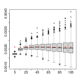
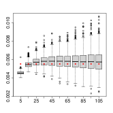
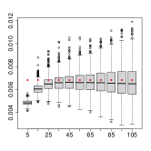
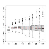
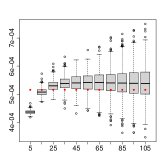
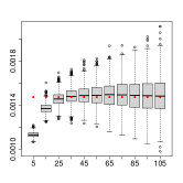
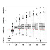
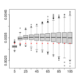
Figure 1: Boxplots of the estimated variances for the estimated recruit parameters for $W_{1}$ (upper row) and $W_{2}$ (lower row) for different truncation distances. The red dots show the empirical variance of the simulated parameter estimates.

The plots for the death parameters is depicted in Figure 9 in the Appendix B are similar to Figure 1 and with similar comments.

The plots in Figure 2 show coverage probabilities over the 1000 simulations of 95% confidence intervals based on the asymptotic normal distribution of the parameter estimates with variances estimated following Section 4. For the recruits parameters, the coverage probabilities are quite close to the nominal 95% over a wide range of truncation distances. For the death parameters, the coverage probabilities are a bit less satisfactory in case of $W_{1}$ while they get quite close to the nominal 95% in case of the bigger window $W_{2}$.

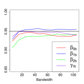
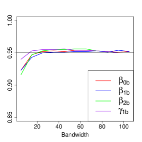
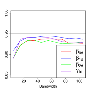
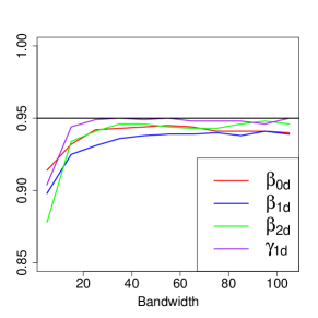
Figure 2: Coverage values for the recruits (top) and the deaths (bottom) regression parameter confidence intervals obtained with varying truncation distances and windows $W_{1}$ (left) and $W_{2}$ (right).

Overall, inference based on the asymptotic normal distribution of parameter estimates and the proposed estimates of parameter estimate variances seem reliable at least when the observation window is sufficiently large. Also, coverage probabilities of confidence intervals are fairly stable across a wide range of truncation distances which indicates a pleasing robustness to the choice of truncation distance for variance estimation.

7 The BCI data

1983	1985
1990	1995
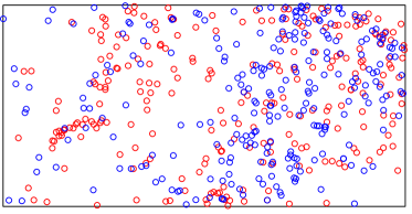
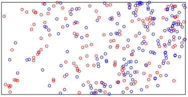
2000	2005
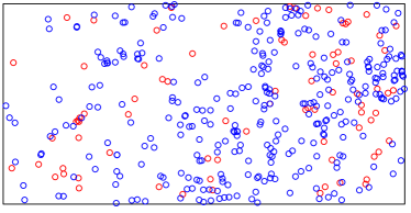
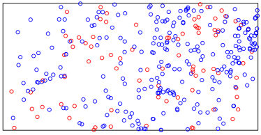
2010	2015

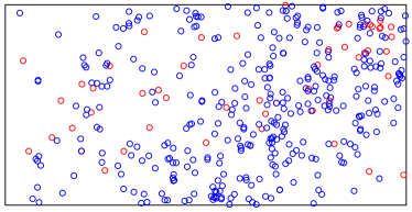
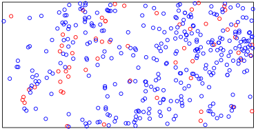
Figure 3: Spatial point patterns of locations of Capparis frondosa trees in the eight censuses of the 50 ha plot in Barro Colorado Island (BCI), Panama. Top left plot: trees in first census. Remaining plots: recruits (red) and deaths (blue) relative to previous census.

We consider tree census data from the 50 ha, $\tilde{W}=[0,1000\text{m}]\times[0,500\text{m}]$, Barro Colorado Island forest dynamics permanent study plot (Condit et al.,, 2019). The first census was conducted in 1983 and followed by 5 year interval censuses in 1985, 1990, 1995, 2000, 2005, 2010, and 2015. The censuses include all trees with diameter of breast height $m\geq 10$mm. Figure 3 shows the locations of Capparis frondosa trees in the first census and recruits and deaths for the remaining seven censuses. We here ignore that the time-interval between the first and the second census is smaller than for the remaining censuses. To some extent this is accounted for by the census dependent intercepts. Table 3 in the Appendix C summarizes the numbers of recruits and deaths in each census. The population of Capparis trees seems to be declining with a decreasing trend regarding number of recruits and increasing trend regarding number of deaths.

We employ the log linear recruit intensity function (1) with covariates interpolated copper (Cu), potassium (K), phosphorus (P), pH, mineralized nitrogen (Nmin), elevation (dem), slope gradient (grad), convergence index (convi), multi-resolution index of valley bottom flatness (mrvbf), incoming mean annual solar radiation (solar) and topographic wetness index (twi) available on a $5\times 5\,\text{m}^{2}$ grid. For the influence of existing trees we only distinguish between Capparis trees ($l=1$) and other trees ($l=2$). For the influence of Capparis on recruits we use (3) with $\psi_{1}=0.25$ and for the influence of Capparis on deaths we use (4) with $\kappa_{1}=5$. For the influence of other trees we compute influence functions of the form (4) for all abundant species other than Capparis with more than 500 trees and with $\kappa_{2}=10$. These influence functions are then averaged to get an influence function for other trees that is used both for recruits and deaths. Ideally, more refined influence functions for existing trees could be specified based on biological expertise.

The left plot in Figure 4 shows non-parametric estimates of pair correlation functions for each point pattern of recruits where the estimates are adjusted for the inhomogeneous fitted intensity functions. Despite the variability between the estimates, all estimates seem to stabilize around 1 after a distance of 55m which we use as the truncation distance for variance estimation. The middle plot shows variograms for the death events adjusted for the inhomogeneous conditional death probabilities. Based on the variograms there does not appear to be strong spatial correlation between death events and indeed our estimated standard deviations (over 40 different truncation distances) for the death regression parameter estimates are only slightly larger than the estimate obtained assuming conditionally independent death events. For the estimation of variance of the death regression parameters we use the truncation distance 55m as for the recruits. The right plot shows the intercepts for recruits that decrease over time and the intercepts for deaths that increase over time. The composite likelihood estimates of the remaining regression parameters for respectively recruits and deaths are given in Table 2 together with $Z$-scores and $p$-values.

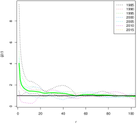
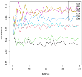
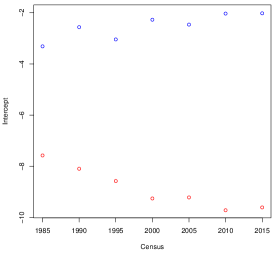
Figure 4: Left: estimated pair correlation functions for each census. Middle: variograms for death indicators for each census. Right: time dependent intercepts for recruits (blue) and deaths (red).

Table 2: Recruits (left) and death (right) parameter estimates, $Z$-scores, and $p$-values based on asymptotic normality.

	estimate	$Z$-score	$p$-value	estimate	$Z$-score	$p$-value
convi	-0.01	-3.32	0.00	-3e-3	-1.68	0.09
Cu	0.03	0.75	0.45	0.10	3.78	0.00
dem	0.02	2.21	0.03	4e-3	0.62	0.54
grad	-3.14	-2.48	0.01	0.76	0.99	0.32
K	1e-3	0.45	0.65	-2e-3	-1.38	0.17
mrvbf	-0.09	-1.48	0.14	0.02	0.47	0.64
Nmin	0.03	5.34	0.00	1e-3	0.15	0.88
P	-0.01	-0.35	0.73	-0.03	-0.99	0.32
pH	-0.21	-1.16	0.24	0.55	3.81	0.00
solar	-5e-3	-3.59	0.00	3e-3	2.70	0.01
twi	5e-3	0.12	0.91	0.03	0.87	0.39
Infl. others	0.01	1.37	0.17	-0.01	-1.27	0.21
Infl. Capparis	0.61	5.97	0.00	2e-4	0.45	0.65

We do not attempt a formal investigation of the significance of the various covariates. However, based on the $p$-values, there is some evidence that recruit intensity is negatively associated with the covariates convi and solar and positively associated with Nmin and, not surprisingly, presence of existing Capparis trees. Probability of death appears to be positively associated with high level of Cu, pH and solar. However, no dependence on existing trees is detected.

8 Discussion

Our methodology is essentially free of assumptions regarding the second-order properties of the space-time point process. However, there is an obvious risk of misspecification for the intensity and death probability regression models. This does not necessarily render regression parameter estimates meaningless. As in Choiruddin et al., (2021) one might define ‘least wrong’ regression models as those that minimize a composite likelihood Kullback-Leibler distance to the true intensity and death probability models. The composite likelihood parameter estimates are then estimates of the corresponding ‘least wrong’ regression parameter values.

We have focused on estimation of regression parameters. However, scale parameters in the models for influence of existing trees need to be determined too. If it is not possible to identify suitable values of such parameters based on biological insight, one might include these parameters as additional targets for the composite likelihood estimation. However, computations may be more cumbersome and it may be necessary to restrict maximization to a discrete set of candidate parameter values similar to what is done for irregular parameters of Markov point processes in the spatstat package.

We have not provided a theoretically well founded method for truncation distance selection for the covariance matrix estimators. Our simulation study, however, indicates robustness to the choice of truncation distance. As in the data example, plots of estimates of pair correlation functions and variograms may give some idea of suitable truncation distances.

Appendix A Second order moment density for a random variable and a point process

Consider a point process $B$ on ${\mathbb{R}}^{2}$ and a binary random variable $I(v)$ associated with the location $v\in{\mathbb{R}}^{2}$ with $P(I(v)=1)=p(v)$. Let $\lambda$ denote the intensity of $B$ and $\lambda_{I(v)}(\cdot|v)$ the conditional intensity of $B$ given $I(v)$, assuming that both intensity functions exist. Then for a non-negative function $h$,

$${\mathbb{E}}[I(v)\sum_{u\in B\cap W}h(u)]={\mathbb{E}}[I(v){\mathbb{E}}[\sum_{u\in B\cap W}h(u)\big{|}I(v)]]$$

$$= {\mathbb{E}}[I(v)\int_{W}h(u)\lambda_{I(v)}(u|v)\mathrm{d}u]=p(v)\int_{W}h(u)\lambda_{1}(u|v)\mathrm{d}u.$$

Define

$$c(u,v)=\lambda_{1}(u|v)/\lambda(u)$$

as a normalized moment density for the pair $I(v)$ and $B$. For covariances we get

$${\mathbb{C}\mathrm{ov}}[f(v)I(v),\sum_{u\in B\cap W}h(u)]=f(v)p(v)\int_{W}h(u)\lambda(u)(c(u,v)-1)\mathrm{d}u.$$

Appendix B Supplementary figures and tables for simulation study.

Figure 5 shows the covariates used for the simulation study and Figure 6 shows the evolution of the numbers of recruits and deaths for the windows $W_{1}$ and $W_{2}$.

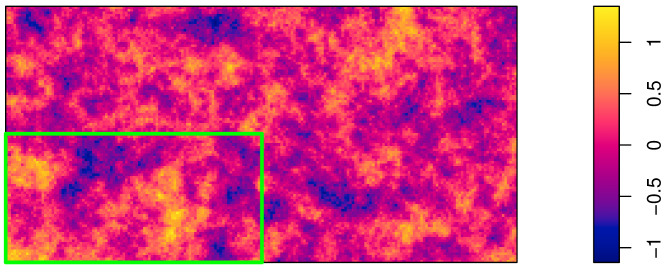
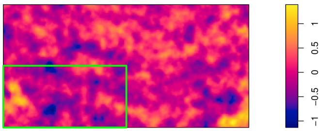
Figure 5: Covariates $Z^{(1)}$ (top) and $Z^{(2)}$ (bottom) on $W_{2}$. Green rectangle shows $W_{1}$.

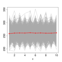
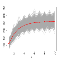
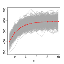
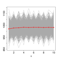
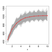
Figure 6: Gray lines show for each simulation numbers of recruits (left), numbers of deaths (middle), and the total amount of trees (right) per time step for $W_{1}$ (upper row) and $W_{2}$ (lower row). The red curves show the averages of the numbers over the 1000 simulations.

Figures 7 and 8 show histograms of the $1000$ simulated recruit and death regression parameter estimates.

$\beta_{0\mathrm{b}}$	$\beta_{1\mathrm{b}}$	$\beta_{2\mathrm{b}}$	$\gamma_{1\mathrm{b}}$

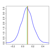
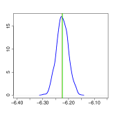
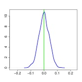
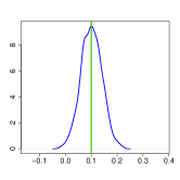
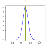
Figure 7: Histograms of simulated parameter estimates for recruits intensity for $W_{1}$ (upper row) and $W_{2}$ (lower row). Red line shows the true parameter value and green line the mean of the simulated parameter estimates.

$\beta_{0\mathrm{d}}$	$\beta_{1\mathrm{d}}$	$\beta_{2\mathrm{d}}$	$\gamma_{1\mathrm{d}}$

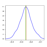
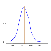
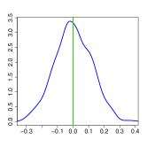
Figure 8: Histograms of simulated parameter estimates for death probabilities for $W_{1}$ (upper row) and $W_{2}$ (lower row). Red line shows the true parameter value and green line the mean of the simulated parameter estimates.

Figure 9 shows boxplots of estimates of the variances of death parameter estimates for different choices of truncation distances equivally spaced between 5 and 155m.

$\beta_{0\mathrm{d}}$	$\beta_{1\mathrm{d}}$	$\beta_{2\mathrm{d}}$	$\gamma_{1\mathrm{d}}$

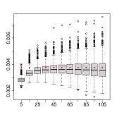
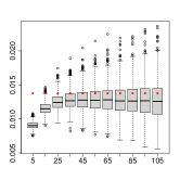
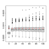
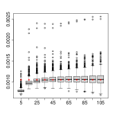
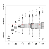
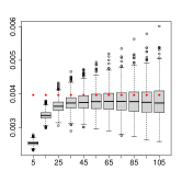
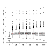
Figure 9: Boxplots of the estimated variances for the estimated death parameters using window $W_{1}$ (upper row) and $W_{2}$ (lower row) for different truncation distances. The red dots show the empirical variance of the simulated parameter estimates.

Appendix C Supplementary figures for the BCI data section

Table 3 summarizes the number of recruits and deaths in each census. The population of Capparis trees seems to be declining with a decreasing trend regarding number of recruits and increasing trend regarding number of deaths.

Table 3: Number of Capparis frondosa trees, their mean diameter at breast height, number of dead trees in the subsequent census, and number of recruits for each census conducted in the Barro Colorado Island plot.

$k$	no. trees	mean dbh	no. recruits	no. deaths
census 0	3536	21.2	—	—
census 1	3823	21.9	401	114
census 2	3823	24.5	252	252
census 3	3822	25.10	156	157
census 4	3581	26.3	82	323
census 5	3410	26.9	83	254
census 6	3107	28.1	52	355
census 7	2840	28.7	59	326

References

- Baddeley et al., (2014) Baddeley, A., Coeurjolly, J.-F., Rubak, E., and Waagepetersen, R. (2014). Logistic regression for spatial Gibbs point processes. Biometrika, 101(2):377–392.
- Baddeley et al., (2015) Baddeley, A., Rubak, E., and Turner, R. (2015). Spatial point patterns: methodology and applications with R. CRC press.
- Britton et al., (2023) Britton, T., Richards, S. A., and Hovenden, M. J. (2023). Quantifying neighbour effects on tree growth: are common ‘competition’ indices biased ? Journal of Ecology, 111:1270–1280.
- Brix and Diggle, (2001) Brix, A. and Diggle, P. J. (2001). Spatiotemporal prediction for log-Gaussian Cox processes. Journal of the Royal Statistical Society. Series B (Statistical Methodology), 63(4):823–841.
- Brix and Møller, (2001) Brix, A. and Møller, J. (2001). Space-time multi type log Gaussian Cox processes with a view to modelling weeds. Scandinavian Journal of Statistics, 28(3):471–488.
- Bullock et al., (2019) Bullock, J., González, L. M., Tamme, R., Götzenberger, L., White, S., Pärtel, M., and Hooftman, D. (2019). A synthesis of empirical plant dispersal kernels. Journal of Ecology, 105:6–19.
- Burkhart and Tomé, (2012) Burkhart, H. E. and Tomé, M. (2012). Indices of Individual-Tree Competition, pages 201–232. Springer Netherlands, Dordrecht.
- Choiruddin et al., (2021) Choiruddin, A., Coeurjolly, J.-F., and Waagepetersen, R. (2021). Information criteria for inhomogeneous spatial point processes. Australian & New Zealand Journal of Statistics, 63(1):119–143.
- Chu et al., (2022) Chu, T., Guan, Y., Waagepetersen, R., and Xu, G. (2022). Quasi-likelihood for multivariate spatial point processes with semiparametric intensity functions. Spatial Statistics, 50:100605.
- Coeurjolly and Guan, (2014) Coeurjolly, J.-F. and Guan, Y. (2014). Covariance of empirical functionals for inhomogeneous spatial point processes when the intensity has a parametric form. Journal of Statistical Planning and Inference, 155:79–92.
- Condit et al., (2019) Condit, R., Pérez, R., Aguilar, S., Lao, S., Foster, R., and Hubbell, S. (2019). Complete data from the Barro Colorado 50-ha plot: 423617 trees, 35 years. URL https://doi. org/10.15146/5xcp-0d46.
- Conley, (2010) Conley, T. G. (2010). Spatial Econometrics, pages 303–313. Palgrave Macmillan UK, London.
- Cronie and Yu, (2016) Cronie, O. and Yu, J. (2016). The discretely observed immigration-death process: likelihood inference and spatiotemporal applications. Communications in Statistics - Theory and Methods, 45(18):5279–5298.
- Crowder, (1986) Crowder, M. (1986). On consistency and inconsistency of estimating equations. Econometric Theory, 2(3):305–330.
- Diggle, (2006) Diggle, P. J. (2006). Spatio-temporal point processes, partial likelihood, foot and mouth disease. Statistical Methods in Medical Research, 15(4):325–336.
- Diggle, (2013) Diggle, P. J. (2013). Statistical analysis of spatial and spatio-temporal point patterns. CRC press.
- González et al., (2016) González, J. A., Rodríguez-Cortés, F. J., Cronie, O., and Mateu, J. (2016). Spatio-temporal point process statistics: a review. Spatial Statistics, 18:505–544.
- Häbel et al., (2019) Häbel, H., Myllymäki, M., and Pommerening, A. (2019). New insights on the behaviour of alternative types of individual-based tree models for natural forests. Ecological modelling, 406:23–32.
- Hessellund et al., (2022) Hessellund, K. B., Xu, G., Guan, Y., and Waagepetersen, R. (2022). Semiparametric multinomial logistic regression for multivariate point pattern data. Journal of the American Statistical Association, 117(539):1500–1515.
- Hiura et al., (2019) Hiura, T., Go, S., and Iijima, H. (2019). Long-term forest dynamics in response to climate change in northern mixed forests in Japan: A 38-year individual-based approach. Forest Ecology and Management, 449:117469.
- Jalilian et al., (2023) Jalilian, A., Poinas, A., Xu, G., and Waagepetersen, R. (2023). A central limit theorem for a sequence of conditionally centered and -mixing random fields. Under revision.
- Kohyama et al., (2018) Kohyama, T. S., Kohyama, T. I., and Sheil, D. (2018). Definition and estimation of vital rates from repeated censuses: Choices, comparisons and bias corrections focusing on trees. Methods in Ecology and Evolution, 9(4):809–821.
- Lavancier and Guével, (2021) Lavancier, F. and Guével, R. L. (2021). Spatial birth-death-move processes: basic properties and estimation of their intensity functions. Journal of the Royal Statistical Society Series B: Statistical Methodology, 83(4):798–825.
- May et al., (2015) May, F., Huth, A., and Wiegand, T. (2015). Moving beyond abundance distributions: neutral theory and spatial patterns in a tropical forest. Proceedings of the Royal Society B: Biological Sciences, 282(1802):20141657.
- Møller and Sørensen, (1994) Møller, J. and Sørensen, M. (1994). Statistical analysis of a spatial birth-and-death process model with a view to modelling linear dune fields. Scandinavian Journal of Statistics, 21:1–19.
- Møller and Waagepetersen, (2017) Møller, J. and Waagepetersen, R. (2017). Some recent developments in statistics for spatial point patterns. Annual Review of Statistics and Its Application, 4:317–342.
- Nathan et al., (2012) Nathan, R., Klein, E., Robledo-Arnuncio, J. J., and Revilla, E. (2012). Dispersal kernels: review. In Dispersal Ecology and Evolution. Oxford University Press.
- Pommerening and Grabarnik, (2019) Pommerening, A. and Grabarnik, P. (2019). Spatial and individual-based modelling. In Individual-based Methods in Forest Ecology and Management, pages 199–252. Springer.
- Proença-Ferreira et al., (2023) Proença-Ferreira, A., de Água, L. B., Porto, M., Mira, A., Moreira, F., and Pita, R. (2023). Dispfit: An R package to estimate species dispersal kernels. Ecological Informatics, 75:102018.
- Rasmussen et al., (2007) Rasmussen, J. G., Møller, J., Aukema, B. H., Raffa, K. F., and Zhu, J. (2007). Continuous time modelling of dynamical spatial lattice data observed at sparsely distributed times. Journal of the Royal Statistical Society. Series B (Statistical Methodology), 69(4):701–713.
- Rathbun and Cressie, (1994) Rathbun, S. L. and Cressie, N. (1994). A space-time survival point process for a longleaf pine forest in southern Georgia. Journal of the American Statistical Association, 89(428):1164–1174.
- Renshaw and Särkkä, (2001) Renshaw, E. and Särkkä, A. (2001). Gibbs point processes for studying the development of spatial-temporal stochastic processes. Computational Statistics & Data Analysis, 36(1):85–105.
- Rüger et al., (2009) Rüger, N., Huth, A., Hubbell, S. P., and Condit, R. (2009). Response of recruitment to light availability across a tropical lowland rain forest community. Journal of Ecology, 97(6):1360–1368.
- Schoenberg, (2005) Schoenberg, F. P. (2005). Consistent parametric estimation of the intensity of a spatial–temporal point process. Journal of Statistical Planning and Inference, 128(1):79–93.
- Shen et al., (2013) Shen, Y., Santiago, L. S., Ma, L., Lin, G.-J., Lian, J.-Y., Cao, H.-L., and Ye, W.-H. (2013). Forest dynamics of a subtropical monsoon forest in Dinghushan, China: recruitment, mortality and the pace of community change. Journal of Tropical Ecology, 29(2):131–145.
- Song, (2007) Song, P. X.-K. (2007). Correlated data analysis: modeling, analytics, and applications. Springer Series in Statistics. Springer, New York, NY.
- Sørensen, (1999) Sørensen, M. (1999). On asymptotics of estimating functions. Brazilian Journal of Probability and Statistics, 13:111–136.
- Waagepetersen and Guan, (2009) Waagepetersen, R. and Guan, Y. (2009). Two-step estimation for inhomogeneous spatial point processes. Journal of the Royal Statistical Society. Series B (Statistical Methodology), 71(3):685–702.
- Waagepetersen, (2007) Waagepetersen, R. P. (2007). An estimating function approach to inference for inhomogeneous Neyman–Scott processes. Biometrics, 63(1):252–258.
- White, (1980) White, H. (1980). A heteroskedasticity-consistent covariance matrix estimator and a direct test for heteroskedasticity. Econometrica, 48(4):817–838.
- Wiegand et al., (2009) Wiegand, T., Martínez, I., and Huth, A. (2009). Recruitment in tropical tree species: revealing complex spatial patterns. The American Naturalist, 174(4):E106–E140.
- Wiegand and Moloney, (2013) Wiegand, T. and Moloney, K. A. (2013). Handbook of spatial point-pattern analysis in ecology. CRC press.
- Wolf, (2005) Wolf, A. (2005). Fifty year record of change in tree spatial patterns within a mixed deciduous forest. Forest Ecology and management, 215(1-3):212–223.
- Xu et al., (2023) Xu, G., Liang, C., Waagepetersen, R., and Guan, Y. (2023). Semiparametric goodness-of-fit test for clustered point processes with a shape-constrained pair correlation function. Journal of the American Statistical Association, 118(543):2072–2087.
- Xu et al., (2019) Xu, G., Waagepetersen, R., and Guan, Y. (2019). Stochastic quasi-likelihood for case-control point pattern data. Journal of the American Statistical Association, 114(526):631–644.