Numerical Relativity Multimodal Waveforms using Absorbing Boundary Conditions

Abstract

Errors due to imperfect boundary conditions in numerical relativity simulations of binary black holes can produce unphysical reflections of gravitational waves which compromise the accuracy of waveform predictions, especially for subdominant modes. A system of higher order absorbing boundary conditions which greatly reduces this problem was introduced in earlier work Buchman and Sarbach (2006). In this paper, we devise two new implementations of this boundary condition system in the Spectral Einstein Code (SpEC), and test them in both linear multipolar gravitational wave and inspiralling mass ratio 7:1 binary black hole simulations. One of our implementations in particular is shown to be extremely robust and to produce accuracy superior to the standard freezing-$\Psi_{0}$ boundary condition usually used by SpEC.

I Introduction

With advanced LIGO-Virgo-Kagra detectors online Aasi et al. (2015); Acernese et al. (2015); Akutsu et al. (2021), and the spacecraft LISA in development Amaro-Seoane et al. (2023), the need to include accurate non-quadrupolar, subdominant modes of gravitational waves (GWs) in the waveform models produced by numerical relativity simulations becomes more and more evident. It has been reported by many publications (see, for example,  Afshordi et al. (2023); Ferguson et al. (2021); Pürrer and Haster (2020); Mehta et al. (2023); Cotesta et al. (2018); et al. (LIGO Scientific Collaboration and Collaboration); Shaik et al. (2020)) that accurate numerical relativity waveforms that include these higher-order multipoles improve both detection and parameter estimation for a variety of binary black hole (BBH) coalescing systems and their remnant properties. Such systems include unequal mass BBHs, precessing BBHs, binaries whose orbits are inclined with respect to the observer, those with certain spin alignments, and those with eccentric orbits. In Yang et al. (2023), it is shown that correct modeling of subdominant modes enables early warning and localization of GWs, which is crucial for multi-messenger astronomy. In Favata (2009); Mitman et al. (2020), the difficulty of current Cauchy codes to calculate GW non-oscillatory modes and GW memory effects properly is presented. Studies such as Joshi et al. (2023); Mills and Fairhurst (2021) show the high increase in signal-to-noise ratio as a result of including higher-order multipoles in the waveforms obtained from simulations of eccentric, spinning, BBH mergers. For the spacecraft LISA, detection of binaries with high masses and unequal mass ratios is paramount, and also depends on accurate modeling of subdominant modes Chandra et al. (2022). Finally, accurate numerical relativity multimodal waveforms will improve templates obtained using analytic effective-one-body techniques, phenomenological models, and surrogates based on reduced order modeling Islam et al. (2021); Colleoni et al. (2021).

To illustrate how subdominant modes can become important for GW modeling, we take the example of unequal mass BBHs. For these systems, the amplitudes of the subdominant $(\ell,m)$ modes relative to the dominant quadrupolar $(2,2)$ mode increase with mass ratio Buchman et al. (2012). For instance, at the frequency which gives the highest $(2,2)$ wave amplitude, the ratio of the $(3,3)$ mode amplitude to the $(2,2)$ mode amplitude increases from $0.14$ to $0.28$ as the mass ratio increases from 2:1 to 6:1 (see Figure 10 of Buchman et al. (2012)). Thus, correct calculation of gravitational waveforms for higher-order multipoles becomes increasingly critical as the mass ratio of the BBHs becomes increasingly asymmetric.

Most numerical relativity simulations do not evolve the entire spacetime out to spatial infinity, but instead truncate the domain at some artificial outer boundary at a far but finite distance from the source. The treatment of this boundary is a potential source of error. Evolving the Einstein field equations numerically on a truncated domain to obtain accurate and unique solutions is a difficult problem. Numerical and mathematical relativists have been striving for decades to formulate the Einstein equations so that the initial boundary value problem is well posed and the outer boundary conditions during the numerical evolution are constraint-preserving and, ideally, perfectly absorbing. By perfectly absorbing, we mean that the outer boundaries are completely transparent to gravitational waves passing through, including backscatter. (See Sarbach and Tiglio (2012) and the references therein for an excellent review on these topics). Achieving perfectly absorbing boundary conditions in numerical relativity is unrealistic. However, one can impose approximately absorbing boundary conditions and thus significantly reduce the spurious reflections off the outer boundary which contaminate the numerical evolution inside the grid.

A hierarchy of boundary conditions for general relativity which is perfectly absorbing for all multipoles $\ell$ of linearized gravitational radiation up to a given angular momentum number $L$ was first introduced in Buchman and Sarbach (2006). This hierarchy is referred to as a set of “higher order boundary conditions” (HOBCs), where each boundary condition order is a rung of the hierarchy, numbered by $L$. The HOBCs presented in Buchman and Sarbach (2006) are imposed on the Newman-Penrose scalar $\Psi_{0}$, and assume a Minkowski background and a spherical outer boundary. These HOBCs were subsequently improved in Buchman and Sarbach (2007), to include first-order corrections for curvature and backscatter (for quadrupolar radiation), and to be applicable to fairly general Cauchy foliations and to spherical as well as non-spherical outer boundary shapes. In this same publication, James M. Bardeen generalizes these HOBCs for all $\ell\leq L$ in the case of first order curvature corrections (but neglecting backscatter).

The standard boundary conditions used in the Spectral Einstein Code SpEC  Kidder et al. for the incoming GW degrees of freedom at the artificial outer boundary freeze the Newman-Penrose scalar $\Psi_{0}$ to its initial value. Referred to simply as “freezing-$\Psi_{0}$ boundary conditions”, they are equivalent to the lowest rung of the hierarchy ($L=1$). It is shown mathematically Buchman and Sarbach (2006) that the freezing-$\Psi_{0}$ boundary condition causes some amount of spurious reflection at the outer boundary, even for the dominant quadrupolar mode ($\ell=2$) of the GWs, while the HOBCs perfectly absorb linearized radiation for all modes with angular momentum number $\ell\leq L$. Specifically, the reflection coefficient for the freezing-$\Psi_{0}$ boundary condition decays as $(kR_{\rm bdry})^{-4}$ for every $\ell$-mode and for large $kR_{\rm bdry}$ (where $k$ is the wavenumber of the radiation and $R_{\rm bdry}$ is the radius of the outer boundary), whereas the reflection coefficients for the HOBCs are zero for $\ell\leq L$ and further, they decay as $(kR_{\rm bdry})^{-2(L+1)}$ for $\ell>L$ and for large $kR_{\rm bdry}$. (See Buchman and Sarbach (2006) for derivations of these reflection coefficients and their decay rates.) This means, for example, that the reflection coefficient for the $\ell=3$ mode decays as $(kR_{\rm bdry})^{-6}$ when the HOBC with $L=2$ is imposed, and the reflection coefficient for $\ell=4$ decays as $(kR_{\rm bdry})^{-8}$ when the HOBC with $L=3$ is imposed. It is apparent from these decay rates that spurious reflections at a specific outer boundary radius are significantly less with HOBCs than with the freezing-$\Psi_{0}$ boundary condition. The current strategy for reducing reflections in SpEC BBH simulations which utilize the freezing-$\Psi_{0}$ boundary condition is to place the outer boundary at moderately far distances (typically $R_{\rm bdry}\gtrsim 800M$). HOBCs should in principle allow for smaller $R_{\rm bdry}$’s, thus reducing the computational cost of simulations.

In Ruiz et al. (2007), it has been shown that the HOBCs presented in Buchman and Sarbach (2006) are well posed for the second-order generalized harmonic formulation of the Einstein equations, at least in the high-frequency limit (see also Kreiss and Winicour (2006); Kreiss et al. (2007)). Although not proved per se, it is likely that the HOBCs in the first order formulation are well posed as well. These HOBCs were implemented Rinne et al. (2009) for the first order generalized harmonic Cauchy formulation Lindblom et al. (2006) of the Einstein equations in SpEC as algebraic conditions on the Regge-Wheeler-Zerilli (RWZ) scalars Regge and Wheeler (1957); Zerilli (1970) in a non-rotating, single frame grid. Tests were performed with multipolar waves Rinne (2009), and the expected absorbing features were demonstrated. However, previous experience suggests that for BBH simulations, it is preferable to (i) implement the boundary conditions on the time derivative of the incoming characteristic fields and (ii) use a grid coordinate system co-moving with the binary black holes.

In this paper, we enhance the HOBC implementation of Rinne et al. (2009) for use with BBH systems. The HOBCs have been adapted for the dual-frame infrastructure of SpEC Scheel et al. (2006), and they have been recast as conditions on the time derivatives of the incoming physical characteristic modes. Regarding the latter, we have devised two natural ways of doing this. The first, corresponding to a generalization of Eq. (68) of Lindblom et al. (2006), uses information from the HOBC system to set a projection of the Weyl tensor. The second, corresponding to Equation (69) of Lindblom et al. (2006), directly sets the time derivative of the physical modes on the boundary to the prediction of the HOBC system. The former is simpler to implement, reduces exactly to the freezing-$\Psi_{0}$ condition for $L=1$, and turns out to be much more robust. Our HOBCs require that a set of auxiliary ordinary differential equations (ODEs) living on the outer boundary are integrated forward in time. These ODEs require initial conditions on the outer boundary. Accordingly, we devise a recipe for initializing these ODEs when GWs are present on the boundary at the initial time (e.g. due to junk radiation). This requires imposing the compatibility conditions that express consistency between the system of ODEs on the boundary and the metric in the interior volume near the boundary (see Sarbach and Tiglio (2012); Rauch and Massey (1974) for a review of compatibility conditions in the context of well-posed initial boundary value problems).

Our new implementations are tested both for GWs on a Minkowski background and for a mass ratio 7:1 inspiralling binary black hole system (prior to merger), and compared against the same tests using the standard $\tt SpEC$ freezing-$\Psi_{0}$ boundary condition. We calculate waveform errors due to boundary conditions by comparing waveforms extracted on the boundary with analytic solutions (for GWs on a Minkowski background) or with waveforms extracted at the same location but in simulations with more distant boundaries (for BBH simulations). We find the HOBC implementation which sets a projection of the Weyl tensor (WeylHOBC) to be superior to that which sets the time derivative of the physical modes (dtHOBC). Furthermore, the WeylHOBC implementation is found to produce higher waveform accuracy for many modes of the GWs than does the freezing-$\Psi_{0}$ boundary condition. Not all boundary-related errors are ameliorated by HOBC, however, because of currently untreated errors in the gauge modes.

Another approach presented in the literature for constructing absorbing boundary conditions is a technique called Cauchy characteristic matching (CCM) Winicour (2012); Bishop et al. (1999); Szilágyi (2000); Calabrese (2006); Ma et al. (2023). This technique combines Cauchy evolution (which is best suited for simulating the strong-field regions of spacetime York (1979)) in the interior of the domain with characteristic evolution along null hypersurfaces to future null infinity (where gravitational radiation is defined unambiguously Bondi et al. (1962); Sachs (1962); Stewart (1989)) in the exterior. Between the Cauchy and characteristic regions is a timelike interface across which information can flow in both directions. This timelike interface acts as an absorbing boundary for the interior Cauchy evolution since GW data at this boundary is obtained from the characteristic evolution. An approach much like our Weyl tensor HOBC formulation has been recently implemented in Ma et al. (2023) to achieve fully relativistic three-dimensional CCM in the numerical relativity code SpECTRE Deppe, Nils and Throwe, William and Kidder, Lawrence E. and Vu, Nils L. and others (2023). This CCM code has successfully passed several tests in non-trivial numerical relativity scenarios, but it has not yet been tried in BBH simulations. Further, it is not clear that the CCM system is well-posed since the characteristic formulation of the Einstein equations is only weakly hyperbolic Giannakopoulos et al. (2020, 2023).

Our paper is structured as follows. In Section II, we review the general HOBC formalism. In Section III, we present details of our new implementations of the boundary conditions. Results of multipolar wave tests and binary black hole inspiral simulations are presented in Section IV. Finally, in Section V we summarize our findings and suggest future improvements and applications.

Throughout this paper, Greek indices $\alpha,\beta,\ldots$ are spacetime indices, lower-case Latin indices $a,b,\ldots$ range over $t$ and $r$, and upper-case Latin indices $A,B,\ldots$ range over $\theta$ and $\phi$. Latin indices $i,j,\ldots$ from the middle of the alphabet are spatial Cartesian coordinates.

II Review

The HOBCs on the RWZ scalars $\Phi^{(\pm)}_{\ell m}$ presented in Rinne et al. (2009), as translated from those on the Newman-Penrose scalar $\Psi_{0}$ Buchman and Sarbach (2006) for the purposes of numerical relativity, are

$$[r^{2}(\partial_{t}+\partial_{r})]^{L+1}\Phi^{(\pm)}_{\ell m}\;\hat{=}\;0,$$ (1)

where $L$ is the boundary condition order. As developed in Sarbach and Tiglio (2001), the RWZ formalism (originally put forth in Regge and Wheeler (1957) and Zerilli (1970)) describes gauge-invariant gravitational perturbations of Schwarzschild spacetime, although here, we focus on the special case of a flat rather than Schwarzschild background. The RWZ scalars are denoted by $\Phi^{(\pm)}_{\ell m}$, where $\Phi^{-}_{\ell m}$ is the odd-parity Regge-Wheeler scalar, $\Phi^{+}_{\ell m}$ is the even-parity Zerilli scalar, and the subscripts $\ell,m$ refer to a spherical harmonic decomposition. They obey the following master equation for flat spacetime:

$$\left[\partial_{t}^{2}-\partial_{r}^{2}+\frac{\ell(\ell+1)}{r^{2}}\right]\Phi^{(\pm)}_{\ell m}=0.$$ (2)

The HOBCs given in Eq. (1) are perfectly absorbing for all perturbations with angular momentum numbers $\ell\leq L$. Note that Eq. (1) is the well-known Bayliss-Turkel conditions Bayliss and Turkel (1980) for the scalar wave equation.

As in reference Rinne et al. (2009), it is assumed in this paper that the metric fields can be linearized about flat spacetime close to the outer boundary, which is taken to be a sphere of constant radius $r$ (which is constant in time as well). The spacetime metric $g_{\alpha\beta}$ is written as

$$g_{\alpha\beta}=\mathring{g}_{\alpha\beta}+\delta g_{\alpha\beta},$$ (3)

and the background metric $\mathring{g}_{\alpha\beta}$ is

$$\mathring{g}=\tilde{g}_{ab}dx^{a}dx^{b}+r^{2}\hat{g}_{\text{\tiny{AB}}}dx^{\text{\tiny{A}}}dx^{\text{\tiny{B}}},$$ (4)

where $\tilde{g}=-dt^{2}+dr^{2}$ is the standard Minkowski metric on a 2-manifold $\tilde{M}$ and $\hat{g}=d\theta^{2}+\sin^{2}\theta\;d\phi^{2}$ is the standard metric on the 2-sphere. The covariant derivative compatible with the metric $\tilde{g}$ ($\hat{g}$) [$\mathring{g}$] will be denoted by $\tilde{\nabla}$ ($\hat{\nabla}$) [$\mathring{\nabla}$] and the volume element by $\tilde{\epsilon}_{ab}$ ($\hat{\epsilon}_{\text{\tiny{AB}}}$) [$\mathring{\epsilon}_{\alpha\beta\delta\gamma}$].

The RWZ scalars are computed from the spacetime metric. Thus, the metric perturbations are decomposed with respect to scalar, vector, and tensor spherical harmonics, using the basis harmonics:

$$Y_{\text{\tiny{A}}}\equiv\hat{\nabla}_{\text{\tiny{A}}}Y,~{}~{}~{}~{}S_{\text{\tiny{A}}}\equiv\hat{\epsilon}^{\text{\tiny{B}}}{}_{\text{\tiny{A}}}Y_{\text{\tiny{B}}},$$

$$Y_{\text{\tiny{AB}}}\equiv[\hat{\nabla}_{({\text{\tiny{A}}}}Y_{{\text{\tiny{B}}})}]^{\tt TT}=\hat{\nabla}_{({\text{\tiny{A}}}}\hat{\nabla}_{{\text{\tiny{B}}})}Y+{\tfrac{1}{2}}\ell(\ell+1)\hat{g}_{\text{\tiny{AB}}}Y,$$

$$S_{\text{\tiny{AB}}}\equiv\hat{\nabla}_{({\text{\tiny{A}}}}S_{{\text{\tiny{B}}})},$$ (5)

where $Y$ is the standard scalar spherical harmonic. The odd and even parity metric perturbations are treated separately (see  Rinne et al. (2009) and Sarbach and Tiglio (2001) for details). Following the gauge-invariant procedure of Sarbach and Tiglio (2001), the odd parity perturbations are

$$\delta g_{\text{\tiny{A}}b}=h_{b}S_{\text{\tiny{A}}},~{}~{}~{}~{}\delta g_{\text{\tiny{AB}}}=2kS_{\text{\tiny{AB}}},~{}~{}~{}~{}\delta g_{ab}=h_{ab}=0$$ (6)

where $h_{a}$, $k$ and $h_{ab}$ are metric amplitudes, and the even parity perturbations are

$$\delta g_{\text{\tiny{A}}b}=Q_{b}Y_{\text{\tiny{A}}},~{}~{}~{}~{}\delta g_{\text{\tiny{AB}}}=r^{2}(K\hat{g}_{\text{\tiny{AB}}}Y+GY_{\text{\tiny{AB}}}),~{}~{}~{}~{}\delta g_{ab}=H_{ab}Y$$ (7)

where again $Q_{a}$, $K$, $G$, and $H_{ab}$ are metric amplitudes. In terms of these metric amplitudes and for $\ell\geq 2$, the odd parity Regge-Wheeler scalar is

$$\Phi^{-}_{\ell m}=r\left(\dot{h}_{r}-h^{\prime}_{t}+2h_{t}/r\right)/\Lambda,$$ (8)

and the even parity Zerilli scalar is

$$\Phi^{+}_{\ell m}=\left[\Lambda^{-1}\left(2rH_{rr}-2r^{2}K^{\prime}-r^{2}\ell(\ell+1)G^{\prime}-4Q_{r}+2r^{2}G^{\prime}\right)+rK+r\ell(\ell+1)G/2-2Q_{r}+r^{2}G^{\prime}\right]/\ell(\ell+1),$$ (9)

where a dot denotes partial differentiation with respect to $t$, a prime denotes partial differentiation with respect to $r$, and $\Lambda\equiv(\ell-1)(\ell+2)$. The sign difference between Eq. (9) above and Eq. (29) of Rinne et al. (2009) allows us to match our sign conventions with those that have become standard in the numerical relativity community, as detailed in Appendix C of Boyle et al. (2019), pages 43 and 44.

As was shown in Rinne et al. (2009), the HOBCs given in Eq. (1) can be implemented numerically by introducing a set of auxiliary variables which are defined only at the boundary. These are

$$\text{w}_{k\ell m}^{(\pm)}\equiv r^{-(2k+1)}[r^{2}(\partial_{t}+\partial_{r})]^{k}\Phi^{(\pm)}_{\ell m}.$$ (10)

It was further shown in Rinne et al. (2009) that the these auxiliary variables obey a system of ODEs on the boundary, namely

$$\partial_{t}\text{w}_{k\ell m}^{(\pm)}=\frac{1}{2r^{2}}[-\ell(\ell+1)+k(k-1)]\text{w}_{(k-1)\ell m}^{(\pm)}+{\tfrac{1}{2}}\text{w}_{(k+1)\ell m}^{(\pm)}-\frac{k}{r}\text{w}_{k\ell m}^{(\pm)}.$$ (11)

This system of ODEs is closed by

$$\text{w}_{(L+1)\ell m}^{(\pm)}\;\hat{=}\;0,$$ (12)

which is equivalent to the boundary condition given by Eq. (1). Eq. (11) is integrated on the boundary for $1\leqslant k\leqslant L$, using Eq. (12) and $\text{w}_{0\ell m}^{(\pm)}=\Phi^{(\pm)}_{\ell m}/r$.

Thus, simulations with HOBCs can be carried out by evolving two coupled systems: the partial differential equations for the metric in the interior (the interior system) and the set of ODEs for $\text{w}_{k\ell m}^{(\pm)}$ on the boundary (the auxiliary system).

III Compatibility Conditions and New Formulations

The absorbing HOBCs in Rinne et al. (2009) were implemented in a single, non-rotating frame and tested for multipolar waves Rinne (2009) originating in the interior of the computational domain. The research presented in this paper extends what was done in Rinne et al. (2009) to be applicable to BBH simulations in several ways. First, the HOBC implementation has been updated for the rotating, dual-frame infrastructure of SpEC used for BBH simulations. Second, we studied cases where the values of the auxiliary variables on the boundary were nonzero at $t=0$, mimicking the initial data of BBHs which contain junk radiation. We found that in these scenarios, the auxiliary variables had to be initialized properly in order to satisfy compatibility conditions (see section III.1). Finally, the algebraic formulation presented in Rinne et al. (2009) has been modified to the form of Eq. (68) or Eq. (69) of Lindblom et al. (2006). Note that Eq. (68) of Lindblom et al. (2006) is currently used for the freezing-$\Psi_{0}$ boundary condition in SpEC. We have named the HOBC formulation derived using Eq. (68) “WeylHOBC”, and that derived using Eq. (69) “dtHOBC”. These are discussed in sections III.2.1 and III.2.2 below.

III.1 Compatibility Conditions

HOBC simulations evolve two coupled systems, interior and auxiliary, both of which provide information about the RWZ scalars $\Phi^{(\pm)}_{\ell m}$. For the two systems to be consistent, the values of $\text{w}_{k\ell m}^{(\pm)}$ evolved on the boundary should agree with the corresponding derivatives of the $\Phi^{(\pm)}_{\ell m}$ in the interior grid evaluated at the boundary. Thus, one can consider Eq. (10) as a constraint establishing the compatibility of the two systems, a constraint known as a compatibility condition (see Sec. 5 of Sarbach and Tiglio (2012)). We must initialize $\text{w}_{k\ell m}^{(\pm)}$ correctly for the compatibility condition to be satisfied at $t=0$.

We introduce the null coordinates $v=t+r$ and $u=t-r$ to parameterize the numerical solution for the differential operator in Eq. (10). In these coordinates, the differential operator $r^{2}(\partial_{t}+\partial_{r})$ represents a directional derivative along a path of constant $u$. For a general choice of parameter $\lambda(v)$ labeling points on this path, the corresponding tangent vector will be given by

$$\left.\frac{\partial}{\partial\lambda}\right|_{u}=\left.\frac{\partial r}{\partial\lambda}\right|_{u}(\partial_{r}+\partial_{t}).$$ (13)

For appropriate choice of $\lambda(r)$, namely that for which $\left.\partial r/\partial\lambda\right|_{u}=r^{2}$, the derivative $d/d\lambda$ will be the differential operator $r^{2}(\partial_{t}+\partial_{r})$ in Eq.(10). Solving for $\lambda(r)$,

$$\lambda=-\frac{1}{r}.$$ (14)

We then utilize Eq. (13) on our boundary condition formulation to solve for the initialization of the auxiliary variables.

$$\text{w}_{k\ell m}^{(\pm)}\equiv r^{-(2k+1)}\left(\frac{\partial}{\partial\lambda}\right)^{k}\Phi^{(\pm)}_{\ell m}.$$ (15)

Our goal now is to gather $\Phi^{(\pm)}_{\ell m}(\lambda)$ for particular events along a line of constant $u$. This involves running a short-time Cauchy evolution on a larger grid extending beyond the desired boundary location. The larger grid for the short run is chosen to have an outer boundary sufficiently distant from our desired outer boundary so as to remain out of causal contact throughout the short run. Since the outer boundary of the short run does not matter, it can use the $L=1$ (freezing-$\Psi_{0}$) boundary condition which does not depend on initialization of $\text{w}_{k\ell m}^{(\pm)}$. Subsequently, we measure $\Phi^{(\pm)}_{\ell m}$ at several values of $\lambda$ from the short run, and perform a polynomial fit to $\Phi^{(\pm)}_{\ell m}(\lambda)$:

$$\Phi^{(\pm)}_{\ell m}(\lambda)=\sigma_{0}+\sigma_{1}\lambda+\sigma_{2}\lambda^{2}+\sigma_{3}\lambda^{3}.$$ (16)

The Python scipy.optimize.curvefit function is employed to determine $\sigma_{i}$ ($i=$0,1,2,3) for achieving a least squares best fit. Subsequently, we evaluate $\text{w}_{k\ell m}^{(\pm)}$ using Eq.(15) in conjunction with Eq.(16).

Recall that our HOBC (Eq. (1)) is equivalent to $\text{w}_{(L+1)\ell m}^{(\pm)}=0$ (Eq. (12)). However, whereas $\text{w}_{(L+1)\ell m}^{(\pm)}=0$ is enforced in the auxiliary system, the corresponding condition on the derivatives of $\Phi^{(\pm)}_{\ell m}$ is not imposed in the interior evolution. So the enforcement of Eq. (12) at each timestep and for each $\ell$, $m$, and parity is at least somewhat inconsistent with with the compatibility condition given in Eq. (10). One might impose the compatibility condition for order $(L+1)$ by setting $\text{w}_{(L+1)\ell m}^{(\pm)}=g(t)$, where $g(t=0)\equiv g_{0}$ is determined by the volume data metric evaluated on the boundary for the initial time. The time dependence must then be specified explicitly. Setting $g$ to a constant is undesirable, since then the wave passing through at $t=0$ would leave a permanent imprint on the boundary. A better alternative might be to damp this initial wave exponentially by employing something of the form $g(t)=g_{0}e^{-t/\tau}$. This still will not guarantee satisfaction of the compatibility condition for $\text{w}_{(L+1)\ell m}^{(\pm)}$ at later times. It can be argued that if $\text{w}_{(L+1)\ell m}^{(\pm)}$ is dynamically significant, it is advisable to evolve the HOBC auxiliary system to an order of at least $(L+1)$. In all cases we have investigated, we have found that the magnitude of $\text{w}_{k\ell m}^{(\pm)}$ decreases rapidly with $k$, usually approaching machine double precision by $k=4$, and furthermore, that the computational cost of increasing $L$ to this value (or higher) is negligible. Consequently, we always set $g_{0}=0$.

III.2 New Higher Order Boundary Condition Formulations

In the first order generalized harmonic formulation of the Einstein equations Lindblom et al. (2006) used by SpEC, there are three types of characteristic fields which require outer boundary conditions: constraint, physical, and gauge. As presented in Lindblom et al. (2006), constraint-preserving, freezing-$\Psi_{0}$, and constant-in-time gauge boundary conditions are the current standard in SpEC. In this paper, we focus on improving the boundary conditions for the characteristic fields representing physical gravitational waves. We start by outlining the mathematical description of these physical modes incoming at the outer boundary. They are given in Eq. (33) of Lindblom et al. (2006) as

$$u^{1-}_{\alpha\beta}=\Pi_{\alpha\beta}-n^{i}\Phi_{i\alpha\beta}-\gamma_{2}g_{\alpha\beta},$$ (17)

where

$$\Pi_{\alpha\beta}\equiv-t^{\gamma}\partial_{\gamma}g_{\alpha\beta}~{}~{}~{}~{}{\rm and}~{}~{}~{}~{}\Phi_{i\alpha\beta}\equiv\partial_{i}g_{\alpha\beta}.$$ (18)

In these equations, $\gamma_{2}$ is a parameter arising from the addition of constraint-damping terms to the evolution equations, $n^{\alpha}$ is the outward-pointing unit spacelike normal to the boundary on the $t=$ constant slices, and $t^{\alpha}$ is the future directed unit timelike normal to the $t=$ constant surfaces ($t^{\alpha}n_{\alpha}=0$).

In order to cast Eq. (17) in terms of covariant derivatives with respect to the background metric instead of partial derivatives (which depend on the coordinate system), we introduce the outgoing and incoming null vectors as $\ell^{\alpha}\equiv(t^{\alpha}+n^{\alpha})$ and $k^{\alpha}\equiv(t^{\alpha}-n^{\alpha})$, respectively, and let $\mathring{\nabla}_{\ell}\equiv\ell^{\alpha}\mathring{\nabla}_{\alpha}$ denote covariant differentiation along $\ell^{\alpha}$. A simple partial derivative operator $(\partial_{t}+\partial_{r})$ will be denoted by $D$. The incoming characteristic fields at the boundary can then be expressed as

$$u^{1-}_{\alpha\beta}=-(\mathring{\nabla}_{\ell}+\gamma_{2})g_{\alpha\beta}.$$ (19)

Note that the introduction of a flat-space covariant derivative in Eq. (19) simplifies the transformation to spherical-polar coordinates.

Given that the 2-metric intrinsic to the boundary is $P_{\alpha\beta}\equiv g_{\alpha\beta}+t_{\alpha}t_{\beta}-n_{\alpha}n_{\beta}$, the projection operator for the boundary conditions on the two physical degrees of freedom is $P^{\mathrm{P}}_{\alpha\beta}{}^{\gamma\delta}=P_{\alpha}{}^{\gamma}P_{\beta}{}^{\delta}-{\tfrac{1}{2}}P_{\alpha\beta}P^{\gamma\delta}$, where $P^{\mathrm{P}}_{\alpha\beta}{}^{\gamma\delta}$ constructs the transverse-traceless version of a symmetric spacetime tensor. Given that only the perturbation of the metric is involved, the projection is onto the background geometry which in this case is the 2-sphere. The resulting non-zero components of the physical boundary conditions are then the angular components:

$$u^{1-}_{\text{\tiny{AB}}}~{}\hat{=}~{}P^{\mathrm{P}}_{\text{\tiny{AB}}}{}^{\gamma\delta}u^{1-}_{\gamma\delta}=-r^{2}(\partial_{t}+\partial_{r})(r^{-2}\delta g^{\tt TT}_{\text{\tiny{AB}}})-\gamma_{2}\;\delta g^{\tt TT}_{\text{\tiny{AB}}},$$ (20)

where $\tt TT$ denotes the trace-free part with respect to the metric $\hat{g}$ on the 2-sphere and $\hat{=}$ indicates “at the boundary”.

In Rinne et al. (2009), HOBCs are imposed using the auxiliary system of $\text{w}_{k\ell m}^{(\pm)}$’s to specify the fields $u_{\text{\tiny{AB}}}^{1-}$ on the boundary, according to Eqs. (46) and (50) of that paper. This was shown in Rinne et al. (2009) to be successful when the multipolar wave initial data was zero on the boundary. However, in the general binary black hole case, there is non-zero GW data on the boundary initially. As discussed in Kidder et al. (2005) and Lindblom et al. (2006), discontinuities produced with an algebraic boundary condition are avoided by casting the boundary condition in a time-derivative form as per Bjørhus Bjørhus (1995). Hence the boundary conditions which we present in the next two sections are represented by

$$d_{t}u^{1-}_{\text{\tiny{AB}}}\hat{=}~{}P^{\mathrm{P}}_{\text{\tiny{AB}}}{}^{\gamma\delta}\partial_{t}u^{1-}_{\gamma\delta}.$$ (21)

Reference Lindblom et al. (2006) presents two ways to implement such time derivative physical boundary conditions in Eqs. (68) and (69), reproduced here for clarity. Utilizing our notation, Eq. (68) of Lindblom et al. (2006) is

$$d_{t}u^{1-}_{\text{\tiny{AB}}}\hat{=}~{}P^{\mathrm{P}}_{\text{\tiny{AB}}}{}^{\gamma\delta}[D_{t}u^{1-}_{\gamma\delta}+v(\omega_{\gamma\delta}-\omega_{\gamma\delta}|_{\text{\tiny{BC}}}-\gamma_{2}n^{i}c^{3}_{i\gamma\delta})],$$ (22)

where the quantity $D_{t}u$ is the right hand side of the first order generalized harmonic evolution system, $v$ is the characteristic speed at which the characteristic field $u^{1-}_{\alpha\beta}$ enters the boundary, $\omega_{\gamma\delta}$ is the projection of the Weyl tensor, $\omega_{\gamma\delta}|_{\text{\tiny{BC}}}$ is the target value to which $\omega_{\gamma\delta}$ is to be fixed at the boundary, and $n^{i}c^{3}_{i\gamma\delta}$ are incoming constraint fields (see Lindblom et al. (2006) for more details). Eq. (69) of Lindblom et al. (2006) is

$$d_{t}u^{1-}_{\text{\tiny{AB}}}\hat{=}~{}P^{\mathrm{P}}_{\text{\tiny{AB}}}{}^{\gamma\delta}\dot{h}_{\gamma\delta}(t,r),$$ (23)

where $\dot{h}_{\gamma\delta}(t,r)$ is a pre-determined waveform ($\dot{x}\equiv\partial_{t}{x}$). The precise form of these conditions and their interface with the auxiliary system will be described in the two sections below. The WeylHOBC formulation uses the auxiliary system to set a projection of the Weyl tensor and is equivalent to using the time derivative of $u^{1-}$ to drive the radial derivative of $u^{1-}$ at the boundary to a desired value. The dtHOBC formulation directly sets the time derivative of the incoming physical field to its value in the auxiliary system.

III.2.1 WeylHOBC Formulation

The incoming wave projection of the Weyl tensor contains the information needed to construct the physical boundary conditions, as proposed in Bardeen and Buchman (2002). These ideas as well as those in Reula and Sarbach (2005) were adapted for the 3D Einstein equations in Kidder et al. (2005) and further developed for the first order generalized harmonic system in Lindblom et al. (2006).

The goal of this section is to calculate the quantity $\omega_{\gamma\delta}|_{\text{\tiny{BC}}}$ of Eq. (22). To begin, recall

$$\omega_{\alpha\beta}=P^{\mathrm{P}}_{\alpha\beta}{}^{\varepsilon\zeta}~{}C_{\varepsilon\mu\zeta\nu}\;\ell^{\mu}\ell^{\nu},$$ (24)

where $C_{\varepsilon\mu\zeta\nu}$ is the Weyl tensor. Since a vacuum background is assumed and since the projection operator selects only the angular components, Eq. (24) becomes

$$\omega_{\text{\tiny{AB}}} = P^{\mathrm{P}}_{\text{\tiny{AB}}}{}^{\varepsilon\zeta}~{}R_{\varepsilon\mu\zeta\nu}\;\ell^{\mu}\ell^{\nu}$$ (25)

$$= \left(R_{\text{\tiny{A}}\mu\text{\tiny{B}}\nu}-{\tfrac{1}{2}}R^{\text{\tiny{C}}}_{\;\mu{\text{\tiny{C}}}\nu}P_{\text{\tiny{AB}}}\right)\ell^{\mu}\ell^{\nu},$$ (26)

where $R_{\varepsilon\mu\zeta\nu}$ is the Riemann tensor and $P_{\text{\tiny{AB}}}=r^{2}\hat{g}_{\text{\tiny{AB}}}$. In terms of metric perturbations with respect to the flat spacetime metric in Eq. (4), Eq. (26) becomes

$$\begin{split}\omega_{\text{\tiny{AB}}}={\tfrac{1}{2}}\;\ell^{\nu}\ell^{\mu}\;\bigl{[}\hat{\nabla}_{\text{\tiny{B}}}\mathring{\nabla}_{\nu}\;\delta g_{\text{\tiny{A}}\mu}+\mathring{\nabla}_{\mu}\hat{\nabla}_{\text{\tiny{A}}}\;\delta g_{\text{\tiny{B}}\nu}-\hat{\nabla}_{\text{\tiny{B}}}\hat{\nabla}_{\text{\tiny{A}}}\;\delta g_{\mu\nu}-\mathring{\nabla}_{\nu}\mathring{\nabla}_{\mu}\;\delta g_{\text{\tiny{AB}}}\\ -{\tfrac{1}{2}}\bigl{(}\hat{\nabla}_{\text{\tiny{C}}}\mathring{\nabla}_{\nu}\;\delta g^{\text{\tiny{C}}}_{~{}\mu}+\mathring{\nabla}_{\mu}\hat{\nabla}_{\text{\tiny{C}}}\;\delta g^{\text{\tiny{C}}}_{~{}\nu}-\hat{\nabla}_{\text{\tiny{C}}}\hat{\nabla}^{\text{\tiny{C}}}\;\delta g_{\mu\nu}-\mathring{\nabla}_{\mu}\mathring{\nabla}_{\nu}\;\delta g^{\text{\tiny{C}}}_{~{}{\text{\tiny{C}}}}\bigr{)}r^{2}\hat{g}_{\text{\tiny{AB}}}\bigr{]}.\end{split}$$ (27)

After a lengthy calculation, Eq. (27) can be simplified for general parity. Recalling $\mathring{\nabla}_{\ell}\equiv\ell^{\varepsilon}\mathring{\nabla}_{\varepsilon}$ (note that $\ell$ is not an index) and $D=(\partial_{t}+\partial_{r})$, the result is

$$\begin{split}\omega_{\text{\tiny{AB}}}={\tfrac{1}{2}}\bigl{[}\hat{\nabla}_{\text{\tiny{B}}}\mathring{\nabla}_{\ell}\{\delta g_{\text{\tiny{A}}\mu}\ell^{\mu}\}+\hat{\nabla}_{\text{\tiny{A}}}\mathring{\nabla}_{\ell}\{\delta g_{\text{\tiny{B}}\mu}\ell^{\mu}\}-r^{-2}\mathring{\nabla}_{\ell}\{r^{2}\mathring{\nabla}_{\ell}\;\delta g_{\text{\tiny{AB}}}\}-\hat{\nabla}_{\text{\tiny{B}}}\hat{\nabla}_{\text{\tiny{A}}}\{\delta g_{\mu\nu}\ell^{\mu}\ell^{\nu}\}+\frac{1}{r}\left(\hat{\nabla}_{\text{\tiny{B}}}\left\{\delta g_{\text{\tiny{A}}\mu}\ell^{\mu}\right\}+\hat{\nabla}_{\text{\tiny{A}}}\left\{\delta g_{\text{\tiny{B}}\mu}\ell^{\mu}\right\}\right)~{}~{}~{}~{}~{}~{}\\ -{\tfrac{1}{2}}\left(2\hat{\nabla}^{\text{\tiny{C}}}\mathring{\nabla}_{\ell}\{\delta g_{\text{\tiny{C}}\mu}\ell^{\mu}\}-r^{-2}\mathring{\nabla}_{\ell}\{r^{2}\mathring{\nabla}_{\ell}\;\delta g_{\;\text{\tiny{C}}}^{\text{\tiny{C}}}\}-\hat{\nabla}_{\text{\tiny{C}}}\hat{\nabla}^{\text{\tiny{C}}}\{\delta g_{\mu\nu}\ell^{\mu}\ell^{\nu}\}+\frac{2}{r}\hat{\nabla}^{\text{\tiny{C}}}\{\delta g_{\text{\tiny{C}}\mu}\ell^{\mu}\}\right)r^{2}\hat{g}_{\text{\tiny{AB}}}\bigr{]}.~{}~{}~{}~{}~{}~{}~{}~{}~{}~{}~{}~{}~{}~{}~{}~{}~{}~{}~{}~{}~{}~{}~{}~{}~{}~{}~{}~{}~{}~{}~{}~{}~{}~{}~{}~{}~{}~{}\end{split}$$ (28)

Specialization to odd and even parity GW metric perturbations, given the auxiliary variables $\text{w}_{k\ell m}^{(\pm)}$ and the vacuum linearized Einstein equations, is shown in sections III.2.1.1 and III.2.1.2. The expressions then obtained for odd and even parity $\omega_{\text{\tiny{AB}}}^{\pm}$are used as the target values $\omega^{\pm}_{\text{\tiny{AB}}}|_{\text{\tiny{BC}}}$.

III.2.1.1 Odd Parity

Substituting the odd parity metric perturbations of Eq. (6) into Eq. (28), one obtains

$$\begin{split}\omega^{-}_{\text{\tiny{AB}}}={\tfrac{1}{2}}\bigl{[}\hat{\nabla}_{\text{\tiny{B}}}\mathring{\nabla}_{\ell}\{h_{a}\ell^{a}S_{\text{\tiny{A}}}\}+\hat{\nabla}_{\text{\tiny{A}}}\mathring{\nabla}_{\ell}\{h_{a}\ell^{a}S_{\text{\tiny{B}}}\}-r^{-2}\mathring{\nabla}_{\ell}\bigl{(}r^{2}\mathring{\nabla}_{\ell}\{2kS_{\text{\tiny{AB}}}\}\bigr{)}+\frac{1}{r}\bigl{(}\hat{\nabla}_{\text{\tiny{B}}}\{h_{a}\ell^{a}S_{\text{\tiny{A}}}\}+\hat{\nabla}_{\text{\tiny{A}}}\{h_{a}\ell^{a}S_{\text{\tiny{B}}}\}\bigr{)}~{}~{}~{}~{}~{}~{}~{}~{}~{}~{}~{}~{}~{}~{}~{}~{}~{}~{}~{}~{}\\ -{\tfrac{1}{2}}\left(2\hat{\nabla}^{\text{\tiny{C}}}\mathring{\nabla}_{\ell}\{h_{a}\ell^{a}S_{\text{\tiny{C}}}\}-r^{-2}\mathring{\nabla}_{\ell}\bigl{(}r^{2}\mathring{\nabla}_{\ell}\{2kS_{\;\text{\tiny{C}}}^{\text{\tiny{C}}}\}\bigr{)}+\frac{2}{r}\hat{\nabla}^{\text{\tiny{C}}}\{h_{a}\ell^{a}S_{\text{\tiny{C}}}\}\right)r^{2}\hat{g}_{\text{\tiny{AB}}}\bigr{]}.~{}~{}~{}~{}~{}~{}~{}~{}~{}~{}~{}~{}~{}~{}~{}~{}~{}~{}~{}~{}~{}~{}~{}~{}~{}~{}~{}~{}~{}~{}~{}~{}~{}~{}~{}~{}~{}~{}~{}~{}~{}~{}~{}~{}~{}~{}~{}~{}~{}~{}~{}~{}~{}~{}~{}~{}~{}~{}~{}\end{split}$$ (29)

Expansion of the last (trace) term of Eq. (29) yields terms involving $\hat{\nabla}_{\text{\tiny{C}}}(h_{a}\ell^{a})$, $\hat{\nabla}_{\text{\tiny{C}}}S^{\text{\tiny{C}}}$ and $S_{\text{\tiny{C}}}^{\;\text{\tiny{C}}}$ which equal zero with the result that this last term vanishes. Further expansion and subsequent simplification of Eq. (29) gives

$$\omega^{-}_{\text{\tiny{AB}}}=\left[D\left(h_{a}\ell^{a}\right)+\frac{2}{r}Dk-\frac{2}{r^{2}}k-D^{2}k\right]S_{\text{\tiny{AB}}}.$$ (30)

The auxiliary variables as defined in Eq. (10), are now introduced through the term $D^{2}k$. Using Eq. (45) of Rinne et al. (2009) to relate $Dk$ to the auxiliary variables and using Eq. (8) of Rinne et al. (2009) to find expressions for $D\text{w}_{0\ell m}^{-}$ and $D\text{w}_{1\ell m}^{-}$, we obtain

$$D^{2}k=D\left(h_{a}\ell^{a}\right)+\frac{2}{r}Dk-\frac{2}{r^{2}}k+r^{2}\text{w}_{2\ell m}^{-}.$$ (31)

One can see by inspection that substituting Eq. (31) into Eq. (30) gives the final simple and elegant result for odd parity:

$$\omega^{-}_{\text{\tiny{AB}}}=-r^{2}\text{w}_{2\ell m}^{-}\;S_{\text{\tiny{AB}}}.$$ (32)

This value will now be used for the odd parity target value, $\omega^{-}_{\text{\tiny{AB}}}|_{\text{\tiny{BC}}}$.

III.2.1.2 Even Parity

Specializing Eq. (28) to even parity using the perturbations given in Eq. (7), one obtains

$$\omega_{\text{\tiny{AB}}} = {\tfrac{1}{2}}\;\bigl{[}\hat{\nabla}_{\text{\tiny{B}}}\left(\mathring{\nabla}_{\ell}\{\ell^{a}Q_{a}Y_{\text{\tiny{A}}}\}\right)+\hat{\nabla}_{\text{\tiny{A}}}\left(\mathring{\nabla}_{\ell}\{\ell^{a}Q_{a}Y_{\text{\tiny{B}}}\}\right)-r^{-2}\mathring{\nabla}_{\ell}\bigl{(}r^{2}\mathring{\nabla}_{\ell}\{K\hat{g}_{\text{\tiny{AB}}}\;Y+G\;Y_{\text{\tiny{AB}}}\}\bigr{)}$$

$$-\hat{\nabla}_{\text{\tiny{B}}}\hat{\nabla}_{\text{\tiny{A}}}\left\{H_{ab}\ell^{a}\ell^{b}\;Y\right\}+\frac{1}{r}\left(\hat{\nabla}_{\text{\tiny{B}}}\left\{\ell^{a}Q_{a}Y_{\text{\tiny{A}}}\right\}+\hat{\nabla}_{\text{\tiny{A}}}\left\{\ell^{a}Q_{a}Y_{\text{\tiny{B}}}\right\}\right)\bigr{]}^{\tt TT}.$$

Note here that it was found to be more straightforward to take the transverse-traceless part of each term rather than to explicitly subtract the trace as in Eq. (28). Doing so and simplifying gives

$$\omega_{\text{\tiny{AB}}}={\tfrac{1}{2}}\left[2D(\ell^{a}Q_{a})-D(r^{2}DG)-H_{ab}\ell^{a}\ell^{b}\right]Y_{\text{\tiny{AB}}}$$ (34)

To make things simpler, we turn to the generalized Regge-Wheeler gauge with the idea that if the results are true in one gauge, they are true in all gauges since the expression is gauge invariant. The generalized Regge-Wheeler gauge is defined so that $Q_{b}$ and $G$ of Eq. (7) vanish (see Sarbach and Tiglio (2001) page 4). Also, in this gauge, $H_{ab}$ and $K$ correspond with their gauge-invariant counterparts, $H^{(inv)}_{ab}$ and $K^{(inv)}$ for $\ell>2$. Thus in the Regge-Wheeler gauge and for $\ell>2$, Eq. (34) simplifies to

$$\omega_{\text{\tiny{AB}}}=-{\tfrac{1}{2}}\;H^{(inv)}_{ab}\ell^{a}\ell^{b}\;Y_{\text{\tiny{AB}}}.$$ (35)

In order to introduce the auxiliary variables $\text{w}_{2\ell m}^{+}$, we make use of Eq. (19) of Buchman and Sarbach (2007), which relates $H^{(inv)}_{ab}$ to the even parity Zerilli scalar $\Phi_{\ell m}^{+}$ via

$$H^{(inv)}_{ab}=2\bigl{(}\tilde{\nabla}_{a}\tilde{\nabla}_{b}-{\tfrac{1}{2}}\tilde{g}_{ab}\tilde{\nabla}^{d}\tilde{\nabla}_{d}\bigr{)}r\Phi_{\ell m}^{+}.$$ (36)

Again, the sign difference from Eq. (19) of Buchman and Sarbach (2007) makes the sign of $\Phi_{\ell m}^{+}$ agree with the usual sign conventions in numerical relativity, as mentioned earlier. Plugging into Eq. (35), one gets

$$\omega_{\text{\tiny{AB}}}=-\left[\bigl{(}\tilde{\nabla}_{a}\tilde{\nabla}_{b}-{\tfrac{1}{2}}\tilde{g}_{ab}\tilde{\nabla}^{d}\tilde{\nabla}_{d}\bigr{)}r\Phi_{\ell m}^{+}\right]\ell^{a}\ell^{b}\;Y_{\text{\tiny{AB}}},$$ (37)

which simplifies to $\omega_{\text{\tiny{AB}}}=-D^{2}(r\Phi_{\ell m}^{+})Y_{\text{\tiny{AB}}}$ noting that $\tilde{g}_{ab}\ell^{a}\ell^{b}=0$ for Minkowski spacetime. This expression is gauge invariant provided the derivatives of $\Phi_{\ell m}^{+}$ are gauge invariant. Using the equation for $\text{w}^{+}_{2\ell m}$ obtained from Eq. (10), namely

$$r^{2}\text{w}^{+}_{2\ell m}=r^{-1}D\bigl{[}r^{2}D\Phi_{\ell m}^{+}\bigr{]}=D^{2}(r\Phi_{\ell m}^{+}),$$ (38)

one again arrives at a wonderfully simple result:

$$\omega^{+}_{\text{\tiny{AB}}}=-r^{2}\text{w}^{+}_{2\ell m}\;Y_{\text{\tiny{AB}}}.$$ (39)

This is the value that will be used for the even parity target value, $\omega^{+}_{\text{\tiny{AB}}}|_{\text{\tiny{BC}}}$.

III.2.2 dtHOBC Formulation

In this section, the HOBCs are implemented via Eq. (23), where $\dot{h}_{\alpha\beta}=\partial_{t}u^{1-}_{\alpha\beta}$. The result is

$$d_{t}u^{1-}_{\text{\tiny{AB}}}\;\hat{=}\;P^{\mathrm{P}}_{\text{\tiny{AB}}}{}^{\gamma\delta}\left(\partial_{t}{u}^{1-}_{\gamma\delta}\right)=-P^{\mathrm{P}}_{\text{\tiny{AB}}}{}^{\gamma\delta}r^{2}(\partial_{t}^{2}+\partial_{t}\partial_{r})(r^{-2}\delta g_{\gamma\delta})-\gamma_{2}P^{\mathrm{P}}_{\text{\tiny{AB}}}{}^{\gamma\delta}\;\partial_{t}\delta g_{\gamma\delta}.$$ (40)

Notice that the $\gamma_{2}$ term is annihilated by $P^{\mathrm{P}}_{\alpha\beta}{}^{\gamma\delta}$ in the algebraic boundary condition implemented in Rinne et al. (2009), but not in the corresponding time-derivative boundary condition.

Since $P_{\text{\tiny{AB}}}=r^{2}\hat{g}_{\text{\tiny{AB}}}$, it follows that $P^{\mathrm{P}}_{\text{\tiny{AB}}}{}^{\gamma\delta}=P_{\text{\tiny{A}}}{}^{\gamma}P_{\text{\tiny{B}}}{}^{\delta}-(r^{2}/2)\hat{g}_{\text{\tiny{AB}}}P^{\gamma\delta}$. Also keeping in mind that $P^{\text{\tiny{AB}}}=r^{-2}\hat{g}^{\text{\tiny{AB}}}$ and $P_{\text{\tiny{A}}}^{\,{\text{\tiny{B}}}}=\delta_{\text{\tiny{A}}}^{\,{\text{\tiny{B}}}}$, we obtain

$$d_{t}u^{1-}_{\text{\tiny{AB}}} \;\hat{=}\; -r^{2}(\partial_{t}^{2}+\partial_{t}\partial_{r})(r^{-2}\delta g_{\text{\tiny{AB}}}^{\tt TT})-\gamma_{2}\;\partial_{t}\delta g_{\text{\tiny{AB}}}^{\tt TT}$$ (41)

Expressions for the right-hand-side of Eq. (41) are derived in the Regge-Wheeler-Zerilli formalism which involve the auxiliary variables at the boundary.

III.2.2.1 Odd Parity

The gauge-invariant potential $h^{(\mathrm{inv})}$ Sarbach and Tiglio (2001) is related to the odd parity Regge-Wheeler scalar $\Phi_{\ell m}^{-}$ via $h^{(\mathrm{inv})}=\tilde{*}{\rm d}(r\Phi_{\ell m}^{-})$, where $\tilde{*}$ denotes the Hodge dual with respect to $\tilde{g}$. In particular, $\tilde{*}u_{a}dx^{a}=\tilde{\epsilon}_{ab}u^{a}dx^{b}$ (from the top of page 3 of Sarbach and Tiglio (2001)), where $\tilde{\epsilon}_{ab}$ is the standard volume element in $(\tilde{M},\tilde{g})$, oriented so that $\tilde{\epsilon}_{tr}=|\tilde{g}|^{1/2}$. For flat spacetime, $\tilde{\epsilon}_{tr}=-\tilde{\epsilon}_{rt}=1$, and $\tilde{\epsilon}^{\,tr}=-\tilde{\epsilon}^{\,rt}=-1$. Applying this to the expression $h^{(\mathrm{inv})}=\tilde{*}{\rm d}(r\Phi_{\ell m}^{-})$, we obtain

$$h^{(\mathrm{inv})}=~{}~{}\tilde{\epsilon}_{ab}\;\partial^{a}(r\Phi_{\ell m}^{-})dx^{b}=-\partial_{t}(r\Phi_{\ell m}^{-})dr-\partial_{r}(r\Phi_{\ell m}^{-})dt.$$ (42)

Since the 1-form $h^{(\mathrm{inv})}$ is decomposed as $h^{(\mathrm{inv})}=h^{(\mathrm{inv})}_{r}dr+h^{(\mathrm{inv})}_{t}dt$, it follows that

$$h_{r}^{(\mathrm{inv})}=-\partial_{t}(r\Phi_{\ell m}^{-})~{}~{}~{}~{}{\text{and}}~{}~{}~{}~{}h_{t}^{(\mathrm{inv})}=-\partial_{r}(r\Phi_{\ell m}^{-}).$$ (43)

Using Eqs. (16) and (17) of Rinne et al. (2009), which are $h^{(\mathrm{inv})}_{t}=h_{t}-\partial_{t}k$ and $h^{(\mathrm{inv})}_{r}=h_{r}-r^{2}\partial_{r}(r^{-2}k)$, respectively, we re-express the time-derivative boundary condition (41) in terms of the amplitudes $h_{a}$ and the odd-parity auxiliary variables $\text{w}_{k\ell m}^{-}$ to give

$$(\partial_{t}+\partial_{r})(r^{-2}k)=r^{-2}(h_{t}+h_{r}+r^{2}\text{w}_{1\ell m}^{-}+r\text{w}_{0\ell m}^{-}).$$ (44)

With $\delta g_{\text{\tiny{AB}}}^{\tt TT}=2kS_{\text{\tiny{AB}}}$ Rinne et al. (2009), substitution into Eq. (41) gives

$$d_{t}u^{1-}_{\text{\tiny{AB}}}\;\hat{=}\;-2[\dot{h}_{t}+\dot{h}_{r}+r^{2}\dot{\text{w}}_{1\ell m}^{-}+r\dot{\text{w}}_{0\ell m}^{-}+\gamma_{2}\;\dot{k}]S_{\text{\tiny{AB}}}.$$ (45)

The time derivative $\dot{\text{w}}_{0\ell m}^{-}$ is removed by recalling $r\text{w}_{0\ell m}^{-}=\Phi_{\ell m}^{-}$ and $\dot{\text{w}}_{1\ell m}^{-}$ using Eq. (11). The final result for odd parity in the dtHOBC formulation is:

$$d_{t}u^{1-}_{\text{\tiny{AB}}}\;\hat{=}\;-2\left[\dot{h}_{t}+\dot{h}_{r}-{\tfrac{1}{2}}\ell(\ell+1)\text{w}_{0\ell m}^{-}-r\text{w}_{1\ell m}^{-}+{\tfrac{1}{2}}r^{2}\text{w}_{2\ell m}^{-}-\frac{1}{r}\left(h_{r}+2k/r-\partial_{r}k\right)+\gamma_{2}\;\dot{k}\right]S_{\text{\tiny{AB}}}$$ (46)

for $\ell\geq 2$. All the time derivatives of the metric perturbations ($\dot{h}_{t}$, $\dot{h}_{r}$, and $\dot{k}$) are calculable in SpEC.

III.2.2.2 Even Parity

Following Sarbach and Tiglio (2001) (page 5), a scalar field $\zeta$ is introduced according to $Z=d\zeta$, where $Z$ is the Zerilli one-form. The Zerilli scalar is then defined as ${\Phi_{\ell m}^{+}}\equiv-\zeta/\Lambda$, recalling that $\Lambda\equiv(\ell-1)(\ell+2)$. Since $Z=Z_{r}dr+Z_{t}dt$ and $d\zeta=\partial_{r}\zeta dr+\partial_{t}\zeta dt$, it follows that $Z_{r}=\partial_{r}\zeta$ and $Z_{t}=\partial_{t}\zeta$. Thus,

$$Z_{t}+Z_{r}=-\Lambda(\partial_{t}+\partial_{r})\Phi_{\ell m}^{+}=-\Lambda r\text{w}_{1\ell m}^{+}.$$ (47)

The Zerilli one-form of Eq. (47) is combined with the alternate form obtained using the amplitudes of the even parity metric perturbations to give

$$r^{2}(\partial_{t}+\partial_{r})G=2r^{2}\text{w}_{1\ell m}^{+}-\tfrac{2}{\Lambda}r^{2}(\partial_{t}+\partial_{r})K+\tfrac{2}{\Lambda}r(\dot{Q}_{r}-\partial_{r}Q_{t}-\tfrac{2}{r}Q_{r}+H_{tr}+H_{rr}).$$ (48)

(Note that this equation was also derived in Sec. 2.5.2 of Rinne et al. (2009) modulo the sign in front of $\text{w}_{1\ell m}^{+}$). The substitution of $\delta g_{\text{\tiny{AB}}}^{\tt TT}=r^{2}GY_{\text{\tiny{AB}}}$ into Eq. (41) gives

$$d_{t}u^{1-}_{\text{\tiny{AB}}} \;\hat{=}\; -\partial_{t}[r^{2}(\partial_{t}+\partial_{r})\;G]Y_{\text{\tiny{AB}}}-\gamma_{2}r^{2}\;\dot{G}Y_{\text{\tiny{AB}}}.$$ (49)

Substituting for the expression for $r^{2}(\partial_{t}+\partial_{r})G$ given in Eq. (48) and eliminating $\dot{\text{w}}_{1\ell m}^{+}$ using Eq. (11), we obtain the final result for even parity, namely:

$$d_{t}u^{1-}_{\text{\tiny{AB}}}\;\hat{=}\;[\ell(\ell+1)\text{w}_{0\ell m}^{+}+2r\text{w}_{1\ell m}^{+}-r^{2}\text{w}_{2\ell m}^{+}+\tfrac{2}{\Lambda}r^{2}(\ddot{K}+\partial_{r}\dot{K})-\tfrac{2}{\Lambda}r(\ddot{Q}_{r}-\partial_{r}\dot{Q}_{t}-\tfrac{2}{r}\dot{Q}_{r}+\dot{H}_{tr}+\dot{H}_{rr})-\gamma_{2}r^{2}\;\dot{G}]Y_{\text{\tiny{AB}}}$$ (50)

for $\ell\geq 2$.

IV Results

IV.1 Multipolar Waves

We first evolve GW packets on a flat background to test our new boundary conditions. The tests we perform are similar to those in Rinne et al. (2009). We evolve a solution of the linearized (about flat spacetime) Einstein equations, but using the fully nonlinear SpEC code. We will compare the numerical solution to the (linearized) analytic solution, and we expect differences of order $A^{2}$, where $A$ is the amplitude of the linearized solution. For the evolution, we choose the harmonic gauge, which is consistent with the analytic solution.

The analytic solution is given by Rinne Rinne (2009), and is a generalization of the ($\ell=2$) Teukolsky wave Teukolsky (1982) to arbitrary multipoles. The solution depends on freely specifiable mode functions $F(r-t)$, where $(r-t)$ is a retarded radius. We choose $F$ with the same form as in Rinne et al. (2009):

$$F(r-t)=A\exp\left[-\frac{(r-r_{0}-t)^{2}}{\sigma^{2}}\right].$$ (51)

Here, $A$ is the amplitude, $\sigma$ is the width, and $r_{0}$ is the radius of the peak of the wave packet at $t=0$. The flat spacetime master equation for the Regge-Wheeler-Zerilli scalars, Eq. (2), can be solved by making the ansatz

$$\Phi_{\ell m}^{(\pm)}=\sum_{j=0}^{\ell}c_{j\;(\ell,m)}r^{j-\ell}F^{(j)}(r-t),$$ (52)

where $F^{(j)}(r-t)\equiv d^{j}F(r-t)/d(r-t)^{j}$for an outgoing solution. For all reported multipolar wave tests, the outer boundary radius $R_{\rm bdry}$ of the computational domain is placed at $R_{\rm bdry}=30$, and the width of the Gaussian wave-packet is chosen to be $\sigma=1.5$.

In addition to the wave-packet envelope function $F$, a multipolar wave is characterized by its angular mode numbers ($\ell,m$) and and by its parity, even (+) or odd (-). Furthermore, each mode has distinct real and imaginary components (constrained by the requirement that $\Phi_{\ell m}^{(\pm)}$ itself be real). We have tested our boundary condition algorithms with both $\ell=3$ and $\ell=4$ modes and both even and odd parity, with very similar results in all cases. In addition, we have evolved a multipolar wave whose center is displaced from the coordinate origin, so that wavefronts do not match coordinate spheres on the outer boundary, and the wave is a mixture of modes in the tensor spherical harmonic decomposition in our code’s coordinates. Results for such displaced waves are also very similar to those for centered waves. Therefore, we choose to pick one representative case and provide an exhaustive description of its behavior under different initialization and evolution choices. We choose an $\ell=4$, $m=2$, even parity wave. Given the usual complex spherical harmonics, the reality condition for $\Phi^{(\pm)}_{\ell m}$ requires $\left(\Phi^{(\pm)}_{\ell,m}\right)^{\ast}=(-1)^{m}\Phi^{(\pm)}_{\ell,-m}$, so in this basis an appropriate $\ell=4$, $m=-2$ mode is also present.

A final choice is whether to evolve in an asymptotically Minkowski or in a rotating coordinate system (i.e. a non-rotating or a rotating grid). For this particular problem, there is no advantage to the latter (and no natural non-zero choice for angular velocity). However, since many of the most interesting applications involve binaries, for which SpEC uses co-rotating frames, we have tried evolving with angular speed $\Omega=0.01$ (so equatorial boundary grid points move at 0.3$c$). This has negligible effect on the results, except that the problematic late-time behavior for the dtHOBC implementation discussed below is only seen in runs with rotating grid. Therefore, we report only results for runs with rotating grids below.

IV.1.1 Evolution of an interior wave

We first evolve a wave with $r_{0}=15$, so the wave begins in the interior far from the boundary and propagates outward. For this choice, the wave will vanish at the boundary to numerical roundoff error at $t=0$, so it is acceptable to initialize $\text{w}_{k\ell m}^{(\pm)}=0$. We then track the RWZ scalar $\Phi^{(\pm)}_{\ell m}$ in the subsequent evolution and compare it to $\Phi^{(\pm)}_{\ell m}$ for the analytic solution of the linearized equations. The difference between the two, denoted $\Delta\Phi^{(\pm)}_{\ell m}$, is initially zero (by construction) but will become nonzero at later times for three reasons.

First, there can be reflections from the outer boundary due to imperfect boundary conditions. This is the deviation that interests us, which the HOBCs are designed to minimize. The second is numerical truncation error; however, convergence testing shows that this is not a major contribution to the difference between numerical and analytic solutions. The third reason is that the numerical and analytic solutions are solutions to a different set of equations — to the full and linearized Einstein equations, respectively. This is a large effect, but it can be controlled by varying the amplitude, $A$, of the wave packet. Differences due to reflections can scale as $A$, while differences due to nonlinearities in Einstein’s equations must scale as $A^{2}$ or higher. Therefore, following earlier work Rinne et al. (2009), we perform convergence tests in $A$, plotting $A^{-1}\Delta\Phi^{(\pm)}_{\ell m}$. In the absence of reflections, $A^{-1}\Delta\Phi^{(\pm)}_{\ell m}$ will decrease as $A$ decreases until a roundoff error floor is reached.

This is, in fact, what happens for these interior wave evolutions, for both dtHOBC and WeylHOBC implementations, as shown in Figure 1. We show results for boundary condition orders $L=1$ and $L=4$. For an $\ell=4$ wave, there should be reflections for boundary condition order $L=1$ (see Buchman and Sarbach (2006)) but not for order $L=4$. These reflections should manifest as contributions to $\Delta\Phi^{(\pm)}_{\ell m}$ linear in $A$, so that $A^{-1}\Delta\Phi^{(\pm)}_{\ell m}$ should converge to zero for the 4th order boundary condition runs, but it should converge to a nonzero function for the 1st order boundary condition runs. This can be seen especially by looking at the early evolution $t<80$; the separation of resolutions (indicating convergence to zero) is clearly much cleaner for the output of the $L=4$ runs. Recall that, for the WeylHOBC implementation, the 1st-order boundary condition is algorithmically identical to the freezing-$\Psi_{0}$ boundary condition usually used by SpEC, but for the dtHOBC implementation, the 1st-order boundary condition is only identical to SpEC’s standard boundary condition to truncation error.

Figure 1: Amplitude convergence of even parity multipolar wave with (4,2) mode. The wave is initially centered in the interior with $r_{0}=15$. The $\text{w}_{k\ell m}^{(\pm)}$’s are initialized to zero. Upper left: dtHOBC formulation with $L=1$. Upper right: dtHOBC with $L=4$. Lower left: WeylHOBC formulation with $L=1$. Lower right: WeylHOBC with $L=4$.

A notable feature at late times is that, for each run, $A^{-1}\Delta\Phi^{(\pm)}_{\ell m}$ settles to a nonzero constant. This is a nonlinear effect, as demonstrated by the fact that the settled value converges to zero as amplitude is decreased. Nevertheless, it indicates that, even after the wave is long past, the interior spacetime plus boundary system may settle to some stationary vacuum state other than Minkowski. This possibly could be a gauge effect so that the system settles to flat spacetime in some slightly different coordinate system. We test this by plotting the Newman-Penrose scalar $\Psi_{0}$. As a projection of the Weyl tensor, $\Psi_{0}$ should go to zero if the spacetime is settling to a zero-curvature state. Figure 2 shows $\Psi_{0}^{+}(4,2)$ for the high-amplitude case $A=10^{-2}$. We see that $\Psi_{0}^{+}(4,2)$ does decrease toward zero at late times for WeylHOBC but not for dtHOBC. Perhaps this is because the dtHOBC implementation only controls the time derivative of the metric on the boundary and not the metric itself.

Figure 2: Real $\Psi^{+}_{0}$ (4,2) mode. The wave is initially centered in the interior with $r_{0}=15$. The wave amplitude is $10^{-2}$ in all cases.

IV.1.2 Initial wave on the boundary: early times

Next we center the wave on the boundary, with $r_{0}=30$. In this case, initialization of $\text{w}_{k\ell m}^{(\pm)}$ is nontrivial. With the wave centered initially on the boundary, initializing $\text{w}_{k\ell m}^{(\pm)}=0$ will produce spurious reflections. One can see by studying Figure 3, that the $A^{-1}\Delta\Phi^{(\pm)}_{\ell m}$ convergence fails; thus, we do not recover the analytic solution at early times. This indicates that there are linear errors corresponding to reflections. The exception is the first-order Weyl implementation, which does not show strong early-time reflections. This is expected because order $L=1$ WeylHOBC is identical to the standard freezing-$\Psi_{0}$ boundary condition for which the auxiliary system is not used; thus, it does not matter how poorly it is initialized.

Figure 3: Same as Figure 1 except $r_{0}=30$.

The proper initialization of the auxiliary variables should allow $\Phi^{(\pm)}_{\ell m}$ to evolve correctly as the wave passes through the outer boundary. We extract $\text{w}_{k\ell m}^{(\pm)}$ values consistent with the compatibility conditions as described in III.1. In Table 1, we compare the extracted to the analytic solutions of the linearized Einstein equations, and see that we can extract up to $\text{w}_{1\ell m}$ and $\text{w}_{2\ell m}$ to yield a correct answer, but not up to $\text{w}_{3\ell m}$. Even apart from an analytic value with which to compare, the variance in the fit indicates that the extracted $\text{w}_{3\ell m}$ is unreliable.

	Analytic	Extracted	Variance
$\text{w}_{1\ell m}$	$1.31431\times 10^{-8}$	$1.31432\times 10^{-8}$	$3.50284\times 10^{-10}$
$\text{w}_{2\ell m}$	$-4.36397\times 10^{-10}$	$-4.36469\times 10^{-10}$	$4.95063\times 10^{-12}$
$\text{w}_{3\ell m}$	$-1.70706\times 10^{-12}$	$-1.47191\times 10^{-13}$	$8.42510\times 10^{-14}$

Table 1: Comparison of extracted with analytic $\text{w}_{k\ell m}^{(\pm)}$, including variance, for initialization when an even parity (4,2) multipolar wave is centered on the outer boundary at time $t=0$. The WeylHOBC implementation is used, and the multipolar wave amplitude is $10^{-4}$.

Results for $r_{0}=30$ with correct initial $\text{w}_{k\ell m}^{(\pm)}$ are shown in Figures 4 and 5. In Figure 4, we initialize $\text{w}_{k\ell m}^{(\pm)}$ up through $k=4$ (the highest used by the 4th order method) using the analytic multipolar wave solution. In Figure 5, we initialize $\text{w}_{k\ell m}^{(\pm)}$ using all of the reliably extracted values, leaving the others zero. In both cases, we see the expected convergence with amplitude. This is most clear for the first $t=50$ of the evolutions when reflections, if present, are visible.

Figure 4: Same as Figure 3 except for initialization of $\text{w}_{k\ell m}^{(\pm)}$. Here, the $\text{w}_{k\ell m}^{(\pm)}$’s are initialized to their analytic values, where $k=1,2,3,4$.

Figure 5: Same as Figures 3 and 4 except for initialization of $\text{w}_{k\ell m}^{(\pm)}$. Here the $\text{w}_{k\ell m}^{(\pm)}$’s are extracted, where $k=1,2$.

IV.1.3 Initial wave on the boundary: late times

It is at late times, long after the wave has passed through the outer boundary (so there should be nothing left but static Minkowski spacetime), that the difference between dtHOBC and WeylHOBC most clearly manifests. We observe a drift, nearly linear with time, in $\Phi^{(\pm)}_{\ell m}$ for the dtHOBC evolution, but not for the WeylHOBC evolution. This drift becomes visible from about $t=50$ onward, as seen in the upper panels of Figures 4 and 5. Interestingly, while the drift does appear in the real component of the $\ell=4$, $m=2$ mode (the only mode initially excited), it is stronger in the $\ell=4$, $m=-2$ imaginary component (consistent with the condition that $\Phi^{(\pm)}_{\ell m}$ be real). The drift is insensitive to the method of initialization of $\text{w}_{k\ell m}^{(\pm)}$ (ie., extracted vs. analytic), and its late-time slope is linear in the wave amplitude $A$. This suggests an effect which initially is stimulated by a nonlinear effect (so that modes which are zero at $t=0$ can grow) but whose later increase is a linear effect.

By introducing the auxiliary variables, we have in effect added a new set of constraint equations to the overall system, namely the compatibility conditions. At any given time, $\text{w}_{k\ell m}^{(\pm)}$ at the boundary can be computed in two ways: either from the outgoing null derivatives of the interior metric evaluated on the boundary or from the evolved auxiliary system. By properly initializing $\text{w}_{k\ell m}^{(\pm)}$, we force these constraints to be satisfied at $t=0$. However, at $t>0$, truncation error is expected to cause the two solutions for $\text{w}_{k\ell m}^{(\pm)}$ at the boundary to drift apart. We have tried to measure $\text{w}_{1\ell m}^{\pm}$ from the interior metric throughout the evolution, using the techniques described in Section III.1, but with observation radii inside $r=30$. Unfortunately, these extracted $\text{w}_{1\ell m}^{\pm}$ values are found to be much less accurate than those obtained using exterior points on an enlarged grid, making confident conclusions difficult. However, we do indeed see that the two values of $\text{w}_{1\ell m}^{\pm}$ seem to diverge quickly (one growing and positive, the other growing and negative) during the drift phase of the dtHOBC evolution. The experience of interior (volume data) constraints in numerical relativity is that violations tend to grow disastrously unless the formulation is carefully chosen, with terms proportional to the violation added back to the evolution to “damp” constraint violations, driving the solution towards the constraint satisfying subspace of states. It is possible that the auxiliary evolution system or the boundary conditions imposed on the interior metric could be altered in such a way as to damp violations of the compatibility conditions in the dtHOBC formulation. However, since WeylHOBC shows no signs of any such problem, we see no reason to pursue this line of thought further. As we move to binary black hole simulations presented in the next section, we utilize exclusively the WeylHOBC implementation.

IV.2 Binary Black Holes

Next, we evolve an inspiralling binary black hole system. The binary has a high mass ratio, 7:1, ensuring a significant contribution from subdominant modes. The initial data is constructed from a superposed Kerr-Schild background Lovelace et al. (2008). The initial binary separation is chosen to be $27M$, where $M$ is the sum of the Christodoulou masses of the two horizons. Both black holes are initially non-spinning. With this initial data scenario, the time to merger is especially long ($t_{\rm merger}\approx 106,000M$). Hence in this paper, we focus on the inspiral phase of the coalescence only and plan to discuss mergers in a follow-up paper. Tests are performed with two outer boundary locations: first, the outer boundary is placed at $R_{\rm bdry}=250M$ and second, at $R_{\rm bdry}=500M$. These are intentionally placed closer to the source than for typical simulations so as to test the boundary conditions.

For binary black hole simulations, there are no analytic solutions with which to compare. Instead, we run reference simulations, which have grids identical to that of the test runs inside of $R_{\rm bdry}$, but are surrounded by extra spherical shell domains which extend the outer boundary to either $R=2,400M$ (for test runs with $R_{\rm bdry}=250M$) or to $R=2,646M$ (for test runs with $R_{\rm bdry}=500M$). The reference runs use the 4th order boundary condition in the WeylHOBC implementation. Any spurious reflections of outgoing GWs from this extended outer boundary radius should be small and should not affect the test $R_{\rm bdry}$ shell before $t\approx 4,500M$.

We evolve the high mass ratio binary black hole initial data using the standard freezing-$\Psi_{0}$ SpEC implementation and the 4th order WeylHOBC (corresponding to $L=1$ and $L=4$, respectively), with boundary at $R_{\rm bdry}$. We monitor the six RWZ scalar modes with the highest amplitudes at the outer boundary of the test runs (ie. at either $R_{\rm bdry}=250M$ or $R_{\rm bdry}=500M$). These are (in order of descending amplitude) $\Phi^{+}_{2,2}$, $\Phi^{+}_{2,0}$, $\Phi^{-}_{2,1}$, $\Phi^{+}_{3,3}$, $\Phi^{+}_{3,1}$, and $\Phi^{+}_{4,4}$. For the fourth order WeylHOBC, we perform two separate evolutions: (i) with all $\text{w}_{k\ell m}^{(\pm)}$ initialized to zero, and (ii) with $\text{w}_{122}^{+},\text{w}_{222}^{+},\text{w}_{120}^{+},\text{w}_{220}^{+},\text{w}_{121}^{-},\text{w}_{221}^{-},\text{w}_{133}^{+},\text{w}_{233}^{+},\text{w}_{131}^{+},\text{w}_{231}^{+},\text{w}_{144}^{+},\text{w}_{244}^{+}$ initialized using a short evolution on the reference grid, according to the procedure of Section III.1 (with the rest of the $\text{w}_{k\ell m}^{(\pm)}$ initialized to zero). We define the error of a mode at time $t$ to be the difference between $\Phi^{(\pm)}_{\ell m}$ of that mode extracted at $R=R_{\rm bdry}$ and $\Phi^{(\pm)}_{\ell m}$ of the same mode extracted at the same radius and time from the reference simulation. Errors for these six highest modes from runs with $R_{\rm bdry}=250M$ are shown in Figure 6, and those from runs with $R_{\rm bdry}=500M$ are shown in Figure 7. Each error is normalized by the amplitude of the mode $\Phi^{(\pm)}_{\ell m}$ measured at the extraction radius shortly after the initial burst of junk radiation has passed. Since the inspiral for this high mass ratio BBH is so slow, the amplitudes of the waves remain fairly constant over the time range shown in the plots.

Figure 6: Errors for the six highest amplitude RWZ scalar modes (calculated and normalized as described in the text), from BBH simulations with test $R_{\rm bdry}=250M$ and reference $R_{\rm bdry}=2,400M$. All waves are extracted at $R=250M$. The orange and blue curves are runs which use the $L=4$ WeylHOBC without and with proper $\text{w}_{k\ell m}$ initialization, respectively. The blue curve is a run which uses the $L=1$ freezing-$\Psi_{0}$ boundary condition.

Figure 7: Same as Figure 6 except: test $R_{\rm bdry}=500M$, reference $R_{\rm bdry}=2,646M$, and all waves are extracted at $R_{\rm bdry}=500M$.

First, we will discuss the results which are most readily apparent. For the time range between approximately $1,200M$ and $4,500M$, the errors in the WeylHOBC runs with $L=4$ and proper $\text{w}_{k\ell m}$ initialization are about an order of magnitude smaller than the errors in the $L=1$ runs for the modes $\Phi^{+}_{2,2}$, $\Phi^{-}_{2,1}$, $\Phi^{+}_{3,3}$, $\Phi^{+}_{3,1}$, and $\Phi^{+}_{4,4}$ in Figure 6 and the modes $\Phi^{+}_{2,2}$, $\Phi^{-}_{2,1}$, and $\Phi^{+}_{3,1}$ in Figure 7. For the time range between approximately $1,200M$ and $12,000M$, the mode $\Phi^{+}_{2,0}$ (which should include the largest GW memory effect) shows about two orders of magnitude reduction in error in both figures when 4th order WeylHOBC with proper $\text{w}_{k\ell m}$ initialization is used as opposed to the freezing-$\Psi_{0}$ boundary condition. As for the errors in $\Phi^{+}_{3,3}$ and $\Phi^{+}_{4,4}$, they are relatively independent of boundary condition order (except in Figure 6 between approximately $650M$ and $4,500M$). We attribute the lack of improvement in these two modes with HOBCs to the fact that $\Phi^{+}_{3,3}$ and $\Phi^{+}_{4,4}$ are dominated by high-frequency noise, indicating that they are contaminated by numerical error in the interior evolution. It is important to note that the normalized errors in all the modes plotted are small. For example, the normalized errors in $\Phi^{+}_{2,2}$ for both $L=1$ and $L=4$ boundary conditions are of order 1%. Finally, these figures clearly show that the WeylHOBC implementation is stable and well-behaved even for a lengthy binary black hole simulation. This is not true of the dtHOBC implementation (not shown), which produces a linear drift superimposed on the actual waveform.

On further inspection, we see a large initial growth of error at early times ($t<1,700M$) in both the $L=1$ order runs and the $L=4$ runs in which the $\text{w}_{k\ell m}^{(\pm)}$ are improperly initialized to zero (red and orange curves, respectively), for both $R_{\rm bdry}$ locations. When $\text{w}_{k\ell m}^{(\pm)}$ are initialized properly, however, there is no such initial (transient) growth in error for the $L=4$ order runs. After this time, both of the $L=4$ boundary condition runs (with and without proper $\text{w}_{k\ell m}^{(\pm)}$ initialization) converge together and track each other fairly closely. This suggests that incorrect initialization of $\text{w}_{k\ell m}^{(\pm)}$ does not leave a lasting effect, and therefore one might be willing to suffer this transient error for simplicity of initialization.

Now let us examine in more depth the errors in $\Phi^{+}_{2,2}$, $\Phi^{-}_{2,1}$, $\Phi^{+}_{3,1}$ and $\Phi^{+}_{2,0}$ beyond early times. The errors in the quadrupolar $\Phi^{+}_{2,2}$ mode for both boundary condition orders display different behavior depending on whether the test $R_{\rm bdry}$ is $250M$ or $500M$. For $R_{\rm bdry}=250M$, and for $t\lesssim 9,000M$, the error in $\Phi^{+}_{2,2}$ is significantly lower when $L=4$ than it is when $L=1$ (see Figure 6). Past that time, two effects are visible. First, accumulation of error in the $L=4$ simulation brings the error closer in magnitude to that of the $L=1$ simulation, which was larger from the beginning but does not grow. Second, all boundary condition methods show an accelerating drift away from zero. The latter effect is a known feature of SpEC simulations that disappears for large $R_{\rm bdry}$ and is associated with a drift in the coordinate center of mass of the system Szilágyi et al. (2015). In Figure 8, we plot the drift of the coordinate center of mass versus time for $R_{\rm bdry}=250M$, $500M$, and $2,646M$. We see that the drift is sensitive to outer boundary location, in agreement with prior studies (see Boyle (2016), for example). The drift grows much more slowly for $R_{\rm bdry}=500M$ than for $R_{\rm bdry}=250M$, and even more slowly for the reference run which has $R_{\rm bdry}=2,646M$. Enhancements in numerical resolution yield a marginal improvement in mitigating this drift. Altering the order of the boundary conditions, with or without proper initialization of $\text{w}_{k\ell m}^{(\pm)}$, has no effect. To understand what causes this drift, first recall that the HOBCs implemented here are for the physical characteristic fields, which represent gravitational wave inflow and outflow. There are, in addition, constraint and gauge characteristic fields and corresponding boundary conditions. The fact that the drift is insensitive to the HOBC order suggests that it is not caused by the physical boundary conditions; in other words, it is not caused by asymmetric GW reflections producing an unphysical radiation reaction effect. The most likely culprit for the coordinate center of mass drift is the gauge boundary conditions, and indeed, experiments in progress show that this drift is in fact sensitive to gauge boundary conditions Sun .

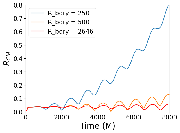
Figure 8: The drift of the coordinate center of mass in BBH simulations using the freezing-$\Psi_{0}$ boundary condition at $R_{\rm bdry}=250M$, $500M$, and $2,646M$.

Further examination of the $\Phi^{+}_{2,2}$ error reveals that the early-time error for $L=1$ is much lower when the test $R_{\rm bdry}=500M$ than it is when $R_{\rm bdry}=250M$. Consequently, the difference in early-time error between $L=1$ and $L=4$ is smaller when $R_{\rm bdry}=500M$. For the modes $\Phi^{-}_{2,1}$ and $\Phi^{+}_{3,1}$, the fourth order method gives reduced errors for the duration of the simulation for both boundary locations, even though it grows after $t\approx 4,500$. This growth in error, which occurs in most of the tests plotted, could be the result of compounding errors accumulating from outer boundary reflections and/or gauge BC errors.

Finally, let us consider the $\Phi^{+}_{2,0}$ mode more thoroughly. This mode should contain the largest contribution to GW memory effects and has been difficult to compute in numerical relativity simulations Favata (2009) without Cauchy characteristic extraction Mitman et al. (2020) or post-processing Mitman et al. (2021) methods. In Figures 6 and 7, the $\Phi^{+}_{2,0}$ mode error settles to a value offset from zero with the standard $L=1$ freezing-$\Psi_{0}$ boundary condition. With the $L=4$ WeylHOBC method, however, the error in $\Phi^{+}_{2,0}$ quickly settles to zero, although if $\text{w}_{k\ell m}^{(\pm)}$ are incorrectly initialized to zero, the error has a large initial transient. These results indicate that HOBC with $L=4$ gives more accurate results for $\Phi^{+}_{2,0}$ than does the freezing-$\Psi_{0}$ boundary condition, with respect to the reference run. Conclusions cannot be made about the accuracy of the memory effects, however, without further analysis Mitman et al. (2020).

The appearance of a small amount of high-frequency noise in the errors of all modes at early times in Figure 7 warrants explanation. Notice that this noise disappears rather abruptly at $t\approx 4,800M$. This high-frequency component is present only in the reference run and thus shows up in the difference between waves extracted from the $R_{\rm bdry}=500M$ runs and the reference run. Its presence in the reference run is due to high-frequency, short-wavelength junk radiation in the initial data which pervades the grid. It persists in the reference run for about the amount of time a signal takes to pass from near the binary black holes to the reference outer boundary of $R=2,646M$ and back again to $R_{\rm bdry}=500M$ (which would be a total time of $4,792M$). One might have hoped that the $L=4$ WeylHOBC in the reference run would have eliminated even a single round of reflections, but this short-wavelength radiation is not well resolved by the SpEC code at the grid resolutions we have used, so unphysical backscatter and reflections are possible even with absorbing boundary conditions. This high frequency junk radiation component is not visible in Figure 6 (which shows the $R_{\rm bdry}=250M$ boundary errors) because these errors are larger; hence, the scales of the plots are larger.

In Figure 9, we study the convergence of our runs with numerical resolution. We plot the differences between consecutively higher resolutions for the $R_{\rm bdry}=500M$ runs using 4th order WeylHOBCs with properly initialized $\text{w}_{k\ell m}^{(\pm)}$. Here “Lev” in the figure refers to the adaptive-mesh-refinement tolerance that determines the grid resolution; larger Levs have finer grids. All the modes show nice convergence except for the $\Phi^{+}_{2,0}$ mode in the time range $3,000M<t<4,000M$. We attribute the non-convergence in this time range to the fact that $\Phi^{+}_{2,0}$ is primarily non-oscillatory, in the sense that there is a non-zero offset component to the wave, which dwarfs the sinusoid, and in addition there is a linear drift component. Because of these features, when the amplitude of the $\Phi^{+}_{2,0}$ mode with one resolution crosses the amplitude of the same mode with a different resolution at $t\approx 3,000M$, they linger close to each other. On the other hand, the other modes, which show nice convergence properties, are more purely oscillatory. Thus, zero crossings between resolutions are sharp and brief, as seen in the remaining five panels of Figure 9.

Figure 9: Convergence plots for BBH simulations using $L=4$ WeylHOBC and proper $\text{w}_{k\ell m}$ initialization. Test $R_{\rm bdry}=500M$, reference $R_{\rm bdry}=2,646M$, and all waves are extracted at $R_{\rm bdry}=500M$. Branching into different resolutions (Levs) is done after junk radiation from the initial data has left the grid, so all resolutions are identical up to $t=1,500M$. Convergence plots for the other cases (runs with $L=4$ WeylHOBC but no proper $\text{w}_{k\ell m}$ initialization, those using the freezing-$\Psi_{0}$ boundary condition, and reference runs) all show similar results.

Finally, there is no extra computational cost when implementing the HOBCs for BBH simulations. HOBC runs are found to run at about the same speed as those using SpEC’s freezing-$\Psi_{0}$ boundary condition.

V Conclusions and Future Work

We have presented two new implementations of the high-order absorbing boundary conditions for the Einstein field equations, WeylHOBC and dtHOBC, and find WeylHOBC to be clearly superior in accuracy, robustness, and simplicity of implementation (given a code that already uses the freezing-$\Psi_{0}$ boundary condition). Our findings may also be applicable to other schemes that involve coupling an interior evolution to an auxiliary system, such as Cauchy characteristic matching. Considered in itself, the WeylHOBC method has proven stable in binary black hole simulations and has shown that it can produce higher accuracy at a given boundary location than the freezing-$\Psi_{0}$ condition, especially for the subdominant modes and for the $(2,0)$ mode which contains GW memory effects. We have also demonstrated a simple recipe for initializing the $\text{w}_{k\ell m}^{(\pm)}$ auxiliary functions, which significantly reduces initial transients. This recipe is the first attempt to satisfy compatibility conditions between the initial and boundary surfaces.

Although successful implementation of WeylHOBCs for BBHs has been demonstrated, there are several avenues for future work to gain increased accuracy in the years ahead. Implementation of the first order corrections for curvature and backscatter given in Buchman and Sarbach (2007) would improve accuracy even further and allow for smaller computational grids. By simulating BBHs through merger and ringdown, one could perhaps reproduce correctly the tail decay. Implementing WeylHOBCs without demanding the outer boundary radius to be constant in time would perhaps further increase accuracy by allowing various outgoing characteristic fields to exit the grid as the evolution proceeds. Finally, we plan to compare the accuracy of gravitational waveforms computed with our WeylHOBCs to those computed with the recent implementation of CCM in the SpECTRE code.

The center of mass drift problem seen in SXS long-time BBH simulations was not improved by our WeylHOBCs, leading one to believe that the source of this problem is from the gauge boundary conditions. We plan to investigate whether or not some form of WeylHOBCs could be applied to the gauge modes and thereby alleviate this problem.

VI Acknowledgements

It is a pleasure to thank Olivier Sarbach for providing comments on the paper prior to publication, for many consultations, and for hosting L.T.B. at the 2019 BIRS-CMO workshop in Oaxaca, Mexico. Additionally, we thank Joey Key for her support at UW Bothell, and Dante Iozzo, Stephen Lau, and Oscar Reula for their insights and suggestions. Finally, L.T.B. dedicates this paper to the memory of James M. Bardeen, mentor and friend.

M.D. gratefully acknowledges support from the NSF through grant PHY-2110287 and from NASA through grant 80NSSC22K0719. M.M. gratefully acknowledges support from the NSF through grant AST-2219109 and to the DOE through a Computational Science Graduate Fellowship. This material is based upon work supported by the U.S. Department of Energy, Office of Science, Office of Advanced Scientific Computing Research under Award Number DE-SC0024386. M.S. gratefully acknowledges support from the Sherman Fairchild Foundation and from NSF grants PHY-2309211, PHY-2309231, and OAC-2209656. T.M.K. and A.E. were supported by NSF Physics REU Award 2050928 and T.M.K. was also supported by NSF CAREER Award 1944412.

This report was prepared as an account of work sponsored by an agency of the United States Government. Neither the United States Government nor any agency thereof, nor any of their employees, makes any warranty, express or implied, or assumes any legal liability or responsibility for the accuracy, completeness, or usefulness of any information, apparatus, product, or process disclosed, or represents that its use would not infringe privately owned rights. Reference herein to any specific commercial product, process, or service by trade name, trademark, manufacturer, or otherwise does not necessarily constitute or imply its endorsement, recommendation, or favoring by the United States Government or any agency thereof. The views and opinions of authors expressed herein do not necessarily state or reflect those of the United States Government or any agency thereof.

References

- Buchman and Sarbach (2006) L. T. Buchman and O. C. A. Sarbach, Classical and Quantum Gravity 23, 6709 (2006).
- Aasi et al. (2015) J. Aasi et al. (LIGO Scientific Collaboration), Class. Quantum Grav. 32, 074001 (2015).
- Acernese et al. (2015) F. Acernese et al. (Virgo Collaboration), Class. Quantum Grav. 32, 024001 (2015).
- Akutsu et al. (2021) T. Akutsu et al. (KAGRA Collaboration), Prog. Theor. Exp. Phys. 2021, 05A101 (2021).
- Amaro-Seoane et al. (2023) P. Amaro-Seoane, J. Andrews, M. Arca Sedda, et al., Living Rev. Relativity 26 (2023), cited November 2023, URL https://doi.org/10.1007/s41114-022-00041-y.
- Afshordi et al. (2023) N. Afshordi et al. (LISA Consortium Waveform Working Group) (2023), eprint 2311.01300.
- Ferguson et al. (2021) D. Ferguson, K. Jani, P. Laguna, and D. Shoemaker, Phys. Rev. D 104, 044037 (2021).
- Pürrer and Haster (2020) M. Pürrer and C.-J. Haster, Phys. Rev. Res. 2, 023151 (2020).
- Mehta et al. (2023) A. K. Mehta, S. Olsen, D. Wadekar, J. Roulet, T. Venumadhav, J. Mushkin, B. Zackay, and M. Zaldarriaga (2023), eprint 2311.06061.
- Cotesta et al. (2018) R. Cotesta, A. Buonanno, A. Bohé, A. Taracchini, I. Hinder, and S. Ossokine, Phys. Rev. D 98, 084028 (2018).
- et al. (LIGO Scientific Collaboration and Collaboration) R. A. et al. (LIGO Scientific Collaboration and V. Collaboration), Phys. Rev. D 102, 043015 (2020).
- Shaik et al. (2020) F. H. Shaik, J. Lange, S. E. Field, R. O’Shaughnessy, V. Varma, L. E. Kidder, H. P. Pfeiffer, and D. Wysocki, Phys. Rev. D 101, 124054 (2020).
- Yang et al. (2023) T. Yang, R.-G. Cai, Z. Cao, and H. M. Lee (2023), eprint 2310.08160.
- Favata (2009) M. Favata, Phys. Rev. D 80, 024002 (2009).
- Mitman et al. (2020) K. Mitman, J. Moxon, M. A. Scheel, S. A. Teukolsky, M. Boyle, N. Deppe, L. E. Kidder, and W. Throwe, Phys. Rev. D 102, 104007 (2020).
- Joshi et al. (2023) A. V. Joshi, S. G. Rosofsky, R. Haas, and E. A. Huerta, Phys. Rev. D 107, 064038 (2023).
- Mills and Fairhurst (2021) C. Mills and S. Fairhurst, Phys. Rev. D 103, 024042 (2021).
- Chandra et al. (2022) K. Chandra, J. Calderón Bustillo, A. Pai, and I. W. Harry, Phys. Rev. D 106, 123003 (2022).
- Islam et al. (2021) T. Islam, S. E. Field, C.-J. Haster, and R. Smith, Phys. Rev. D 103, 104027 (2021).
- Colleoni et al. (2021) M. Colleoni, M. Mateu-Lucena, H. Estellés, C. García-Quirós, D. Keitel, G. Pratten, A. Ramos-Buades, and S. Husa, Phys. Rev. D 103, 024029 (2021).
- Buchman et al. (2012) L. T. Buchman, H. P. Pfeiffer, M. A. Scheel, and B. Szilágyi, Phys. Rev. D 86, 084033 (2012).
- Sarbach and Tiglio (2012) O. Sarbach and M. Tiglio, Living Rev. Relativity 15, 9 (2012), cited August 2021, URL http://www.livingreviews.org/lrr-2012-9.
- Buchman and Sarbach (2007) L. T. Buchman and O. C. A. Sarbach, Classical and Quantum Gravity 24, S307 (2007).
- (24) L. Kidder, H. Pfeifer, and M. Scheel, Spectral einstein code, URL https://www.black-holes.org/code/SpEC.html.
- Ruiz et al. (2007) M. Ruiz, O. Rinne, and O. Sarbach, Classical and Quantum Gravity 24, 6349 (2007).
- Kreiss and Winicour (2006) H. O. Kreiss and J. Winicour, Classical and Quantum Gravity 23, S405 (2006).
- Kreiss et al. (2007) H.-O. Kreiss, O. A. Reula, O. Sarbach, and J. Winicour, Classical and Quantum Gravity 24, 5973 (2007).
- Rinne et al. (2009) O. Rinne, L. T. Buchman, M. A. Scheel, and H. P. Pfeiffer, Class. Quantum Grav. 26, 075009 (2009).
- Lindblom et al. (2006) L. Lindblom, M. A. Scheel, L. E. Kidder, R. Owen, and O. Rinne, Class. Quant. Grav. 23, S447 (2006).
- Regge and Wheeler (1957) T. Regge and J. A. Wheeler, Phys. Rev. 108, 1063 (1957).
- Zerilli (1970) F. J. Zerilli, Phys. Rev. Lett. 24, 737 (1970).
- Rinne (2009) O. Rinne, Class. Quantum Grav. 26, 048003 (2009).
- Scheel et al. (2006) M. A. Scheel, H. P. Pfeiffer, L. Lindblom, L. E. Kidder, O. Rinne, and S. A. Teukolsky, Physical Review D 74, 104006 (2006).
- Rauch and Massey (1974) J. B. Rauch and F. J. Massey, Transactions of the American Mathematical Society 189, 303 (1974).
- Winicour (2012) J. Winicour, Living Rev. Relativity 15 (2012), URL https://doi.org/10.12942/lrr-2012-2.
- Bishop et al. (1999) N. T. Bishop, R. Gomez, L. Lehner, B. Szilágyi, J. Winicour, and R. A. Isaacson, in Black Holes, Gravitational Radiation and the Universe: Essays in Honor of C.V. Vishveshwara, edited by B. R. Iyer and B. Bhawal (Springer Netherlands, Dordrecht, 1999), pp. 383–408.
- Szilágyi (2000) B. Szilágyi, Cauchy-characteristic matching in general relativity (2000), eprint gr-qc/0006091.
- Calabrese (2006) G. Calabrese, Classical and Quantum Gravity 23, 5439–5450 (2006).
- Ma et al. (2023) S. Ma, J. Moxon, M. A. Scheel, K. C. Nelli, N. Deppe, M. S. Bonilla, L. E. Kidder, P. Kumar, G. Lovelace, W. Throwe, et al. (2023), eprint gr-qc/2308.10361.
- York (1979) J. York, J. W., in Sources of Gravitational Radiation, edited by L. L. Smarr (1979), pp. 83–126.
- Bondi et al. (1962) H. Bondi, M. G. J. van der Burg, and A. W. K. Metzner, Proc. R. Soc. Lond. A 269, 21 (1962).
- Sachs (1962) R. K. Sachs, Proc. R. Soc. of Lond. A 270, 103 (1962).
- Stewart (1989) J. M. Stewart, Proc. R. Soc. Lond. A 424, 211 (1989).
- Deppe, Nils and Throwe, William and Kidder, Lawrence E. and Vu, Nils L. and others (2023) Deppe, Nils and Throwe, William and Kidder, Lawrence E. and Vu, Nils L. and others, SpECTRE (2023), v. 2023.10.11, URL https://doi.org/10.5281/zenodo.8431874.
- Giannakopoulos et al. (2020) T. Giannakopoulos, D. Hilditch, and M. Zilhão, Phys. Rev. D 102, 064035 (2020).
- Giannakopoulos et al. (2023) T. Giannakopoulos, N. T. Bishop, D. Hilditch, D. Pollney, and M. Zilhão, Phys. Rev. D 108, 104033 (2023).
- Sarbach and Tiglio (2001) O. Sarbach and M. Tiglio, Phys. Rev. D 64, 084016 (2001).
- Bayliss and Turkel (1980) A. Bayliss and E. Turkel, Comm. Pure Appl. Math. 33, 707 (1980).
- Boyle et al. (2019) M. Boyle et al., Class. Quant. Grav. 36, 195006 (2019).
- Kidder et al. (2005) L. E. Kidder, L. Lindblom, M. A. Scheel, L. T. Buchman, and H. P. Pfeiffer, Phys. Rev. D 71, 064020 (2005).
- Bjørhus (1995) M. Bjørhus, SIAM Journal on Scientific Computing 16, 542 (1995).
- Bardeen and Buchman (2002) J. M. Bardeen and L. T. Buchman, Physical Review D 65, 064037 (2002).
- Reula and Sarbach (2005) O. Reula and O. Sarbach, J. Hyperbol. Diff. Equat. 2, 397 (2005).
- Teukolsky (1982) S. A. Teukolsky, Phys. Rev. D 26, 745 (1982).
- Lovelace et al. (2008) G. Lovelace, R. Owen, H. P. Pfeiffer, and T. Chu, Physical Review D 78, 084017 (2008).
- Szilágyi et al. (2015) B. Szilágyi, J. Blackman, A. Buonanno, A. Taracchini, H. P. Pfeiffer, M. A. Scheel, T. Chu, L. E. Kidder, and Y. Pan, Physical Review Letters 115, 031102 (2015).
- Boyle (2016) M. Boyle, Physical Review D 93, 084031 (2016).
- (58) D. Sun, in progress.
- Mitman et al. (2021) K. Mitman, D. A. B. Iozzo, N. Khera, M. Boyle, T. De Lorenzo, N. Deppe, L. E. Kidder, J. Moxon, H. P. Pfeiffer, M. A. Scheel, et al., Phys. Rev. D 103, 024031 (2021).