FiT: Flexible Vision Transformer for Diffusion Model

Abstract

Nature is infinitely resolution-free. In the context of this reality, existing diffusion models, such as Diffusion Transformers, often face challenges when processing image resolutions outside of their trained domain. To overcome this limitation, we present the Flexible Vision Transformer (FiT), a transformer architecture specifically designed for generating images with unrestricted resolutions and aspect ratios. Unlike traditional methods that perceive images as static-resolution grids, FiT conceptualizes images as sequences of dynamically-sized tokens. This perspective enables a flexible training strategy that effortlessly adapts to diverse aspect ratios during both training and inference phases, thus promoting resolution generalization and eliminating biases induced by image cropping. Enhanced by a meticulously adjusted network structure and the integration of training-free extrapolation techniques, FiT exhibits remarkable flexibility in resolution extrapolation generation. Comprehensive experiments demonstrate the exceptional performance of FiT across a broad range of resolutions, showcasing its effectiveness both within and beyond its training resolution distribution. Repository available at https://github.com/whlzy/FiT.

1 Introduction

Current image generation models struggle with generalizing across arbitrary resolutions. The Diffusion Transformer (DiT) (Peebles & Xie, 2023) family, while excelling within certain resolution ranges, falls short when dealing with images of varying resolutions. This limitation stems from the fact that DiT can not utilize dynamic resolution images during its training process, hindering its ability to adapt to different token lengths or resolutions effectively.

To overcome this limitation, we introduce the Flexible Vision Transformer (FiT), which is adept at generating images at unrestricted resolutions and aspect ratios. The key motivation is a novel perspective on image data modeling: rather than treating images as static grids of fixed dimensions, FiT conceptualizes images as sequences of variable-length tokens. This approach allows FiT to dynamically adjust the sequence length, thereby facilitating the generation of images at any desired resolution without being constrained by pre-defined dimensions. By efficiently managing variable-length token sequences and padding them to a maximum specified length, FiT unlocks the potential for resolution-independent image generation. FiT represents this paradigm shift through significant advancements in flexible training pipeline, network architecture, and inference processes.

Flexible Training Pipeline. FiT uniquely preserves the original image aspect ratio during training, by viewing the image as a sequence of tokens. This unique perspective allows FiT to adaptively resize high-resolution images to fit within a predefined maximum token limit, ensuring that no image, regardless of its original resolution, is cropped or disproportionately scaled. This method ensures that the integrity of the image resolution is maintained, as shown in Figure 2, facilitating the ability to generate high-fidelity images at various resolutions. To the best of our knowledge, FiT is the first transformer-based generation model to maintain diverse image resolutions throughout training.

Network Architecture. The FiT model evolves from the DiT architecture but addresses its limitations in resolution extrapolation. One essential network architecture adjustment to handle diverse image sizes is the adoption of 2D Rotary Positional Embedding (RoPE) (Su et al., 2024), inspired by its success in enhancing large language models (LLMs) for length extrapolation (Liu et al., 2023). We also introduce Swish-Gated Linear Unit (SwiGLU) (Shazeer, 2020) in place of the traditional Multilayer Perceptron (MLP) and replace DiT’s Multi-Head Self-Attention (MHSA) with Masked MHSA to efficiently manage padding tokens within our flexible training pipeline.

Inference Process. While large language models employ token length extrapolation techniques (Peng et al., 2023; LocalLLaMA, ) for generating text of arbitrary lengths, a direct application of these technologies to FiT yields suboptimal results. We tailor these techniques for 2D RoPE, thereby enhancing FiT’s performance across a spectrum of resolutions and aspect ratios.

Our highest Gflop FiT-XL/2 model, after training for only 1.8 million steps on ImageNet-256 (Deng et al., 2009) dataset, outperforms all state-of-the-art CNN and transformer models by a significant margin across resolutions of $160\times 320$, $128\times 384$, $320\times 320$, $224\times 448$, and $160\times 480$. The performance of FiT-XL/2 significantly advances further with our training-free resolution extrapolation method. Compared to the baseline DiT-XL/2 training for 7 million steps, FiT-XL/2 lags slightly at the resolution of $256\times 256$ but significantly surpasses it at all other resolutions.

In summary, our contributions lie in the novel introduction of FiT, a flexible vision transformer tailored for diffusion models, capable of generating images at any resolution and aspect ratio. We present three innovative design features in FiT, including a flexible training pipeline that eliminates the need for cropping, a unique transformer architecture for dynamic token length modeling, and a training-free resolution extrapolation method for arbitrary resolution generation. Strict experiments demonstrate that the FiT-XL/2 model achieves state-of-the-art performance across a variety of resolution and aspect ratio settings.

Figure 2: Pipeline comparison between (a) DiT and (b) FiT.

2 Related Work

Diffusion Models. Denoising Diffusion Probabilistic Models (DDPMs) (Ho et al., 2020; Saharia et al., 2022; Radford et al., 2021) and score-based models (Hyvärinen & Dayan, 2005; Song et al., 2020b) have exhibited remarkable progress in the context of image generation tasks. The Denoising Diffusion Implicit Model (DDIM) Song et al. (2020a), offers An accelerated sampling procedure. Latent Diffusion Models (LDMs) (Rombach et al., 2022) establishes a new benchmark of training deep generative models to reverse a noise process in the latent space, through the use of VQ-VAE (Esser et al., 2021).

Transformer Models. The Transformer model (Vaswani et al., 2017), has successfully supplanted domain-specific architectures in a variety of fields including, but not limited to, language (Brown et al., 2020; Chowdhery et al., 2023a), vision (Dosovitskiy et al., 2020), and multi-modality (Team et al., 2023). In vision perception research, most efforts (Touvron et al., 2019, 2021; Liu et al., 2021, 2022) that focus on resolution are aimed at accelerating pretraining using a fixed, low resolution. On the other hand, NaViT (Dehghani et al., 2023) implements the ’Patch n’ Pack’ technique to train ViT using images at their natural, ’native’ resolution. Notably, transformers have been also explored in the denoising diffusion probabilistic models (Ho et al., 2020) to synthesize images. DiT (Peebles & Xie, 2023) is the seminal work that utilizes a vision transformer as the backbone of LDMs and can serve as a strong baseline. Based on DiT architecture, MDT (Gao et al., 2023) introduces a masked latent modeling approach, which requires two forward-runs in training and inference. U-ViT (Bao et al., 2023) treats all inputs as tokens and incorporates U-Net architectures into the ViT backbone of LDMs. DiffiT (Hatamizadeh et al., 2023) introduces a time-dependent self-attention module into the DiT backbone to adapt to different stages of the diffusion process. We follow the LDM paradigm of the above methods and further propose a novel flexible image synthesis pipeline.

Length Extrapolation in LLMs. RoPE (Rotary Position Embedding) (Su et al., 2024) is a novel positional embedding that incorporates relative position information into absolute positional embedding. It has recently become the dominant positional embedding in a wide range of LLM (Large Language Model) designs (Chowdhery et al., 2023b; Touvron et al., 2023a, b). Although RoPE enjoys valuable properties, such as the flexibility of sequence length, its performance drops when the input sequence surpasses the training length. Many approaches have been proposed to solve this issue. PI (Position Interpolation) (Chen et al., 2023) linearly down-scales the input position indices to match the original context window size, while NTK-aware (LocalLLaMA, ) changes the rotary base of RoPE. YaRN (Yet another RoPE extensioN) (Peng et al., 2023) is an improved method to efficiently extend the context window. RandomPE (Ruoss et al., 2023) sub-samples an ordered set of positions from a much larger range of positions than originally observed in training or inference. xPos (Sun et al., 2022) incorporates long-term decay into RoPE and uses blockwise causal attention for better extrapolation performance. Our work delves deeply into the implementation of RoPE in vision generation and on-the-fly resolution extrapolation methods.

3 Flexible Vision Transformer for Diffusion

Figure 3: Overview of (a) flexible training pipeline, (b) flexible inference pipeline, and (c) FiT block.

3.1 Preliminary

1-D RoPE (Rotary Positional Embedding) (Su et al., 2024) is a type of position embedding that unifies absolute and relative PE, exhibiting a certain degree of extrapolation capability in LLMs. Given the m-th key and n-th query vector as $\mathbf{q}_{m},\mathbf{k}_{n}\in\mathbb{R}^{|D|}$, 1-D RoPE multiplies the bias to the key or query vector in the complex vector space:

$$f_{q}(\mathbf{q}_{m},m)=e^{im\Theta}\mathbf{q}_{m},\quad f_{k}(\mathbf{k}_{n},n)=e^{in\Theta}\mathbf{k}_{n}$$ (1)

where $\Theta=\mathrm{Diag}(\theta_{1},\cdots,\theta_{|D|/2})$ is rotary frequency matrix with $\theta_{d}=b^{-2d/|D|}$ and rotary base $b=10000$. In real space, given $l=|D|/2$, the rotary matrix $e^{im\Theta}$ equals to:

$$\begin{bmatrix}\cos m\theta_{1}&-\sin m\theta_{1}&\cdots&0&0\\ \sin m\theta_{1}&\cos m\theta_{1}&\cdots&0&0\\ \vdots&\vdots&\ddots&\vdots&\vdots\\ 0&0&\cdots&\cos m\theta_{l}&-\sin m\theta_{l}\\ 0&0&\cdots&\sin m\theta_{l}&\cos m\theta_{l}\end{bmatrix}$$ (2)

The attention score with 1-D RoPE is calculated as:

$$A_{n}=\mathrm{Re}\langle f_{q}(\mathbf{q}_{m},m),f_{k}(\mathbf{k}_{n},n)\rangle$$ (3)

NTK-aware Interpolation (LocalLLaMA, ) is a training-free length extrapolation technique in LLMs. To handle the larger context length $L_{\text{test}}$ than maximum training length $L_{\text{train}}$, it modifies the rotary base of 1-D RoPE as follows:

$$b^{\prime}=b\cdot s^{\frac{|D|}{|D|-2}},$$ (4)

where the scale factor $s$ is defined as:

$$s=\max(\frac{L_{test}}{L_{train}},1.0).$$ (5)

YaRN (Yet another RoPE extensioN) Interpolation (Peng et al., 2023) introduces the ratio of dimension $d$ as $r(d)={L_{\text{train}}}/({2\pi b^{2d/|D|}})$, and modifies the rotary frequency as:

$$\theta^{\prime}_{d}=\left(1-\gamma(r(d))\right)\frac{\theta_{d}}{s}+\gamma(r(d))\theta_{d},$$ (6)

where $s$ is the aforementioned scale factor, and $\gamma(r(d))$ is a ramp function with extra hyper-parameters $\alpha,\beta$:

$$\gamma(r)=\begin{cases}0,&\text{if }r<\alpha\\ 1,&\text{if }r>\beta\\ \frac{r-\alpha}{\beta-\alpha},&\text{otherwise}.\end{cases}$$ (7)

Besides, it incorporates a 1D-RoPE scaling term as:

$$f^{\prime}_{q}(\mathbf{q}_{m},m)=\frac{1}{\sqrt{t}}f_{q}(\mathbf{q}_{m},m),f^{\prime}_{k}(\mathbf{k}_{n},n)=\frac{1}{\sqrt{t}}f_{k}(\mathbf{k}_{n},n),$$ (8)

where $\frac{1}{\sqrt{t}}=0.1\ln(s)+1$.

3.2 Flexible Training and Inference Pipeline

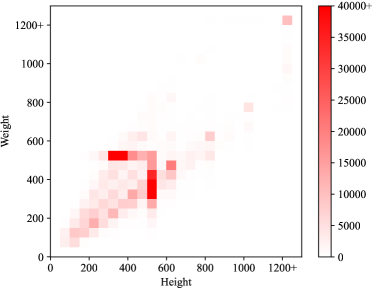
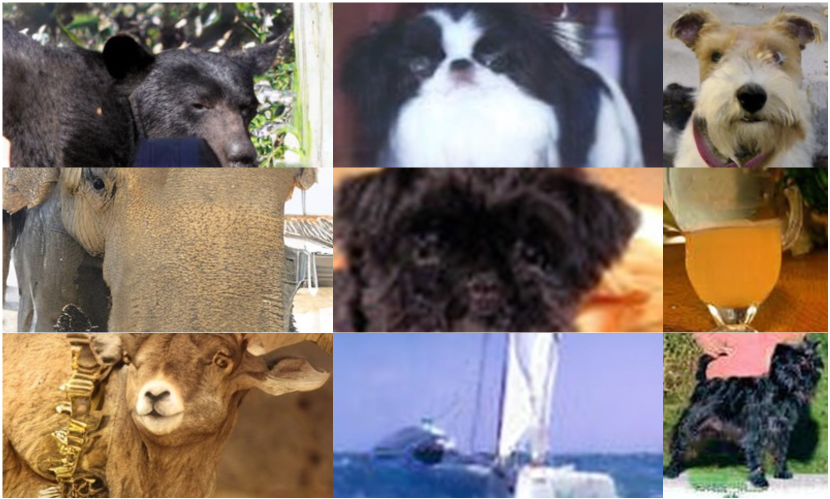
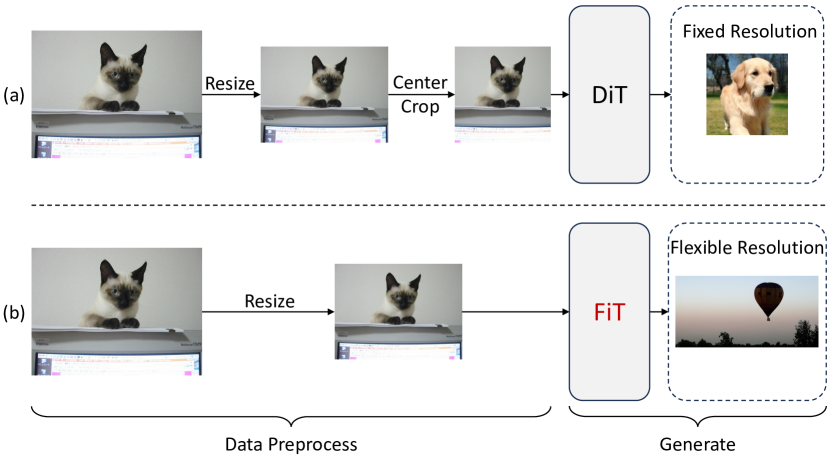
Modern deep learning models, constrained by the characteristics of GPU hardware, are required to pack data into batches of uniform shape for parallel processing. Due to the diversity in image resolutions, as shown in Fig. 4, DiT resizes and crops the images to a fixed resolution $256\times 256$. While resizing and cropping as a means of data augmentation is a common practice, this approach introduces certain biases into the input data. These biases will directly affect the final images generated by the model, including blurring effects from the transition from low to high resolution and information lost due to the cropping (more failure samples can be found in Appendix  D).

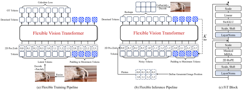
To this end, we propose a flexible training and inference pipeline, as shown in Fig. 3 (a, b). In the preprocessing phase, we avoid cropping images or resizing low-resolution images to a higher resolution. Instead, we only resize high-resolution images to a predetermined maximum resolution limit, $HW\leqslant 256^{2}$. In the training phase, FiT first encodes an image into latent codes with a pre-trained VAE encoder. By patchfiying latent codes to latent tokens, we can get sequences with different lengths $L$. To pack these sequences into a batch, we pad all these sequences to the maximum token length $L_{max}$ using padding tokens. Here we set $L_{max}=256$ to match the fixed token length of DiT. The same as the latent tokens, we also pad the positional embeddings to the maximum length for packing. Finally, we calculate the loss function only for the denoised output tokens, while discarding all other padding tokens. In the inference phase, we firstly define the position map of the generated image and sample noisy tokens from the Gaussian distribution as input. After completing $K$ iterations of the denoising process, we reshape and unpatchfiy the denoised tokens according to the predefined position map to get the final generated image.

3.3 Flexible Vision Transformer Architecture

Building upon the flexible training pipeline, our goal is to find an architecture that can stably train across various resolutions and generate images with arbitrary resolutions and aspect ratios, as shown in Figure 3 (c). Motivated by some significant architectural advances in LLMs, we conduct a series of experiments to explore architectural modifications based on DiT, see details in Section 4.2.

Replacing MHSA with Masked MHSA. The flexible training pipeline introduces padding tokens for flexibly packing dynamic sequences into a batch. During the forward phase of the transformer, it is crucial to facilitate interactions among noised tokens while preventing any interaction between noised tokens and padding tokens. The Multi-Head Self-Attention (MHSA) mechanism of original DiT is incapable of distinguishing between noised tokens and padding tokens. To this end, we use Masked MHSA to replace the standard MHSA. We utilize the sequence mask $M$ for Masked Attention, where noised tokens are assigned the value of $0$, and padding tokens are assigned the value of negative infinity (-inf), which is defined as follows:

$$\text{Masked Attn.}(Q_{i},K_{i},V_{i})=\text{Softmax}\left(\frac{Q_{i}K_{i}^{T}}{\sqrt{d_{k}}}+M\right)V_{i}$$ (9)

where $Q_{i}$, $K_{i}$, $V_{i}$ are the query, key, and value matrices for the $i$-th head.

Replacing Absolute PE with 2D RoPE. We observe that vision transformer models with absolute positional embedding fail to generalize well on images beyond the training resolution, as in Sections 4.3 and 4.5. Inspired by the success of 1D-RoPE in LLMs for length extrapolation (Liu et al., 2023), we utilize 2D-RoPE to facilitate the resolution generalization in vision transformer models. Formally, we calculate the 1-D RoPE for the coordinates of height and width separately. Then such two 1-D RoPEs are concatenated in the last dimension. Given 2-D coordinates of width and height as $\{(w,h)\Big{|}1\leqslant w\leqslant W,1\leqslant h\leqslant H\}$, the 2-D RoPE is defined as:

$$f_{q}(\mathbf{q}_{m},h_{m},w_{m})=[e^{ih_{m}\Theta}\mathbf{q}_{m}\parallel e^{iw_{m}\Theta}\mathbf{q}_{m}],$$ (10)

$$f_{k}(\mathbf{k}_{n},h_{n},w_{n})=[e^{ih_{n}\Theta}\mathbf{k}_{n}\parallel e^{iw_{n}\Theta}\mathbf{k}_{n}],$$

where $\Theta=\mathrm{Diag}(\theta_{1},\cdots,\theta_{|D|/4})$, and $\parallel$ denotes concatenate two vectors in the last dimension. Note that we divide the $|D|$-dimension space into $|D|/4$-dimension subspace to ensure the consistency of dimension, which differs from $|D|/2$-dimension subspace in 1-D RoPE. Analogously, the attention score with 2-D RoPE is:

$$A_{n}=\mathrm{Re}\langle f_{q}(\mathbf{q}_{m},h_{m},w_{m}),f_{k}(\mathbf{k}_{n},h_{n},w_{n})\rangle.$$ (11)

It is noteworthy that there is no cross-term between $h$ and $w$ in 2D-RoPE and attention score $A_{n}$, so we can further decouple the rotary frequency as $\Theta_{h}$ and $\Theta_{w}$, resulting in the decoupled 2D-RoPE, which will be discussed in Section 3.4 and more details can be found in Appendix  B.

Replacing MLP with SwiGLU. We follow recent LLMs like LLaMA (Touvron et al., 2023a, b), and replace the MLP in FFN with SwiGLU, which is defined as follows:

$$\begin{split}\text{SwiGLU}(x,W,V)=\text{SiLU}(xW)\otimes(xV)\\ \text{FFN}(x)=\text{SwiGLU}(x,W_{1},W_{2})W_{3}\end{split}$$ (12)

where $\otimes$ denotes Hadmard Product, $W_{1}$, $W_{2}$, and $W_{3}$ are the weight matrices without bias, $\text{SiLU}(x)=x\otimes\sigma(x)$. Here we will use SwiGLU as our choice in each FFN block.

3.4 Training Free Resolution Extrapolation

We denote the inference resolution as ($H_{\text{test}}$, $W_{\text{test}}$). Our FiT can handle various resolutions and aspect ratios during training, so we denote training resolution as $L_{\text{train}}=\sqrt{L_{\text{max}}}$.

By changing the scale factor in Equation 5 to $s=\max({\max(H_{\text{test}},W_{\text{test}})}/{L_{train}},1.0)$, we can directly implement the positional interpolation methods in large language model extrapolation on 2D-RoPE, which we call vanilla NTK and YaRN implementation. Furthermore, we propose vision RoPE interpolation methods by using the decoupling attribute in decoupled 2D-RoPE. We modify Equation 10 to:

$$\hat{f}_{q}(\mathbf{q}_{m},h_{m},w_{m})=[e^{ih_{m}\Theta_{h}}\mathbf{q}_{m}\parallel e^{iw_{m}\Theta_{w}}\mathbf{q}_{m}],$$ (13)

$$\hat{f}_{k}(\mathbf{k}_{n},h_{n},w_{n})=[e^{ih_{n}\Theta_{h}}\mathbf{k}_{n}\parallel e^{iw_{n}\Theta_{w}}\mathbf{k}_{n}],$$

where $\Theta_{h}=\{\theta^{h}_{d}=b_{h}^{-2d/|D|},1\leqslant d\leqslant\frac{|D|}{2}\}$ and $\Theta_{w}=\{\theta^{w}_{d}=b_{w}^{-2d/|D|},1\leqslant d\leqslant\frac{|D|}{2}\}$ are calculated separately. Accordingly, the scale factor of height and width is defined separately as

$$s_{h}=\max(\frac{H_{\text{test}}}{L_{\text{train}}},1.0),\quad s_{w}=\max(\frac{W_{\text{test}}}{L_{\text{train}}},1.0).$$ (14)

Definition 3.1.

The Definition of VisionNTK Interpolation is a modification of NTK-aware Interpolation by using Equation 13 with the following rotary base.

$$b_{h}=b\cdot s_{h}^{\frac{|D|}{|D|-2}},\quad b_{w}=b\cdot s_{w}^{\frac{|D|}{|D|-2}},$$ (15)

where $b=10000$ is the same with Equation 1

Definition 3.2.

The Definition of VisionYaRN Interpolation is a modification of YaRN Interpolation by using Equation 13 with the following rotary frequency.

$$\theta^{h}_{d}=(1-\gamma(r(d))\frac{\theta_{d}}{s_{h}}+\gamma(r(d))\theta_{d},$$ (16)

$$\theta^{w}_{d}=(1-\gamma(r(d))\frac{\theta_{d}}{s_{w}}+\gamma(r(d))\theta_{d},$$

where $\gamma(r(d))$ is the same with Equation 6.

It is worth noting that VisionNTK and VisionYaRN are training-free positional embedding interpolation approaches, used to alleviate the problem of position embedding out of distribution in extrapolation. When the aspect ratio equals one, they are equivalent to the vanilla implementation of NTK and YaRN. They are especially effective in generating images with arbitrary aspect ratios, see Section 4.3.

4 Experiments

Method Train Cost 256$\times$256 (1:1) 160$\times$320 (1:2) 128$\times$384 (1:3) FID$\downarrow$ sFID$\downarrow$ IS$\uparrow$ Prec.$\uparrow$ Rec.$\uparrow$ FID$\downarrow$ sFID$\downarrow$ IS$\uparrow$ Prec.$\uparrow$ Rec.$\uparrow$ FID$\downarrow$ sFID$\downarrow$ IS$\uparrow$ Prec.$\uparrow$ Rec.$\uparrow$ BigGAN-deep - 6.95 7.36 171.4 0.87 0.28 - - - - - - - - - - StyleGAN-XL - 2.30 4.02 265.12 0.78 0.53 - - - - - - - - - - MaskGIT 1387k$\times$256 6.18 - 182.1 0.80 0.51 - - - - - - - - - - CDM - 4.88 - 158.71 - - - - - - - - - - - - U-ViT-H/2-G (cfg=1.4) 500k$\times$1024 2.35 5.68 265.02 0.82 0.57 6.93 12.64 175.08 0.67 0.63 196.84 95.90 7.54 0.06 0.27 ADM-G,U 1980k$\times$256 3.94 6.14 215.84 0.83 0.53 10.26 12.28 126.99 0.67 0.59 56.52 43.21 32.19 0.30 0.50 LDM-4-G (cfg=1.5) 178k$\times$1200 3.60 5.12 247.67 0.87 0.48 10.04 11.47 119.56 0.65 0.61 29.67 26.33 57.71 0.44 0.61 MDT-G^† (cfg=3.8,s=4) 6500k$\times$256 1.79 4.57 283.01 0.81 0.61 135.6 73.08 9.35 0.15 0.20 124.9 70.69 13.38 0.13 0.42 DiT-XL/2-G (cfg=1.50) 7000k$\times$256 2.27 4.60 278.24 0.83 0.57 20.14 30.50 97.28 0.49 0.67 107.2 68.89 15.48 0.12 0.52 FiT-XL/2-G^∗ (cfg=1.50) 1800k$\times$256 4.27 9.99 249.72 0.84 0.51 5.74 10.05 190.14 0.74 0.55 16.81 20.62 110.93 0.57 0.52

Table 1: Benchmarking class-conditional image generation with in-distribution resolution on ImageNet dataset. “-G” denotes the results with classifier-free guidance. ^†: MDT-G adpots an improved classifier-free guidance strategy (Gao et al., 2023): $w_{t}=(1-\cos\pi(\frac{t}{t_{max}})^{s})w/2$, where $w=3.8$ is the maximum guidance scale and $s=4$ is the controlling factor. ^∗: FiT-XL/2-G adopts VisionNTK for resolution extrapolation.

Method Train Cost 320$\times$320 (1:1) 224$\times$448 (1:2) 160$\times$480 (1:3) FID$\downarrow$ sFID$\downarrow$ IS$\uparrow$ Prec.$\uparrow$ Rec.$\uparrow$ FID$\downarrow$ sFID$\downarrow$ IS$\uparrow$ Prec.$\uparrow$ Rec.$\uparrow$ FID$\downarrow$ sFID$\downarrow$ IS$\uparrow$ Prec.$\uparrow$ Rec.$\uparrow$ U-ViT-H/2-G (cfg=1.4) 500k$\times$1024 7.65 16.30 208.01 0.72 0.54 67.10 42.92 45.54 0.30 0.49 95.56 44.45 24.01 0.19 0.47 ADM-G,U 1980k$\times$256 9.39 9.01 161.95 0.74 0.50 11.34 14.50 146.00 0.71 0.49 23.92 25.55 80.73 0.57 0.51 LDM-4-G (cfg=1.5) 178k$\times$1200 6.24 13.21 220.03 0.83 0.44 8.55 17.62 186.25 0.78 0.44 19.24 20.25 99.34 0.59 0.50 MDT-G^† (cfg=3.8,s=4) 6500k$\times$256 383.5 136.5 4.24 0.01 0.04 365.9 142.8 4.91 0.01 0.05 276.7 138.1 7.20 0.03 0.09 DiT-XL/2-G (cfg=1.50) 7000k$\times$256 9.98 23.57 225.72 0.73 0.48 94.94 56.06 35.75 0.23 0.46 140.2 79.60 14.70 0.094 0.45 FiT-XL/2-G^∗ (cfg=1.50) 1800k$\times$256 5.42 15.41 252.65 0.81 0.47 7.90 19.63 215.29 0.75 0.47 15.72 22.57 132.76 0.62 0.47

Table 2: Benchmarking class-conditional image generation with out-of-distribution resolution on ImageNet dataset. “-G” denotes the results with classifier-free guidance. ^†: MDT-G adopts an aforementioned improved classifier-free guidance strategy. ^∗: FiT-XL/2-G adopts VisionNTK for resolution extrapolation. Our FiT model achieves state-of-the-art performance across all the resolutions and aspect ratios, demonstrating a strong extrapolation capability.

Arch. Pos. Embed. FFN Train 256$\times$256 (i.d.) 160$\times$320 (i.d.) 224$\times$448 (o.o.d.) FID$\downarrow$ sFID$\downarrow$ IS$\uparrow$ Prec.$\uparrow$ Rec.$\uparrow$ FID$\downarrow$ sFID$\downarrow$ IS$\uparrow$ Prec.$\uparrow$ Rec.$\uparrow$ FID$\downarrow$ sFID$\downarrow$ IS$\uparrow$ Prec.$\uparrow$ Rec.$\uparrow$ DiT-B Abs. PE MLP Fixed 44.83 8.49 32.05 0.48 0.63 91.32 66.66 14.02 0.21 0.45 109.1 110.71 14.00 0.18 0.31 Config A Abs. PE MLP Flexible 43.34 11.11 32.23 0.48 0.61 50.51 10.36 25.26 0.42 0.60 52.55 16.05 28.69 0.42 0.58 Config B Abs. PE SwiGLU Flexible 41.75 11.53 34.55 0.49 0.61 48.66 10.65 26.76 0.41 0.60 52.34 17.73 30.01 0.41 0.57 Config C Abs. PE + 2D RoPE MLP Flexible 39.11 10.79 36.35 0.51 0.61 46.71 10.32 27.65 0.44 0.61 46.60 15.84 33.99 0.46 0.58 Config D 2D RoPE MLP Flexible 37.29 10.62 38.34 0.53 0.61 45.06 9.82 28.87 0.43 0.62 46.16 23.72 35.28 0.46 0.55 FiT-B 2D RoPE SwiGLU Flexible 36.36 11.08 40.69 0.52 0.62 43.96 10.26 30.45 0.43 0.62 44.67 24.09 37.10 0.49 0.53

Table 3: Ablation results from DiT-B/2 to FiT-B/2 at 400K training steps without using classifier-free guidance.

Method 320$\times$320 (1:1) 224$\times$448 (1:2) 160$\times$480 (1:3) FID$\downarrow$ sFID$\downarrow$ IS$\uparrow$ Prec.$\uparrow$ Rec.$\uparrow$ FID$\downarrow$ sFID$\downarrow$ IS$\uparrow$ Prec.$\uparrow$ Rec.$\uparrow$ FID$\downarrow$ sFID$\downarrow$ IS$\uparrow$ Prec.$\uparrow$ Rec.$\uparrow$ DiT-B 95.47 108.68 18.38 0.26 0.40 109.1 110.71 14.00 0.18 0.31 143.8 122.81 8.93 0.073 0.20 DiT-B + EI 81.48 62.25 20.97 0.25 0.47 133.2 72.53 11.11 0.11 0.29 160.4 93.91 7.30 0.054 0.16 DiT-B + PI 72.47 54.02 24.15 0.29 0.49 133.4 70.29 11.73 0.11 0.29 156.5 93.80 7.80 0.058 0.17 FiT-B 61.35 30.71 31.01 0.41 0.53 44.67 24.09 37.1 0.49 0.52 56.81 22.07 25.25 0.38 0.49 FiT-B + PI 65.76 65.45 29.32 0.32 0.45 175.42 114.39 8.45 0.14 0.06 224.83 123.45 5.89 0.02 0.06 FiT-B + YaRN 44.76 38.04 44.70 0.51 0.51 82.19 75.48 29.68 0.40 0.29 104.06 72.97 20.76 0.21 0.31 FiT-B + NTK 57.31 31.31 33.97 0.43 0.55 45.24 29.38 38.84 0.47 0.52 59.19 26.54 26.01 0.36 0.49 FiT-B + VisionYaRN 44.76 38.04 44.70 0.51 0.51 41.92 42.79 45.87 0.50 0.48 62.84 44.82 27.84 0.36 0.42 FiT-B + VisionNTK 57.31 31.31 33.97 0.43 0.55 43.84 26.25 39.22 0.48 0.52 56.76 24.18 26.40 0.37 0.49

Table 4: Benchmarking class-conditional image generation with out-of-distribution resolution on ImageNet. The FiT-B/2 and DiT-B/2 at 400K training steps are adopted in this experiment. Metrics are calculated without using classifier-free guidance. YaRN and NTK mean the vanilla implementation of such two methods. Our FiT-B/2 demonstrates stable extrapolation performance, which can be further improved combined with VisionNTK and VisionYaRN methods.

4.1 FiT Implementation

We present the implementation details of FiT, including model architecture, training details, and evaluation metrics.

Model architecture. We follow DiT-B and DiT-XL to set the same layers, hidden size, and attention heads for base model FiT-B and xlarge model FiT-XL. As DiT reveals stronger synthesis performance when using a smaller patch size, we use a patch size p=2, denoted by FiT-B/2 and FiT-XL/2. FiT adopts the same off-the-shelf pre-trained VAE (Esser et al., 2021) as DiT provided by the Stable Diffusion (Rombach et al., 2022) to encode/decode the image/latent tokens. The VAE encoder has a downsampling ratio of $1/8$ and a feature channel dimension of $4$. An image of size $160\times 320\times 3$ is encoded into latent codes of size $20\times 40\times 4$. The latent codes of size $20\times 40\times 4$ are patchified into latent tokens of length $L=10\times 20=200$.

Training details. We train class-conditional latent FiT models under predetermined maximum resolution limitation, $HW\leqslant 256^{2}$ (equivalent to token length $L\leq 256$), on the ImageNet (Deng et al., 2009) dataset. We down-resize the high-resolution images to meet the $HW\leqslant 256^{2}$ limitation while maintaining the aspect ratio. We follow DiT to use Horizontal Flip Augmentation. We use the same training setting as DiT: a constant learning rate of $1\times 10^{-4}$ using AdamW (Loshchilov & Hutter, 2017), no weight decay, and a batch size of $256$. Following common practice in the generative modeling literature, we adopt an exponential moving average (EMA) of model weights over training with a decay of 0.9999. All results are reported using the EMA model. We retain the same diffusion hyper-parameters as DiT.

Evaluation details and metrics. We evaluate models with some commonly used metrics, i.e. Fre’chet Inception Distance (FID) (Heusel et al., 2017), sFID (Nash et al., 2021), Inception Score (IS) (Salimans et al., 2016), improved Precision and Recall (Kynkäänniemi et al., 2019). For fair comparisons, we follow DiT to use the TensorFlow evaluation from ADM (Dhariwal & Nichol, 2021) and report FID-50K with 250 DDPM sampling steps. FID is used as the major metric as it measures both diversity and fidelity. We additionally report IS, sFID, Precision, and Recall as secondary metrics. For FiT architecture experiment (Section 4.2) and resolution extrapolation ablation experiment (Section 4.3), we report the results without using classifier-free guidance (Ho & Salimans, 2021).

Evaluation resolution. Unlike previous work that mainly conducted experiments on a fixed aspect ratio of $1:1$, we conducted experiments on different aspect ratios, which are $1:1$, $1:2$, and $1:3$, respectively. On the other hand, we divide the experiment into resolution within the training distribution and resolution out of the training distribution. For the resolution in distribution, we mainly use $256\times 256$ (1:1), $160\times 320$ (1:2), and $128\times 384$ (1:3) for evaluation, with $256$, $200$, $192$ latent tokens respectively. All token lengths are smaller than or equal to 256, leading to respective resolutions within the training distribution. For the resolution out of distribution, we mainly use $320\times 320$ (1:1), $224\times 448$ (1:2), and $160\times 480$ (1:3) for evaluation, with $400$, $392$, $300$ latent tokens respectively. All token lengths are larger than 256, resulting in the resolutions out of training distribution. Through such division, we holistically evaluate the image synthesis and resolution extrapolation ability of FiT at various resolutions and aspect ratios.

4.2 FiT Architecture Design

In this part, we conduct an ablation study to verify the architecture designs in FiT. We report the results of various variant FiT-B/2 models at 400K training steps and use FID-50k, sFID, IS, Precision, and Recall as the evaluation metrics. We conduct experiments at three different resolutions: $256\times 256$, $160\times 320$, and $224\times 448$. These resolutions are chosen to encompass different aspect ratios, as well as to include resolutions both in and out of the distribution.

Flexible training vs. Fixed training. Flexible training pipeline significantly improves the performance across various resolutions. This improvement is evident not only within the in-distribution resolutions but also extends to resolutions out of the training distribution, as shown in Tab. 3. Config A is the original DiT-B/2 model only with flexible training, which slightly improves the performance (-1.49 FID) compared with DiT-B/2 with fixed resolution training at $256\times 256$ resolution. Config A demonstrates a significant performance improvement through flexible training. Compared to DiT-B/2, FID scores are reduced by 40.81 and 56.55 at resolutions $160\times 320$ and $224\times 448$, respectively.

SwiGLU vs. MLP. SwiGLU slightly improves the performance across various resolutions, compared to MLP. Config B is the FiT-B/2 flexible training model replacing MLP with SwiGLU. Compared to Config A, Config B demonstrates notable improvements across various resolutions. Specifically, for resolutions of $256\times 256$, $160\times 320$, and $224\times 448$, Config B reduces the FID scores by 1.59, 1.85, and 0.21 in Tab. 3, respectively. So FiT uses SwiGLU in FFN.

2D RoPE vs. Absolute PE. 2D RoPE demonstrates greater efficiency compared to absolute position encoding, and it possesses significant extrapolation capability across various resolutions. Config D is the FiT-B/2 flexible training model replacing absolute PE with 2D RoPE. For resolutions within the training distribution, specifically $256\times 256$ and $160\times 320$, Config D reduces the FID scores by 6.05, and 5.45 in Tab. 3, compared to Config A. For resolution beyond the training distribution, $224\times 448$, Config D shows significant extrapolation capability (-6.39 FID) compared to Config A. Config C retains both absolute PE and 2D RoPE. However, in a comparison between Config C and Config D, we observe that Config C performs worse. For resolutions of 256x256, 160x320, and 224x448, Config C increases FID scores of 1.82, 1.65, and 0.44, respectively, compared to Config D. Therefore, only 2D RoPE is used for positional embedding in our implementation.

Putting it together. FiT demonstrates significant and comprehensive superiority across various resolution settings, compared to original DiT. FiT has achieved state-of-the-art performance across various configurations. Compared to DiT-B/2, FiT-B/2 reduces the FID score by 8.47 on the most common resolution of $256\times 256$ in Tab. 3. Furthermore, FiT-B/2 has made significant performance gains at resolutions of $160\times 320$ and $224\times 448$, decreasing the FID scores by 47.36 and 64.43, respectively.

4.3 FiT Resolution Extrapolation Design

In this part, we adopt the DiT-B/2 and FiT-B/2 models at 400K training steps to evaluate the extrapolation performance on three out-of-distribution resolutions: $320\times 320$, $224\times 448$ and $160\times 480$. Direct extrapolation does not perform well on larger resolution out of training distribution. So we conduct a comprehensive benchmarking analysis focused on positional embedding interpolation methods.

PI and EI. PI (Position Interpolation) and EI (Embedding Interpolation) are two baseline positional embedding interpolation methods for resolution extrapolation. PI linearly down-scales the inference position coordinates to match the original coordinates. EI resizes the positional embedding with bilinear interpolation. Following ViT (Dosovitskiy et al., 2020), EI is used for absolute positional embedding.

NTK and YaRN. We set the scale factor to $s=\max({\max(H_{\text{test}},W_{\text{test}})}/{\sqrt{256}})$ and adopt the vanilla implementation of the two methods, as in Section 3.1. For YaRN, we set $\alpha=1,\beta=32$ in Equation 7.

VisionNTK and VisionYaRN. These two methods are defined detailedly in Equations 15 and 16. Note that when the aspect ratio equals one, the VisionNTK and VisionYaRN are equivalent to NTK and YaRN, respectively.

Analysis. We present in Tab. 4 that our FiT-B/2 shows stable performance when directly extrapolating to larger resolutions. When combined with PI, the extrapolation performance of FiT-B/2 at all three resolutions decreases. When combined with YaRN, the FID score reduces by 16.77 on $320\times 320$, but the performance on $224\times 448$ and $168\times 480$ descends. Our VisionYaRN solves this dilemma and reduces the FID score by 40.27 on $224\times 448$ and by 41.22 at $160\times 480$ compared with YaRN. NTK interpolation method demonstrates stable extrapolation performance but increases the FID score slightly at $224\times 448$ and $160\times 480$ resolutions. Our VisionNTK method alleviates this problem and exceeds the performance of direct extrapolation at all three resolutions. In conclusion, our FiT-B/2 has a strong extrapolation ability, which can be further enhanced when combined with VisionYaRN and VisionNTK methods.

However, DiT-B/2 demonstrates poor extrapolation ability. When combined with PI, the FID score achieves 72.47 at $320\times 320$ resolution, which still falls behind our FiT-B/2. At $224\times 448$ and $160\times 480$ resolutions, PI and EI interpolation methods cannot improve the extrapolation performance.

4.4 FiT In-Distribution Resolution Results

Following our former analysis, we train our highest Gflops model, FiT-XL/2, for 1.8M steps. We conduct experiments to evaluate the performance of FiT at three different in distribution resolutions: $256\times 256$, $160\times 320$, and $128\times 384$. We show samples from the FiT in Fig 1, and we compare against some state-of-the-art class-conditional generative models: BigGAN (Brock et al., 2018), StyleGAN-XL (Sauer et al., 2022), MaskGIT (Chang et al., 2022), CDM (Ho et al., 2022), U-ViT (Bao et al., 2023), ADM (Dhariwal & Nichol, 2021), LDM (Rombach et al., 2022), MDT (Gao et al., 2023), and DiT (Peebles & Xie, 2023). When generating images of $160\times 320$ and $128\times 384$ resolution, we adopt PI on the positional embedding of the DiT model, as stated in Section 4.3. EI is employed in the positional embedding of U-ViT and MDT models, as they use learnable positional embedding. ADM and LDM can directly synthesize images with resolutions different from the training resolution.

As shown in Tab. 1, FiT-XL/2 outperforms all prior diffusion models, decreasing the previous best FID-50K of 6.93 achieved by U-ViT-H/2-G to 5.74 at $160\times 320$ resolution. For $128\times 384$ resolution, FiT-XL/2 shows significant superiority, decreasing the previous SOTA FID-50K of 29.67 to 16.81. The FID score of FiT-XL/2 increases slightly at $256\times 256$ resolution, compared to other models that have undergone longer training steps.

4.5 FiT Out-Of-Distribution Resolution Results

We evaluate our FiT-XL/2 on three different out-of-distribution resolutions: $320\times 320$, $224\times 448$, and $160\times 480$ and compare against some SOTA class-conditional generative models: U-ViT, ADM, LDM-4, MDT, and DiT. PI is employed in DiT, while EI is adopted in U-ViT and MDT, as in Section 4.4. U-Net-based methods, such as ADM and LDM-4 can directly generate images with resolution out of distribution. As shown in Table 2, FiT-XL/2 achieves the best FID-50K and IS, on all three resolutions, indicating its outstanding extrapolation ability. In terms of other metrics, as sFID, FiT-XL/2 demonstrates competitive performance.

LDMs with transformer backbones are known to have difficulty in generating images out of training resolution, such as DiT, U-ViT, and MDT. More seriously, MDT has almost no ability to generate images beyond the training resolution. We speculate this is because both learnable absolute PE and learnable relative PE are used in MDT. DiT and U-ViT show a certain degree of extrapolation ability and achieve FID scores of 9.98 and 7.65 respectively at 320x320 resolution. However, when the aspect ratio is not equal to one, their generation performance drops significantly, as $224\times 448$ and $160\times 480$ resolutions. Benefiting from the advantage of the local receptive field of the Convolution Neural Network, ADM and LDM show stable performance at these out-of-distribution resolutions. Our FiT-XL/2 solves the problem of insufficient extrapolation capabilities of the transformer in image synthesis. At $320\times 320$, $224\times 448$, and $160\times 480$ resolutions, FiT-XL/2 exceeds the previous SOTA LDM on FID-50K by 0.82, 0.65, and 3.52 respectively.

5 Conclusion

In this work, we aim to contribute to the ongoing research on flexible generating arbitrary resolutions and aspect ratio. We propose Flexible Vision Transformer (FiT) for diffusion model, a refined transformer architecture with flexible training pipeline specifically designed for generating images with arbitrary resolutions and aspect ratios. FiT surpasses all previous models, whether transformer-based or CNN-based, across various resolutions. With our resolution extrapolation method, VisionNTK, the performance of FiT has been significantly enhanced further.

Appendix A Experimentin Setups

We provide detailed network configurations and performance of all models, which are listed in Tab. 5.

Models Layers Dim. Head Num. Patch Size Max Token Length Training Steps Batch Size Learning Rate FID-50K DiT-B/2 12 768 12 2 256 400K 256 $1\times 10^{-4}$ 44.83 Config A 12 768 12 2 256 400K 256 $1\times 10^{-4}$ 43.34 Config B 12 768 12 2 256 400K 256 $1\times 10^{-4}$ 41.75 Config C 12 768 12 2 256 400K 256 $1\times 10^{-4}$ 39.11 Config D 12 768 12 2 256 400K 256 $1\times 10^{-4}$ 37.29 FiT-B/2 12 768 12 2 256 400K 256 $1\times 10^{-4}$ 36.36 FiT-XL/2-G 28 1152 16 2 256 1800K 256 $1\times 10^{-4}$ 4.27

Table 5: Network configurations and performance of all models.

We use the same ft-EMA VAE with DiT, which is provided by the Stable Diffusion to encode/decode the image/latent tokens by default. The metrics are calculated using the ADM TensorFlow evaluation Suite.

Appendix B Detailed Attention Score with 2D RoPE and decoupled 2D-RoPE.

2D RoPE defines a vector-valued complex function $f(\mathbf{x},h_{m},w_{m})$ in  Equation 10 as follows:

$$f(\mathbf{x},h_{m},w_{m}) =\left[(x_{0}+ix_{1})e^{ih_{m}\theta_{0}},(x_{2}+ix_{3})e^{ih_{m}\theta_{1}},\ldots,(x_{d/2-2}+ix_{d/2-1})e^{ih_{m}\theta_{d/4-1}},\right.$$ (17)

$$\quad\left.(x_{d/2}+ix_{d/2+1})e^{iw_{m}\theta_{0}},(x_{d/2+2}+ix_{d/2+3})e^{iw_{m}\theta_{1}},\ldots,(x_{d-2}+ix_{d-1})e^{iw_{m}\theta_{d/4-1}}\right]^{T}.$$

The self-attention score $A_{n}$ injected with 2D RoPE in Equation 11 is detailed defined as follows:

$$A_{n}= \mathrm{Re}\langle f_{q}(\mathbf{q}_{m},h_{m},w_{m}),f_{k}(\mathbf{k}_{n},h_{n},w_{n})\rangle$$ (18)

$$= \mathrm{Re}\left[\sum^{d/4-1}_{j=0}(q_{2j}+iq_{2j+1})(k_{2j}-ik_{2j+1})e^{i(h_{m}-h_{n})\theta_{j}}+\right.\left.\sum^{d/4-1}_{j=0}(q_{2j}+iq_{2j+1})(k_{2j}-ik_{2j+1})e^{i(w_{m}-w_{n})\theta_{j}}\right]$$

$$= \sum^{d/4-1}_{j=0}[(q_{2j}k_{2j}+q_{2j+1}k_{2j+1})\cos((h_{m}-h_{n})\theta_{j})+(q_{2j}k_{2j+1}-q_{2j+1}k_{2j})\sin((h_{m}-h_{n})\theta_{j})]+$$

$$\sum^{d/4-1}_{j=0}[(q_{2j}k_{2j}+q_{2j+1}k_{2j+1})\cos((w_{m}-w_{n})\theta_{j})+(q_{2j}k_{2j+1}-q_{2j+1}k_{2j})\sin((w_{m}-w_{n})\theta_{j})],$$

where 2-D coordinates of width and height as $\{(w,h)\Big{|}1\leqslant w\leqslant W,1\leqslant h\leqslant H\}$, the subscripts of $q$ and $k$ denote the dimensions of the attention head, $\theta^{n}=10000^{-2n/d}$. There is no cross-term between $h$ and $w$ in 2D-RoPE and attention score $A_{n}$, so we can further decouple the rotary frequency as $\Theta_{h}=\{\theta^{h}_{d}=b_{h}^{-2d/|D|},1\leqslant d\leqslant\frac{|D|}{2}\}$ and $\Theta_{w}=\{\theta^{w}_{d}=b_{w}^{-2d/|D|},1\leqslant d\leqslant\frac{|D|}{2}\}$, resulting in the decoupled 2D-RoPE, as follows:

$$A_{n}= \sum^{d/4-1}_{j=0}[(q_{2j}k_{2j}+q_{2j+1}k_{2j+1})\cos((h_{m}-h_{n})\theta^{h}_{j})+(q_{2j}k_{2j+1}-q_{2j+1}k_{2j})\sin((h_{m}-h_{n})\theta^{h}_{j})]+$$ (19)

$$\sum^{d/4-1}_{j=0}[(q_{2j}k_{2j}+q_{2j+1}k_{2j+1})\cos((w_{m}-w_{n})\theta^{w}_{j})+(q_{2j}k_{2j+1}-q_{2j+1}k_{2j})\sin((w_{m}-w_{n})\theta^{w}_{j})]$$

$$= \mathrm{Re}\left[\sum^{d/4-1}_{j=0}(q_{2j}+iq_{2j+1})(k_{2j}-ik_{2j+1})e^{i(h_{m}-h_{n})\theta_{j}^{h}}+\sum^{d/4-1}_{j=0}(q_{2j}+iq_{2j+1})(k_{2j}-ik_{2j+1})e^{i(w_{m}-w_{n})\theta_{j}^{w}}\right]$$

$$= \mathrm{Re}\langle\hat{f}_{q}(\mathbf{q}_{m},h_{m},w_{m}),\hat{f}_{k}(\mathbf{k}_{n},h_{n},w_{n})\rangle.$$

So we can reformulate the vector-valued complex function $\hat{f}(\mathbf{x},h_{m},w_{m})$ in Equation 13 as follows:

$$\hat{f}(\mathbf{x},h_{m},w_{m}) =\left[(x_{0}+ix_{1})e^{ih_{m}\theta^{h}_{0}},(x_{2}+ix_{3})e^{ih_{m}\theta^{h}_{1}},\ldots,(x_{d/2-2}+ix_{d/2-1})e^{ih_{m}\theta^{h}_{d/4-1}},\right.$$ (20)

$$\quad\left.(x_{d/2}+ix_{d/2+1})e^{iw_{m}\theta^{w}_{0}},(x_{d/2+2}+ix_{d/2+3})e^{iw_{m}\theta^{w}_{1}},\ldots,(x_{d-2}+ix_{d-1})e^{iw_{m}\theta^{w}_{d/4-1}}\right]^{T}.$$

Appendix C Limitations and Future Work

Constrained by limited computational resources, we only train FiT-XL/2 for 1800K steps. At the resolution of 256x256, the performance of FiT-XL/2 is slightly inferior compared to the DiT-XL/2 model. On the other hand, we have not yet thoroughly explored the generative capabilities of the FiT-XL/2 model when training with higher resolutions (larger token length limitation). Additionally, we only explore resolution extrapolation techniques that are training-free, without delving into other resolution extrapolation methods that require additional training. We believe that FiT will enable a range of interesting studies that have been infeasible before and encourage more attention towards generating images with arbitrary resolutions and aspect ratios.

Appendix D More Model Samples

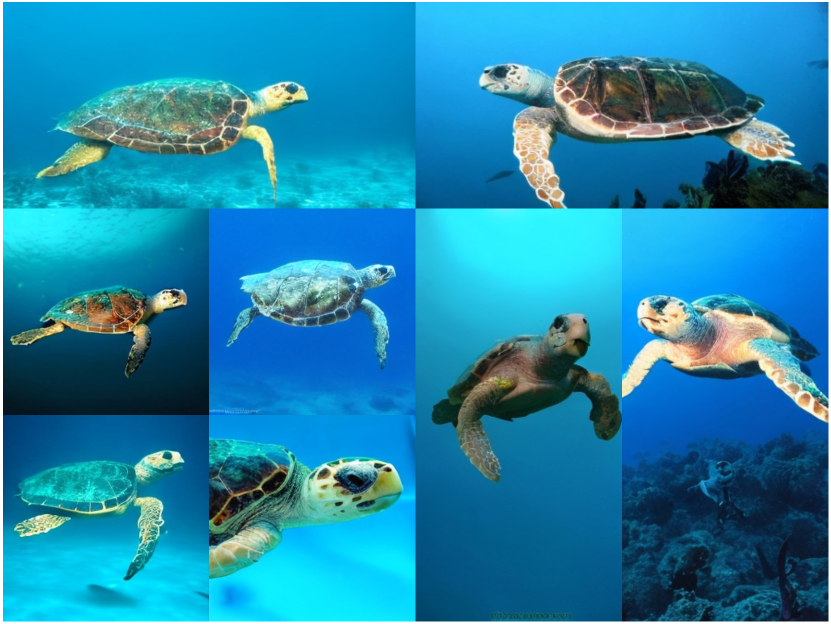
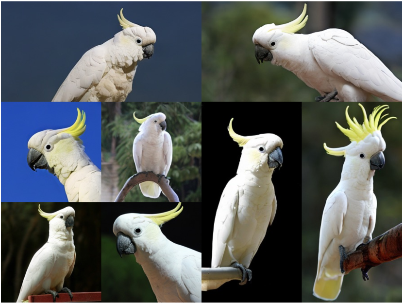
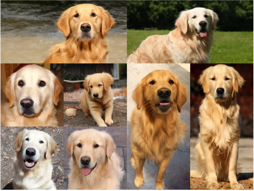
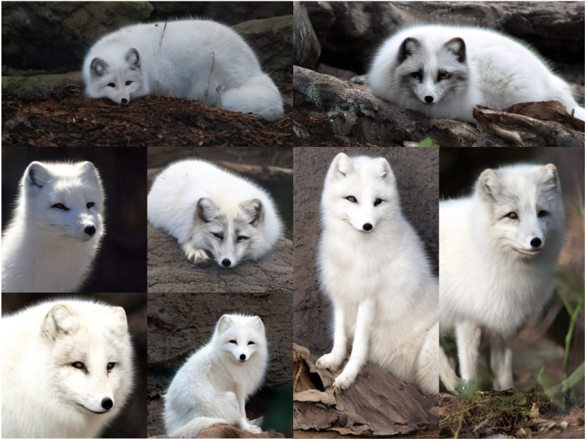
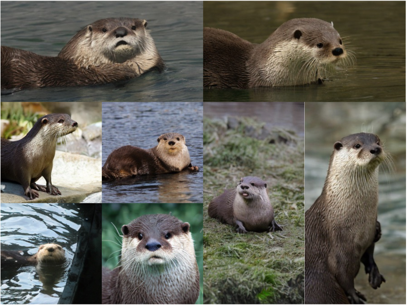
We show samples from our FiT-XL/2 models at resolutions of $256\times 256$, $224\times 448$ and $448\times 224$, trained for 1.8M (generated with 250 DDPM sampling steps and the ft-EMA VAE decoder). Fig. 6 shows uncurated samples from FiT-XL/2 with classifier-free guidance scale 4.0 and class label “loggerhead turtle” (33). Fig. 7 shows uncurated samples from FiT-XL/2 with classifier-free guidance scale 4.0 and class label “Cacatua galerita” (89). Fig. 8 shows uncurated samples from FiT-XL/2 with classifier-free guidance scale 4.0 and class label “golden retriever” (207). Fig. 9 shows uncurated samples from FiT-XL/2 with classifier-free guidance scale 4.0 and class label “white fox” (279). Fig. 10 shows uncurated samples from FiT-XL/2 with classifier-free guidance scale 4.0 and class label “otter” (360). Fig. 11 shows uncurated samples from FiT-XL/2 with classifier-free guidance scale 4.0 and class label “volcano” (980).

We also show some failure samples from DiT-XL/2, as shown in Fig. 5.

Figure 4: Height/Width distribution of the original ImageNet (Deng et al., 2009) dataset.

Figure 5: Uncurated failure samples from DiT-XL/2.

Figure 6: Uncurated samples from FiT-XL/2 models at resolutions of $256\times 256$, $224\times 448$ and $448\times 224$.

Figure 7: Uncurated samples from FiT-XL/2 models at resolutions of $256\times 256$, $224\times 448$ and $448\times 224$.

Figure 8: Uncurated samples from FiT-XL/2 models at resolutions of $256\times 256$, $224\times 448$ and $448\times 224$.

Figure 9: Uncurated samples from FiT-XL/2 models at resolutions of $256\times 256$, $224\times 448$ and $448\times 224$.

Figure 10: Uncurated samples from FiT-XL/2 models at resolutions of $256\times 256$, $224\times 448$ and $448\times 224$.

Figure 11: Uncurated samples from FiT-XL/2 models at resolutions of $256\times 256$, $224\times 448$ and $448\times 224$.

References

- Bao et al. (2023) Bao, F., Nie, S., Xue, K., Cao, Y., Li, C., Su, H., and Zhu, J. All are worth words: A vit backbone for diffusion models. In IEEE/CVF Conference on Computer Vision and Pattern Recognition, 2023.
- Brock et al. (2018) Brock, A., Donahue, J., and Simonyan, K. Large scale gan training for high fidelity natural image synthesis. arXiv preprint arXiv:1809.11096, 2018.
- Brown et al. (2020) Brown, T., Mann, B., Ryder, N., Subbiah, M., Kaplan, J. D., Dhariwal, P., Neelakantan, A., Shyam, P., Sastry, G., Askell, A., et al. Language models are few-shot learners. Advances in Neural Information Processing Systems, 2020.
- Chang et al. (2022) Chang, H., Zhang, H., Jiang, L., Liu, C., and Freeman, W. T. Maskgit: Masked generative image transformer. In Proceedings of the IEEE/CVF Conference on Computer Vision and Pattern Recognition, 2022.
- Chen et al. (2023) Chen, S., Wong, S., Chen, L., and Tian, Y. Extending context window of large language models via positional interpolation. arXiv preprint arXiv:2306.15595, 2023.
- Chowdhery et al. (2023a) Chowdhery, A., Narang, S., Devlin, J., Bosma, M., Mishra, G., Roberts, A., Barham, P., Chung, H. W., Sutton, C., Gehrmann, S., et al. Palm: Scaling language modeling with pathways. Journal of Machine Learning Research, 2023a.
- Chowdhery et al. (2023b) Chowdhery, A., Narang, S., Devlin, J., Bosma, M., Mishra, G., Roberts, A., and et al, P. B. Palm: Scaling language modeling with pathways. Journal of Machine Learning Research, 2023b.
- Dehghani et al. (2023) Dehghani, M., Mustafa, B., Djolonga, J., Heek, J., Minderer, M., Caron, M., Steiner, A., Puigcerver, J., Geirhos, R., Alabdulmohsin, I., et al. Patch n’pack: Navit, a vision transformer for any aspect ratio and resolution. arXiv preprint arXiv:2307.06304, 2023.
- Deng et al. (2009) Deng, J., Dong, W., Socher, R., Li, L.-J., Li, K., and Fei-Fei, L. Imagenet: A large-scale hierarchical image database. In IEEE/CVF Conference on Computer Vision and Pattern Recognition, 2009.
- Dhariwal & Nichol (2021) Dhariwal, P. and Nichol, A. Diffusion models beat gans on image synthesis. Advances in Neural Information Processing Systems, 2021.
- Dosovitskiy et al. (2020) Dosovitskiy, A., Beyer, L., Kolesnikov, A., Weissenborn, D., Zhai, X., Unterthiner, T., Dehghani, M., Minderer, M., Heigold, G., Gelly, S., et al. An image is worth 16x16 words: Transformers for image recognition at scale. arXiv preprint arXiv:2010.11929, 2020.
- Esser et al. (2021) Esser, P., Rombach, R., and Ommer, B. Taming transformers for high-resolution image synthesis. In IEEE/CVF Conference on Computer Vision and Pattern Recognition, 2021.
- Gao et al. (2023) Gao, S., Zhou, P., Cheng, M.-M., and Yan, S. Masked diffusion transformer is a strong image synthesizer. arXiv preprint arXiv:2303.14389, 2023.
- Hatamizadeh et al. (2023) Hatamizadeh, A., Song, J., Liu, G., Kautz, J., and Vahdat, A. Diffit: Diffusion vision transformers for image generation. arXiv preprint arXiv:2312.02139, 2023.
- Heusel et al. (2017) Heusel, M., Ramsauer, H., Unterthiner, T., Nessler, B., and Hochreiter, S. Gans trained by a two time-scale update rule converge to a local nash equilibrium. Advances in Neural Information Processing Systems, 2017.
- Ho & Salimans (2021) Ho, J. and Salimans, T. Classifier-free diffusion guidance. In NeurIPS 2021 Workshop on Deep Generative Models and Downstream Applications, 2021.
- Ho et al. (2020) Ho, J., Jain, A., and Abbeel, P. Denoising diffusion probabilistic models. Advances in Neural Information Processing Systems, 2020.
- Ho et al. (2022) Ho, J., Saharia, C., Chan, W., Fleet, D. J., Norouzi, M., and Salimans, T. Cascaded diffusion models for high fidelity image generation. Journal of Machine Learning Research, 2022.
- Hyvärinen & Dayan (2005) Hyvärinen, A. and Dayan, P. Estimation of non-normalized statistical models by score matching. Journal of Machine Learning Research, 2005.
- Kynkäänniemi et al. (2019) Kynkäänniemi, T., Karras, T., Laine, S., and Lehtinen, J.and Aila, T. Improved precision and recall metric for assessing generative models. Advances in Neural Information Processing Systems, 2019.
- Liu et al. (2023) Liu, X., Yan, H., Zhang, S., An, C., Qiu, X., and Lin, D. Scaling laws of rope-based extrapolation. arXiv preprint arXiv:2310.05209, 2023.
- Liu et al. (2021) Liu, Z., Lin, Y., Cao, Y., Hu, H., Wei, Y., Zhang, Z., Lin, S., and Guo, B. Swin transformer: Hierarchical vision transformer using shifted windows. In IEEE/CVF Conference on Computer Vision and Pattern Recognition, 2021.
- Liu et al. (2022) Liu, Z., Mao, H., Wu, C.-Y., Feichtenhofer, C., Darrell, T., and Xie, S. A convnet for the 2020s. In IEEE/CVF Conference on Computer Vision and Pattern Recognition, 2022.
- (24) LocalLLaMA. Ntk-aware scaled rope allows llama models to have extended (8k+) context size without any fine-tuning and minimal perplexity degradation. https://www.reddit.com/r/LocalLLaMA/comments/14lz7j5/ntkaware_scaled_rope_allows_llama_models_to_have/. Accessed: 2024-2-1.
- Loshchilov & Hutter (2017) Loshchilov, I. and Hutter, F. Decoupled weight decay regularization. arXiv preprint arXiv:1711.05101, 2017.
- Nash et al. (2021) Nash, C., Menick, J., Dieleman, S., and Battaglia, P. W. Generating images with sparse representations. arXiv preprint arXiv:2103.03841, 2021.
- Peebles & Xie (2023) Peebles, W. and Xie, S. Scalable diffusion models with transformers. In IEEE/CVF International Conference on Computer Vision, 2023.
- Peng et al. (2023) Peng, B., Quesnelle, J., Fan, H., and Shippole, E. Yarn: Efficient context window extension of large language models. arXiv preprint arXiv:2309.00071, 2023.
- Radford et al. (2021) Radford, A., Kim, J. W., Hallacy, C., Ramesh, A., Goh, G., Agarwal, S., Sastry, G., Askell, A., Mishkin, P., Clark, J., et al. Learning transferable visual models from natural language supervision. In International Conference on Machine Learning, 2021.
- Rombach et al. (2022) Rombach, R., Blattmann, A., Lorenz, D., Esser, P., and Ommer, B. High-resolution image synthesis with latent diffusion models. In IEEE/CVF Conference on Computer Vision and Pattern Recognition, 2022.
- Ruoss et al. (2023) Ruoss, A., Delétang, G., Genewein, T., Grau-Moya, J., Csordás, R., Bennani, M., Legg, S., and Veness, J. Randomized positional encodings boost length generalization of transformers. arXiv preprint arXiv:2305.16843, 2023.
- Saharia et al. (2022) Saharia, C., Chan, W., Saxena, S., Li, L., Whang, J., Denton, E. L., Ghasemipour, K., Gontijo Lopes, R., Karagol Ayan, B., Salimans, T., et al. Photorealistic text-to-image diffusion models with deep language understanding. Advances in Neural Information Processing Systems, 2022.
- Salimans et al. (2016) Salimans, T., Goodfellow, I., Zaremba, W., Cheung, V., Radford, A., and Chen, X. Improved techniques for training gans. Advances in Neural Information Processing Systems, 2016.
- Sauer et al. (2022) Sauer, A., Schwarz, K., and Geiger, A. Stylegan-xl: Scaling stylegan to large diverse datasets. In ACM SIGGRAPH 2022 conference proceedings, 2022.
- Shazeer (2020) Shazeer, N. Glu variants improve transformer. arXiv preprint arXiv:2002.05202, 2020.
- Song et al. (2020a) Song, J., Meng, C., and Ermon, S. Denoising diffusion implicit models. arXiv preprint arXiv:2010.02502, 2020a.
- Song et al. (2020b) Song, Y., Sohl-Dickstein, J., Kingma, D. P., Kumar, A., Ermon, S., and Poole, B. Score-based generative modeling through stochastic differential equations. arXiv preprint arXiv:2011.13456, 2020b.
- Su et al. (2024) Su, J., Ahmed, M., Lu, Y., Pan, S., Bo, W., and Liu, Y. Roformer: Enhanced transformer with rotary position embedding. Neurocomputing, 2024.
- Sun et al. (2022) Sun, Y., Dong, L., Patra, B., Ma, S., Huang, S., Benhaim, A., Chaudhary, V., Song, X., , and Wei, F. A length-extrapolatable transformer. arXiv preprint arXiv:2212.10554, 2022.
- Team et al. (2023) Team, G., Anil, R., Borgeaud, S., Wu, Y., Alayrac, J.-B., Yu, J., Soricut, R., Schalkwyk, J., Dai, A. M., Hauth, A., et al. Gemini: a family of highly capable multimodal models. arXiv preprint arXiv:2312.11805, 2023.
- Touvron et al. (2019) Touvron, H., Vedaldi, A., Douze, M., and Jégou, H. Fixing the train-test resolution discrepancy. Advances in Neural Information Processing Systems, 2019.
- Touvron et al. (2021) Touvron, H., Cord, M., Douze, M., Massa, F., Sablayrolles, A., and Jégou, H. Training data-efficient image transformers & distillation through attention. In International conference on machine learning, pp. 10347–10357. PMLR, 2021.
- Touvron et al. (2023a) Touvron, H., Lavril, T., Izacard, G., Martinet, X., Lachaux, M.-A., Lacroix, T., and et al, B. R. Llama: Open and efficient foundation language models. arXiv preprint arXiv:2302.13971, 2023a.
- Touvron et al. (2023b) Touvron, H., Martin, L., Stone, K., Albert, P., Almahairi, A., Babaei, Y., and et al, N. B. Llama 2: Open foundation and fine-tuned chat models. arXiv preprint arXiv:2307.09288, 2023b.
- Vaswani et al. (2017) Vaswani, A., Shazeer, N., Parmar, N., Uszkoreit, J., Jones, L., Gomez, A. N., Kaiser, Ł., and Polosukhin, I. Attention is all you need. Advances in Neural Information Processing Systems, 2017.