Universal Physics Transformers

Abstract

Deep neural network based surrogates for partial differential equations have recently gained increased interest. However, akin to their numerical counterparts, different techniques are used across applications, even if the underlying dynamics of the systems are similar. A prominent example is the Lagrangian and Eulerian specification in computational fluid dynamics, posing a challenge for neural networks to effectively model particle- as opposed to grid-based dynamics. We introduce Universal Physics Transformers (UPTs), a novel learning paradigm which models a wide range of spatio-temporal problems – both for Lagrangian and Eulerian discretization schemes. UPTs operate without grid- or particle-based latent structures, enabling flexibility across meshes and particles. UPTs efficiently propagate dynamics in the latent space, emphasized by inverse encoding and decoding techniques. Finally, UPTs allow for queries of the latent space representation at any point in space-time. We demonstrate the efficacy of UPTs in mesh-based fluid simulations, steady-state Reynolds averaged Navier-Stokes simulations, and Lagrangian-based dynamics. Project page: https://ml-jku.github.io/UPT

1 Introduction

In scientific pursuits, extensive efforts have produced highly intricate mathematical models of physical phenomena, many of which are naturally expressed as partial differential equations (PDEs) (Olver, 2014). Nevertheless, solving most PDEs is analytically intractable and necessitates falling back on compute-expensive numerical approximation schemes. In recent years, deep neural network based surrogates have surged, emerging as a computationally efficient alternative (Thuerey et al., 2021; Zhang et al., 2023), and impacting e.g., weather forecasting (Lam et al., 2022; Bi et al., 2022; Andrychowicz et al., 2023), molecular modeling (Batzner et al., 2022; Batatia et al., 2022), or computational fluid dynamics (Vinuesa & Brunton, 2022; Guo et al., 2016; Li et al., 2020a; Kochkov et al., 2021; Gupta & Brandstetter, 2022; Carey et al., 2024). Additional to computational efficiency, neural surrogates offer potential to introduce generalization capabilities across phenomena, as well as generalization across characteristics such as boundary conditions or PDE coefficients (Brandstetter et al., 2022c). Therefore, the nature of neural surrogates inherently complements handcrafted numerical solvers which are characterized by a substantial set of solver requirements, and mostly due to these requirements tend to differ among sub-problems (Bartels, 2016). However, similar to their numerical counterparts, different neural network techniques are applied across applications. Presumably the biggest difference comes when contrasting moving particle and grid-based dynamics in computational fluid dynamics (CFD), i.e., Lagrangian and Eulerian discretization schemes. On the one hand, the Lagrangian specification of the flow field tracks individual fluid particles, describing their properties as they move through space and time. In Eulerian specification, on the other hand, fluid properties like velocity and pressure are observed at fixed points in a stationary grid.

\begin{overpic}[width=433.62pt]{resources/schematics/upt_sketch_no_text.pdf} \par \put(60.0,19.0){{Encoder}} \put(148.0,19.0){{Approximator}} \put(250.0,19.0){{Decoder}} \par\put(155.0,86.0){{Features}} \put(155.0,78.0){{Position}} \put(155.0,69.0){{Latent Token}} \par\put(155.0,53.0){{Repeat until }$t^{\prime}$} \par\put(9.0,130.0){{Discretized Eulerian / Lagrangian Data at }$t$} \put(200.0,130.0){{Discretized Eulerian / Lagrangian Data at }$t^{\prime}$} \par\put(320.0,60.0){{Positions to Query at}} \end{overpic}

Figure 1: Schemantic sketch of the UPT learning paradigm. UPTs flexible encode different grids, and/or different number of particles into a unified latent space representation, and subsequently unroll dynamics in the latent space. The latent space is kept at a fixed size to ensure scalability to larger systems. UPTs decode the latent representation at any query point.

A seemingly great fit for particle-based dynamics are graph neural networks (GNNs) (Scarselli et al., 2008; Kipf & Welling, 2017) with graph-based latent space representations. In many cases, predicted accelerations at the nodes are numerically integrated to model the time evolution of the many-particle systems (Sanchez-Gonzalez et al., 2020; Mayr et al., 2023; Toshev et al., 2023a, 2024). In contrast, grid-based problems are often modeled – as the name suggests – on a fixed grid or a fixed mesh. Recently the neural operator learning paradigm has emerged which learns a mapping between infinite dimensional function spaces (Li et al., 2020a; Lu et al., 2021; Kovachki et al., 2021), e.g., flow fields. Most state-of-the-art neural operator methods work on regular grids, e.g., Li et al. (2020a), learn a mapping to a uniform mesh, e.g., Li et al. (2023), or rely on tokenizend latent space representations, e.g., Hao et al. (2023).

We introduce Universal Physics Transformers (UPTs), a novel learning paradigm for a wide range of spatio-temporal problems in computational fluid dynamics. UPTs seamlessly operate on both Lagrangian and Eulerian discretization schemes. UPTs flexibly encode different grids, and/or different number of particles into a unified latent space representation, and subsequently unroll dynamics in the latent space. The latent dynamics are guided by scene representations and problem-dependent surrogate information. Latent space rollouts are enforced by inverse encoding and decoding surrogates, leading to fast and stable simulated trajectories. For decoding, the latent representation can be evaluated at any point in space-time. UPTs operate without grid- or particle-based latent structures, and demonstrate the beneficial scaling-behavior of transformer backbone architectures. Figure 1 sketches the UPT modeling paradigm.

We demonstrate the efficacy of UPTs in mesh-based fluid simulations, steady-state Reynolds averaged Navier-Stokes simulations, and Lagrangian-based dynamics

2 Background

Partial differential equations

In this work, we focus on experiments on (systems of) PDEs, that evolve a signal $\bm{u}(t,\bm{x})=\bm{u}^{t}(\bm{x})\in\mathbb{R}^{d}$ in a single temporal dimension $t\in[0,T]$ and $m$ spatial dimensions $\bm{x}\in U\subset\mathbb{R}^{m}$, for an open set $U$. With $1\leq l\in\mathbb{N}$, systems of PDEs of order $l$ can be written as

$$\bm{F}(D^{l}\bm{u}^{t}(\bm{x}),\ldots,D^{1}\bm{u}^{t}(\bm{x}),\frac{\partial^{l}}{\partial t^{l}}\bm{u}^{t}(\bm{x}),\ldots,\frac{\partial}{\partial t}\bm{u}^{t}(\bm{x}),\bm{u}^{t}(\bm{x}),\bm{x},t)=\mathbf{0},\ \ \ \ \text{for }\bm{x}\in U,\ t\in[0,T]\ ,$$ (1)

where $\bm{F}$ is a mapping to $\mathbb{R}^{d}$, and for $i=1,...,l$, $D^{i}$ denotes the differential operator mapping to all $i$-th order partial derivatives of $\bm{u}$ with respect to the spacial variable $\bm{x}$, whereas $\frac{\partial^{i}}{\partial t^{i}}$ outputs the corresponding time derivative of order $i$. Any $l$-times continuously differentiable $\bm{u}:[0,T]\times U\rightarrow\mathbb{R}^{d}$ fulfilling the relation Eq. (1) is called a classical solution of Eq. (1). Also other notions of solvability (e.g. in the sense of weak derivatives/distributions) are possible, for sake of simplicity we do not go into details here. Additionally, initial conditions specify $\bm{u}^{t}(\bm{x})$ at time $t=0$ and boundary conditions $B[\bm{u}^{t}](\bm{x})$ at the boundary of the spatial domain.

We work mostly with the incompressible Navier-Stokes equations (Temam, 2001), which e.g., in two spatial dimensions conserve the velocity flow field $\bm{u}(t,x,y):[0,T]\times\mathbb{R}^{2}\rightarrow\mathbb{R}^{2}$ via:

$$\frac{\partial\bm{u}}{\partial t}=-\bm{u}\cdot\nabla\bm{u}+\mu\nabla^{2}\bm{u}-\nabla p+\bm{f}\ ,\quad\nabla\cdot\bm{u}=0\ ,$$ (2)

where $\bm{u}\cdot\nabla\bm{u}$ is the convection, i.e., the rate of change of $\bm{u}$ along $\bm{u}$, $\mu\nabla^{2}\bm{u}$ the viscosity, i.e., the diffusion or net movement of $\bm{u}$, $\nabla p$ the internal pressure gradient, and $\bm{f}$ an external force. The constraint $\nabla\cdot\bm{u}=0$ yields mass conservation of the Navier-Stokes equations. A detailed depiction of the involved differential operators is given in Appendix A.1.

Operator learning

Operator learning (Lu et al., 2019, 2021; Li et al., 2020b, a; Kovachki et al., 2021) learns a mapping between function spaces, and this concept is often used to approximate solutions of PDEs. Similar to Kovachki et al. (2021), we assume $\mathcal{U},\mathcal{V}$ to be Banach spaces of functions on compact domains $\mathcal{X}\subset\mathbb{R}^{d_{x}}$ or $\mathcal{Y}\subset\mathbb{R}^{d_{y}}$, mapping into $\mathbb{R}^{d_{u}}$ or $\mathbb{R}^{d_{v}}$, respectively. The goal of operator learning is to learn a ground truth operator $G:\mathcal{U}\rightarrow\mathcal{V}$ via an approximation $\hat{{\mathcal{G}}}:\mathcal{U}\rightarrow\mathcal{V}$. This is usually done in the vein of supervised learning by i.i.d. sampling input-output pairs, with the notable difference, that in operator learning the spaces sampled from are not finite dimensional. More precisely, with a given data set consisting of $N$ function pairs $(\bm{u}_{i},\bm{v}_{i})=(\bm{u}_{i},{\mathcal{G}}(\bm{u}_{i}))\subset\mathcal{U}\times\mathcal{V}$, $i=1,...N$, we aim to learn $\hat{{\mathcal{G}}}:\mathcal{U}\rightarrow\mathcal{V}$, so that ${\mathcal{G}}$ can be approximated in a suitably chosen norm.

In the context of PDEs, ${\mathcal{G}}$ can e.g. be the mapping from an initial condition $\bm{u}(0,\bm{x})=\bm{u}^{0}(\bm{x})$ to the solutions $\bm{u}(t,\bm{x})=\bm{u}^{t}(\bm{x})$ of Eq. (1) at all times. In the case of classical solutions, if $U$ is bounded, $\mathcal{U}$ can then be chosen as a subspace of $C(\bar{U},\mathbb{R}^{d})$, the set of continuous functions from domain $\bar{U}$ (the closure of $U$) mapping to $\mathbb{R}^{d}$, whereas $\mathcal{V}\subset C([0,T]\times\bar{U},\mathbb{R}^{d})$, so that $\mathcal{U}$ or $\mathcal{V}$ consist of all $l$-times continuosly differentiable functions on the respective spaces. In case of weak solutions, the associated spaces $\mathcal{U}$ and $\mathcal{V}$ can be chosen as Sobolev spaces.

A popular approach, that we are also going to follow, is to approximate ${\mathcal{G}}$ via three maps (Seidman et al., 2022): ${\mathcal{G}}\approx\hat{{\mathcal{G}}}\coloneqq\mathcal{D}\circ\mathcal{A}\circ\ \mathcal{E}.$ The encoder $\mathcal{E}:\mathcal{U}\rightarrow\mathbb{R}^{h_{1}}$ takes an input function and maps it to a finite dimensional latent feature representation. For example, $\mathcal{E}$ could embed a continuous function to a chosen hidden dimension $\mathbb{R}^{h_{1}}$ for a collection of grid points. Next, $\mathcal{A}:\mathbb{R}^{h_{1}}\rightarrow\mathbb{R}^{h_{2}}$ approximates the action of the operator $\mathcal{G}$, and $\mathcal{D}$ decodes the hidden representation, and thus creates the output functions via $\mathcal{D}:\mathbb{R}^{h_{2}}\rightarrow\mathcal{V}$, which in many cases is point-wise evaluated at the output grid or output mesh.

Particle vs. grid-based methods

Often, numerical simulation methods can be classified into two distinct families: particle and grid-based methods. This specification is notably prevalent, for instance, in the field of computational fluid dynamics (CFD), where Lagrangian and Eulerian discretization schemes offer different characteristics dependent on the PDEs. In simpler terms, Eulerian schemes essentially monitor velocities at specific fixed grid points. These points, represented by a spatially limited number of nodes, control volumes, or cells, serve to discretize the continuous space. This process leads to grid-based or mesh-based representations. In contrast to such grid- and mesh-based representations, in Lagrangian schemes, the discretization is carried out using finitely many material points, often referred to as particles, which move with the local deformation of the continuum. Roughly speaking, there are three families of Lagrangian schemes: discrete element methods (Cundall & Strack, 1979), material point methods (Sulsky et al., 1994; Brackbill & Ruppel, 1986), and smoothed particle hydrodynamics (SPH) (Gin, 1977; Lucy, 1977; Monaghan, 1992, 2005). In this work, we focus on SPH methods, which approximate the field properties using radial kernel interpolations over adjacent particles at the location of each particle. The strength of SPH lies in its ability to operate without being constrained by connectivity issues, such as meshes. This characteristic proves especially beneficial when simulating systems that undergo significant deformations.

Latent space representation of neural operators

For larger meshes or larger number of particles, memory consumption and inference speed become more and more important. Fourier Neural Operator (FNO) based methods work on regular grids, or learn a mapping to a regular latent grid, e.g., geometry-informed neural operators (GINO) (Li et al., 2023). In three dimensions, the stored Fourier modes have the shape $h\times n_{x}\times n_{y}\times n_{z}$, where $h$ is the hidden size and $n_{x}$, $n_{y}$, $n_{z}$ are the respective Fourier modes. Similarly, the latent space of CNN-based methods, e.g., Raonić et al. (2023); Gupta & Brandstetter (2022), is of shape $h\times w_{x}\times w_{y}\times w_{z}$, where $w_{x}$, $w_{y}$, $w_{z}$ are the respective grid points. In three dimension, the memory requirement in each layer increases cubically with increasing number of modes or grid points. In contrast, transformer based neural operators, e.g., Hao et al. (2023); Cao (2021); Li et al. (2022b), operate on a token-based latent space of dimension $n_{\text{tokens}}\times h$, where usually $n_{\text{tokens}}\propto n_{\text{points}}$, and GNN based neural operators, e.g., Li et al. (2020b), operate on a node based latent space of dimension $n_{\text{nodes}}\times h$, where usually $n_{\text{nodes}}=n_{\text{points}}$. While these methods offer a more cost-effective memory footprint, the computational demand, particularly in the case of self-attention, rises quadratically with the number of tokens. Different architectures are compared in Tab. 1.

Model	Range	Complexity	Irregular	Discretization	Learns	Latent
			Grid	Convergent	Field	Rollout
GNN	local	$O(MD)$	✓	✗	✗	✗
CNN	local	$O(G)$	✗	✗	✗	✗
Transformer	global	$O(M^{2})$	✓	✓	✗	✗
GNO (Li et al., 2020b)	radius	$O(MD)$	✓	✓	✗	✗
FNO (Li et al., 2020a)	global	$O(G\log G)$	✗	✓	✗	✗
GINO (Li et al., 2023)	global	$O(GD+G\log G)$	✓	✓	✓	✗
UPT (with GNO)	global	$O(SD+S^{2})$	✓	✓	✓	✓
UPT (without GNO)	global	$O(SM+S^{2})$	✓	✓	✓	✓

Table 1: Model comparison. Complexity includes number of mesh points $M$, and maximum degree of the graph $D$. Grid-based methods project the mesh to $G$ grid points. UPTs instead use a small amount of supernodes $S$ as discretization, where $G$ is typically much larger than $S$. The UPT training procedure separates responsibilities between components, allowing us to forward propage dynamics purely within the latent space. For large meshes, UPT uses a GNO to compress the mesh points into supernodes (“with GNO”), which can be omitted for small meshes (“without GNO”).

3 Universal Physics Transformers

Problem formulation

Our goal is to learn a mapping between the solutions $\bm{u}^{t}$ and $\bm{u}^{t^{\prime}}$ of Eq. (1) at timesteps $t$ and $t^{\prime}$, respectively. Our dataset should consist of $N$ function pairs $(\bm{u}^{t}_{i},\bm{u}^{t^{\prime}}_{i})$, $i=1,..,N$, where each $\bm{u}^{t}_{i}$ is sampled at $k$ spatial locations $\{\bm{x}^{1}_{i},\ldots,\bm{x}^{k}_{i}\}\in U$. Similarly, we query each output signal $\hat{\bm{u}}^{t^{\prime}}_{i}$ at $k^{\prime}$ spatial locations $\{\bm{y}^{1}_{i},\ldots,\bm{y}^{k^{\prime}}_{i}\}\in U$. Then each input signal can be represented by $\bm{u}_{i,k}^{t}=(\bm{u}_{i}^{t}(\bm{x}^{1}_{i}),\ldots,\bm{u}_{i}^{t}(\bm{x}^{k}_{i}))^{T}\in\mathbb{R}^{k\times d}$ as a tensor of shape $k\times d$, similar for the output. For particle- or mesh-based inputs, it is often simpler to represent the input as graph $\mathscr{G}=(V,E)$ with $k$ nodes $\{\bm{x}^{1}_{i},\ldots\bm{x}^{k}_{i}\}\in V$, edges $E$ (that reflect the neighborhood structure) and node features $\{\bm{u}^{t}_{i}(\bm{x}^{1}_{i}),\ldots,\bm{u}^{t}_{i}(\bm{x}^{k}_{i})\}$.

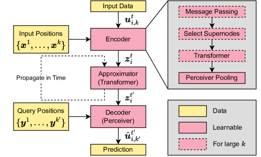
Figure 2: Schemantic sketch of the UPT architecture. The encoder compresses information from various grids or differing particles. Subsequently, this information is propagated forward in time through the approximator and decoded at arbitrary query positions.

Architecture desiderata

We want Universal Physics Transformers (UPTs) to fulfill the following set of desiderata: (i) an encoder $\mathcal{E}$, which flexibly encodes different grids, and/or different number of particles into a unified latent representation of shape $n_{\text{latent}}\times h$, where $n_{\text{latent}}$ is the chosen number of tokens in the latent space and $h$ is the hidden dimension; (ii) an approximator $\mathcal{A}$ and a training procedure, which allows us to forward propagate dynamics purely within the latent space without mapping back to the spatial domain at each operator step; and iii) a decoder $\mathcal{D}$ that queries the latent representation at different locations. The UPT architecture is schematically sketched in Fig. 2.

Encoder

The goal of the encoder $\mathcal{E}$ is to compress the input signal $\bm{u}_{i}^{t}$, which is represented by a point cloud $\bm{u}_{i,k}^{t}$. Importantly, the encoder should learn to selectively focus on important parts of the input. This is a desirable property as, for example, in many computational fluid dynamics simulations large areas are characterized by laminar flows, whereas turbulent flows tend to occur especially around obstacles. If $k$ is large, we employ a hierarchical encoder.

The encoder $\mathcal{E}$ first embeds $k$ points into hidden dimension $h$, adding position encoding (Vaswani et al., 2017) to the different nodes, i.e., $\bm{u}_{i,k}^{t}\in\mathbb{R}^{k\times d}\rightarrow\mathbb{R}^{k\times h}$. In the first hierarchy, information is exchanged between local points and a selected set of $n_{\text{s}}$ supernode points. For Eulerian discretization schemes those supernodes can either be uniformly sampled on a regular grid as in Li et al. (2023), or selected based on the given mesh. The latter has the advantage that mesh characteristics are automatically taken into account, e.g., dense or sparse mesh regions are represented by different numbers of nodes. Furthermore, adaptation to new meshes is straightforward. We implement the first hierarchy by randomly selecting $n_{\text{s}}$ supernodes on the mesh, choosing $n_{\text{s}}$ such that the mesh characteristic is preserved. E.g., for experiments presented in Sec. 4.2, $n_{\text{s}}=2048$. Similarly, in the Lagrangian discretization scheme, choosing supernodes based on particle positions provides the same advantages as selecting them based on the mesh.

Information is aggregated at the selected $n_{\text{s}}$ supernodes via a message passing layer (Gilmer et al., 2017) using a radius graph between points. Importantly, messages only flow towards the $n_{\text{s}}$ supernodes, and thus the compute complexity of the first hierarchy scales linearly with $n_{\text{s}}$. The second hierarchy consists of transformer blocks (Vaswani et al., 2017) followed by a perceiver block (Jaegle et al., 2021b, a) with $n_{\text{latent}}$ learned queries of dimension $h$. To summarize, the encoder $\mathcal{E}$ maps $\bm{u}_{i}^{t}\in\mathcal{U}$ to a latent space via

$$\mathcal{E}:\bm{u}_{i}^{t}\in\mathcal{U} \xrightarrow[]{\text{evaluate}}\bm{u}_{i,k}^{t}\in\mathbb{R}^{k\times d}\xrightarrow[]{\text{embed}}\mathbb{R}^{k\times h}\xrightarrow[]{\text{MP}}\mathbb{R}^{n_{s}\times h}$$

$$\xrightarrow[]{\text{transformer}}\mathbb{R}^{n_{s}\times h}\xrightarrow[]{\text{perceiver}}\bm{z}^{t}_{i}\in\mathbb{R}^{n_{\text{latent}}\times h}\ ,$$

where tyically $n_{\text{latent}}\ll n_{\text{s}}<k$. If the number of points is manageable, the first hierarchy can be omitted.

Approximator

The approximator propagates the compressed representation forward in time. As $n_{\text{latent}}$ is small, forward propagation in time is fast. We employ a stack of transformer blocks as approximator.

$$\mathcal{A}:\bm{z}^{t}_{i}\in\mathbb{R}^{n_{\text{latent}}\times h}\rightarrow\bm{z}^{t^{\prime}}_{i}\in\mathbb{R}^{n_{\text{latent}}\times h}\ .$$

Notably, the approximator can be applied multiple times, propagating the input signal forward in time by $\Delta t$ each time. If $\Delta t$ is small enough, the input signal can be approximated at arbitrary future times $t^{\prime}$.

Decoder

The task of decoder $\mathcal{D}$ is to query the latent representation at $k^{\prime}$ arbitrary locations to construct the prediction of the output signal $\bm{u}_{i}^{t^{\prime}}$ at time $t^{\prime}$. More formally, given the output positions $\{\bm{y}^{1}_{i},\ldots,\bm{y}^{k^{\prime}}_{i}\}\in U$ at $k^{\prime}$ spatial locations and the latent representation $\bm{z}^{t^{\prime}}_{i}$, the decoder predicts the output signal $\bm{u}_{i,k^{\prime}}^{t^{\prime}}=(\bm{u}_{i}^{t^{\prime}}(\bm{y}^{1}_{i}),\ldots,\bm{u}_{i}^{t^{\prime}}(\bm{y}^{k^{\prime}}_{i}))^{T}$ at these spatial locations at timestep $t^{\prime}$,

$$\mathcal{D}:(\bm{z}^{t^{\prime}}_{i},\{\bm{y}^{1}_{i},\ldots,\bm{y}^{k^{\prime}}_{i}\})\rightarrow\hat{\bm{u}}_{i,k^{\prime}}^{t^{\prime}}\in\mathbb{R}^{k^{\prime}\times d}\ .$$

The decoder is implemented via a perceiver-like cross attention layer using a positional embedding of the output positions as query and the latent representation $\bm{z}_{i}^{t^{\prime}}$ as keys and values. Since there is no interaction between queries, the latent representation can be queried at arbitrarily many positions without large computational overhead.

Model Conditioning

To condition the model to the current timestep $t$ and to boundary conditions such as the inflow velocity, we add feature modulation to all transformer and perceiver blocks. We use DiT modulation (Li et al., 2022a), which consists of a dimension-wise scale, shift and gate operation that are applied to the attention and MLP module of the transformer. Scale, shift and gate are dependent on an embedding of the timestep and boundary conditions.

Training procedure

UPTs model the dynamics fully within a latent representation, such that during inference only the initial state of the system $\bm{u}(0,\bm{x})=\bm{u}^{0}(\bm{x})$ is encoded into a latent representation $\bm{z}^{0}$. From there on, instead of autoregressively feeding the decoder’s prediction into the encoder, UPTs propagate $\bm{z}^{0}$ forward in time to $\bm{z}^{t^{\prime}}$ through iteratively applying the approximator $\mathcal{A}$ in the latent space. We call this procedure latent rollout. Especially for large meshes or many particles, the benefits of latent space rollouts, i.e. fast inference, pays off.

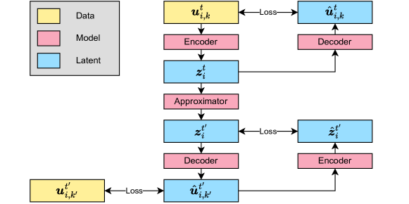
Figure 3: UPT training procedure to enable latent rollouts. To separate the responsibilities of the individual components, we introduce inverse encoding and decoding losses in addition to the next step prediction loss.

To enable latent rollouts, the responsibilities of encoder $\mathcal{E}$, approximator $\mathcal{A}$ and decoder $\mathcal{D}$ need to be isolated. Therefore, we invert the encoding and decoding by means of two reconstruction losses during training as visualized in Fig. 3. First, an inverse encoding is performed, wherein the input $\bm{u}_{i}^{t}$ is reconstructed from the encoded latent state $\bm{z}^{t}_{i}$ by querying it with the decoder at $k$ input locations $\{\bm{x}^{1}_{i},\ldots,\bm{x}^{k}_{i}\}$. Second, we invert the decoding by reconstructing the latent state $\bm{z}^{t^{\prime}}_{i}$ from the output signal $\hat{\bm{u}}^{t^{\prime}}_{i}$ at $k^{\prime}$ spatial locations $\{\bm{y}^{1}_{i},\ldots,\bm{y}^{k^{\prime}}_{i}\}$. Using two reconstruction losses, the encoder is forced to focus on encoding a state $\bm{u}^{t}_{i}$ into a latent representation $\bm{z}^{t}$, and similarly the decoder is forced to focus on making predictions out of a latent representation $\bm{z}^{t^{\prime}}$.

Related methods

The closest work to ours are transformer neural operators of Cao (2021); Li et al. (2022b); Hao et al. (2023) which encode different query points into a tokenized latent space representation of dimension $n_{\text{nodes}}\times h$, where $n_{\text{nodes}}$ varies based on the number of input points, i.e., $n_{\text{nodes}}\propto n_{\text{points}}$. Wu et al. (2024) adds a learnable mapping into a fixed latent space of dimension $n_{\text{nodes}}\times h$ to each transformer layer, and projects back to dimension $n_{\text{points}}\times h$ after self-attention. In contrast, UPTs use fixed $n_{\text{latent}}$ for the unified latent space representation $n_{\text{latent}}\times h$.

For the modeling of temporal PDEs, a common scheme is to map the input solution at time $t$ to the solution at next time step $t^{\prime}$ (Li et al., 2020a; Brandstetter et al., 2022a; Takamoto et al., 2022). Especially for systems that are modeled by graph-based representations, predicted accelerations at nodes are numerically integrated to model the time evolution of the system (Sanchez-Gonzalez et al., 2020; Pfaff et al., 2020). Recently, equivariant graph neural operators (Xu et al., 2024) were introduced which model time evolution via temporal convolutions in Fourier space. More related to our work are methods that propagate dynamics in the latent space (Lee & Carlberg, 2021; Wiewel et al., 2019). Once the system is encoded, time evolution is modeled via LSTMs (Wiewel et al., 2019), or even linear propagators (Lusch et al., 2018; Morton et al., 2018). In Li et al. (2022b), attention-based layers are used for encoding the spatial information of the input and query points, while time updates in the latent space are performed using recurrent MLPs. Similarly, Bryutkin et al. (2024) use recurrent MLPs for temporal updates within the latent space, while utilizing a graph transformer for encoding the input observations.

Building universal models aligns with the contemporary trend of foundation models for science. Recent works comprise pretraining over multiple heterogeneous physical systems, mostly in the form of PDEs (McCabe et al., 2023), foundation models for weather and climate (Nguyen et al., 2023), or material modeling (Merchant et al., 2023; Zeni et al., 2023; Batatia et al., 2022).

Methods similar to our latent space modeling have been proposed in the context of diffusion models (Rombach et al., 2022) where a pre-trained compression model is used to compress the input into a latent space from which a diffusion model can be trained at much lower costs. Similarly, our approach also compresses the high-dimensional input into a low-dimensional latent space, but without relying on a two stage approach. Instead, we learn the compression end-to-end via inverse encoding and decoding techniques.

4 Experiments

We ran experiments across different settings, assessing three key aspects of UPTs: (i) Effectiveness of the latent space representation. We test on steady state flow simulations in three dimensions, comparing against methods that use regular grid representations, and thus considerably larger latent space representations. (ii) Scalability. We test on transient flow simulations on large meshes. Specifically, we test the effectiveness of latent space rollouts, and assess how well UPTs generalize across different flow regime, and different domains, i.e., different number of mesh points and obstacles. (iii) Lagrangian dynamics modeling. Finally, we assess how well UPTs model underlying field characteristics when applied to particle-based simulations.

4.1 Steady state flows

For steady state prediction, we consider the dataset generated by Umetani & Bickel (2018), which we denote as ShapeNet-Car. It consists of 889 car shapes from ShapeNet (Chang et al., 2015), where each car surface is represented by 3.6K mesh points in 3D space. Umetani & Bickel (2018) simulated 10 seconds of air flow and averaged the results over the last 4 seconds (see Appendix A.3.1 for more information on Reynolds-averaged Navier-Stokes (RANS) equations). The inflow velocity is fixed at $20~{}\text{m}/\text{s}$ with an estimated Reynolds Number of $\text{Re}=5\times 10^{6}$. Following GINO (Li et al., 2023), we randomly split the data into 700 training samples and 189 test samples. We regress the pressure at each surface point with a mean-squared error (MSE) loss and sweep hyperparameters per model. Note that due to the small scale of this dataset, we train the largest possible model that is able to generalize the best. Training even larger models resulted in a performance decrease due to overfitting. We optimize the model size for all methods where the best mesh based models (GINO, UPT) contain around 300M parameters. The best regular grid based models (U-Net (Ronneberger et al., 2015; Gupta & Brandstetter, 2022), FNO (Li et al., 2020a)) are significantly smaller and range from 15M to 100M. Additional details are listed in Appendix B.3.

In GINO, feature engineering in the form of a signed distance function (SDF) is used in addition to the mesh points to represent the irregular mesh as a regular grid. To include these features into UPT, we encode them into $8^{3}=512$ latent SDF tokens using a shallow ConvNeXt V2 (Woo et al., 2023). These SDF tokens are concatenated to the latent tokens produced by the encoder and then fed to the approximator. When using the SDF features, we chose $n_{\text{latent}}=1024$ to balance the number of tokens from the mesh with the number of SDF tokens. Without SDF tokens, a much smaller number of tokens (64) is used. Implementation details and more information on the baseline models are provided in Appendix B.3.

ShapeNet-Car is a small-scale dataset. Consequently, methods that map the mesh onto a regular grid can employ grids of extremely high resolution, such that the number of grid points is orders of magnitude higher than the number of mesh points.. For example, a grid resolution of 64 points per spatial dimension results in 262.114 grid points, which is 73x the number of mesh points. As UPT is designed to operate directly on the mesh, we compare at different grid resolutions. The results in Tab. 2 demonstrate that UPT can model the underlying dynamics with a fraction of latent tokens and performs best across all grid sizes except at the highest resolution of $64^{3}$ where GINO performs slightly better.

Model	SDF	#Tokens	MSE	Mem. [GB]
U-Net	0	$64^{3}$	6.13	1.3
FNO	0	$64^{3}$	4.04	3.8
GINO	0	$64^{3}$	2.34	19.8
UPT (ours)	0	$64$	2.31	0.6
U-Net	32	$32^{3}$	3.66	0.2
FNO	32	$32^{3}$	3.31	0.5
GINO	32	$32^{3}$	2.90	2.1
UPT (ours)	32	$8^{3}+1024$	2.35	2.7
U-Net	64	$64^{3}$	2.83	1.3
FNO	64	$64^{3}$	3.26	3.8
GINO	64	$64^{3}$	2.14	19.8
UPT (ours)	64	$8^{3}+1024$	2.24	2.7

Table 2: Normalized test MSE for ShapeNet-Car pressure prediction. The loss is multiplied by 100. Memory denotes the amount required for a forward and backward pass of a single sample. UPTs can model the dynamics with a fraction of latent tokens compared to other models.

4.2 Transient flows

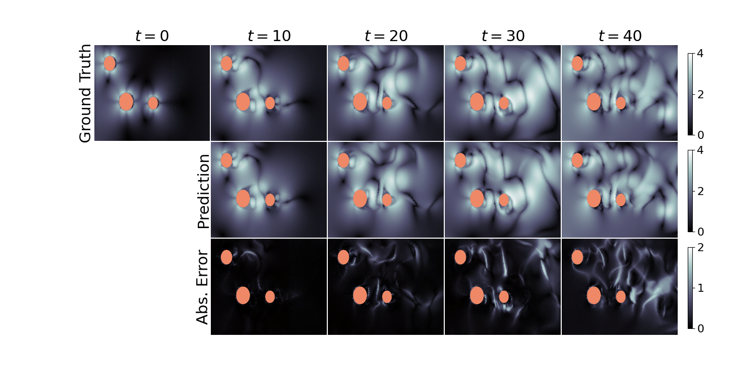
Figure 4: Example rollout trajectories of the UPT-68M model, visually demonstrating the efficacy of UPT physics modeling. The UPT model is trained across different obstacles, different flow regimes, and different mesh discretizations. Interestingly, the absolute error might suggest that UPT trajectories diverge, although physics are still simulated faithfully. This stems from subtle shifts in predictions throughout the rollout duration, likely attributed to the point-wise decoding of the latent field.

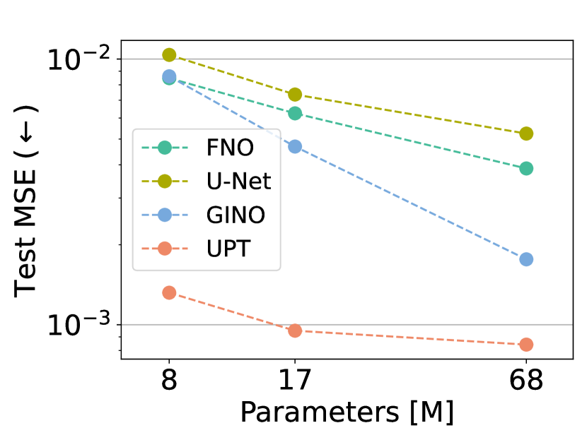
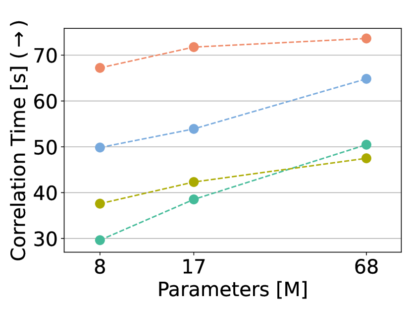
Figure 5: Transient flow results. MSE and correlation time on the testset. UPTs outperform compared methods on all model scales by a large margin.

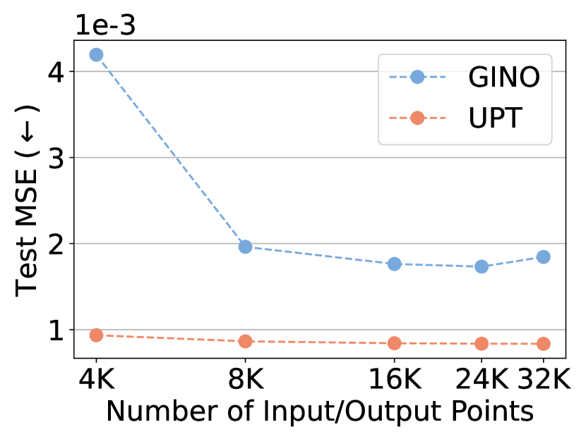
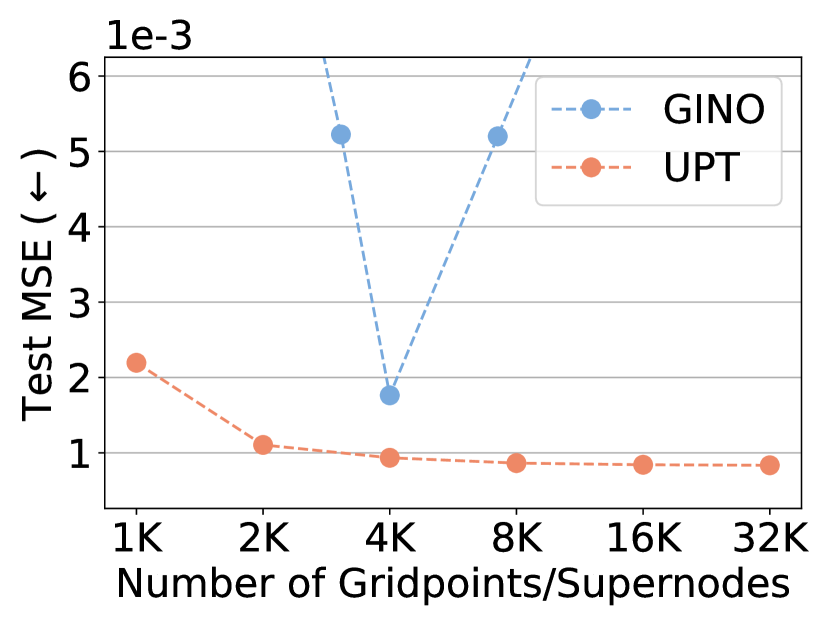
Figure 6: Discretization convergence of the 68M parameter models from Fig. 5. Left: We vary the number of input/output points of models that were trained on inputs between 8K and 24K points and 8K target points. UPT demonstrates a stable performance across different number of input/outputs even if it has never seen that number of input/output points during training. Right: Increasing the number of supernodes improves the performance of UPT despite being trained with 2.048 supernodes. GINO was trained with 4.096 gridpoints.

We test the scalability of UPTs on large-scale transient flow simulations. For this purpose, we self-generate 10.000 Navier-Stokes simulations within a pipe flow, which we split into 8.000 training, 1.000 validation and 1.000 test trajectories, using the pisoFoam solver from OpenFOAM (Weller et al., 1998), see Appendix A.3.2 for more information. For each simulation, between one and four objects are placed randomly within the pipe flow, and the uni-directional inflow velocity varies between 0.01 to 0.06 m/s. The temporal update of the numerical solver is initially set to $\Delta t=0.01$s. If instabilities occur, the trajectory is rerun with smaller $\Delta t$. Overall, each trajectory comprises 10.000 timesteps at the coarsest $\Delta t$ setting and 200.000 at the finest ($\Delta t=0.0005$s). After every second of simulated time, the corresponding timestep is written to the disk, resulting in 100 stored timesteps per trajectory. Each simulation contains between 29K and 59K mesh points where each point has three features: pressure, and the $x-$ and $y-$component of the velocity. A single simulation takes on average 120 seconds on 16 CPUs. In total, the dataset amounts to approximately 235GB of data in float16 precision.

Model-wise, UPT uses the hierarchical encoder setup with all optional components depicted in Fig. 2. A message passing layer aggregates local information into $n_{\text{s}}=2048$ randomly selected supernodes, a transformer processes the supernodes and a perceiver pools the supernodes into $n_{\text{latent}}=512$ latent tokens. Approximator and decoder are unchanged. In Fig. 5, we compare UPT against GINO, U-Net and FNO. For U-Net and FNO, we interpolate the mesh onto a regular grid. We condition the models onto the current timestep and inflow velocity by modulating features within the model. We employ FiLM conditioning for U-Net (Perez et al., 2018), the “Spatial-Spectral” conditioning method introduced in Gupta & Brandstetter (2022) for FNO and GINO, and DiT for UPT (Li et al., 2022a). Implementation details and more information on the baseline models are provided in Appendix B.4.

We train all models for 100 epochs and evaluate test MSE as well as rollout performance for which we use the number of timesteps until the Pearson correlation of the rollout drops below 0.8 as evaluation metric (Kochkov et al., 2021). We do not employ any additional techniques to stabilize rollouts, see e.g., Lippe et al. (2023). Figure 5 shows that UPTs outperform compared methods on all model scales by a large margin. For all architectures, we didn’t observe much performance increase when further increasing parameter count, but rather observe that computation gets quickly infeasible with our current computational resources (UPT-68M and GINO-68M training takes roughly 450 A100 hours).

While one would ideally use lots of supernodes and query the latent space with all positions during training, increasing those quantities increases training costs and the performance gains saturate. Therefore, we only use 2.048 supernodes and 16K randomly selected query positions during training. We investigate discretization convergence in the right part of Fig. 6 where we vary the number of input/output points and the number of supernodes. We use the 68M models without any retraining, i.e., we test models on “discretization convergence” as, during training, the mesh was discretized into 2.048 supernodes and 16K query positions. UPT generalizes across a wide range of different number of input or output positions, with even slight performance increases when using more input points. Similarly, using more supernodes increases performance slightly.

Finally, we evaluate training with inverse encoding and decoding techniques, see Fig. 3. We investigate the impact of the latent rollout by training our largest model – a 68M UPT. The latent rollout achieves on par results to autoregressively unrolling via the physics domain, but speeds up the inference speed significantly as shown in Tab. 3. However, it is to note that in its current implementation the latent rollout requires a non-negligible overhead during training while greatly reducing costs and speed in inference.

Model	Time	Speedup	Device
pisoFoam	120s	1x	16 CPUs
GINO-68M (autoreg.)	1.2s	100x	A100
UPT-68M (autoreg.)	2.0s	60x	A100
UPT-68M (latent)	0.3s	400x	A100

Table 3: Required time to simulate a full trajectory rollout. UPT and GINO are orders of magnitude faster than traditional finite element solvers. The latent rollout is additionally more than 5x faster than an autoregressive rollout via the physics domain.

4.3 Lagrangian fluid dynamics

We demonstrate how UPTs capture inherent field characteristics when applied to Lagrangian SPH simulations, as provided in LagrangeBench (Toshev et al., 2023b). Here, GNNs, such as Graph Network-based Simulators (GNS) (Sanchez-Gonzalez et al., 2020) and Steerable E(3) Equivariant Graph Neural Networks (SEGNNs) (Brandstetter et al., 2022b) are strong baselines, where predicted accelerations at the nodes are numerically integrated to model the time evolution of the particles. In contrast, UPTs learn underlying dynamics without dedicated particle-structures, and propagate dynamics forward without the guidance of numerical time integration schemes. An overview of the conceptual differences between GNS/SEGNN and UPTs is shown in Fig. 7.

\begin{overpic}[width=433.62pt]{resources/schematics/lagrangian_gns_upt_no_text.pdf} { \put(23.0,70.0){$\bm{x}^{t}$} \put(60.0,60.0){$\bm{x}^{t^{\prime}}$} \put(37.0,58.0){$\Delta t$} \put(6.0,42.0){{Model predicts }$\hat{\bm{a}}^{t}$} \put(13.0,22.0){$\bm{v}^{t^{\prime}}\!=\!\bm{v}^{t}\!+\!\hat{\bm{a}}^{t}\!\Delta t$} \put(13.0,5.0){$\bm{x}^{t^{\prime}}\!=\!\bm{x}^{t}\!+\!\bm{v}^{t^{\prime}}\!\Delta t$} \par\put(105.0,67.0){$\bm{x}^{t}$} \put(128.0,64.0){$\bm{x}^{t^{\prime}}$} \par\put(267.0,66.0){$\bm{v}^{t}$} \put(366.0,63.0){$\bm{v}^{t^{\prime}}$} } \end{overpic}

Figure 7: Conceptual difference between GNS/SEGNN on the left and UPT on the right side. GNS/SEGNN predicts the acceleration of a particle which is then integrated to calculate the next position. UPTs directly model the velocity field and allow for large timestep predictions.

We use the Taylor-Green Vortex dataset in two and three dimensions (TGV2D, TGV3D). The Taylor-Green vortex (TGV) system was introduced by Taylor & Green (1937) as test scenario for turbulence modeling. The TGV system is an unsteady flow of a decaying vortex, displaying an exact closed form solution of the incompressible Navier–Stokes equations in Cartesian coordinates. We note that the TGV2D and TGV3D datasets model the same trajectory, however with different particles. Formulating the TGV system as UPT learning problem therefore means that the same trajectory is queried at different positions. Consequently, the evaluation against GNN-based simulators should be viewed as an illustration of the efficacy of UPTs in learning field characteristics, rather than a comprehensive GNN versus UPT comparison. For more information about the datasets see App B.5.

For UPT training, we input two consecutive velocities of the particles in the dataset at timesteps $t$ and $t-1$, and the respective particle positions. We regress two consecutive velocities at a later timesteps $\{t^{\prime}-1,t^{\prime}\}=\{t+\Delta T-1,t+\Delta T\}$ with mean-squared error (MSE) objective. For all experiments we use $\Delta T=10\Delta t$. The flexibility of the UPT encoder allows us to randomly sample $50\%$ up to $100\%$ of the total particles, diversifying the training procedure and forcing the model to learn the underlying dynamics. For both inverse encoding and decoding losses we use the velocities of all particles. We query the decoder to output velocities at target positions. UPTs encode the first two velocities of a trajectory, and autoregressively propagate dynamics forward in the latent space. We report the Euclidean norm of velocity differences across all $k$ particles. Figure 8 compares the rollout performance of GNS, SEGNN and UPT and shows the speedup of both methods compared to the SPH solver. The results demonstrate that UPTs effectively learn the underlying field dynamics while also managing much faster rollouts, with a 98-fold speedup compared to the SPH solver, a 55-fold speedup compared to SEGNN and a 11-fold speedup compared to GNS.

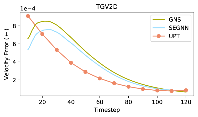
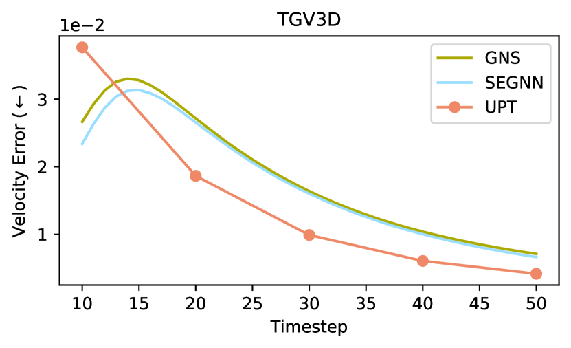
Model	Time	Speedup	Device
SPH	4.9s	1x	A6000
SEGNN	2.76s	2x	A100
GNS	0.56s	9x	A100
UPT	0.05s	98x	A100

Figure 8: (Top) Mean Euclidean norm of the velocity error over all particles for different timesteps. UPTs effectively learn the underlying field dynamics, resulting in lower velocity error as the trajectory evolves in time. (Bottom left) Visualization of the velocity field modeled by UPT (depicted in white) compared to the ground truth particle velocities. (Bottom right) Comparison of simulation/rollout runtimes for a TGV2D trajectory with 125 timesteps and 2500 particles across SPH simulation, GNS/SEGNN, and UPT, which has an inference time that results in a 98-fold speedup compared to SPH, a 55-fold speedup compared to SEGNN and a 11-fold speedup compared to GNS.

5 Conclusion

We have introduced Universal Physics Transformers (UPTs), a novel learning paradigm which models a wide range of spatio-temporal problems – both for Lagrangian and Eulerian discretization schemes. UPTs operate without grid- or particle-based latent structures, enabling flexibility across meshes and number of particles. The UPT training procedure separates responsibilities between components, allowing a forward propagation in time purely within the latent space. Finally, UPTs allow for queries of the latent space representation at any point in space-time.

Appendix A Computational fluid dynamics

This appendix discusses the Navier-Stokes equations and selected numerical integration schemes, which are related to the experiments presented in this paper. This is not an complete introduction into the field, but rather encompasses the concepts which are important to follow the experiments discussed in the main paper.

First, we discuss the different operators of the Navier-Stokes equations, relate compressible and incompressible formulations, and discuss why Navier-Stokes equations are difficult to solve. Second, we discuss turbulence as one of the fundamental challenges of computational fluid dynamics (CFD), explicitly working out the difference for two dimensional and three dimensional turbulence modeling. Third, we introduce Reynolds-averaged Navier-Stokes equations (RANS) as an numerical approach for steady-state turbulence modeling, and the SIMPLE and PISO algorithms as steady-state and transient solvers, respectively. Finally, we discuss Lagrangian discretization schemes, focusing on smoothed particle hydrodynamics (SPH).

A.1 Navier-Stokes equations

In our experiments, we mostly work with the imcompressible Navier-Stokes equations (Temam, 2001). In two spatial dimensions, the evolution equation of the velocity flow field $\bm{u}:[0,T]\times U\subset\mathbb{R}^{3}\rightarrow\mathbb{R}^{2}$, $\bm{u}(t,x,y)=(u_{1}(t,x,y),u_{2}(t,x,y))$ with internal pressure $\bm{p}(x,y)=(p_{1}(x,y),p_{2}(x,y))$ and external force field $\bm{f}(x,y)=(f_{1}(x,y),f_{2}(x,y))$ is given via:

$$\begin{split}\frac{\partial u_{1}}{\partial t}=&-u_{1}\frac{\partial u_{1}}{\partial x}-u_{2}\frac{\partial u_{1}}{\partial y}+\mu\left(\frac{\partial^{2}u_{1}}{\partial x^{2}}+\frac{\partial^{2}u_{1}}{\partial y^{2}}\right)-\frac{\partial p_{1}}{\partial x}+f_{1}\\ \frac{\partial u_{2}}{\partial t}=&-u_{1}\frac{\partial u_{2}}{\partial x}-u_{2}\frac{\partial u_{2}}{\partial y}+\mu\left(\frac{\partial^{2}u_{2}}{\partial x^{2}}+\frac{\partial^{2}u_{2}}{\partial y^{2}}\right)-\frac{\partial p_{2}}{\partial y}+f_{2}\\ 0=&\ \frac{\partial u_{1}}{\partial x}+\frac{\partial u_{2}}{\partial y}\end{split}$$ (3)

This system is usually written in a shorter and more convenient form:

$$\begin{split}\frac{\partial\bm{u}}{\partial t}&=-\bm{u}\cdot\nabla\bm{u}+\mu\nabla^{2}\bm{u}-\nabla p+\bm{f}\\ 0&=\nabla\cdot\bm{u}\ ,\end{split}$$ (4)

where

$$\bm{u}\cdot\nabla\bm{u}=\left(\begin{array}[]{cc}u_{1}&u_{2}\\ \end{array}\right)\cdot\left(\begin{array}[]{cc}\dfrac{\partial u_{1}}{\partial x}&\dfrac{\partial u_{2}}{\partial x}\\[8.61108pt] \dfrac{\partial u_{1}}{\partial y}&\dfrac{\partial u_{2}}{\partial y}\end{array}\right)$$ (8)

is called the convection, i.e., the rate of change of $\bm{u}$ along $\bm{u}$, and

$$\mu\nabla^{2}\bm{u}=\mu\left(\begin{array}[]{cc}\dfrac{\partial}{\partial x}&\dfrac{\partial}{\partial y}\\ \end{array}\right)\cdot\left(\begin{array}[]{c}\dfrac{\partial}{\partial x}\\[8.61108pt] \dfrac{\partial}{\partial y}\\ \end{array}\right)\left(\begin{array}[]{c}u_{1}\\ u_{2}\\ \end{array}\right)=\mu\left(\frac{\partial^{2}}{\partial x^{2}}+\frac{\partial^{2}}{\partial y^{2}}\right)\left(\begin{array}[]{c}u_{1}\\ u_{2}\\ \end{array}\right)\$$ (16)

the viscosity, i.e., the diffusion or net movement of $\bm{u}$ with viscosity parameter $\nu$. The constraint

$$\left(\begin{array}[]{cc}\dfrac{\partial}{\partial x}&\dfrac{\partial}{\partial y}\\ \end{array}\right)\cdot\left(\begin{array}[]{c}u_{1}\\ u_{2}\\ \end{array}\right)=\frac{\partial u_{1}}{\partial x}+\frac{\partial u_{2}}{\partial y}=0$$ (20)

yields mass conservation of the Navier-Stokes equations.

The incompressible version of the NS equations above are commonly used in the study of water flow, low-speed air flow, and other scenarios where density changes are negligible. Its compressible counterpart additionally accounts for variations in fluid density and temperature which is necessary to accurately model gases at high speeds (starting in the magnitude of speed of sound) or scenarios with significant changes in temperature. These additional considerations result in a more complex momentum and continuity equation.

Why are the Navier-Stokes equations difficult to solve? One major difficulty is that no equation explicitly models the unknown pressure field. Instead, the conservation of mass $\nabla\cdot\bm{u}=0$ is an implicit constraint on the velocity fields. Additionally, the nonlinear nature of the NS equations makes them notoriously harder to solve than parabolic or hyperbolic PDEs such as the heat or wave equation, respectively. Also, the occurrence of turbulence as discussed in the next subsection which is due to the fact that small and large scales are coupled such that small errors, can have a large effect on the computed solution.

Computational fluid dynamics (CFD) uses numerical schemes to discretize and solve fluid flows. CFD simulates the free-stream flow of the fluid, and the interaction of the fluid (liquids and gases) with surfaces defined by boundary conditions. As such, CFD comprises many challenging phenomena, such as interactions with boundaries, mixing of different fluids, transonic, i.e, coincident emergence of subsonic and supersonic airflow, or turbulent flows.

A.2 Turbulence

Turbulence (Pope, 2001; Mathieu & Scott, 2000) is one of the key aspects of CFD and refers to chaotic and irregular motion of fluid flows, such as air or water. It is characterized by unpredictable changes in velocity, pressure, and density within the fluid. Turbulent flow is distinguished from laminar flow, which is smooth and orderly. There are several factors that can contribute to the onset of turbulence, including high flow velocities, irregularities in the shape of surfaces over which the fluid flows, and changes in the fluid’s viscosity. Turbulence plays a significant role in many natural phenomena and engineering applications, influencing processes such as mixing, heat transfer, and the dispersion of particles in fluids. Understanding and predicting turbulence is crucial in fields like fluid dynamics, aerodynamics, and meteorology. Turbulent flows occur at high Reynolds numbers

$$\text{Re}=\frac{\rho\nu L}{\mu}\ ,$$ (21)

where $\rho$ is the density of the fluid, $\nu$ is the velocity of the fluid, $L$ is the linear dimension, e.g., the width of a pipe, and $\mu$ is the viscosity. Turbulent flows and are dominated by inertial forces, which tend to produce chaotic eddies, vortices and other flow instabilities.

Turbulence in 3D vs turbulence in 2D. For high Reynolds numbers, i.e., in the turbulent regime, solutions to incompressible Navier-Stokes equations differ in three dimensions compared to two dimensions by a phenomenon called energy cascade. Energy cascade orchestrates the transfer of kinetic energy from large-scale vortices to progressively smaller scales until it is eventually converted into thermal energy. In three dimensions, this energy cascade is responsible for to the continuous formation of vortex structures at various scales, and thus for the emergence of high-frequency features. In contrast to three dimensions, the energy cascade is inverted in two dimensions, i.e., energy is transported from smaller to larger scales, resulting in more homogeneous, long-lived structures. Mathematically the difference between three dimensional and two dimensional turbulence modeling can be best seen be rewriting the Navier-Stokes equations in vorticity formulation, where the vorticity ${\bm{\omega}}$ is the curl of the flow field, i.e., ${\bm{\omega}}=\nabla\times\bm{u}$, with $\times$ here denoting the cross product. This derivation can be found in many standard texts on Navier-Stokes equation , e.g. Tsai (2018, Section 1.4.), and for the reader’s convenience we briefly repeat the derivation here. We start using Eq. (4), setting $\bm{f}=0$ for simplicity:

$$\frac{\partial\bm{u}}{\partial t} =-\bm{u}\cdot\nabla\bm{u}+\mu\nabla^{2}\bm{u}-\nabla p$$ (22)

$$=-\nabla\left(\frac{1}{2}\bm{u}\cdot\bm{u}\right)+\bm{u}\times\nabla\times\bm{u}+\mu\nabla^{2}\bm{u}-\nabla p\ ,$$ (23)

where we applied the dot product rule for derivatives of vector fields:

$$\nabla\left(\frac{1}{2}\bm{u}\cdot\bm{u}\right)=\bm{u}\cdot\nabla\bm{u}+\bm{u}\times\nabla\times\bm{u}\ .$$ (24)

Next, we take the curl of the right and the left hand side:

$$\frac{\partial}{\partial t}\left(\nabla\times\bm{u}\right) =-\frac{1}{2}\underbrace{\nabla\times\nabla(\bm{u}\cdot\bm{u})}_{=0}+\nabla\times\bm{u}\times\nabla\times\bm{u}+\mu\nabla^{2}\left(\nabla\times\bm{u}\right)-\underbrace{\nabla\times\nabla p}_{=0}$$ (25)

$$\frac{\partial{\bm{\omega}}}{\partial t} =\nabla\times\left(\bm{u}\times{\bm{\omega}}\right)+\mu\nabla^{2}{\bm{\omega}}$$ (26)

using the property that the curl of a gradient is zero. Lastly, using that the divergence of the curl is again zero (i.e. $\nabla\cdot{\bm{\omega}}=0$), via the identity $\displaystyle\nabla\times\left(\bm{u}\times{\bm{\omega}}\right)=\left({\bm{\omega}}\cdot\nabla\right)\bm{u}-\left(\bm{u}\cdot\nabla\right){\bm{\omega}}+\bm{u}\underbrace{\nabla\cdot{\bm{\omega}}}_{=0}-{\bm{\omega}}\underbrace{\nabla\cdot\bm{u}}_{=0}$, we obtain:

$$\frac{\partial{\bm{\omega}}}{\partial t}+\left(\bm{u}\cdot\nabla\right){\bm{\omega}} =\left({\bm{\omega}}\cdot\nabla\right)\bm{u}+\mu\nabla^{2}{\bm{\omega}}$$ (27)

$$\frac{D{\bm{\omega}}}{Dt} =\left({\bm{\omega}}\cdot\nabla\right)\bm{u}+\mu\nabla^{2}{\bm{\omega}}\ ,$$ (28)

where $\displaystyle\frac{D{\bm{\omega}}}{Dt}=\frac{\partial{\bm{\omega}}}{\partial t}+\left(\bm{u}\cdot\nabla\right){\bm{\omega}}$.

For two dimensional flows

$$\bm{u}=\left(\begin{array}[]{c}u_{1}\\ u_{2}\\ 0\\ \end{array}\right)\ \text{and}\ \ {\bm{\omega}}=\nabla\times\bm{u}=\left(\begin{array}[]{c}0\\ 0\\ \frac{\partial u_{2}}{\partial x}-\frac{\partial u_{1}}{\partial y}\\ \end{array}\right)$$ (35)

and thus $\displaystyle\frac{\partial{\bm{\omega}}}{\partial t}=0$ in two dimensions. Consequently, the length of a vortex cannot change in two dimensions, resulting in homogeneous, long-lived structures. Conversely, in three dimensions,

$$\frac{D\omega_{i}}{Dt}=\underbrace{\omega_{j}\frac{\partial u_{i}}{\partial x_{j}}}_{\text{vortex turning and stretching}}+\underbrace{\mu\frac{\partial^{2}\omega_{i}}{\partial x_{j}\partial x_{j}}}_{\text{diffusion}}\ .$$ (36)

For example, picking an arbitrary component:

$$\frac{D\omega_{2}}{Dt}=\underbrace{\omega_{1}\frac{\partial u_{2}}{\partial x_{1}}}_{\text{vortex turning}}+\underbrace{\omega_{2}\frac{\partial u_{2}}{\partial x_{2}}}_{\text{vortex stretching}}+\underbrace{\omega_{3}\frac{\partial u_{2}}{\partial x_{3}}}_{\text{vortex turning}}+\underbrace{\mu\left(\frac{\partial^{2}\omega_{2}}{\partial x_{1}\partial x_{1}}+\ \frac{\partial^{2}\omega_{2}}{\partial x_{2}\partial x_{2}}+\frac{\partial^{2}\omega_{2}}{\partial x_{3}\partial x_{3}}\right)}_{\text{diffusion}}\ .$$ (37)

There’s been several approaches to model turbulence with the help of Deep Learning. Predominantly models for two dimensional scenarios have been suggested (Pfaff et al., 2020; Li et al., 2020a; Brandstetter et al., 2022c; Kochkov et al., 2021; Kohl et al., 2023). Due to the higher complexity (as discussed above) and memory- and compute costs comparably less work was done in the 3D case (Stachenfeld et al., 2022; Lienen et al., 2023).

A.3 Numerical modeling based on Eulerian discretization schemes

Various approaches are available for numerically addressing turbulence, with different schemes suited to different levels of computational intensity. Among these, Direct Numerical Simulation (DNS) (Moin & Mahesh, 1998) stands out as the most resource-intensive method, involving the direct solution of the unsteady Navier-Stokes equations.

DNS is renowned for its capability to resolve even the minutest eddies and time scales present in turbulent flows. While DNS does not necessitate additional closure equations, a significant drawback is its high computational demand. Achieving accurate solutions requires the utilization of very fine grids and extremely small time steps. This is based on Kolmoqorov (1941) and Kolmogorov (1962) which give the minimum spacial and temporal scales that need to be resolved for accurately simulating turbulence. The discretization-scales for both time and space needed for 3D-problems become very small and simulations computationally extremely expensive.

This computational intensity of DNS resulted in the development of turbulence modeling, with Large Eddy Simulations (LES) (Smagorinsky, 1963) and Reynolds-averaged Navier-Stokes equations (RANS) (Reynolds, 1895) being two prominent examples. LES aim to reduce computational cost by neglecting the computationally expensive smallest length scales in turbulent flows. This is achieved through a low-pass filtering of the Navier–Stokes equations, effectively removing fine-scale details via time- and spatial-averaging. In contrast, the Reynolds-averaged Navier–Stokes equations (RANS equations) are based on time-averaging. The foundational concept is Reynolds decomposition, attributed to Osborne Reynolds, where an instantaneous quantity is decomposed into its time-averaged and fluctuating components.

Turbulent scenarios where the fluid conditions change over time are an example of transient flows. These are typically harder to model/solve than steady state flows where the fluid properties exhibit only negligible changes over time.

In the following, we discuss Reynolds-averaged Navier-Stokes equations (RANS) as a numercial approach for steady-state turbulence modeling, and the SIMPLE and PISO algorithms as steady-state and transient numerical solvers, respectively.

A.3.1 Reynolds-averaged Navier-Stokes equations

Reynolds-averaged Navier-Stokes equations (RANS) are used to model time-averaged fluid properties such as velocity or pressure that result in a steady state which does not change over time. Writing  (4) in Einstein notation we get

$$\frac{\partial u_{i}}{\partial t}= -u_{j}\frac{\partial u_{i}}{\partial x_{j}}+\mu\frac{\partial^{2}u_{i}}{\partial x_{j}\partial x_{j}}-\frac{\partial p}{\partial x_{i}}+f_{i}$$

$$0= \ \frac{\partial u_{i}}{\partial x_{i}}\ .$$ (38)

Taking the Reynolds decomposition (Reynolds, 1895) $g(t,x_{1},x_{2}):=\bar{g}(x_{1},x_{2})+g^{\prime}(t,x_{1},x_{2})$ with $\bar{g}(x_{1},x_{2}):=\lim_{T\to\infty}1/T\int_{0}^{T}g(x_{1},x_{2},t)dt$ being the time-average on $[0,T]$ of a scalar valued function $g$, and splitting each term of both equations into it’s time-averaged and fluctuating part we get

$$\frac{\partial(\bar{u}_{i}+u^{\prime}_{i})}{\partial t}= -(\bar{u}_{j}+u^{\prime}_{j})\frac{\partial(\bar{u}_{i}+u^{\prime}_{i})}{\partial x_{j}}+\mu\frac{\partial^{2}(\bar{u}_{i}+u^{\prime}_{i})}{\partial x_{j}\partial x_{j}}-\frac{\partial(\bar{p}+p^{\prime})}{\partial x_{i}}+(\bar{f}_{i}+f^{\prime}_{i})$$

$$0= \ \frac{\partial(\bar{u}_{i}+u^{\prime}_{i})}{\partial x_{i}}.$$

Time-averaging these equations together with the property that the time-average of the fluctuating parts equals zero results in

$$\bar{u}_{j}\frac{\partial\bar{u}_{i}}{\partial x_{j}}+\overline{u^{\prime}_{j}\frac{\partial u^{\prime}_{i}}{\partial x_{j}}}= \mu\frac{\partial^{2}\bar{u}_{i}}{\partial x_{j}\partial x_{j}}-\frac{\partial\bar{p}}{\partial x_{i}}+\bar{f}_{i}$$ (39)

$$0= \ \frac{\partial\bar{u}_{i}}{\partial x_{i}}.$$

Using the the mass conserving equation (A.3.1) the momentum equation (39) can be rewritten as

$$\bar{u}_{j}\frac{\partial\bar{u}_{i}}{\partial x_{j}}= \bar{f}_{i}+\frac{\partial}{\partial x_{j}}\left[\mu\left(\frac{\partial\bar{u}_{i}}{\partial x_{j}}+\frac{\partial\bar{u}_{j}}{\partial x_{i}}\right)-\bar{p}\delta_{ij}-\overline{u^{\prime}_{i}u^{\prime}_{j}}\right]$$

where $-\overline{u^{\prime}_{i}u^{\prime}_{j}}$ is called the Reynolds stress which needs further modeling to solve the above equations. More specifically, this is referred to as the Closure Problem which led to many turbulence models such as $k\text{-}\epsilon$ (Hanjalic & Brian, 1972) or $k\text{-}\omega$ (Wilcox, 2008). Analogously the 3D RANS equations can be derived. This turbulence model consists of simplified equations that predict the statistical evolution of turbulent flows. Due to the Reynolds stress there still remain velocity fluctuations in the RANS equations. To get equations that contain only time-averaged quantities the RANS equations need to be closed by modeling the Reynolds stress as a function of the mean flow such that any reference to the fluctuating parts is removed. The first such approach led to the eddy viscosity model (Boussinesq, 1877) for 3-d incompressible Navier Stokes:

$$-\overline{u^{\prime}_{i}u^{\prime}_{j}}=\nu_{t}\left(\frac{\partial\bar{u}_{i}}{\partial x_{j}}+\frac{\partial\bar{u}_{j}}{\partial x_{i}}\right)-\frac{2}{3}k\delta_{ij}$$

with the turbulence eddy viscosity $\nu_{t}>0$ and the turbulence kinetic energy $k=1/2\ \overline{u^{\prime}_{i}u^{\prime}_{i}}$ based on Boussinesq’s hypothesis that turbulent shear stresses act in the same direction as shear stresses due to the averaged flow. The $k$-$\epsilon$ model employs Boussinesq’s hypothesis by using comparably low-cost computations for the eddy viscosity by means of two additional transport equations for turbulence kinetic energy $k$ and dissipation $\epsilon$

$$\frac{\partial(\rho k)}{\partial t}+\frac{\partial(\rho ku_{i})}{\partial x_{i}} =\frac{\partial}{\partial x_{j}}\left[\frac{\nu_{t}}{\sigma_{k}}\frac{\partial k}{\partial x_{j}}\right]+2\nu_{t}E_{ij}E_{ij}-\rho\epsilon$$

$$\frac{\partial(\rho\epsilon)}{\partial t}+\frac{\partial(\rho\epsilon u_{i})}{\partial x_{i}} =\frac{\partial}{\partial x_{j}}\left[\frac{\nu_{t}}{\sigma_{\epsilon}}\frac{\partial\epsilon}{\partial x_{j}}\right]+C_{1\epsilon}\frac{\epsilon}{k}2\nu_{t}E_{ij}E_{ij}-C_{2\epsilon}\rho\frac{\epsilon^{2}}{k}$$

with the rate of deformation $E_{ij}$, eddy viscosity $\nu_{t}=\rho C_{\nu}k^{2}/\epsilon$, and adjustable constants $C_{\nu},C_{1\epsilon},C_{2\epsilon},\sigma_{\epsilon},\sigma_{k}$. In our experiment section 4.1 solutions of simulations based on the RANS $k$-$\epsilon$ turbulence model are used as ground truth where the quantity of interest is the pressure field given the shape of a vehicle.

A.3.2 SIMPLE and PISO algorithm

Next, we introduce two popular algorithms that try to solve Eq. (4) numerically, where the main idea is to couple pressure and velocity computations. Specifically, we will discuss the SIMPLE (Semi-Implicit Method for Pressure-Linked Equations) (Patankar & Spalding, 1972) and PISO (Pressure Implicit with Splitting of Operators) (Issa, 1986) algorithm, which are implemented in OpenFOAM as well. The essence of these algorithms are the following four main steps:

1. In a first step, the momentum equation is discretized by using suitable finite volume discretizations of the involved derivatives. This leads to a linear system for $\bm{u}$ for a given pressure gradient $\nabla\bm{p}$:

   $$\mathcal{M}\bm{u}=-\nabla\bm{p}.$$ (40)

   However, this computed velocity field $\bm{u}$ does not yet satisfy the continuity equations $\nabla\cdot\bm{u}=0$.

2. In a next step, let us denote by $\mathcal{A}$ the diagonal part of $\mathcal{M}$ and introduce $\mathcal{H}$, so that

   $$\mathcal{H}=\mathcal{A}\bm{u}-\mathcal{M}\bm{u}.$$ (41)

   Taking into account $\mathcal{M}\bm{u}=-\nabla\bm{u}$ allows to easily rearrange Eq. (41) for $\bm{u}$, since $\mathcal{A}$ is easily invertible. This gives us:

   $$\bm{u}=\mathcal{A}^{-1}\mathcal{H}-\mathcal{A}^{-1}\nabla\bm{p}.$$ (42)

3. Now we substitute Eq. (42) into the continuity equation yielding

   $$\nabla\cdot(\mathcal{A}^{-1}\nabla\bm{p})=\nabla\cdot(\mathcal{A}^{-1}\mathcal{H}),$$ (43)

   which is a Poisson equation for the pressure $\bm{p}$ that can be solved again numerically.

4. This pressure field can now be used to correct the velocity field by again applying Eq. (42). This is the pressure-corrector stage and this $\bm{u}$ now satisfies the continuity equation. Now, however, the pressure equation is no longer valid, since $\mathcal{H}$ depends on $\bm{u}$ as well. A way out here is iterating these procedures, which is the main idea of the SIMPLE and PISO algorithm.

The SIMPLE algorithm just iterates steps 1-4 several times , which is then called an outer corrector loop. In contrast, the PISO algorithm solves the momentum predictor $\mathcal{M}\bm{u}=-\nabla\bm{p}$ (i.e. step 1) only once and then iterates steps 2-4, which then result in an inner loop. In both algorithms, in case the meshes are non orthogonal, step 3, i.e. solving the Poisson equation, can also be repeated several times before moving to step 4. For stability reasons, the SIMPLE algorithm is preferred for stationary equations (since it implicitly promotes under-relaxation), whereas in case of time-dependent flows, one usually considers the PISO algorithm (since in practice, for each timestep several thousands of iterations are usually required until convergence, which is computationally very expensive).

A.4 Lagrangian discretization schemes

In contrast to such grid- and mesh-based representations, in Lagrangian schemes, the discretization is carried out using finitely many material points, often referred to as particles, which move with the local deformation of the continuum. Roughly speaking, there are three families of Lagrangian schemes: discrete element methods (Cundall & Strack, 1979), material point methods (Sulsky et al., 1994; Brackbill & Ruppel, 1986), and smoothed particle hydrodynamics (SPH) (Gin, 1977; Lucy, 1977; Monaghan, 1992, 2005).

A.4.1 Smoothed particle hydrodynamics

The core idea behind SPH is to divide a fluid into a set of discrete moving elements referred to as particles. These particles interact through using truncated radial interpolation kernel functions with characteristic radius known as the smoothing length. The truncation is justified by the assumption of locality of interactions between particles which allows to approximate the properties of the fluid at any arbitrary location. For particle $i$ its position $\bm{x}_{i}$ is given by its velocity $u_{i}$ such that $\frac{\partial\bm{x}_{i}}{\partial t}=\bm{u}_{i}$. The modeling of particle interaction by kernel functions implies that physical properties of any particle can be obtained by aggregating the relevant properties of all particles within the range of the kernel. For example, the density $\rho_{i}$ of a particle can be expressed as $\rho(\bm{x}_{i})=\sum_{j}\rho_{j}V_{j}W(||\bm{x}_{i}-\bm{x}_{j}||,h)$ with $W$ being a kernel, $h$ its smoothing length, and $V_{j}$ the volumes of the respective particles. Rewriting the weakly-compressible Navier-Stokes equations with quantities as in (4) and additional Reynolds number Re and density $\rho$

$$\frac{\partial\bm{u}}{\partial t} =\frac{1}{\text{Re}}\nabla^{2}\bm{u}-\frac{1}{\rho}\nabla p+\frac{1}{\rho}\bm{f}$$

$$\frac{\partial\rho}{\partial t} =-\rho(\nabla\cdot\bm{u})$$

in terms of these kernel interpolations leads to a system of ordinary differential equations (ODEs) for the particle accelerations (Morris et al., 1997) where the respective velocities and positions can be computed by integration. One of the advantages of SPH compared to Eulerian discretization techniques is that SPH can handle large topological changes as no connectivity constraints between particles are required, and advection is treated exactly (Toshev et al., 2023a; Monaghan & Gingold, 1983). The lack of a mesh significantly simplifies the model implementation and opens up more possibilities for parallelization compared to Eulerian schemes (Harada et al., 2007; Crespo et al., 2011). However, for accurately resolving particle dynamics on small scales a large number of particles is needed to achieve a resolution comparable to grid-based methods specifically when the metric of interest is not directly related to density which makes SPH more expensive (Colagrossi & Maurizio, 2003). Also, setting boundary conditions such as inlets, outlets, and walls is more difficult than for grid-based methods.

Appendix B Experimental details

B.1 General

All experiments are conducted on A100 GPUs. All experiments linearly scale the learning rate with the batchsize, exclude normalization and bias parameters from the weight decay, follow a linear warmup $\rightarrow$ cosine decay learning rate schedule (Loshchilov & Hutter, 2017) and use the AdamW (Kingma & Ba, 2015; Loshchilov & Hutter, 2019) optimizer. Transformer blocks follow a standard pre-norm architecture as used in ViT (Dosovitskiy et al., 2020).

B.2 Feature modulation

We apply feature modulation to condition models to time/velocity. We use different forms of feature modulation in accordance with existing works depending on the model type. FiLM (Perez et al., 2018) is used for U-Net, the “Spatial-Spectral” conditioning of Gupta & Brandstetter (2022) is used for FNO based models and DiT (Li et al., 2022a) is used for transformer blocks. For perceiver blocks, we extend the modulation of DiT to seperately modulate queries from keys/values.

B.3 ShapeNet-Car

Dataset

We test on the dataset generated by Umetani & Bickel (2018), which consists 889 car shapes from ShapeNet (Chang et al., 2015) where side mirrors, spoilers and tires were removed. We randomly split the 889 simulations into 700 train and 189 test samples. Each sample consists of 3682 mesh points, including a small amount of points that are not part of the car mesh. We filter all points that do not belong to the car mesh, resulting in 3586 points per sample. For each point, we predict the associated pressure value. As there is no notion of time and the inflow velocity is constant, no feature modulation is necessary. We use the transformer positional encoding (Vaswani et al., 2017), and, therefore rescale all positions to the range [0, 200].

Baselines

As baselines we consider FNO, U-Net and GINO. For FNO, we use a hidden dimension of 64 and 16/24/24 Fourier modes per dimension, and train with a learning rate of 1e-3/1e-3/5e-4 for grid resolutions $32^{3}/48^{3}/64^{3}$, respectively. We also tried using 32 Fourier modes for a grid resolution of $64^{3}$, which performed worse than using 24 modes.

The U-Net baseline follows the architecture used as baseline in GINO which consists of 4 downsampling and 4 upsampling blocks where each block consists of two GroupNorm (Wu & He, 2018)$\rightarrow$Conv3d$\rightarrow$ReLU (Nair & Hinton, 2010) subblocks. The initial hidden dimension is set to 64 then doubled in each downsampling block and halved in each upsampling block. Similar to FNO, we considered a higher initial hidden dimension for grid resolution $64^{3}$ which performed worse.

For GINO, we create a positional embedding of mesh- and grid-positions which are then used as input to a 3 layer MLP with GELU (Hendrycks & Gimpel, 2016) non-linearities to create messages. Messages from mesh-positions within a radius of each grid-position are accumulated which serves as input to the FNO part of GINO. The FNO uses 64 hidden dimensions with 16/24/32 modes per dimension for grid resolutions $32^{3}/48^{3}/64^{3}$, respectively. The GINO decoder encodes the query positions and again uses a 3 layer MLP with GELU non-linearities to create messages. Each query position aggregates the messages from grid-points within a radius. The radius for message aggregation is set to $10$. When using SDF features, the SDF features are encoded via a 2 layer MLP to the same dimension as the hidden dimension, and added onto the positional encoding of each grid point.

Hyperparameters

We train for 1000 epochs with 50 warmup epochs, a batchsize of 32. We tune the learning rate and model size for each model and report the best test loss.

UPT architecture

Due to a relatively low number of mesh points (3682), we use only a single perceiver block with 64 learnable query tokens as encoder, followed by the standard UPT architecture (transformer blocks as approximator and another perceiver block as decoder).

When additionally using SDF features as input, the SDF features are encoded by a shallow ConvNeXt V2 (Woo et al., 2023) that processes the SDF features into 512 (8x8x8) tokens, which are concatenated to the perceiver tokens. To distinguish between the two token types, a learnable vector per type is added to each of the tokens.

As UPT operates on the mesh directly, we can augment the data by randomly dropping mesh points of the input. Therefore we randomly sample between 80% and 100% of the mesh points during training and evaluate with all mesh points when training without SDF features. The decoder still predicts the pressure for all mesh points by querying the latent space with each mesh position. We also tried randomly dropping mesh points for GINO where it degraded performance.

Interpolated models

We consider U-Net and FNO as baseline models. These models only take SDF features as input since both models are bound to a regular grid representation, which prevents using the mesh points directly. The output feature maps are linearly interpolated to each mesh point from which a shallow MLP predicts the pressure at each mesh point. In the setting where no SDF features are used, we assign each mesh point a constant value of 1 and linearly interpolate onto a grid.

ShapeNet-Car extended results.

Table 4 extends the results from the main paper with the additional resolution of $48^{3}$.

Model	SDF	#Tokens	MSE	Mem. [GB]
U-Net	0	$64^{3}$	6.13	1.3
FNO	0	$64^{3}$	4.04	3.8
GINO	0	$64^{3}$	2.34	19.8
UPT (ours)	0	64	2.31	0.6
U-Net	32	$32^{3}$	3.66	0.2
FNO	32	$32^{3}$	3.31	0.5
GINO	32	$32^{3}$	2.90	2.1
UPT (ours)	32	$8^{3}+1024$	2.35	2.7
U-Net	48	$48^{3}$	3.33	0.5
FNO	48	$48^{3}$	3.29	1.6
GINO	48	$48^{3}$	2.57	7.9
UPT (ours)	48	$8^{3}+1024$	2.25	2.7
U-Net	64	$64^{3}$	2.83	1.3
FNO	64	$64^{3}$	3.26	3.8
GINO	64	$64^{3}$	2.14	19.8
UPT (ours)	64	$8^{3}+1024$	2.24	2.7

Table 4: Normalized test MSE for ShapeNet-Car pressure prediction. The loss is multiplied by 100. Memory denotes the amount required for a forward and backward pass of a single sample. UPTs can model the dynamics with a fraction of latent tokens compared to other models.

B.4 Transient flows

Dataset

The dataset consists of 10.000 simulations which we split into 8.000 training simulations, 1.000 validation simulations and 1.000 test simulations. Each simulations has a length of 100 seconds with a $\Delta t$ of 1s. The trajectories are randomly generated 2D windtunnel simulations with 1-4 objects placed in the tunnel.

The dataset is converted to float16 precision to save storage. From all training samples, data statistics are extracted to normalize inputs to approximately mean 0 and standard deviation 1. In order to get robust statistics, the normalization parameters are calculated only from values within the inter-quartile range. As the Pytorch function to calculate quartiles is not supported to handle such a large amount of values, we assume that values follow a Gaussian distribution with mean and variance from the data, which allows us to infer the inter-quartile range from the Gaussian CDF.

Additionally, we convert the normalized values $\tilde{u}^{t}_{i,k}$ to log scale to avoid extreme outliers which can lead to training instabilities:

$$u^{t}_{i,k}=\mbox{sign}(\tilde{u}^{t}_{i,k})\cdot\log(1+|\tilde{u}^{t}_{i,k}|)\ ,$$ (44)

where all functions/operations are applied point-wise to the individual vector components. We apply the same log-scale conversion to the decoder output $\hat{u}^{t}_{i,k}$.

Model scaling

We scale models by scaling the dimension of the model. For grid-based methods, we choose 64x64 as grid size which results in similar compute costs of GINO and UPT. As encoder and decoder operate on the mesh — which is more expensive than operating in the latent space — we use half of the approximator hidden dimension as hidden dimension for encoder and decoder. For example, for UPT-68M, we use hidden dimension 384 for the approximator and 192 for encoder/decoder. The hidden dimensions of the approximator are as follows: 128 for UPT-8M, 192 for UPT-17M and 384 for UPT-68M.

For UPT, we use 12 transformer blocks in total, which we distribute evenly across encoder, approximator and decoder (i.e. 4 transformer blocks for each component). As the decoder directly follows the approximator, this implementation detail only matters when training with inverse encoding and decoding to enable a latent rollout. In this setting, the decoder needs more expressive power than a single perceiver layer to decouple the latent propagation and the inverse encoding and decoding.

For GINO, we use 10/12/16 Fourier modes per dimension with a hidden dimension of 40/50/76 for the 8M/17M/68M parameter models, respectively. The hidden dimension of the encoder/decoder are the same ones as used for the UPT models.

For U-Nets, we use the Unet${}_{\text{mod}}$ architecture from Gupta & Brandstetter (2022) where we adjust the number of hidden dimensions to be approximately equal to the desired parameter counts. We use hidden dimensions 13/21/42 for the 8M/17M/68M parameter models, respectively.

Implementation

To efficiently use multi-GPU setups, we sample the same number of mesh points for each GPU. Without this modification, the FLOPS in the encoder would fluctuate drastically per GPU, which results in “busy waiting” time for GPUs with less FLOPS in the encoder. We also keep the number of mesh points constant between batches to avoid memory fluctuations, which allows using a larger batchsize. We rescale the x positions from the range $[-0.5,0.5]$ to $[0,200]$ and the y positions from $[-0.5,1]$ to $[0,300]$. We do this to avoid complications with the positional embedding (Vaswani et al., 2017) which was designed for positive integer positions. To create a graph out of mesh points, we use a radius graph with $r=5$ and limit the maximum number of graph edges per node to 32 to avoid memory fluctuations. We choose $r=5$ as it covers the whole domain when using a grid resolution of $64^{2}$.

Training

We train all models for 100 epochs using a batchsize of 1024 where we use gradient accumulation if the full batchsize does not fit into memory. Following common practices, we use AdamW (Kingma & Ba, 2015; Loshchilov & Hutter, 2019) for U-Net, FNO and GINO. As we encountered training instabilities when training UPTs on this dataset, we change the optimizer for UPTs to Lion (Chen et al., 2023). These instabilities manifest in sudden loss spikes from which the model can not recover. Using the Lion optimizer together with float32 precision training solves these instabilities in our experiments. When training with Lion, we use a learning rate of $5\times 10^{-5}$ and $1\times 10^{-4}$ otherwise. We also use float32 for GINO as we found that this improves performance. U-Net and FNO do not benefit from float32 and are therefore trained in bfloat16 precision.

We find float32 precision to be beneficial for GINO and UPTs, which is likely due to positional embeddings being too inaccurate with bfloat16 precision. Training with float16 instead of bfloat16 (to preserve the precision of the positional embedding while speeding up training) resulted in NaN values due to overflows. Therefore, we train all GINO and UPT models with float32.

Interpolated models

We train U-Net and FNO models as baseline on this task. To project the mesh onto a regular grid, we use a $k$-NN interpolation which takes the $k$ nearest neighbors of a grid position and interpolates between the values of the nerarest neighbors. Going from the grid back to the mesh is implemented via the grid_sample function of pytorch. For FNO, we use the same dimensions as in latent model of GINO and for U-Net, we scale the latent dimensions such that the model is in the same parameter count range as the other models.

Extended results

We show more qualitative results of the UPT-68M model in Fig. 9.

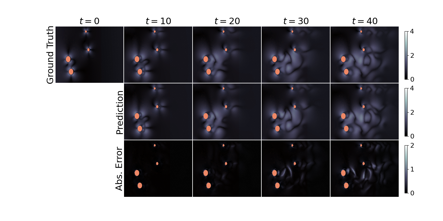
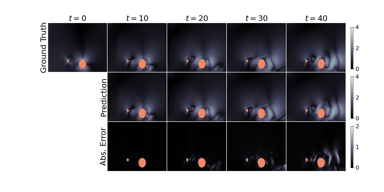
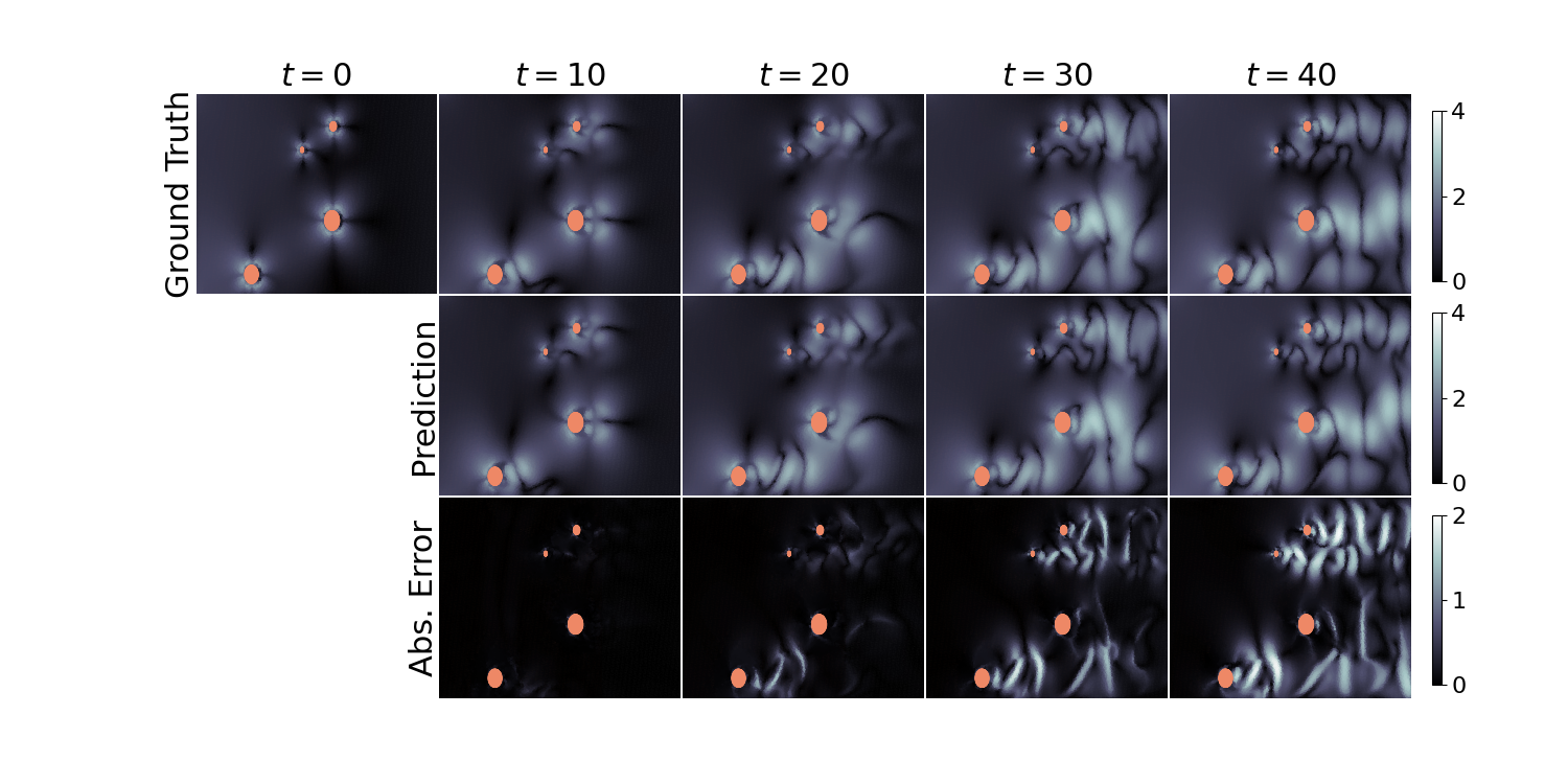
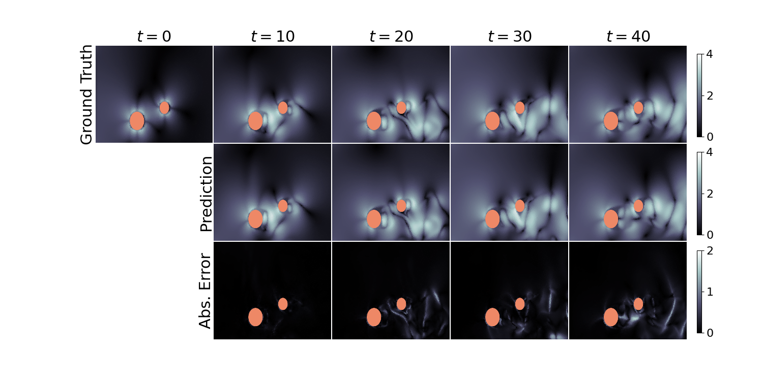
Figure 9: Exemplary visualizations of rollouts for transient flow simulations. Best viewed zoomed in.

B.5 Lagrangian fluid mechanics

Datasets

We use the Taylor-Green vortex datasets from Toshev et al. (2023b) for our Lagrangian experiments, comprising two dimensions (TGV2D) and three dimensions (TGV3D). The Taylor-Green vortex problem is characterized by a distinctive initial velocity field without an external driving force, resulting in a static decrease in kinetic energy over time. The TGV2D dataset includes 2500 particles, a sequence length of 126, and is characterized by a Reynolds number (Re) of 100. The data is split into 100/50/50 for training, validation, and testing, respectively. The TGV3D dataset consists of 8000 particles, a sequence length of 61, and a Reynolds number of 50. The data is partitioned into 200/100/100 for training, validation, and testing, respectively.

Baselines

The Graph Network-based Simulator (GNS) model (Sanchez-Gonzalez et al., 2020) is a popular learned surrogate for physical particle-based simulations. The architecture is kept simple, adhering to the encoder-processor-decoder principle (Battaglia et al., 2018), where the processor consists of multiple graph network blocks (Battaglia et al., 2016). The Steerable E(3)-equivariant Graph Neural Network (SEGNN) architecture (Brandstetter et al., 2022c) is a general implementation of an E($3$) equivariant GNN, where layers are directly conditioned on steerable attributes for both nodes and edges. The main building blocks are steerable MLPs, i.e., stacks of learnable linear Clebsch-Gordan tensor products interleaved with gated non-linearities (Weiler et al., 2018). SEGNN layers are message-passing layers (Gilmer et al., 2017) where steerable MLPs replace the traditional non-equivariant MLPs for both message and node update functions.

We utilize the checkpoints provided by Toshev et al. (2023b) for the comparisons in 4.3. Both GNS and SEGNN baseline models comprise 10 layers with latent dimensions of 128 and 64, respectively. The maximum irreps order of SEGNN are $l=1$, for more details see Toshev et al. (2023b).

Hyperparameters

We train using a batchsize of 128 for 50 epochs with a warmup phase of 10 epochs. We sample inputs between $50\%$ to $100\%$ of total particles. For optimization, we use AdamW (Loshchilov & Hutter, 2019) for all experiments with learning rate $10^{-3}$ and weight decay of $0.05$.

UPT architecture

For the TGV2D and TGV3D experiments, we use $n_{\text{s}}=256$ and $n_{\text{s}}=512$ supernodes, respectively. For TGV3D more supernodes are required due to the increased number of particles. Message passing is done with a maximum of four input points per supernode.

The encoder comprises four transformer blocks with a latent dimension of 96 and two attention heads. The encoder perceiver expands the latent dimension to 192 and outputs 128 latent tokens, using 128 learned queries and three attention heads. The approximator comprises four transformer blocks with a latent dimension of 192 and three attention heads. The decoder perceiver comprises again three attention heads. Overall, the parameter count of UPT amounts to 12.6M parameters.

References

- Gin (1977) Smoothed particle hydrodynamics: theory and application to non-spherical stars. Monthly notices of the royal astronomical society, 181(3):375–389, 1977.
- Andrychowicz et al. (2023) Andrychowicz, M., Espeholt, L., Li, D., Merchant, S., Merose, A., Zyda, F., Agrawal, S., and Kalchbrenner, N. Deep learning for day forecasts from sparse observations. arXiv preprint arXiv:2306.06079, 2023.
- Bartels (2016) Bartels, S. Numerical Approximation of Partial Differential Equations. Springer, 2016.
- Batatia et al. (2022) Batatia, I., Kovacs, D. P., Simm, G., Ortner, C., and Csányi, G. Mace: Higher order equivariant message passing neural networks for fast and accurate force fields. Advances in Neural Information Processing Systems, 35:11423–11436, 2022.
- Battaglia et al. (2016) Battaglia, P., Pascanu, R., Lai, M., Jimenez Rezende, D., et al. Interaction networks for learning about objects, relations and physics. Advances in neural information processing systems, 29, 2016.
- Battaglia et al. (2018) Battaglia, P. W., Hamrick, J. B., Bapst, V., Sanchez-Gonzalez, A., Zambaldi, V., Malinowski, M., Tacchetti, A., Raposo, D., Santoro, A., Faulkner, R., et al. Relational inductive biases, deep learning, and graph networks. arXiv preprint arXiv:1806.01261, 2018.
- Batzner et al. (2022) Batzner, S., Musaelian, A., Sun, L., Geiger, M., Mailoa, J. P., Kornbluth, M., Molinari, N., Smidt, T. E., and Kozinsky, B. E (3)-equivariant graph neural networks for data-efficient and accurate interatomic potentials. Nature communications, 13(1):2453, 2022.
- Bi et al. (2022) Bi, K., Xie, L., Zhang, H., Chen, X., Gu, X., and Tian, Q. Pangu-weather: A 3d high-resolution model for fast and accurate global weather forecast. arXiv preprint arXiv:2211.02556, 2022.
- Boussinesq (1877) Boussinesq, J. V. Essai sur la théorie des eaux courantes. Mémoires présentés par divers savants à l’Académie des Sciences, 23, 1877.
- Brackbill & Ruppel (1986) Brackbill, J. U. and Ruppel, H. M. Flip: A method for adaptively zoned, particle-in-cell calculations of fluid flows in two dimensions. Journal of Computational physics, 65(2):314–343, 1986.
- Brandstetter et al. (2022a) Brandstetter, J., Berg, R. v. d., Welling, M., and Gupta, J. K. Clifford neural layers for pde modeling. arXiv preprint arXiv:2209.04934, 2022a.
- Brandstetter et al. (2022b) Brandstetter, J., Hesselink, R., van der Pol, E., Bekkers, E. J., and Welling, M. Geometric and physical quantities improve e(3) equivariant message passing. In International Conference on Learning Representations, 2022b.
- Brandstetter et al. (2022c) Brandstetter, J., Worrall, D., and Welling, M. Message passing neural pde solvers. arXiv preprint arXiv:2202.03376, 2022c.
- Bryutkin et al. (2024) Bryutkin, A., Huang, J., Deng, Z., Yang, G., Schönlieb, C.-B., and Aviles-Rivero, A. Hamlet: Graph transformer neural operator for partial differential equations. arXiv preprint arXiv:2402.03541, 2024.
- Cao (2021) Cao, S. Choose a transformer: Fourier or galerkin. Advances in neural information processing systems, 34:24924–24940, 2021.
- Carey et al. (2024) Carey, N., Zanisi, L., Pamela, S., Gopakumar, V., Omotani, J., Buchanan, J., and Brandstetter, J. Data efficiency and long term prediction capabilities for neural operator surrogate models of core and edge plasma codes. arXiv preprint arXiv:2402.08561, 2024.
- Chang et al. (2015) Chang, A. X., Funkhouser, T. A., Guibas, L. J., Hanrahan, P., Huang, Q., Li, Z., Savarese, S., Savva, M., Song, S., Su, H., Xiao, J., Yi, L., and Yu, F. Shapenet: An information-rich 3d model repository. CoRR, abs/1512.03012, 2015.
- Chen et al. (2023) Chen, X., Liang, C., Huang, D., Real, E., Wang, K., Liu, Y., Pham, H., Dong, X., Luong, T., Hsieh, C., Lu, Y., and Le, Q. V. Symbolic discovery of optimization algorithms. CoRR, abs/2302.06675, 2023.
- Colagrossi & Maurizio (2003) Colagrossi, A. and Maurizio, L. Numerical simulation of interfacial flows by smoothed particle hydrodynamics. Journal of Computational Physics, 191, 2003.
- Crespo et al. (2011) Crespo, A., Dominguez, J. M., Barreiro, A., Gomez-Gasteira, M., and D, R. B. Gpus, a new tool of acceleration in cfd: efficiency and reliability on smoothed particle hydrodynamics methods. PLOS ONE, 6, 2011.
- Cundall & Strack (1979) Cundall, P. A. and Strack, O. D. A discrete numerical model for granular assemblies. geotechnique, 29(1):47–65, 1979.
- Dosovitskiy et al. (2020) Dosovitskiy, A., Beyer, L., Kolesnikov, A., Weissenborn, D., Zhai, X., Unterthiner, T., Dehghani, M., Minderer, M., Heigold, G., Gelly, S., et al. An image is worth 16x16 words: Transformers for image recognition at scale. arXiv preprint arXiv:2010.11929, 2020.
- Gilmer et al. (2017) Gilmer, J., Schoenholz, S. S., Riley, P. F., Vinyals, O., and Dahl, G. E. Neural message passing for quantum chemistry. In International conference on machine learning, pp. 1263–1272. PMLR, 2017.
- Guo et al. (2016) Guo, X., Li, W., and Iorio, F. Convolutional neural networks for steady flow approximation. In Proceedings of the 22nd ACM SIGKDD international conference on knowledge discovery and data mining, pp. 481–490, 2016.
- Gupta & Brandstetter (2022) Gupta, J. K. and Brandstetter, J. Towards multi-spatiotemporal-scale generalized pde modeling. arXiv preprint arXiv:2209.15616, 2022.
- Hanjalic & Brian (1972) Hanjalic, K. and Brian, L. A reynolds stress model of turbulence and its application to thin shear flows. Journal of Fluid Mechanics, 52(4):609–638, 1972.
- Hao et al. (2023) Hao, Z., Wang, Z., Su, H., Ying, C., Dong, Y., Liu, S., Cheng, Z., Song, J., and Zhu, J. Gnot: A general neural operator transformer for operator learning. In International Conference on Machine Learning, pp. 12556–12569. PMLR, 2023.
- Harada et al. (2007) Harada, T., Koshizuka, S., and Kawaguchi, Y. Smoothed particle hydrodynamics on gpus. Computer Graphics International, pp. 63–70, 2007.
- Hendrycks & Gimpel (2016) Hendrycks, D. and Gimpel, K. Gaussian error linear units (gelus). arXiv preprint arXiv:1606.08415, 2016.
- Issa (1986) Issa, R. Solution of the implicitly discretized fluid flow equations by operator-splitting. Journal of Computational Physics, 62, 1986.
- Jaegle et al. (2021a) Jaegle, A., Borgeaud, S., Alayrac, J.-B., Doersch, C., Ionescu, C., Ding, D., Koppula, S., Zoran, D., Brock, A., Shelhamer, E., et al. Perceiver io: A general architecture for structured inputs & outputs. In International Conference on Learning Representations, 2021a.
- Jaegle et al. (2021b) Jaegle, A., Gimeno, F., Brock, A., Vinyals, O., Zisserman, A., and Carreira, J. Perceiver: General perception with iterative attention. In International conference on machine learning, pp. 4651–4664. PMLR, 2021b.
- Kingma & Ba (2015) Kingma, D. P. and Ba, J. Adam: A method for stochastic optimization. In Bengio, Y. and LeCun, Y. (eds.), 3rd International Conference on Learning Representations, ICLR 2015, San Diego, CA, USA, May 7-9, 2015, Conference Track Proceedings, 2015.
- Kipf & Welling (2017) Kipf, T. N. and Welling, M. Semi-supervised classification with graph convolutional networks. In International Conference on Learning Representations, 2017.
- Kochkov et al. (2021) Kochkov, D., Smith, J. A., Alieva, A., Wang, Q., Brenner, M. P., and Hoyer, S. Machine learning–accelerated computational fluid dynamics. Proceedings of the National Academy of Sciences, 118(21):e2101784118, 2021.
- Kohl et al. (2023) Kohl, G., Chen, L.-W., and Thuerey, N. Turbulent flow simulation using autoregressive conditional diffusion models. arXiv preprint arXiv:2309.01745, 2023.
- Kolmogorov (1962) Kolmogorov, A. N. A refinement of previous hypotheses concerning the local structure of turbulence in a viscous incompressible fluid at high reynolds number. Journal of Fluid Mechanics, 13(1):82–85, 1962.
- Kolmoqorov (1941) Kolmoqorov, A. Local structure of turbulence in an incompressible fluid at very high reynolds numbers. CR Ad. Sei. UUSR, 30:305, 1941.
- Kovachki et al. (2021) Kovachki, N., Li, Z., Liu, B., Azizzadenesheli, K., Bhattacharya, K., Stuart, A., and Anandkumar, A. Neural operator: Learning maps between function spaces. arXiv preprint arXiv:2108.08481, 2021.
- Lam et al. (2022) Lam, R., Sanchez-Gonzalez, A., Willson, M., Wirnsberger, P., Fortunato, M., Pritzel, A., Ravuri, S., Ewalds, T., Alet, F., Eaton-Rosen, Z., et al. Graphcast: Learning skillful medium-range global weather forecasting. arXiv preprint arXiv:2212.12794, 2022.
- Lee & Carlberg (2021) Lee, K. and Carlberg, K. T. Deep conservation: A latent-dynamics model for exact satisfaction of physical conservation laws. In Proceedings of the AAAI Conference on Artificial Intelligence, volume 35, pp. 277–285, 2021.
- Li et al. (2022a) Li, J., Xu, Y., Lv, T., Cui, L., Zhang, C., and Wei, F. Dit: Self-supervised pre-training for document image transformer. In Magalhães, J., Bimbo, A. D., Satoh, S., Sebe, N., Alameda-Pineda, X., Jin, Q., Oria, V., and Toni, L. (eds.), MM ’22: The 30th ACM International Conference on Multimedia, Lisboa, Portugal, October 10 - 14, 2022, pp. 3530–3539. ACM, 2022a.
- Li et al. (2020a) Li, Z., Kovachki, N., Azizzadenesheli, K., Liu, B., Bhattacharya, K., Stuart, A., and Anandkumar, A. Fourier neural operator for parametric partial differential equations. arXiv preprint arXiv:2010.08895, 2020a.
- Li et al. (2020b) Li, Z., Kovachki, N., Azizzadenesheli, K., Liu, B., Bhattacharya, K., Stuart, A., and Anandkumar, A. Neural operator: Graph kernel network for partial differential equations. arXiv preprint arXiv:2003.03485, 2020b.
- Li et al. (2022b) Li, Z., Meidani, K., and Farimani, A. B. Transformer for partial differential equations’ operator learning. arXiv preprint arXiv:2205.13671, 2022b.
- Li et al. (2023) Li, Z., Kovachki, N. B., Choy, C., Li, B., Kossaifi, J., Otta, S. P., Nabian, M. A., Stadler, M., Hundt, C., Azizzadenesheli, K., et al. Geometry-informed neural operator for large-scale 3d pdes. arXiv preprint arXiv:2309.00583, 2023.
- Lienen et al. (2023) Lienen, M., Hansen-Palmus, J., Lüdke, D., and Günnemann, S. Generative diffusion for 3d turbulent flows. arXiv preprint arXiv:2306.01776, 2023.
- Lippe et al. (2023) Lippe, P., Veeling, B. S., Perdikaris, P., Turner, R. E., and Brandstetter, J. Pde-refiner: Achieving accurate long rollouts with neural pde solvers. arXiv preprint arXiv:2308.05732, 2023.
- Loshchilov & Hutter (2017) Loshchilov, I. and Hutter, F. SGDR: stochastic gradient descent with warm restarts. In 5th International Conference on Learning Representations, ICLR 2017, Toulon, France, April 24-26, 2017, Conference Track Proceedings. OpenReview.net, 2017.
- Loshchilov & Hutter (2019) Loshchilov, I. and Hutter, F. Decoupled weight decay regularization. In 7th International Conference on Learning Representations, ICLR 2019, New Orleans, LA, USA, May 6-9, 2019. OpenReview.net, 2019.
- Lu et al. (2019) Lu, L., Jin, P., and Karniadakis, G. E. Deeponet: Learning nonlinear operators for identifying differential equations based on the universal approximation theorem of operators. arXiv preprint arXiv:1910.03193, 2019.
- Lu et al. (2021) Lu, L., Jin, P., Pang, G., Zhang, Z., and Karniadakis, G. E. Learning nonlinear operators via deeponet based on the universal approximation theorem of operators. Nature machine intelligence, 3(3):218–229, 2021.
- Lucy (1977) Lucy, L. B. A numerical approach to the testing of the fission hypothesis. Astronomical Journal, vol. 82, Dec. 1977, p. 1013-1024., 82:1013–1024, 1977.
- Lusch et al. (2018) Lusch, B., Kutz, J. N., and Brunton, S. L. Deep learning for universal linear embeddings of nonlinear dynamics. Nature communications, 9(1):4950, 2018.
- Mathieu & Scott (2000) Mathieu, J. and Scott, J. An introduction to turbulent flow. Cambridge University Press, 2000.
- Mayr et al. (2023) Mayr, A., Lehner, S., Mayrhofer, A., Kloss, C., Hochreiter, S., and Brandstetter, J. Boundary graph neural networks for 3d simulations. In Proceedings of the AAAI Conference on Artificial Intelligence, volume 37, pp. 9099–9107, 2023.
- McCabe et al. (2023) McCabe, M., Blancard, B. R.-S., Parker, L. H., Ohana, R., Cranmer, M., Bietti, A., Eickenberg, M., Golkar, S., Krawezik, G., Lanusse, F., et al. Multiple physics pretraining for physical surrogate models. arXiv preprint arXiv:2310.02994, 2023.
- Merchant et al. (2023) Merchant, A., Batzner, S., Schoenholz, S. S., Aykol, M., Cheon, G., and Cubuk, E. D. Scaling deep learning for materials discovery. Nature, pp. 1–6, 2023.
- Moin & Mahesh (1998) Moin, P. and Mahesh, K. Direct numerical simulation: a tool in turbulence research. Annual review of fluid mechanics, 30(1):539–578, 1998.
- Monaghan (1992) Monaghan, J. J. Smoothed particle hydrodynamics. Annual review of astronomy and astrophysics, 30(1):543–574, 1992.
- Monaghan (2005) Monaghan, J. J. Smoothed particle hydrodynamics. Reports on progress in physics, 68(8):1703, 2005.
- Monaghan & Gingold (1983) Monaghan, J. J. and Gingold, R. A. Shock simulation by the particle method sph. Journal of computational physics, 52(2):374–389, 1983.
- Morris et al. (1997) Morris, J., Fox, P., and Zhu, Y. Modeling low reynolds number incompressible flows using sph. Journal of Computational Physics, 136, 1997.
- Morton et al. (2018) Morton, J., Jameson, A., Kochenderfer, M. J., and Witherden, F. Deep dynamical modeling and control of unsteady fluid flows. Advances in Neural Information Processing Systems, 31, 2018.
- Nair & Hinton (2010) Nair, V. and Hinton, G. E. Rectified linear units improve restricted boltzmann machines. In ICML, pp. 807–814. Omnipress, 2010.
- Nguyen et al. (2023) Nguyen, T., Brandstetter, J., Kapoor, A., Gupta, J. K., and Grover, A. Climax: A foundation model for weather and climate. arXiv preprint arXiv:2301.10343, 2023.
- Olver (2014) Olver, P. J. Introduction to partial differential equations. Springer, 2014.
- Patankar & Spalding (1972) Patankar, S. V. and Spalding, B. D. A calculation procedure for heat, mass and momentum transfer in three-dimensional parabolic flows. Int. J. of Heat and Mass Transfer, 15, 1972.
- Perez et al. (2018) Perez, E., Strub, F., de Vries, H., Dumoulin, V., and Courville, A. C. Film: Visual reasoning with a general conditioning layer. pp. 3942–3951. AAAI Press, 2018.
- Pfaff et al. (2020) Pfaff, T., Fortunato, M., Sanchez-Gonzalez, A., and Battaglia, P. W. Learning mesh-based simulation with graph networks. arXiv preprint arXiv:2010.03409, 2020.
- Pope (2001) Pope, S. B. Turbulent flows. Measurement Science and Technology, 12(11):2020–2021, 2001.
- Raonić et al. (2023) Raonić, B., Molinaro, R., Rohner, T., Mishra, S., and de Bezenac, E. Convolutional neural operators. arXiv preprint arXiv:2302.01178, 2023.
- Reynolds (1895) Reynolds, O. Iv. on the dynamical theory of incompressible viscous fluids and the determination of the criterion. Philosophical transactions of the royal society of london.(a.), (186):123–164, 1895.
- Rombach et al. (2022) Rombach, R., Blattmann, A., Lorenz, D., Esser, P., and Ommer, B. High-resolution image synthesis with latent diffusion models. In CVPR, pp. 10674–10685. IEEE, 2022.
- Ronneberger et al. (2015) Ronneberger, O., Fischer, P., and Brox, T. U-net: Convolutional networks for biomedical image segmentation. In MICCAI (3), volume 9351 of Lecture Notes in Computer Science, pp. 234–241. Springer, 2015.
- Sanchez-Gonzalez et al. (2020) Sanchez-Gonzalez, A., Godwin, J., Pfaff, T., Ying, R., Leskovec, J., and Battaglia, P. Learning to simulate complex physics with graph networks. In International conference on machine learning, pp. 8459–8468. PMLR, 2020.
- Scarselli et al. (2008) Scarselli, F., Gori, M., Tsoi, A. C., Hagenbuchner, M., and Monfardini, G. The graph neural network model. IEEE transactions on neural networks, 20(1):61–80, 2008.
- Seidman et al. (2022) Seidman, J., Kissas, G., Perdikaris, P., and Pappas, G. J. Nomad: Nonlinear manifold decoders for operator learning. Advances in Neural Information Processing Systems, 35:5601–5613, 2022.
- Smagorinsky (1963) Smagorinsky, J. General circulation experiments with the primitive equations: I. the basic experiment. Monthly weather review, 91(3):99–164, 1963.
- Stachenfeld et al. (2022) Stachenfeld, K., Fielding, D. B., Kochkov, D., Cranmer, M., Pfaff, T., Godwin, J., Cui, C., Ho, S., Battaglia, P., and Sanchez-Gonzalez, A. Learned simulators for turbulence. In International Conference on Learning Representations, 2022.
- Sulsky et al. (1994) Sulsky, D., Chen, Z., and Schreyer, H. L. A particle method for history-dependent materials. Computer methods in applied mechanics and engineering, 118(1-2):179–196, 1994.
- Takamoto et al. (2022) Takamoto, M., Praditia, T., Leiteritz, R., MacKinlay, D., Alesiani, F., Pflüger, D., and Niepert, M. Pdebench: An extensive benchmark for scientific machine learning. Advances in Neural Information Processing Systems, 35:1596–1611, 2022.
- Taylor & Green (1937) Taylor, G. I. and Green, A. E. Mechanism of the production of small eddies from large ones. Proceedings of the Royal Society of London. Series A-Mathematical and Physical Sciences, 158(895):499–521, 1937.
- Temam (2001) Temam, R. Navier-Stokes equations: theory and numerical analysis, volume 343. American Mathematical Soc., 2001.
- Thuerey et al. (2021) Thuerey, N., Holl, P., Mueller, M., Schnell, P., Trost, F., and Um, K. Physics-based deep learning. arXiv preprint arXiv:2109.05237, 2021.
- Toshev et al. (2023a) Toshev, A. P., Galletti, G., Brandstetter, J., Adami, S., and Adams, N. A. Learning lagrangian fluid mechanics with e ()-equivariant graph neural networks. arXiv preprint arXiv:2305.15603, 2023a.
- Toshev et al. (2023b) Toshev, A. P., Galletti, G., Fritz, F., Adami, S., and Adams, N. A. Lagrangebench: A lagrangian fluid mechanics benchmarking suite. In 37th Conference on Neural Information Processing Systems (NeurIPS 2023) Track on Datasets and Benchmarks, 2023b.
- Toshev et al. (2024) Toshev, A. P., Erbesdobler, J. A., Adams, N. A., and Brandstetter, J. Neural sph: Improved neural modeling of lagrangian fluid dynamics. arXiv preprint arXiv:2402.06275, 2024.
- Tsai (2018) Tsai, T.-P. Lectures on Navier-Stokes equations, volume 192. American Mathematical Soc., 2018.
- Umetani & Bickel (2018) Umetani, N. and Bickel, B. Learning three-dimensional flow for interactive aerodynamic design. ACM Trans. Graph., 37(4):89, 2018.
- Vaswani et al. (2017) Vaswani, A., Shazeer, N., Parmar, N., Uszkoreit, J., Jones, L., Gomez, A. N., Kaiser, Ł., and Polosukhin, I. Attention is all you need. Advances in neural information processing systems, 30, 2017.
- Vinuesa & Brunton (2022) Vinuesa, R. and Brunton, S. L. Enhancing computational fluid dynamics with machine learning. Nature Computational Science, 2(6):358–366, 2022.
- Weiler et al. (2018) Weiler, M., Geiger, M., Welling, M., Boomsma, W., and Cohen, T. S. 3d steerable cnns: Learning rotationally equivariant features in volumetric data. Advances in Neural Information Processing Systems, 31, 2018.
- Weller et al. (1998) Weller, H. G., Tabor, G., Jasak, H., and Fureby, C. A tensorial approach to computational continuum mechanics using object-oriented techniques. Computers in physics, 12(6):620–631, 1998.
- Wiewel et al. (2019) Wiewel, S., Becher, M., and Thuerey, N. Latent space physics: Towards learning the temporal evolution of fluid flow. In Computer graphics forum, volume 38, pp. 71–82. Wiley Online Library, 2019.
- Wilcox (2008) Wilcox, D. Formulation of the k-omega turbulence model revisited. AIAA Journal, 46(11):2823–2838, 2008.
- Woo et al. (2023) Woo, S., Debnath, S., Hu, R., Chen, X., Liu, Z., Kweon, I. S., and Xie, S. Convnext V2: co-designing and scaling convnets with masked autoencoders. In IEEE/CVF Conference on Computer Vision and Pattern Recognition, CVPR 2023, Vancouver, BC, Canada, June 17-24, 2023, pp. 16133–16142. IEEE, 2023.
- Wu et al. (2024) Wu, H., Luo, H., Wang, H., Wang, J., and Long, M. Transolver: A fast transformer solver for pdes on general geometries. arXiv preprint arXiv:2402.02366, 2024.
- Wu & He (2018) Wu, Y. and He, K. Group normalization. In ECCV (13), volume 11217 of Lecture Notes in Computer Science, pp. 3–19. Springer, 2018.
- Xu et al. (2024) Xu, M., Han, J., Lou, A., Kossaifi, J., Ramanathan, A., Azizzadenesheli, K., Leskovec, J., Ermon, S., and Anandkumar, A. Equivariant graph neural operator for modeling 3d dynamics. arXiv preprint arXiv:2401.11037, 2024.
- Zeni et al. (2023) Zeni, C., Pinsler, R., Zügner, D., Fowler, A., Horton, M., Fu, X., Shysheya, S., Crabbé, J., Sun, L., Smith, J., et al. Mattergen: a generative model for inorganic materials design. arXiv preprint arXiv:2312.03687, 2023.
- Zhang et al. (2023) Zhang, X., Wang, L., Helwig, J., Luo, Y., Fu, C., Xie, Y., Liu, M., Lin, Y., Xu, Z., Yan, K., et al. Artificial intelligence for science in quantum, atomistic, and continuum systems. arXiv preprint arXiv:2307.08423, 2023.