Emergent Word Order Universals
from Cognitively-Motivated Language Models

Abstract

The world’s languages exhibit certain so-called typological or implicational universals; for example, Subject-Object-Verb (SOV) word order typically employs postpositions. Explaining the source of such biases is a key goal in linguistics. We study the word-order universals through a computational simulation with language models (LMs). Our experiments show that typologically typical word orders tend to have lower perplexity estimated by LMs with cognitively plausible biases: syntactic biases, specific parsing strategies, and memory limitations. This suggests that the interplay of these cognitive biases and predictability (perplexity) can explain many aspects of word-order universals. This also showcases the advantage of cognitively-motivated LMs, which are typically employed in cognitive modeling, in the computational simulation of language universals.

Emergent Word Order Universals
from Cognitively-Motivated Language Models

Tatsuki Kuribayashi${}^{\includegraphics[width=6.29996pt]{emoji/right_branch_black.png}}$ Ryo Ueda${}^{\includegraphics[width=6.29996pt]{emoji/left_branch_black.png}}$ Ryo Yoshida${}^{\includegraphics[width=6.29996pt]{emoji/left_branch_black.png}}$ Yohei Oseki${}^{\includegraphics[width=6.29996pt]{emoji/left_branch_black.png}}$ Ted Briscoe${}^{\includegraphics[width=6.29996pt]{emoji/right_branch_black.png}}$ Timothy Baldwin${}^{\includegraphics[width=6.29996pt]{emoji/right_branch_black.png},\ \includegraphics[width=5.95004pt]{emoji/mixed_branch_black.png}}$ ${}^{\includegraphics[width=6.29996pt]{emoji/right_branch_black.png}}$Mohamed bin Zayed University of Artificial Intelligence ${}^{\includegraphics[width=6.29996pt]{emoji/left_branch_black.png}}$The University of Tokyo ${}^{\includegraphics[width=5.95004pt]{emoji/mixed_branch_black.png}}$The University of Melbourne {tatsuki.kuribayashi, ted.briscoe, timothy.baldwin}@mbzuai.ac.ae {ueda-ryo796, yoshiryo0617, oseki}@g.ecc.u-tokyo.ac.jp

1 Introduction

There are thousands of attested languages, but they exhibit certain universal tendencies in their design. For example, Subject-Object-Verb (SOV) word order often combines with postpositions, while SVO order typically employs prepositions Greenberg et al. (1963). Researchers have argued that such implicational universals are not arbitrary but shaped by their advantage for human language processing Hawkins (2004); Culbertson et al. (2012, 2020).

Such language universals have been recently studied through neural-based computational simulation to elucidate the mechanisms behind the universals Lian et al. (2023). The languages which emerge, however, have typically not been human-like Chaabouni et al. (2019a, b); Rita et al. (2022); Ueda et al. (2022). Such mismatch arguably stems from the lack of human-like cognitive biases in neural agents Galke et al. (2022), but injecting cognitive biases into systems and showing their benefits has proved challenging Lian et al. (2021).

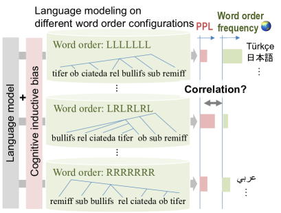
Figure 1: We compare the word orders challenging for LMs to those infrequent in attested languages (§ 3). We examine the advantage of cognitively motivated LMs (§ 4) in simulating the word-order universals (the world’s word-order distribution) with their inductive biases (§ 5).

In this study, expanding on a study of word-order biases in language models (LMs) White and Cotterell (2021), we demonstrate the advantage of cognitively-motivated LMs, which can simulate human cognitive load during sentence processing well Hale et al. (2018); Futrell et al. (2020a); Yoshida et al. (2021); Kuribayashi et al. (2022), and thus predict many implicational word-order universals in terms of their inductive biases. Specifically, we train various types of LMs in artificial languages with different word-order configurations (§ 3). Our experiments show that perplexities estimated by LMs with cognitively motivated biases (i.e., syntactic biases, specific parsing strategies, and memory limitations) (§ 4) correlate better with frequent word-order configurations in attested languages than standard LMs (§ 5). Our experimental results confirm that such biases are a potential source of the word-order universals, as well as demonstrate the advantage of cognitively motivated LMs as models of human language processing.

2 Related research

2.1 Impossible languages and LMs

Generative linguistic theory has traditionally focussed on delineating the impossible from possible languages in terms of universal grammar. Chomsky et al. (2023) has recently argued that neural LMs cannot distinguish possible human languages from impossible, unnatural languages, based on the experiments by Mitchell and Bowers (2020), and are, therefore, of no interest to linguistic theory. Kallini et al. (2024) challenge this claim, demonstrating that a standard transformer-based autoregressive model (GPT-2) assigns higher perplexity and greater surprisal to a range of artificially-generated, unattested and thus putatively impossible candidate languages when compared to English. In this work, by contrast, we explore the ability of a variety of neural LMs to distinguish typologically rare combinations of word orders from the common attested combinations as predicted by Greenberg’s implicational universals Greenberg et al. (1963).

2.2 The Chomsky hierarchy and LMs

We test how easy it is to learn a specific artificial language (with a specific word-order configuration) for certain LMs. Such exploration is related to the investigation of the capabilities of neural LMs to generate formal, artificial languages in a specific class of the Chomsky hierarchy, such as irreducibly context-free (such as the Dyck languages) or mildly context-sensitive (such as aⁿbⁿcⁿ) languages Weiss et al. (2018); Suzgun et al. (2019); Hewitt et al. (2020); Deletang et al. (2022). While this line of research can elucidate whether specific models (LSTMs, Transformers, etc.) are capable in principle of expressing and generalizing such languages, and thus also generating their putative analogs in natural language, in this work we focus on artificial languages which are more human language-like in that they exhibit a range of attested construction types, a more realistic vocabulary, and are less marked in terms of features like average sentence length, at least compared to the formal languages adopted in this line of research (App. A).

2.3 Word order preferences of LMs

Researchers have asked what kind of language is hard to language-model Cotterell et al. (2018); Mielke et al. (2019), motivated by concern over whether the current language-modeling paradigm is equally suitable for all languages. However, experiments using only attested language corpora made it difficult to single out impactful factors since attested languages differ from each other in multiple dimensions Cotterell et al. (2018); Mielke et al. (2019). Thus, prior studies adopted the use of artificially controlled language(-like) data as a lens to quantify the inductive bias of models Wang and Eisner (2016); White and Cotterell (2021); Hopkins (2022). Specifically, White and Cotterell (2021) pointed out some differences between LM’s word-order preferences and common attested word orders (typological markedness). We expand on their research by exploring which models, including cognitively motivated ones, exhibit preferences more aligned with common typological patterns.

2.4 Cognitively motivated LMs

Computational psycholinguists have explored LMs mirroring the cognitive load of human sentence processing Goodkind and Bicknell (2018); Wilcox et al. (2020); Oh and Schuler (2023). For example, the syntactic biases, parsing strategies, and memory limitations exhibited are of interest Hale et al. (2018); Yoshida et al. (2021); Futrell et al. (2020a); Kuribayashi et al. (2022); Oh et al. (2024). We demonstrate their advantage in the computational simulation of typological markedness of word orders. Such psycholinguistic findings are typically overlooked in the line of emergent language research Lian et al. (2023).

3 Experimental design

We explain the assumptions behind this research in § 3.1. Then, we confirm the word-order biases in human languages in § 3.2 and investigate how well a particular LM simulates the attested word-order biases in § 3.3.

3.1 Preliminary

Given the theory that language has evolved to promote its processing efficiency Hawkins (2004); Gibson et al. (2019), we posit that the frequency ($\mathrm{Freq}$) of a word order $o$ will be proportional to the negative of effort required to process it:

$$\mathrm{Freq}(o) \propto-\mathrm{Effort}(o)\;\;\mathrm{.}$$ (1)

We further posit that processing effort is determined by the predictability of a word in context $p(w_{k}|\boldsymbol{w}_{<k})$, based on expectation-based theory Levy (2008); Smith and Levy (2013). Thus, we estimate the processing difficulty of a word-order configuration $o$ by measuring the average processing effort required to process sentences with word order $o$. This can be quantified by perplexity (PPL), the geometric mean of word predictability, of a corpus $L_{o}$ following the word order $o$:

$$\mathrm{Effort}(o) \sim\underset{w_{i}\in L_{o}}{\prod}p_{\theta}(w_{i}|\boldsymbol{w}_{<i})^{-\frac{1}{|L_{o}|}}\;\;\mathrm{.}$$ (2)

Here, the probability is computed by an LM $\theta$. We analyze what word order incurs more processing costs for particular LMs.

Note that, more generally, human language is arguably designed to minimize complexity (how unpredictable symbols are) while maintaining informativity (how easy it is to extract a message from symbols) (i Cancho and Solé (2003); Piantadosi et al. (2012); Kemp and Regier (2012); Frank and Goodman (2012); Kirby et al. (2015); Kanwal et al. (2017); Gibson et al. (2019); Xu et al. (2020); Hahn et al. (2020); inter alia). The connection to this bi-dimensional view is analyzed in § 7.1.

3.2 Word order biases in attested languages

Branching directionality:

Branching directionality, the concept of whether a dependent phrase is positioned left (L) or right (R) of its head in a particular constituent, is a key component of typological theory. For example, suppose a noun phrase ($\boldsymbol{\mathrm{NP}}$) and a verb phrase ($\boldsymbol{\mathrm{VP}}$) are dependent and head phrases, respectively. The word order of $\boldsymbol{\mathrm{NP}}\ \boldsymbol{\mathrm{VP}}$ is left-branching, while $\boldsymbol{\mathrm{VP}}\ \boldsymbol{\mathrm{NP}}$ is right-branching. Based on such branching directionalities, attested languages can be classified based on six different parameters (Table 1); for example, the parameter $s^{\boldsymbol{\mathrm{S}}}$ determines the order of the subject $\boldsymbol{\mathrm{NP}}$ and the $\boldsymbol{\mathrm{VP}}$. The six parameters result in $2^{6}=64$ types of word-order configurations $\mathcal{O}$; each order $o\in\mathcal{O}$ is denoted by a sequence of L/R in the order of $[s^{\boldsymbol{\mathrm{S}}}_{i},s^{\boldsymbol{\mathrm{VP}}}_{i},s^{\boldsymbol{\mathrm{PP}}}_{i},s^{\boldsymbol{\mathrm{NP}}}_{i},s^{\boldsymbol{\mathrm{Rel}}}_{i},s^{\boldsymbol{\mathrm{Case}}}_{i}]$. For example, LRLLLR $\in\mathcal{O}$ is the configuration where all phrases, except for $\boldsymbol{\mathrm{VP}}$ and $\boldsymbol{\mathrm{Case}}$, are left-branching.

Param.	L	R
$s^{\boldsymbol{\mathrm{S}}}$	Cat eats.	Eats cat.
$s^{\boldsymbol{\mathrm{VP}}}$	Cat mouse eats.	Cat eats mouse.
$s^{\boldsymbol{\mathrm{PP}}}$	Cat table on eats.	Cat on table eats.
$s^{\boldsymbol{\mathrm{NP}}}$	Small cat eats.	Cat small eats.
$s^{\boldsymbol{\mathrm{Rel}}}$	Likes milk that cat eats.	Cat that likes milk eats.
$s^{\boldsymbol{\mathrm{Case}}}$	Cat-sub eats.	Sub-cat eats.

Table 1: Word-order parameters and example constructions with different assignments, L or R (See Apps. A and B and White and Cotterell (2021) for details).

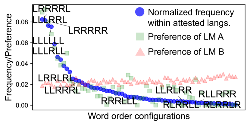
Figure 2: The frequency distribution of $64=2^{6}$ word-order configurations within attested languages (blue points) sorted in descending order. Suppose particular LMs A/B prefer word order as green/red points. The LM A (green points) is considered to have typologically more aligned inductive bias than the LM B (red points).

Word-order universals:

The 64 word-order configurations are not uniformly distributed among attested languages (blue points in Figure 2). This distribution is estimated by the frequency of word orders in The World Atlas of Language Structures (WALS) Dryer and Haspelmath (2013), which is also denoted as a vector $\boldsymbol{f}=[\mathrm{freq}(\texttt{LLLLLL}),\mathrm{freq}(\texttt{LLLLLR}),\cdots,\mathrm{freq}(\texttt{RRRRRR})]$. Notably, particular configurations, typically with harmonic (consistent) branching-directionality (e.g., LLLLLL, LRRRRR), are common; such a skewed distribution (typological markedness or word-order universals) has been studied from multiple perspectives typically tied with human cognitive biases Vennemann (1974); Gibson et al. (2000); Briscoe (2000); Levy (2005); Christiansen and Chater (2008); Culbertson et al. (2012); Temperley and Gildea (2018); Futrell and Levy (2019); Futrell et al. (2020b). We aim to simulate the word-order universals with LMs’ inductive biases.

3.3 Word order biases in LMs

Artificial languages:

We quantify which word orders are harder for a particular LM. Here, we adopt the set of artificial languages $\mathcal{L}$ created by White and Cotterell (2021) as a lens to quantify the LMs’ biases. These languages share the same default probabilistic context-free grammar and differ from each other only in their word-order configuration $o\in\mathcal{O}$ (§ 3.2) overriding the word order rules in the default grammar, resulting in 64 corpora with different word order $o$. Note that the 64 corpora generated have the same probabilities under the respective grammar; thus, differences in language-modeling difficulties can only stem from the model’s biases. See App. A for the detailed configurations of artificial languages.

Word-order preferences of LMs:

We train an LM on each corpus (word order $o$) and measure the PPL of tokens $\boldsymbol{x}$ in the respective held-out set. Repeatedly conducting the training/evaluation across the 64 corpora produces a PPL score vector, $\boldsymbol{p}=[\mathrm{PPL}_{\texttt{LLLLLL}}(\boldsymbol{x}),\mathrm{PPL}_{\texttt{LLLLLR}}(\boldsymbol{x}),\cdots,\mathrm{PPL}_{\texttt{RRRRRR}}(\boldsymbol{x})]$, which indicates that the word-order preferences of an LM.

3.4 Metrics

Global correlation:

We measure the Pearson correlation coefficient between negative PPL $-\boldsymbol{p}$ (§ 3.3) and their respective word order frequencies $\boldsymbol{f}$ (§ 3.2), $\mathrm{Corr}(-\boldsymbol{p},\boldsymbol{f})$ (henceforth, global correlation), considering lower PPL is better. A high global correlation indicates that the LMs’ word-order preferences reflect typological markedness.

Local correlation:

White and Cotterell (2021) reported that simulating the word-order distribution among subject, object, and verb (SOV$\succ$SVO$\succ$VOS$\succ$OVS), which is determined by the first two parameters of $s^{\boldsymbol{\mathrm{S}}}$ and $s^{\boldsymbol{\mathrm{VP}}}$, is challenging. First, therefore, we assess how easy it is to simulate the markedness of the other parameters’ assignments. Specifically, we measure a relaxed version of the correlation ignoring the subject, object, and verb order (local correlation), which is defined by the averaged correlation within each base word-order group: SOV (LL...), SVO (LR...), OVS (RL...), and VOS (RR...).

$$\begin{split}&\frac{1}{4}(\mathrm{Corr}(-\boldsymbol{p}_{\texttt{LL}},\boldsymbol{f}_{\texttt{LL}})+\mathrm{Corr}(-\boldsymbol{p}_{\texttt{LR}},\boldsymbol{f}_{\texttt{LR}})\\ &+\mathrm{Corr}(-\boldsymbol{p}_{\texttt{RL}},\boldsymbol{f}_{\texttt{RL}})+\mathrm{Corr}(-\boldsymbol{p}_{\texttt{RR}},\boldsymbol{f}_{\texttt{RR}}))\;\;\mathrm{.}\end{split}$$ (3)

Here, $\boldsymbol{p}_{\texttt{XY}}$ and $\boldsymbol{f}_{\texttt{XY}}$ are the list of perplexities and frequencies, limited to the languages with $s^{\boldsymbol{\mathrm{S}}}=\texttt{X}$ and $s^{\boldsymbol{\mathrm{VP}}}=\texttt{Y}$. If this relaxed correlation is high and the global correlation is low, the ordering of subject, object, and verb remains challenging.

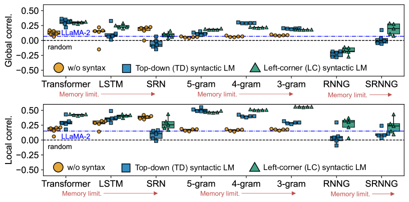
Figure 3: The results of global/local correlations. Each point corresponds to each run. Their colors and shapes denote the syntactic bias of the models. The TD and LC variants in the Transformer, LSTM, SRN, and N-gram settings correspond to the respective PLMs. The box presents the lower/upper quartiles.

4 Models

We examine 23 types of LMs. All the models are uni-directional and trained with subwords split by byte-pair-encoding Sennrich et al. (2016). See App. C for model details.

4.1 Standard LMs

We test the PPL estimated by a Transformer Vaswani et al. (2017), LSTM Hochreiter and Schmidhuber (1997), simple recurrent neural network (SRN) Elman (1990), and N-gram LMs. See § C.2 for the model details.

4.2 Cognitively motivated LMs

We further test cognitively motivated LMs employed in cognitive modeling and incremental parsing. We target three properties: (i) syntactic inductive/processing bias, (ii) parsing strategy, and (iii) working memory limitations, following recent works in cognitive modeling research Dyer et al. (2016); Hale et al. (2018); Resnik (1992); Oh et al. (2021); Yoshida et al. (2021); Futrell et al. (2020a); Kuribayashi et al. (2022).

Syntactic LMs and parsing strategy:

We begin with syntactic LMs to explore the cognitively-motivated LMs. They jointly model tokens $\boldsymbol{x}$ and their syntactic structures $\boldsymbol{y}$ by incrementally predicting parsing actions $\boldsymbol{a}$, such as “NT($\mathrm{S}$) NT($\mathrm{NP}$) GEN(I) REDUCE($\mathrm{NP}$)...’’:

$$p(\boldsymbol{x},\boldsymbol{y}) =\prod_{t}p(a_{t}|\boldsymbol{a}_{<t})\;\;\;\mathrm{.}$$ (4)

Here, we examine two commonly-adopted strategies to convert the $(\boldsymbol{x},\boldsymbol{y})$ into the actions $\boldsymbol{a}$: top-down (TD) and left-corner (LC) strategies. The LC strategy is theoretically expected to estimate more human-like cognitive loads than the TD Abney and Johnson (1991); Resnik (1992).

Memory limitation:

In addition to syntactic biases, we focus on memory limitations as human-like biases. Humans generally have limited working memory Miller (1956) and struggle with processing long-distance dependencies during sentence processing Hawkins (1994); Gibson et al. (2019); Hahn et al. (2021). We thus expect that model architectures with more severe memory access, e.g., in the order of SRN$\succ$LSTM$\succ$Transformer, have such human-like biases and exhibit higher correlations with the word-order universals.

Implementations:

We use the Parsing-as-Language-Model (PLM) Choe and Charniak (2016) and recurrent neural network grammar (RNNG) Dyer et al. (2016); Kuncoro et al. (2017). PLMs have the same architectures as standard LMs but are trained on the action sequences $\boldsymbol{a}$. We examine four PLMs with different architectures (Transformer, LSTM, SRN, and N-gram). RNNGs also predict the action sequences, but they have an explicit composition function to compute phrase representations. We use the stack-only RNNG implementation by Noji and Oseki (2021) and its memory-limited version (simple recurrent neural network grammar; SRNNG), where (Bi)LSTMs are replaced by SRNs. Henceforth, syntactic LMs refer to the PLMs and (S)RNNGs.

PPL:

We measure the PPL over action sequences in each word order $o$ when quantifying the word-order preference of syntactic LMs (§ 3.3): $\mathrm{PPL}_{o}(\boldsymbol{x},\boldsymbol{y}):=\prod_{t}p(a_{t}|\boldsymbol{a}_{<t})^{\frac{1}{|\boldsymbol{a}|}}$. We also examine a token-level predictability $\mathrm{PPL}_{o}(\boldsymbol{x})$ in § 7.1 and § D.1, but such variations did not alter the conclusions.

4.3 Baselines

We set two baselines: (i) a chance rate with random assignments of perplexities (gray lines), and (ii) perplexities estimated by pre-trained LLaMA-2 (7B) Touvron et al. (2023), a representative of the large language models (LLMs), prompted with several example sentences (blue lines) (§ C.3) as a naive baseline.

5 Experiment

We compare the LM’s word-order preferences with attested word-order distributions (§ 5). Then, we further analyze what kind of word-order combinations LMs prefer (§ 6) and discuss connections between our observations and existing studies (§ 7).

5.1 Settings

For each LM, we report the mean and standard deviation across five runs with different random seeds. In each run, 20K sentences are generated and split into train/dev/test sets with an 8:1:1 ratio.

5.2 Results

Figure 3 shows global and local correlations (see App. D for the full results). The TD (blue) and LC (green) variations of the Transformer, LSTM, SRN, and N-gram LMs correspond to the PLMs with their respective architecture. We expect syntactic LMs with the LC strategy (green) to exhibit higher correlations than the LMs without syntactic biases (orange) or those with cognitively unmotivated TD syntactic bias (blue).

Most LMs beat the chance rate:

Overall, most global and local correlations were higher than the random baseline, reproducing the general trend that common word orders induce lower PPL Hahn et al. (2020). As a sanity check, we also observed that the LLaMA-2 exhibited weaker correlations than cognitively motivated LMs; the current success of LLMs is orthogonal to our results.

Syntactic biases and parsing strategies:

First, the LC syntactic LMs (green points) generally outperformed the standard LMs (orange points) in each setting except for SRNs. This indicates the advantage of cognitively-motivated syntactic biases in simulating the word-order universals. Second, LMs with the LC strategy (green points) tend to exhibit higher correlations than TD syntactic LMs (blue points), especially in terms of local correlation. That is, the cognitively motivated LC parsing strategy better simulates the word-order implicational universals. Note that RNNGs, on average, exhibited low correlations, although they are often claimed to be cognitively plausible LMs.

Memory limitation:

The results show that memory-limited models tend to exhibit better correlations, with the exception of PLMs. In particular, while RNNGs typically benefited from memory limitations (SRNNG$\succ$RNNG), PLMs did not (SRN$\prec$Transformer). This implies a superiority of RNNGs’ memory decay over hierarchical tree encoding to PLMs’ simple linear memory decay.

5.3 Regression analysis

We test the statistical significance of the contribution of cognitively-motivated factors to higher correlations. Specifically, we train the following regression model to predict the global or local correlation scores obtained in the experiment (§ 5.2):

$$\begin{split}\mathrm{Correl}_{\theta}\sim&\ \mathrm{ModelClass}(\theta)+\mathrm{MemLim}(\theta)\\ &+\mathrm{Syntax}(\theta)+\mathrm{LC}(\theta)\;\;\mathrm{.}\end{split}$$ (5)

Here, $\mathrm{ModelClass}$ denotes the coarse type (e.g., neural model or not) of the model $\theta$ yielding the respective correlation score, $\mathrm{MemLim}$ denotes its strength of context limitation (higher is severer, e.g., SRN$\succ$LSTM$\succ$Transformer), $\mathrm{Syntax}$ denotes whether the model is syntactic LMs (1 for syntactic LMs; otherwise 0), and $\mathrm{LC}$ denotes whether the model uses the LC strategy (1 for LC syntactic LMs; otherwise 0). Positive coefficients for these features indicate their contribution to higher correlations. See App. E for the details of the regression.

We observe that the coefficients for the $\mathrm{Syntax}$ and $\mathrm{LC}$ features were significantly larger than zero with one-sample, two-sided t-test in both cases of predicting global and local correlations. The coefficient for the $\mathrm{MemLim}$ feature was not significantly larger than zero when targeting all the models ($p>0.1$); however, when PLMs were excluded, the coefficient of the $\mathrm{MemLim}$ feature was also significantly larger than zero with one-sample, two-sided t-test ($p<0.001$ in both global and local correlations) as suggested in § 5.2. To sum up, these corroborate the findings in § 5.2.

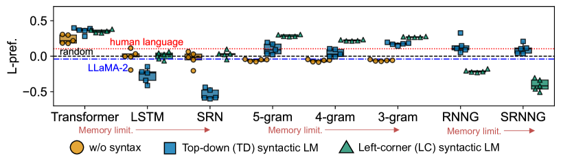
Figure 4: The results of branching directionality scores. Each point corresponds to each run. The colors and shapes denote the syntactic bias of the models. The TD and LC variants in the Transformer, LSTM, SRN, and N-gram settings correspond to the respective PLMs. The box presents the lower/upper quartiles.

6 Analyses

6.1 Branching directionality preferences

Human languages, on average, do not favor either left- or right-branching Dryer and Haspelmath (2013). Given this, we measure how strongly a model prefers a specific branching directionality (L-pref.). We calculate the Pearson correlation between negative PPL and the number of L assignments $\mathrm{\#}\texttt{L}(\cdot)$ of the respective word order:

$$\mathrm{Corr}(-\boldsymbol{p},\boldsymbol{b})\;\;\mathrm{,}$$ (6)

$$\boldsymbol{b}:=[\mathrm{\#}\texttt{L}(l)\ \mathrm{for}\ l\ \mathrm{in}\ \mathcal{L}]\;\;\mathrm{.}$$ (7)

As a sanity check, the word-order frequency distribution of attested languages, indeed, is weakly correlated (0.11) with the left-branching directionality. Thus, LMs are not expected to have an extremely high or low L-pref. score. Notably, the branching bias of LMs/parsers has been of interest in the NLP research Li et al. (2020a, b); Ishii and Miyao (2023).

Results:

Figure 4 shows the results of branching preferences. LMs with the TD strategy are theoretically expected to have a lower L-pref. score (favoring right-branching) than the LC models Resnik (1992). While the PLMs faithfully reflect such characteristics, RNNGs, surprisingly, exhibited opposite trends, suggesting the challenge in controlling the inductive bias of neural syntactic LMs. We also observed architecture-dependent branching preference; Transformers prefer left-branching, while LSTMs prefer right-branching as suggested by Hopkins (2022). Such architecture-dependent biases seem to have more impact on the branching preferences than the parsing strategies in PLMs.

6.2 Linking functions

The experiments so far have assumed the linearity between PPL and word-order frequency (Eq. 1)—did this choice bias our results? We investigated various linking functions between PPL and word order frequency: the perplexity of order $k$ and logarithmic PPL (entropy). Figure 5 illustrates LMs’ local correlations under differently converted perplexities; full results are in Appendix D.2. Such a variation of linking functions did not substantially affect our results (§ 5), enhancing the generality of our obtained findings.

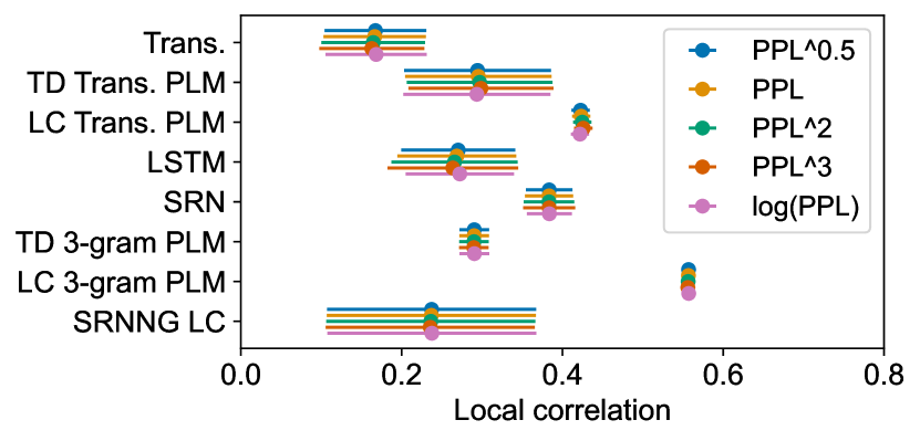
Figure 5: Mean and standard deviation of local correlations with different linking functions: PPL of order $k$ and logarithmic PPL

7 Discussion

7.1 Predictability and parsability

We revisit the view that both predictability and parsability are keys to explaining word-order universals. Concretely, Hahn et al. (2020) showed that both PPL of an LM and parsability for a (not-cognitively-motivated) parser Kiperwasser and Goldberg (2016) explain word-order universals. Building on this, we demonstrate that predictability (PPL) of syntactic LMs entails parsability. That is, they can provide a more concise information-theoretic measurement of word-order universals (syntactically-biased predictability).

Specifically, we decompose the performance of syntactic LMs into two parts: token-level perplexity $\mathrm{PPL}(\boldsymbol{x})$ (predictability) and parsing performance $\mathrm{Parse}(\boldsymbol{x},\boldsymbol{y})$ (parsability), using word-synchronous beam-search Stern et al. (2017). When computing the token-level predictability $\mathrm{PPL}(\boldsymbol{x})$, next-word probability is computed while predicting the upcoming partial syntactic trees. We measure $\mathrm{Parse}(\boldsymbol{x},\boldsymbol{y})$ as the F1-score of the top-1 parse found with the beam search. Then, we test whether the parsability factor contributes to explaining the frequency of word order $o$ in addition to PPL, using the following nested regression models:

$$\mathrm{\textbf{Base:}}\ \mathrm{Freq}(o) \sim\mathrm{PPL}_{o}(\boldsymbol{x})\;\;\mathrm{,}$$

$$\mathrm{\textbf{+Parse:}}\ \mathrm{Freq}(o) \sim\mathrm{PPL}_{o}(\boldsymbol{x})+\mathrm{Parse}_{o}(\boldsymbol{x},\boldsymbol{y})\;\;\mathrm{.}$$

The increase in log-likelihood scores of the +Parse model over the Base model is not significant with the likelihood-ratio test ($p>0.1$) in all the RNNG settings ({TD, LC}$\times${SRNNG, RNNG}$\times${seeds}). That is, at least in our setting, we cannot find an advantag of parsability over predictability in explaining word-order universals. This may be because the next-word prediction for the syntactic LMs is explicitly conditioned by the parsing states, which might sufficiently bias the predictability measurements to reflect parsability.

Figure 6 also illustrates the predictability and parsability estimated by the LC SRNNG. Here, the predictability identifies more types of word orders as typologically marked (left small circles) than the parsability does (bottom small circles). This is contrary to the picture of both predictability and parsability as complementary factors explaining word-order universals Hahn et al. (2020).

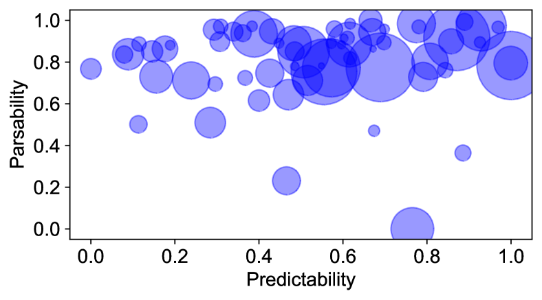
Figure 6: Predictability and parsability of each word order. These measurements are converted through the min-max normalization to be [0, 1] scale (higher is better). Each circle corresponds to each word order; larger ones are frequent word orders.

7.2 {S,O,V} word-order biases

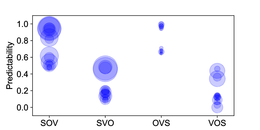
Figure 7: Illustration of the relationship between predictability (y-axis) and word order frequency in each of the four base-order groups (SOV, SVO, OVS, and VOS). Each circle corresponds to each word order; larger ones are frequent word orders. Predictability is the negative PPLs converted through the min-max normalization; thus higher predictability indicates lower PPL. The results are from the 3-gram PLM with the LC strategy.

White and Cotterell (2021) reported that LMs could not show the subject, object, verb word-order biases attested in natural language (SOV$\succ$SVO$\succ$VOS$\succ$OVS). Even our cognitively-motivated LMs did not overcome this limitation, based on the global correlations being consistently lower than the local ones (§ 5.2; Figure 3). This tendency is visualized in Figure 7; within each base group (SOV, SVO, OVS, VOS), common word orders tend to obtain high predictability (i.e., lower PPL; bigger circles are at the top) except OVS-order’s high predictability and SVO-order’s low predictability. This made it clear that predictability generally explains word-order universals, but the markedness of word orders among subject, object, and verb must stem from additional factors.

Humans arguably have an actor-first bias in event cognition, and this could be the source of the subject-initial word order Wilson et al. (2022). Our findings imply that cognitively motivated LMs still lack such a human-like bias. Orthogonally, the artificial language ignores some important linguistic aspects, such as information structure Gundel (1988); Verhoeven (2015); Ranjan et al. (2022), which may explain subject-object order; refining the artificial data would also be one direction to explore in future work.

8 Conclusions

We have investigated the advantages of cognitively-motivated LMs in the computational simulation of emergent word-order universals. From a linguistic typology perspective, we provide computational evidence of the universals emerging from cognitive biases, which has been challenging to demonstrate in previous work Lian et al. (2021); Galke et al. (2022). From the cognitive modeling perspective, our results demonstrate that cognitively motivated LMs have human-like biases that are sufficient to replicate some human word-order universals. From the natural language processing perspective, we clarify the inductive bias of various classes of LMs.

Limitations

Artificial data:

We used artificial data to quantify the LMs’ inductive/processing biases for word-order configurations. While the use of artificial languages has typically been adopted to conduct controlled experiments (§ 2.2), such artificial data lack some properties of natural languages, such as the semantic relationships between the linguistic constituents and discourse-level factors (§ 7.2). In future work, we hope to devise further artificially controlled languages that exhibit some of these properties. Furthermore, our used data White and Cotterell (2021) is relatively small scale, which might incur unintended bias in LM performance, although there is a perspective to analyze inductive bias via measuring training efficiency Kharitonov and Chaabouni (2021); Warstadt et al. (2023).

Estimating word-order distribution:

The word order frequency estimates derived from WALS might also be biased; for example, Indo-European languages tend to have richer meta-linguistic information in WALS, although our study takes the statistics from as many as 1,616 languages into account. A richer estimation of missing parameter information is desirable. As a more general concern, the frequency of a word-order configuration can be estimated in various ways, such as the number of native speakers and the number of language families adopting a particular word order. Furthermore, word order variation can be inherently non-binary Levshina et al. (2023). Our study, as an initial foray, relied on the number of unique languages, a commonly used metric in linguistic typology research Dryer and Haspelmath (2013); Hammarström (2016), considering that other approaches raise additional complications, such as an estimation of the speaker numbers or language family variability.

Ethics Statement

We only used artificial language, which does not have information with potential risks, e.g., human privacy data. One concern is the bias in our word order frequency estimates; this might have brought biased conclusions, e.g., diminishing the impact of minority languages, although we used the largest publicly available data (WALS) to date. We used AI assistance tools within the scope of “Assistance purely with the language of the paper” described in the ACL 2023 Policy on AI Writing Assistance.

	Right-branching	Mixed-branching	Left-branching
Parameteres	RRRRRR	LRRRLR	LLLLLL
	[.$\mathrm{S}$ [.$\mathrm{VP}$ [.$\mathrm{Verb}$ strovokicizeda ] !1cm ] !2cm [.$\mathrm{NP}$ [.$\mathrm{NP}$ fusbenders ] !1cm [.$\mathrm{Rel}$ rel ] !0.5cm [.$\mathrm{VP}$ [.$\mathrm{Verb}$ povify ] !1cm [.$\mathrm{NP}$ [.$\mathrm{Pronoun}$ me ] ] !1cm ] !1.5cm ] !2cm ]	[.$\mathrm{S}$ [.$\mathrm{NP}$ [.$\mathrm{NP}$ fusbenders ] !0.5cm [.$\mathrm{Rel}$ rel ] !1cm [.$\mathrm{VP}$ [.$\mathrm{Verb}$ povify ] [.$\mathrm{NP}$ [.$\mathrm{Pronoun}$ me ] !0.5cm ] ] !1.1cm ] [.$\mathrm{VP}$ [.$\mathrm{Verb}$ strovokicizeda ] ] !0.5cm ]	[.$\mathrm{S}$ [.$\mathrm{NP}$ [.$\mathrm{VP}$ [.$\mathrm{NP}$ [.$\mathrm{Pronoun}$ me ] ] !1cm [.$\mathrm{Verb}$ povify ] ] [.$\mathrm{Rel}$ rel ] !0.5cm [.$\mathrm{NP}$ fusbenders ] !1cm ] !1.5cm [.$\mathrm{VP}$ [.$\mathrm{Verb}$ strovokicizeda ] ] !2cm ]

Table 2: Example sentences and their structures generated with different word-order configurations.

Appendix A Details of artificial languages

Table 12 shows the default grammar to create artificial language data, which adopts the configuration of White and Cotterell (2021). The “relevant parameter” column indicates that the listed parameter controls the order of right-hand items in the respective production rule (the order is swapped when the parameter assignment is R). Note that the subcategory of non-terminal symbols (e.g., $\mathrm{VP}\_\mathrm{S}$) was only used for generating the data; in the final data for training/evaluating syntactic LMs, these subcategories are omitted (e.g., $\mathrm{VP}\_\mathrm{S}$ should be $\mathrm{VP}$), and the resulting uninformative edge in the syntactic structure (e.g., $\mathrm{VP}\rightarrow\mathrm{VP}$) was removed. Table 2 shows the example of a sentence with different word-order configurations. Different word order parameters yield a syntactic structure with different branching directionalities; for example, the constituency tree of LLLLLL is extending to the bottom left (left-branching). The average sentence length was 11.8 tokens, and the average tree depth was 9.1. The vocabulary size of pseudowords is 1,314 same as White and Cotterell (2021).

All languages in WALS	2,679
Targeted languages	1,616
Targeted parameters	9,696 (=1,616$\times$6)
Missing parameters	3,343
LLXXXX (SOV)	46.7%
LRXXXX (SVO)	34.3%
RLXXXX (VOS)	3.6%
RRXXXX (OVS)	15.5%
$s^{\boldsymbol{\mathrm{S}}}$ ($\boldsymbol{\mathrm{S}}\rightarrow\boldsymbol{\mathrm{NP}}_{\textbf{subj}}\ \boldsymbol{\mathrm{VP}}$)	82A Order of Subject and Verb Dryer (2013e)
$s^{\boldsymbol{\mathrm{VP}}}$ ($\boldsymbol{\mathrm{VP}}\rightarrow\boldsymbol{\mathrm{NP}}_{\textbf{obj}}\ \textbf{Verb}$)	83A Order of Object and Verb Dryer (2013c)
$s^{\boldsymbol{\mathrm{PP}}}$ ($\boldsymbol{\mathrm{PP}}\rightarrow\textbf{Prep}\ \boldsymbol{\mathrm{NP}}$)	85A Order of Adposition and Noun Phrase Dryer (2013b)
$s^{\boldsymbol{\mathrm{NP}}}$ ($\boldsymbol{\mathrm{NP}}\rightarrow\textbf{Adj}\ \boldsymbol{\mathrm{NP}}$)	87A Order of Adjective and Noun Dryer (2013a)
$s^{\boldsymbol{\mathrm{Rel}}}$ ($\boldsymbol{\mathrm{NP}}\rightarrow\boldsymbol{\mathrm{VP}}\ \textbf{Rel}\ \boldsymbol{\mathrm{NP}}$)	90A Order of Relative Clause and Noun Dryer (2013d)
$s^{\boldsymbol{\mathrm{Case}}}$ ($\boldsymbol{\mathrm{NP}}\rightarrow\boldsymbol{\mathrm{NP}}\ \textbf{Case}$)	51A Position of Case Affixes Dryer (2013g)

Table 3: Statistics of the WALS data and the source of word-order configuration information

Appendix B WALS data statistics

Table 3 shows the statistics of the WALS data and the details about word order parameters. Out of the 2,679 languages listed in the WALS, 1,616 languages are involved, and approximately $2/3$ of their word order parameters were annotated in the WALS; the missing values are completed as explained in § 3.2 (footnote 1). As a sanity check, we observe the ratio of the assignments of the first two parameters ($\boldsymbol{s}^{\mathrm{S}}$ and $\boldsymbol{s}^{\mathrm{VP}}$), which controls the order of subject, object, and verb; these approximately replicate the ratio reported in Dryer (2013f) (e.g., SOV and SVO orders occupy over 80% of languages).

Data/model	Licence
Artificial data White and Cotterell (2021)	MIT
WALS Dryer and Haspelmath (2013)	Creative Commons CC-BY 4.0
Fairseq Ott et al. (2019)	MIT
RNNG Noji and Oseki (2021)	MIT
KenLM Heafield (2011)	LGPL
LLaMA-2 Touvron et al. (2023)	LLAMA 2 Community License
Sentencepiece Kudo and Richardson (2018)	Apache 2.0

Table 4: Licence of the data and models

Appendix C Model details

The license of the used models/data is listed in Table 4; all of them are used under their intended use. All the models were trained/tested with a single NVIDIA A100 GPU (40GB). All of the experiments were done within approximately 600 GPU hours. The LLaMA-2 (7B) model was used via the hugging face toolkit Wolf et al. (2020).

C.1 Parsing strategies

Figure 8 shows the parsing actions converted with different strategies (TD and LC). PLMs are trained to predict such a sequence of parsing actions in a left-to-right manner.

C.2 Hyperparamteres

Tables 13 and 14 show the hyperparameters of LMs,14 which basically follow their default settings. Standard LMs and PLMs use the same hyperparameters. Their vocabulary size is set to $512$.

C.3 Word order preference of LLaMA-2

We employed few-shot settings instead of full-finetning with the limits in computational cost. Specifically, we create a prompt consisting of the instruction “The below sentences are written in an artificially created new language:” and ten example sentences extracted from the respective training set. The probability of each test sentence is computed conditioned with this prompt, and aggregating these probabilities results in the PPL of an entire corpus.

Appendix D Results

The full results of the experiment (§ 5) and analysis (§ 6) are shown in Table 6. This also shows the top-3 preferred word orders by each LM, which demonstrates the model-dependent differences in their word-order preferences. We also include the baseline of average stack depth required to process sentences for each parsing algorithm in each word order as a standard measurement of memory cost.

D.1 Beam-search in RNNG/SRNNGs

Table 7 shows the results of RNNG/SRNNGs with and without word-synchronous beam search Stern et al. (2017). The settings without beam-search are adopted in § 5, and the advantages of memory limitation (SRRNG) and the LC strategies were replicated even with beam-search, where the token-level perplexity $\mathrm{PPL}(\boldsymbol{x})$ is used (§ 7.1).

D.2 Results with different linking functions

Tables 8, 9, 10, and 11 show the detailed results with different linking functions ($\mathrm{PPL}^{1/2}$, $\mathrm{PPL}^{2}$, $\mathrm{PPL}^{3}$, $\log\mathrm{PPL}$) between model-computed complexity measurements and word order frequencies. Experiments with different linking hypotheses did not alter the conclusions. This supports the generality of our findings.

Model	$\mathrm{ModelClass}$ (categorical)	$\mathrm{MemLim}$ (int)	$\mathrm{Syntax}$ (binary)	$\mathrm{LC}$       (binary)
Transformer	NLM	0	False	False
LSTM	NLM	1	False	False
SRN	NLM	2	False	False
Trans. PLM TD	NLM	0	True	False
Trans. PLM LC	NLM	0	True	True
LSTM PLM TD	NLM	1	True	False
LSTM PLM LC	NLM	1	True	True
SRN PLM TD	NLM	2	True	False
SRN PLM LC	NLM	2	True	True
Word 5-gram	CLM	0	False	False
Word 4-gram	CLM	1	False	False
Word 3-gram	CLM	2	False	False
5-gram PLM TD	CLM	0	True	False
5-gram PLM LC	CLM	0	True	True
4-gram PLM TD	CLM	1	True	False
4-gram PLM LC	CLM	1	True	True
3-gram PLM TD	CLM	2	True	False
3-gram PLM LC	CLM	2	True	True
RNNG	RNNG	0	True	False
RNNG LC	RNNG	0	True	True
SRNNG	RNNG	1	True	False
SRNNG LC	RNNG	1	True	True

Table 5: Features used for the regression analysis

Appendix E Details of regression analysis

We explored which factor impacts the global/local correlation scores obtained by various LMs $\theta$. As explained in § 5.3, we train a regression model to predict the correlation score obtained by a particular LM $\theta$, given the features characterizing the LMs:

$$\begin{split}\mathrm{Correl}_{\theta}\sim&\ \mathrm{ModelClass}(\theta)+\mathrm{MemLim}(\theta)\\ &+\mathrm{Syntax}(\theta)+\mathrm{LC}(\theta)\;\;\mathrm{.}\end{split}$$ (8)

Table 5 shows the features used for the regression analysis in § 5.3. The regression model is trained with the ordinary least squares setting, using statsmodel package in Python Seabold and Perktold (2010).

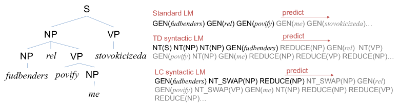
Figure 8: Different parsing strategy converts a syntactic structure into a different parsing action sequence. PLMs and RNNGs predict such action sequences with different model architectures.

Model	Lim.	Stx.	Global $r$  $\uparrow$	Local $r$  $\uparrow$	L-pref. $\rightarrow$	Top3 langs.
Natural Lang.			100.0	100.0	10.5	LRRRRL, LRRRRR, LLLRRL
Transformer			12.1 $\pm$ 4.3	16.7 $\pm$ 6.4	23.8 $\pm$ 6.1	LLLLLL, LLRLLL, RLRLLL
LSTM	✓		10.7 $\pm$ 14.7	26.9 $\pm$ 7.4	-1.2 $\pm$ 11.3	RLRLLL, RLLLLL, RRRRRR
SRN	✓		16.3 $\pm$ 9.4	38.3 $\pm$ 3.0	-3.6 $\pm$ 10.4	RLLLLL, RLRLLL, RLRRLL
Word 5-gram	✓		5.4 $\pm$ 1.0	17.0 $\pm$ 1.7	-5.8 $\pm$ 1.6	RRLRRR, RRRRRR, LRLRRR
Word 4-gram	✓		6.5 $\pm$ 1.0	16.5 $\pm$ 1.6	-6.4 $\pm$ 1.6	RRLRRR, RRRRRR, LRLRRR
Word 3-gram	✓		8.8 $\pm$ 0.7	17.5 $\pm$ 1.0	-6.1 $\pm$ 1.0	RRRRRR, RRLRRR, LRLRRR
Trans. PLM		TD	30.4 $\pm$ 5.7	29.5 $\pm$ 9.1	35.9 $\pm$ 4.7	LLRRLL, LLRRRL, LLRLLL
Trans. PLM		LC	30.3 $\pm$ 2.1	42.3 $\pm$ 1.1	35.2 $\pm$ 2.3	LLLLLL, LLRLLL, LLRRLL
LSTM PLM	✓	TD	11.9 $\pm$ 12.2	37.0 $\pm$ 7.3	-27.1 $\pm$ 10.5	LRRRRL, LRLRRL, LRRRRR
LSTM PLM	✓	LC	23.6 $\pm$ 3.6	40.4 $\pm$ 2.5	0.5 $\pm$ 5.5	RLLRRR, LLLLLL, LLLRLL
SRN PLM	✓	TD	-5.4 $\pm$ 8.3	8.7 $\pm$ 7.8	-53.7 $\pm$ 7.4	RLRRRR, LRLRRR, RLLRRR
SRN PLM	✓	LC	9.5 $\pm$ 4.9	27.5 $\pm$ 10.5	2.8 $\pm$ 5.2	RLRRLL, RLRRRR, RLLRLL
5-gram PLM	✓	TD	11.8 $\pm$ 2.4	50.4 $\pm$ 2.8	10.2 $\pm$ 7.8	RLLRRL, RLRRRL, RLLLLL
5-gram PLM	✓	LC	18.6 $\pm$ 0.9	47.0 $\pm$ 1.3	28.8 $\pm$ 1.4	LLLRLL, RLLRLL, RLRRLL
4-gram PLM	✓	TD	29.2 $\pm$ 0.6	40.0 $\pm$ 1.6	4.4 $\pm$ 5.4	LLRRRL, RLRRRL, LLRRRR
4-gram PLM	✓	LC	21.7 $\pm$ 0.6	50.6 $\pm$ 0.6	22.2 $\pm$ 0.9	RLLRLL, RLRRLL, LLLRLL
3-gram PLM	✓	TD	19.9 $\pm$ 0.7	29.0 $\pm$ 1.8	17.3 $\pm$ 2.0	RLLRRL, LLLRRL, RLLRRR
3-gram PLM	✓	LC	18.0 $\pm$ 0.2	55.7 $\pm$ 0.3	27.0 $\pm$ 0.5	RLLRRR, RLLRRL, RLRRRR
RNNG		TD	-22.6 $\pm$ 4.7	6.0 $\pm$ 14.5	14.5 $\pm$ 10.8	RLLRLL, RRRRLL, RRRLLL
RNNG		LC	-17.6 $\pm$ 6.4	25.1 $\pm$ 13.4	-21.2 $\pm$ 2.0	RRRRRL, RRLLRL, RRLRRL
SRNNG	✓	TD	2.0 $\pm$ 9.3	10.7 $\pm$ 7.8	10.2 $\pm$ 7.0	RLLRRR, RLRRRR, RLLRRL
SRNNG	✓	LC	19.0 $\pm$ 9.6	23.7 $\pm$ 13.0	-40.6 $\pm$ 8.5	LRRRRR, LRLRRR, LLLRRR
LLaMA2 (7B)			6.9 $\pm$ 31.0	15.4 $\pm$ 2.5	-4.6 $\pm$ 31.0	LRLLLL, LRRLLL, LRLRLL
Stack depth		TD	-47.5 $\pm$ 0.2	-12.0 $\pm$ 0.6	-56.2 $\pm$ 1.3	RRLRRR, RRLLRR, RRRRRR
Stack depth		LC	-13.3 $\pm$ 0.3	-4.8 $\pm$ 0.2	57.6 $\pm$ 0.5	RLLLLL, RLLRLL, RLRLLL
Chance rate			0.0	0.0	0.0	-

Table 6: Word-order preferences of LMs. “Lim.” and “Stx.” indicate the working memory limitation and syntactic biases in the respective model architecture, respectively.

Model	Syntax	Lim.	Beam	Global $r$  $\uparrow$	Local $r$  $\uparrow$	L-pref. $\rightarrow$	Top3 langs.
RNNG	TD			-22.6 $\pm$ 4.7	6.0 $\pm$ 14.5	14.5 $\pm$ 10.8	RLLRLL, RRRRLL, RRRLLL
SRNNG	TD	✓		2.0 $\pm$ 9.3	10.7 $\pm$ 7.8	10.2 $\pm$ 7.0	RLLRRR, RLRRRR, RLLRRL
RNNG	LC			-17.6 $\pm$ 6.4	25.1 $\pm$ 13.4	-21.2 $\pm$ 2.0	RRRRRL, RRLLRL, RRLRRL
SRNNG	LC	✓		19.0 $\pm$ 9.6	23.7 $\pm$ 13.0	-40.6 $\pm$ 8.5	LRRRRR, LRLRRR, LLLRRR
RNNG	TD		✓	9.4 $\pm$ 3.5	-31.5 $\pm$ 11.6	-30.1 $\pm$ 5.7	RRRRLL, RRRLLL, RRLLLL
SRNNG	TD	✓	✓	14.6 $\pm$ 8.7	-2.8 $\pm$ 5.9	-21.5 $\pm$ 8.9	LLLRRR, LLRRRR, RLRRRR
RNNG	LC		✓	-23.4 $\pm$ 7.0	26.5 $\pm$ 13.9	-26.2 $\pm$ 7.2	RLRLRL, RLRRLL, RRRRRL
SRNNG	LC	✓	✓	17.2 $\pm$ 8.5	18.3 $\pm$ 12.4	-36.7 $\pm$ 9.7	LRRRRR, LRLRRR, RLLRRR

Table 7: Comparson of the RNNG/SRNNG results with and without word-synchronous beam search

Model	Syntax	Lim.	Global $r$  $\uparrow$	Local $r$  $\uparrow$	L-pref. $\rightarrow$	Top3 langs.
Transformer			12.4 $\pm$ 4.3	16.7 $\pm$ 6.4	24.1 $\pm$ 6.1	LLLLLL, LLRLLL, RLRLLL
LSTM	✓		11.2 $\pm$ 14.7	27.0 $\pm$ 7.4	-0.8 $\pm$ 11.3	RLRLLL, RLLLLL, RRRRRR
SRN	✓		16.5 $\pm$ 9.4	38.4 $\pm$ 3.0	-3.5 $\pm$ 10.4	RLLLLL, RLRLLL, RLRRLL
Word 5-gram	✓		5.5 $\pm$ 1.0	17.1 $\pm$ 1.7	-6.0 $\pm$ 1.6	RRLRRR, RRRRRR, LRLRRR
Word 4-gram	✓		6.6 $\pm$ 1.0	16.7 $\pm$ 1.6	-6.7 $\pm$ 1.6	RRLRRR, RRRRRR, LRLRRR
Word 3-gram	✓		8.9 $\pm$ 0.7	17.7 $\pm$ 1.0	-6.3 $\pm$ 1.0	RRRRRR, RRLRRR, LRLRRR
Trans. PLM		TD	30.5 $\pm$ 5.7	29.4 $\pm$ 9.1	36.2 $\pm$ 4.7	LLRRLL, LLRRRL, LLRLLL
Trans. PLM		LC	30.2 $\pm$ 2.1	42.3 $\pm$ 1.1	35.7 $\pm$ 2.3	LLLLLL, LLRLLL, LLRRLL
LSTM PLM	✓	TD	11.9 $\pm$ 12.2	37.0 $\pm$ 7.3	-27.2 $\pm$ 10.5	LRRRRL, LRLRRL, LRRRRR
LSTM PLM	✓	LC	23.6 $\pm$ 3.6	40.4 $\pm$ 2.5	0.6 $\pm$ 5.5	RLLRRR, LLLLLL, LLLRLL
SRN PLM	✓	TD	-5.4 $\pm$ 8.3	8.8 $\pm$ 7.8	-53.8 $\pm$ 7.4	RLRRRR, LRLRRR, RLLRRR
SRN PLM	✓	LC	9.3 $\pm$ 4.9	27.6 $\pm$ 10.5	2.8 $\pm$ 5.2	RLRRLL, RLRRRR, RLLRLL
5-gram PLM	✓	TD	11.8 $\pm$ 2.4	50.5 $\pm$ 2.8	10.2 $\pm$ 7.8	RLLRRL, RLRRRL, RLLLLL
5-gram PLM	✓	LC	18.5 $\pm$ 0.9	47.0 $\pm$ 1.3	29.0 $\pm$ 1.4	LLLRLL, RLLRLL, RLRRLL
4-gram PLM	✓	TD	29.2 $\pm$ 0.6	40.0 $\pm$ 1.6	4.3 $\pm$ 5.4	LLRRRL, RLRRRL, LLRRRR
4-gram PLM	✓	LC	21.6 $\pm$ 0.6	50.5 $\pm$ 0.6	22.4 $\pm$ 0.9	RLLRLL, RLRRLL, LLLRLL
3-gram PLM	✓	TD	19.9 $\pm$ 0.7	29.0 $\pm$ 1.8	17.3 $\pm$ 2.0	RLLRRL, LLLRRL, RLLRRR
3-gram PLM	✓	LC	17.9 $\pm$ 0.2	55.7 $\pm$ 0.3	27.0 $\pm$ 0.5	RLLRRR, RLLRRL, RLRRRR
RNNG		TD	-22.6 $\pm$ 4.7	6.0 $\pm$ 14.5	14.5 $\pm$ 10.8	RLLRLL, RRRRLL, RRRLLL
RNNG		LC	-17.6 $\pm$ 6.4	25.1 $\pm$ 13.4	-21.1 $\pm$ 2.0	RRRRRL, RRLLRL, RRLRRL
SRNNG	✓	TD	1.9 $\pm$ 9.3	10.7 $\pm$ 7.8	10.1 $\pm$ 7.0	RLLRRR, RLRRRR, RLLRRL
SRNNG	✓	LC	19.1 $\pm$ 9.6	23.7 $\pm$ 13.0	-40.7 $\pm$ 8.5	LRRRRR, LRLRRR, LLLRRR
LLaMA2 (7B)			6.9 $\pm$ 31.0	15.4 $\pm$ 2.5	-4.6 $\pm$ 31.0	LRLLLL, LRRLLL, LRLRLL

Table 8: The results of $\mathrm{PPL}^{1/2}$

Model	Syntax	Lim.	Global $r$  $\uparrow$	Local $r$  $\uparrow$	L-pref. $\rightarrow$	Top3 langs.
Transformer			11.6 $\pm$ 4.3	16.5 $\pm$ 6.4	23.1 $\pm$ 6.1	LLLLLL, LLRLLL, RLRLLL
LSTM	✓		9.8 $\pm$ 14.7	26.6 $\pm$ 7.4	-1.8 $\pm$ 11.3	RLRLLL, RLLLLL, RRRRRR
SRN	✓		16.1 $\pm$ 9.4	38.3 $\pm$ 3.0	-3.6 $\pm$ 10.4	RLLLLL, RLRLLL, RLRRLL
Word 5-gram	✓		5.4 $\pm$ 1.0	16.7 $\pm$ 1.7	-5.3 $\pm$ 1.6	RRLRRR, RRRRRR, LRLRRR
Word 4-gram	✓		6.4 $\pm$ 1.0	16.1 $\pm$ 1.6	-5.8 $\pm$ 1.6	RRLRRR, RRRRRR, LRLRRR
Word 3-gram	✓		8.5 $\pm$ 0.7	17.1 $\pm$ 1.0	-5.6 $\pm$ 1.0	RRRRRR, RRLRRR, LRLRRR
Trans. PLM		TD	30.3 $\pm$ 5.7	29.7 $\pm$ 9.1	35.3 $\pm$ 4.7	LLRRLL, LLRRRL, LLRLLL
Trans. PLM		LC	30.3 $\pm$ 2.1	42.5 $\pm$ 1.1	34.1 $\pm$ 2.3	LLLLLL, LLRLLL, LLRRLL
LSTM PLM	✓	TD	11.8 $\pm$ 12.2	37.0 $\pm$ 7.3	-27.1 $\pm$ 10.5	LRRRRL, LRLRRL, LRRRRR
LSTM PLM	✓	LC	23.6 $\pm$ 3.6	40.4 $\pm$ 2.5	0.4 $\pm$ 5.5	RLLRRR, LLLLLL, LLLRLL
SRN PLM	✓	TD	-5.5 $\pm$ 8.3	8.7 $\pm$ 7.8	-53.7 $\pm$ 7.4	RLRRRR, LRLRRR, RLLRRR
SRN PLM	✓	LC	9.9 $\pm$ 4.9	27.4 $\pm$ 10.5	2.8 $\pm$ 5.2	RLRRLL, RLRRRR, RLLRLL
5-gram PLM	✓	TD	11.9 $\pm$ 2.4	50.4 $\pm$ 2.8	10.2 $\pm$ 7.8	RLLRRL, RLRRRL, RLLLLL
5-gram PLM	✓	LC	18.7 $\pm$ 0.9	47.1 $\pm$ 1.3	28.5 $\pm$ 1.4	LLLRLL, RLLRLL, RLRRLL
4-gram PLM	✓	TD	29.2 $\pm$ 0.6	40.0 $\pm$ 1.6	4.4 $\pm$ 5.4	LLRRRL, RLRRRL, LLRRRR
4-gram PLM	✓	LC	21.9 $\pm$ 0.6	50.6 $\pm$ 0.6	22.0 $\pm$ 0.9	RLLRLL, RLRRLL, LLLRLL
3-gram PLM	✓	TD	19.9 $\pm$ 0.7	29.0 $\pm$ 1.8	17.3 $\pm$ 2.0	RLLRRL, LLLRRL, RLLRRR
3-gram PLM	✓	LC	18.2 $\pm$ 0.2	55.6 $\pm$ 0.3	26.9 $\pm$ 0.5	RLLRRR, RLLRRL, RLRRRR
RNNG		TD	-22.6 $\pm$ 4.7	6.0 $\pm$ 14.5	14.5 $\pm$ 10.8	RLLRLL, RRRRLL, RRRLLL
RNNG		LC	-17.6 $\pm$ 6.4	25.1 $\pm$ 13.4	-21.2 $\pm$ 2.0	RRRRRL, RRLLRL, RRLRRL
SRNNG	✓	TD	2.1 $\pm$ 9.3	10.7 $\pm$ 7.8	10.2 $\pm$ 7.0	RLLRRR, RLRRRR, RLLRRL
SRNNG	✓	LC	19.0 $\pm$ 9.6	23.6 $\pm$ 13.0	-40.4 $\pm$ 8.5	LRRRRR, LRLRRR, LLLRRR
LLaMA2 (7B)			6.9 $\pm$ 31.0	15.5 $\pm$ 2.5	-4.8 $\pm$ 31.0	LRLLLL, LRRLLL, LRLRLL

Table 9: The results of $\mathrm{PPL}^{2}$

Model	Syntax	Lim.	Global $r$  $\uparrow$	Local $r$  $\uparrow$	L-pref. $\rightarrow$	Top3 langs.
Transformer			11.1 $\pm$ 4.3	16.3 $\pm$ 6.4	22.5 $\pm$ 6.1	LLLLLL, LLRLLL, RLRLLL
LSTM	✓		9.2 $\pm$ 14.7	26.4 $\pm$ 7.4	-2.3 $\pm$ 11.3	RLRLLL, RLLLLL, RRRRRR
SRN	✓		16.1 $\pm$ 9.4	38.3 $\pm$ 3.0	-3.5 $\pm$ 10.4	RLLLLL, RLRLLL, RLRRLL
Word 5-gram	✓		5.3 $\pm$ 1.0	16.3 $\pm$ 1.7	-4.8 $\pm$ 1.6	RRLRRR, RRRRRR, LRLRRR
Word 4-gram	✓		6.3 $\pm$ 1.0	15.7 $\pm$ 1.6	-5.3 $\pm$ 1.6	RRLRRR, RRRRRR, LRLRRR
Word 3-gram	✓		8.3 $\pm$ 0.7	16.8 $\pm$ 1.0	-5.1 $\pm$ 1.0	RRRRRR, RRLRRR, LRLRRR
Trans. PLM		TD	30.2 $\pm$ 5.7	29.9 $\pm$ 9.1	34.7 $\pm$ 4.7	LLRRLL, LLRRRL, LLRLLL
Trans. PLM		LC	30.3 $\pm$ 2.1	42.6 $\pm$ 1.1	33.0 $\pm$ 2.3	LLLLLL, LLRLLL, LLRRLL
LSTM PLM	✓	TD	11.8 $\pm$ 12.2	36.9 $\pm$ 7.3	-27.0 $\pm$ 10.5	LRRRRL, LRLRRL, LRRRRR
LSTM PLM	✓	LC	23.6 $\pm$ 3.6	40.3 $\pm$ 2.5	0.2 $\pm$ 5.5	RLLRRR, LLLLLL, LLLRLL
SRN PLM	✓	TD	-5.7 $\pm$ 8.3	8.6 $\pm$ 7.8	-53.6 $\pm$ 7.4	RLRRRR, LRLRRR, RLLRRR
SRN PLM	✓	LC	10.2 $\pm$ 4.9	27.3 $\pm$ 10.5	2.7 $\pm$ 5.2	RLRRLL, RLRRRR, RLLRLL
5-gram PLM	✓	TD	11.9 $\pm$ 2.4	50.3 $\pm$ 2.8	10.1 $\pm$ 7.8	RLLRRL, RLRRRL, RLLLLL
5-gram PLM	✓	LC	18.8 $\pm$ 0.9	47.2 $\pm$ 1.3	28.2 $\pm$ 1.4	LLLRLL, RLLRLL, RLRRLL
4-gram PLM	✓	TD	29.2 $\pm$ 0.6	40.0 $\pm$ 1.6	4.5 $\pm$ 5.4	LLRRRL, RLRRRL, LLRRRR
4-gram PLM	✓	LC	22.1 $\pm$ 0.6	50.6 $\pm$ 0.6	21.7 $\pm$ 0.9	RLLRLL, RLRRLL, LLLRLL
3-gram PLM	✓	TD	19.9 $\pm$ 0.7	29.0 $\pm$ 1.8	17.4 $\pm$ 2.0	RLLRRL, LLLRRL, RLLRRR
3-gram PLM	✓	LC	18.4 $\pm$ 0.2	55.6 $\pm$ 0.3	26.8 $\pm$ 0.5	RLLRRR, RLLRRL, RLRRRR
RNNG		TD	-22.5 $\pm$ 4.7	6.0 $\pm$ 14.5	14.5 $\pm$ 10.8	RLLRLL, RRRRLL, RRRLLL
RNNG		LC	-17.6 $\pm$ 6.4	25.1 $\pm$ 13.4	-21.2 $\pm$ 2.0	RRRRRL, RRLLRL, RRLRRL
SRNNG	✓	TD	2.2 $\pm$ 9.3	10.7 $\pm$ 7.8	10.2 $\pm$ 7.0	RLLRRR, RLRRRR, RLLRRL
SRNNG	✓	LC	18.9 $\pm$ 9.6	23.6 $\pm$ 13.0	-40.2 $\pm$ 8.5	LRRRRR, LRLRRR, LLLRRR
LLaMA2 (7B)			6.9 $\pm$ 31.0	15.5 $\pm$ 2.5	-4.9 $\pm$ 31.0	LRLLLL, LRRLLL, LRLRLL

Table 10: The results of $\mathrm{PPL}^{3}$

Model	Syntax	Lim.	Global $r$  $\uparrow$	Local $r$  $\uparrow$	L-pref. $\rightarrow$	Top3 langs.
Transformer			12.6 $\pm$ 4.3	16.8 $\pm$ 6.4	24.4 $\pm$ 6.1	LLLLLL, LLRLLL, RLRLLL
LSTM	✓		11.8 $\pm$ 14.7	27.2 $\pm$ 7.4	-0.4 $\pm$ 11.3	RLRLLL, RLLLLL, RRRRRR
SRN	✓		16.7 $\pm$ 9.4	38.4 $\pm$ 3.0	-3.5 $\pm$ 10.4	RLLLLL, RLRLLL, RLRRLL
Word 5-gram	✓		5.5 $\pm$ 1.0	17.3 $\pm$ 1.7	-6.3 $\pm$ 1.6	RRLRRR, RRRRRR, LRLRRR
Word 4-gram	✓		6.7 $\pm$ 1.0	16.8 $\pm$ 1.6	-7.0 $\pm$ 1.6	RRLRRR, RRRRRR, LRLRRR
Word 3-gram	✓		9.0 $\pm$ 0.7	17.9 $\pm$ 1.0	-6.6 $\pm$ 1.0	RRRRRR, RRLRRR, LRLRRR
Trans. PLM		TD	30.5 $\pm$ 5.7	29.4 $\pm$ 9.1	36.5 $\pm$ 4.7	LLRRLL, LLRRRL, LLRLLL
Trans. PLM		LC	30.2 $\pm$ 2.1	42.2 $\pm$ 1.1	36.2 $\pm$ 2.3	LLLLLL, LLRLLL, LLRRLL
LSTM PLM	✓	TD	12.0 $\pm$ 12.2	37.1 $\pm$ 7.3	-27.2 $\pm$ 10.5	LRRRRL, LRLRRL, LRRRRR
LSTM PLM	✓	LC	23.6 $\pm$ 3.6	40.4 $\pm$ 2.5	0.7 $\pm$ 5.5	RLLRRR, LLLLLL, LLLRLL
SRN PLM	✓	TD	-5.3 $\pm$ 8.3	8.8 $\pm$ 7.8	-53.8 $\pm$ 7.4	RLRRRR, LRLRRR, RLLRRR
SRN PLM	✓	LC	9.1 $\pm$ 4.9	27.6 $\pm$ 10.5	2.8 $\pm$ 5.2	RLRRLL, RLRRRR, RLLRLL
5-gram PLM	✓	TD	11.8 $\pm$ 2.4	50.5 $\pm$ 2.8	10.2 $\pm$ 7.8	RLLRRL, RLRRRL, RLLLLL
5-gram PLM	✓	LC	18.4 $\pm$ 0.9	46.9 $\pm$ 1.3	29.1 $\pm$ 1.4	LLLRLL, RLLRLL, RLRRLL
4-gram PLM	✓	TD	29.2 $\pm$ 0.6	40.0 $\pm$ 1.6	4.3 $\pm$ 5.4	LLRRRL, RLRRRL, LLRRRR
4-gram PLM	✓	LC	21.5 $\pm$ 0.6	50.5 $\pm$ 0.6	22.5 $\pm$ 0.9	RLLRLL, RLRRLL, LLLRLL
3-gram PLM	✓	TD	19.9 $\pm$ 0.7	29.0 $\pm$ 1.8	17.2 $\pm$ 2.0	RLLRRL, LLLRRL, RLLRRR
3-gram PLM	✓	LC	17.8 $\pm$ 0.2	55.7 $\pm$ 0.3	27.0 $\pm$ 0.5	RLLRRR, RLLRRL, RLRRRR
RNNG		TD	-22.7 $\pm$ 4.7	6.0 $\pm$ 14.5	14.5 $\pm$ 10.8	RLLRLL, RRRRLL, RRRLLL
RNNG		LC	-17.6 $\pm$ 6.4	25.1 $\pm$ 13.4	-21.1 $\pm$ 2.0	RRRRRL, RRLLRL, RRLRRL
SRNNG	✓	TD	1.8 $\pm$ 9.3	10.7 $\pm$ 7.8	10.1 $\pm$ 7.0	RLLRRR, RLRRRR, RLLRRL
SRNNG	✓	LC	19.1 $\pm$ 9.6	23.8 $\pm$ 13.0	-40.7 $\pm$ 8.5	LRRRRR, LRLRRR, LLLRRR
LLaMA2 (7B)			6.8 $\pm$ 31.0	15.4 $\pm$ 2.5	-4.5 $\pm$ 31.0	LRLLLL, LRRLLL, LRLRLL

Table 11: The results of $\log\mathrm{PPL}$

Probability	Production rule	Relevant parameter
1	ROOT $\rightarrow$ S
1/2	S $\rightarrow$ NP_Subj_S VP_S	$s^{\boldsymbol{\mathrm{S}}}$
1/2	S $\rightarrow$ NP_Subj_P VP_P	$s^{\boldsymbol{\mathrm{S}}}$
1/3	VP_S $\rightarrow$ VP_Past_S
1/3	VP_S $\rightarrow$ VP_Pres_S
1/3	VP_S $\rightarrow$ VP_Comp_S
1/3	VP_P $\rightarrow$ VP_Past_P
1/3	VP_P $\rightarrow$ VP_Pres_P
1/3	VP_P $\rightarrow$ VP_Comp_P
1/2	VP_Comp_S $\rightarrow$ VP_Comp_Pres_S
1/2	VP_Comp_S $\rightarrow$ VP_Comp_Past_S
1/2	VP_Comp_P $\rightarrow$ VP_Comp_Pres_P
1/2	VP_Comp_P $\rightarrow$ VP_Comp_Past_P
1/2	VP_Past_S $\rightarrow$ IVerb_Past_S
1/2	VP_Past_S $\rightarrow$ NP_Obj TVerb_Past_S	$s^{\boldsymbol{\mathrm{VP}}}$
1/2	VP_Pres_S $\rightarrow$ IVerb_Pres_S
1/2	VP_Pres_S $\rightarrow$ NP_Obj TVerb_Pres_S	$s^{\boldsymbol{\mathrm{VP}}}$
1/2	VP_Past_P $\rightarrow$ IVerb_Past_P
1/2	VP_Past_P $\rightarrow$ NP_Obj TVerb_Past_P	$s^{\boldsymbol{\mathrm{VP}}}$
1/2	VP_Pres_P $\rightarrow$ IVerb_Pres_P
1/2	VP_Pres_P $\rightarrow$ NP_Obj TVerb_Pres_P	$s^{\boldsymbol{\mathrm{VP}}}$
1	VP_Comp_Pres_S $\rightarrow$ S_Comp Verb_Comp_Pres_S	$s^{\boldsymbol{\mathrm{VP}}}$
1	VP_Comp_Past_S $\rightarrow$ S_Comp Verb_Comp_Past_S	$s^{\boldsymbol{\mathrm{VP}}}$
1	VP_Comp_Pres_P $\rightarrow$ S_Comp Verb_Comp_Pres_P	$s^{\boldsymbol{\mathrm{VP}}}$
1	VP_Comp_Past_P $\rightarrow$ S_Comp Verb_Comp_Past_P	$s^{\boldsymbol{\mathrm{VP}}}$
1	S_Comp $\rightarrow$ S Comp	$s^{\boldsymbol{\mathrm{Comp}}}$
1	NP_Subj_S $\rightarrow$ NP_S Subj	$s^{\boldsymbol{\mathrm{Case}}}$
1	NP_Subj_P $\rightarrow$ NP_P Subj	$s^{\boldsymbol{\mathrm{Case}}}$
1/2	NP_Obj $\rightarrow$ NP_S Obj	$s^{\boldsymbol{\mathrm{Case}}}$
1/2	NP_Obj $\rightarrow$ NP_P Obj	$s^{\boldsymbol{\mathrm{Case}}}$
5/21	NP_S $\rightarrow$ Noun_S
5/21	NP_S $\rightarrow$ Adj Noun_S	$s^{\boldsymbol{\mathrm{NP}}}$
5/21	NP_S $\rightarrow$ VP_S Rel Noun_S	$s^{\boldsymbol{\mathrm{Rel}}}$
5/21	NP_S $\rightarrow$ Pronoun_S
1/21	NP_S $\rightarrow$ PP NP_S	$s^{\boldsymbol{\mathrm{PP}}}$
10/43	NP_P $\rightarrow$ Noun_P
10/43	NP_P $\rightarrow$ Adj Noun_P	$s^{\boldsymbol{\mathrm{NP}}}$
10/43	NP_P $\rightarrow$ VP_P Rel Noun_P	$s^{\boldsymbol{\mathrm{Rel}}}$
10/43	NP_P $\rightarrow$ Pronoun_P
2/43	NP_P $\rightarrow$ PP NP_P	$s^{\boldsymbol{\mathrm{PP}}}$
1/172	NP_P $\rightarrow$ NP_S CC NP_S
1/172	NP_P $\rightarrow$ NP_P CC NP_P
1/172	NP_P $\rightarrow$ NP_P CC NP_S
1/172	NP_P $\rightarrow$ NP_S CC NP_P
1/2	PP $\rightarrow$ NP_S Prep	$s^{\boldsymbol{\mathrm{PP}}}$
1/2	PP $\rightarrow$ NP_P Prep	$s^{\boldsymbol{\mathrm{PP}}}$
1/43	Adj $\rightarrow$ Adj CC Adj
1/566	TVerb_Past_S $\rightarrow$ TVerb_Past_S CC TVerb_Past_S
1/566	TVerb_Pres_S $\rightarrow$ TVerb_Pres_S CC TVerb_Pres_S
1/566	IVerb_Past_S $\rightarrow$ IVerb_Past_S CC IVerb_Past_S
1/566	IVerb_Pres_S $\rightarrow$ IVerb_Pres_S CC IVerb_Pres_S
1/566	TVerb_Past_P $\rightarrow$ TVerb_Past_P CC TVerb_Past_P
1/566	TVerb_Pres_P $\rightarrow$ TVerb_Pres_P CC TVerb_Pres_P
1/566	IVerb_Past_P $\rightarrow$ IVerb_Past_P CC IVerb_Past_P
1/566	IVerb_Pres_P $\rightarrow$ IVerb_Pres_P CC IVerb_Pres_P
1	Verb_Comp_Past_S $\rightarrow$ word $\sim$ Dict[Verb_Comp_Past_S]   # 22 types
1	Verb_Comp_Past_P $\rightarrow$ word $\sim$ Dict[Verb_Comp_Past_P]   # 22 types
565/566	IVerb_Past_S $\rightarrow$ word $\sim$ Dict[IVerb_Past_S]   # 113 types
565/566	IVerb_Past_P $\rightarrow$ word $\sim$ Dict[IVerb_Past_P]   # 113 types
565/566	TVerb_Past_S $\rightarrow$ word $\sim$ Dict[TVerb_Past_S]   # 113 types
565/566	TVerb_Past_P $\rightarrow$ word $\sim$ Dict[TVerb_Past_P]   # 113 types
1	Verb_Comp_Pres_S $\rightarrow$ word $\sim$ Dict[Verb_Comp_Pres_S]   # 22 types
1	Verb_Comp_Pres_P $\rightarrow$ word $\sim$ Dict[Verb_Comp_Pres_P]   # 22 types
565/566	IVerb_Pres_S $\rightarrow$ word $\sim$ Dict[IVerb_Pres_S]   # 113 types
565/566	IVerb_Pres_P $\rightarrow$ word $\sim$ Dict[IVerb_Pres_P]   # 113 types
565/566	TVerb_Pres_S $\rightarrow$ word $\sim$ Dict[TVerb_Pres_S]   # 113 types
565/566	TVerb_Pres_P $\rightarrow$ word $\sim$ Dict[TVerb_Pres_P]   # 113 types
1	Noun_S $\rightarrow$ word $\sim$ Dict[Noun_S]   # 162 types
1	Noun_P $\rightarrow$ word $\sim$ Dict[Noun_P]   # 162 types
1	Pronoun_S $\rightarrow$ word $\sim$ Dict[Pronoun_S]   # 5 types
1	Pronoun_P $\rightarrow$ word $\sim$ Dict[Pronoun_P]   # 2 types
42/43	Adj $\rightarrow$ word $\sim$ Dict[Adj]   # 42 types
1	Prep $\rightarrow$ word $\sim$ Dict[Prep]   # 4 types
1	CC $\rightarrow$ da
1	Comp $\rightarrow$ sa
1	Rel $\rightarrow$ rel
1	Subj $\rightarrow$ sub
1	Obj $\rightarrow$ ob

Table 12: The base grammar we used to create artificial language data. The relevant switch in the third column overwrites the linearization order in the corresponding rule. The lexical items are randomly sampled from the pseudoword dictionary.

Fairseq model	share-decoder-input-output-embed	True
	embed_dim	128
	ffn_embed_dim	512
	layers	2
	heads	2
	dropout	0.3
	attention_dropout	0.1
	#params.	462K
Optimizer	algorithm	AdamW
	learning rates	5e-4
	betas	(0.9, 0.98)
	weight decay	0.01
	clip norm	0.0
Learning rate scheduler	type	inverse_sqrt
	warmup updates	400
	warmup init learning rate	1e-7
Training	batch size	512 tokens
	sample-break-mode	none
	epochs	10

(a) Transformer.

Fairseq model	share-decoder-input-output-embed	True
	embed_dim	128
	hiden_size	512
	layers	2
	dropout	0.1
	#params.	3,547K
Optimizer	algorithm	AdamW
	learning rates	5e-4
	betas	(0.9, 0.98)
	weight decay	0.01
	clip norm	0.0
Learning rate scheduler	type	inverse_sqrt
	warmup updates	400
	warmup init learning rate	1e-7
Training	batch size	512 tokens
	sample-break-mode	none
	epochs	10

(b) LSTM.

Fairseq model	share-decoder-input-output-embed	True
	embed_dim	64
	hiden_size	64
	layers	2
	dropout	0.1
	#params.	49K
Optimizer	algorithm	AdamW
	learning rates	5e-4
	betas	(0.9, 0.98)
	weight decay	0.01
	clip norm	0.0
Learning rate scheduler	type	inverse_sqrt
	warmup updates	400
	warmup init learning rate	1e-7
Training	batch size	512 tokens
	sample-break-mode	none
	epochs	10

(c) SRN.

Table 13: Hyperparameters of standard LMs and PLMs

model	composition	BiLSTM
	recurrence	LSTM
	embed_dim	256
	hiden_size	256
	layers	2
	dropout	0.3
	#params.	2,440K
Optimizer	algorithm	Adam
	learning rates	1e-3
	betas	(0.9, 0.98)
	max grad norm	5.0
Training	batch size	2,048 tokens
	sample-break-mode	none
	epochs	10
Inference	beam size	100
	word beam size	10
	shift size	1

(a) RNNG.

model	composition	Simple RNN
	recurrence	Simple RNN
	embed_dim	64
	hiden_size	64
	layers	2
	dropout	0.3
	#params.	68K
Optimizer	algorithm	Adam
	learning rates	1e-3
	betas	(0.9, 0.98)
	max grad norm	5.0
Training	batch size	2,048 tokens
	sample-break-mode	none
	epochs	10
Inference	beam size	100
	word beam size	10
	shift size	1

(b) SRNNG.

Table 14: Hyperparameters of RNNGs

References

- Abney and Johnson (1991) Steven P Abney and Mark Johnson. 1991. Memory requirements and local ambiguities of parsing strategies. J. Psycholinguist. Res., 20(3):233–250.
- Briscoe (2000) Ted Briscoe. 2000. Grammatical acquisition: Inductive bias and coevolution of language and the language acquisition device. Language, pages 76.2 245–296.
- Chaabouni et al. (2019a) Rahma Chaabouni, Eugene Kharitonov, Emmanuel Dupoux, and Marco Baroni. 2019a. Anti-efficient encoding in emergent communication. Proceedings of NeurIPS 2019, 32.
- Chaabouni et al. (2019b) Rahma Chaabouni, Eugene Kharitonov, Alessandro Lazaric, Emmanuel Dupoux, and Marco Baroni. 2019b. Word-order biases in deep-agent emergent communication. In Proceedings of ACL 2019, page 5166–5175.
- Choe and Charniak (2016) Do Kook Choe and Eugene Charniak. 2016. Parsing as language modeling. In Proceedings of EMNLP 2016, pages 2331–2336.
- Chomsky et al. (2023) N Chomsky, I Roberts, and J Watumull. 2023. Noam chomsky: The false promise of ChatGPT. NY Times.
- Christiansen and Chater (2008) Morten H Christiansen and Nick Chater. 2008. Language as shaped by the brain. Behav. Brain Sci., 31(5):489–508; discussion 509–58.
- Cotterell et al. (2018) Ryan Cotterell, Sabrina J. Mielke, Jason Eisner, and Brian Roark. 2018. Are all languages equally hard to language-model? In Proceedings of NAACL 2018, pages 536–541.
- Culbertson et al. (2020) Jennifer Culbertson, Marieke Schouwstra, and Simon Kirby. 2020. From the world to word order: Deriving biases in noun phrase order from statistical properties of the world. Language, 96(3):696–717.
- Culbertson et al. (2012) Jennifer Culbertson, Paul Smolensky, and Géraldine Legendre. 2012. Learning biases predict a word order universal. Cognition, 122(3):306–329.
- Deletang et al. (2022) Gregoire Deletang, Anian Ruoss, Jordi Grau-Moya, Tim Genewein, Li Kevin Wenliang, Elliot Catt, Chris Cundy, Marcus Hutter, Shane Legg, Joel Veness, et al. 2022. Neural networks and the chomsky hierarchy. In Proceedings of ICLR 2022.
- Dryer (2013a) Matthew S. Dryer. 2013a. Order of adjective and noun (v2020.3). In Matthew S. Dryer and Martin Haspelmath, editors, The World Atlas of Language Structures Online. Zenodo.
- Dryer (2013b) Matthew S. Dryer. 2013b. Order of adposition and noun phrase (v2020.3). In Matthew S. Dryer and Martin Haspelmath, editors, The World Atlas of Language Structures Online. Zenodo.
- Dryer (2013c) Matthew S. Dryer. 2013c. Order of object and verb (v2020.3). In Matthew S. Dryer and Martin Haspelmath, editors, The World Atlas of Language Structures Online. Zenodo.
- Dryer (2013d) Matthew S. Dryer. 2013d. Order of relative clause and noun (v2020.3). In Matthew S. Dryer and Martin Haspelmath, editors, The World Atlas of Language Structures Online. Zenodo.
- Dryer (2013e) Matthew S. Dryer. 2013e. Order of subject and verb (v2020.3). In Matthew S. Dryer and Martin Haspelmath, editors, The World Atlas of Language Structures Online. Zenodo.
- Dryer (2013f) Matthew S. Dryer. 2013f. Order of subject, object and verb (v2020.3). In Matthew S. Dryer and Martin Haspelmath, editors, The World Atlas of Language Structures Online. Zenodo.
- Dryer (2013g) Matthew S. Dryer. 2013g. Position of case affixes (v2020.3). In Matthew S. Dryer and Martin Haspelmath, editors, The World Atlas of Language Structures Online. Zenodo.
- Dryer and Haspelmath (2013) Matthew S. Dryer and Martin Haspelmath, editors. 2013. WALS Online (v2020.3). Zenodo.
- Dyer et al. (2016) Chris Dyer, Adhiguna Kuncoro, Miguel Ballesteros, and Noah A Smith. 2016. Recurrent neural network grammars. In Proceedings of NAACL 2016, pages 199–209.
- Elman (1990) Jeffrey L Elman. 1990. Finding structure in time. Cogn. Sci., 14(2):179–211.
- Frank and Goodman (2012) Michael C Frank and Noah D Goodman. 2012. Predicting pragmatic reasoning in language games. Science, 336(6084):998.
- Futrell et al. (2020a) Richard Futrell, Edward Gibson, and Roger P. Levy. 2020a. Lossy-Context Surprisal: An Information-Theoretic Model of Memory Effects in Sentence Processing. Journal of Cognitive Science.
- Futrell and Levy (2019) Richard Futrell and Roger P Levy. 2019. Do RNNs learn human-like abstract word order preferences? In Proceedings of the Society for Computation in Linguistics (SCiL) 2019, pages 50–59.
- Futrell et al. (2020b) Richard Futrell, Roger P Levy, and Edward Gibson. 2020b. Dependency locality as an explanatory principle for word order. J. Lang. Soc. Psychol.
- Galke et al. (2022) Lukas Galke, Yoav Ram, and Limor Raviv. 2022. Emergent communication for understanding human language evolution: What’s missing? In Emergent Communication Workshop at ICLR 2022.
- Gibson et al. (2019) Edward Gibson, Richard Futrell, Steven P Piantadosi, Isabelle Dautriche, Kyle Mahowald, Leon Bergen, and Roger Levy. 2019. How efficiency shapes human language. Trends Cogn. Sci., 23(5):389–407.
- Gibson et al. (2000) Edward Gibson et al. 2000. The dependency locality theory: A distance-based theory of linguistic complexity. Image, language, brain, 2000:95–126.
- Goodkind and Bicknell (2018) Adam Goodkind and Klinton Bicknell. 2018. Predictive power of word surprisal for reading times is a linear function of language model quality. In Proceedings of CMCL2018, pages 10–18.
- Greenberg et al. (1963) Joseph H Greenberg et al. 1963. Some universals of grammar with particular reference to the order of meaningful elements. Universals of language, 2:73–113.
- Gundel (1988) Jeanette K Gundel. 1988. Universals of topic-comment structure. Studies in syntactic typology, 17(1):209–239.
- Hahn et al. (2021) Michael Hahn, Judith Degen, and Richard Futrell. 2021. Modeling word and morpheme order in natural language as an efficient trade-off of memory and surprisal. Psychological review, 128(4):726–756.
- Hahn et al. (2020) Michael Hahn, Dan Jurafsky, and Richard Futrell. 2020. Universals of word order reflect optimization of grammars for efficient communication. Proc. Natl. Acad. Sci. U. S. A., 117(5):2347–2353.
- Hale et al. (2018) John Hale, Chris Dyer, Adhiguna Kuncoro, and Jonathan R. Brennan. 2018. Finding Syntax in Human Encephalography with Beam Search. In Proceedings of ACL 2018, pages 2727–2736.
- Hammarström (2016) Harald Hammarström. 2016. Linguistic diversity and language evolution. Journal of Language Evolution, 1(1):19–29.
- Hawkins (1994) John A Hawkins. 1994. A performance theory of order and constituency. 73. Cambridge University Press.
- Hawkins (2004) John A Hawkins. 2004. Efficiency and complexity in grammars. OUP Oxford.
- Heafield (2011) Kenneth Heafield. 2011. KenLM: Faster and smaller language model queries. In Proceedings of the Sixth Workshop on Statistical Machine Translation, pages 187–197.
- Hewitt et al. (2020) John Hewitt, Michael Hahn, Surya Ganguli, Percy Liang, and Christopher D. Manning. 2020. RNNs can generate bounded hierarchical languages with optimal memory. In Proceedings of EMNLP 2020, pages 1978–2010.
- Hochreiter and Schmidhuber (1997) Sepp Hochreiter and Jürgen Schmidhuber. 1997. Long Short-Term Memory. Journal of Neural Computation, 9(8):1735–1780.
- Hopkins (2022) Mark Hopkins. 2022. Towards more natural artificial languages. In Proceedings of CoNLL 2022, pages 85–94.
- i Cancho and Solé (2003) Ramon Ferrer i Cancho and Ricard V Solé. 2003. Least effort and the origins of scaling in human language. Proceedings of the National Academy of Sciences, 100(3):788–791.
- Ishii and Miyao (2023) Taiga Ishii and Yusuke Miyao. 2023. Tree-shape uncertainty for analyzing the inherent branching bias of unsupervised parsing models. In Proceedings of CoNLL 2023, pages 532–547.
- Kallini et al. (2024) Julie Kallini, Isabel Papadimitriou, Richard Futrell, Kyle Mahowald, and Christopher Potts. 2024. Mission: Impossible language models. arXiv e-prints.
- Kanwal et al. (2017) Jasmeen Kanwal, Kenny Smith, Jennifer Culbertson, and Simon Kirby. 2017. Zipf’s law of abbreviation and the principle of least effort: Language users optimise a miniature lexicon for efficient communication. Cognition, 165:45–52.
- Kemp and Regier (2012) Charles Kemp and Terry Regier. 2012. Kinship categories across languages reflect general communicative principles. Science, 336(6084):1049–1054.
- Kharitonov and Chaabouni (2021) Eugene Kharitonov and Rahma Chaabouni. 2021. What they do when in doubt: a study of inductive biases in seq2seq learners. In Proceedings of ICLR 2021.
- Kiperwasser and Goldberg (2016) Eliyahu Kiperwasser and Yoav Goldberg. 2016. Simple and accurate dependency parsing using bidirectional LSTM feature representations. Trans. Assoc. Comput. Linguist., 4:313–327.
- Kirby et al. (2015) Simon Kirby, Monica Tamariz, Hannah Cornish, and Kenny Smith. 2015. Compression and communication in the cultural evolution of linguistic structure. Cognition, 141:87–102.
- Kudo and Richardson (2018) Taku Kudo and John Richardson. 2018. SentencePiece: A simple and language independent subword tokenizer and detokenizer for neural text processing. In Proceedings of EMNLP 2018: System Demonstrations, pages 66–71.
- Kuncoro et al. (2017) Adhiguna Kuncoro, Miguel Ballesteros, Lingpeng Kong, Chris Dyer, Graham Neubig, and Noah A. Smith. 2017. What do recurrent neural network grammars learn about syntax? In Proceedings of EACL 2017, pages 1249–1258.
- Kuncoro et al. (2018) Adhiguna Kuncoro, Chris Dyer, John Hale, Dani Yogatama, Stephen Clark, and Phil Blunsom. 2018. LSTMs can learn Syntax-Sensitive dependencies well, but modeling structure makes them better. In Proceedings of ACL 2018, pages 1426–1436.
- Kuribayashi et al. (2022) Tatsuki Kuribayashi, Yohei Oseki, Ana Brassard, and Kentaro Inui. 2022. Context limitations make neural language models more human-like. In Proceedings of EMNLP 2022, pages 10421–10436.
- Levshina et al. (2023) Natalia Levshina, Savithry Namboodiripad, Marc Allassonnière-Tang, Mathew Kramer, Luigi Talamo, Annemarie Verkerk, Sasha Wilmoth, Gabriela Garrido Rodriguez, Timothy Michael Gupton, Evan Kidd, et al. 2023. Why we need a gradient approach to word order. Linguistics.
- Levy (2005) Roger Levy. 2005. Probabilistic models of word order and syntactic discontinuity. stanford university.
- Levy (2008) Roger Levy. 2008. Expectation-based syntactic comprehension. Journal of Cognition, 106(3):1126–1177.
- Li et al. (2020a) Huayang Li, Lemao Liu, Guoping Huang, and Shuming Shi. 2020a. On the branching bias of syntax extracted from pre-trained language models. In Findings of EMNLP 2020, pages 4473–4478.
- Li et al. (2020b) Jun Li, Yifan Cao, Jiong Cai, Yong Jiang, and Kewei Tu. 2020b. An empirical comparison of unsupervised constituency parsing methods. In Proceedings of ACL 2020, pages 3278–3283.
- Lian et al. (2021) Yuchen Lian, Arianna Bisazza, and Tessa Verhoef. 2021. The effect of efficient messaging and input variability on Neural-Agent iterated language learning. In Proceedings of EMNLP 2021, pages 10121–10129.
- Lian et al. (2023) Yuchen Lian, Arianna Bisazza, and Tessa Verhoef. 2023. Communication drives the emergence of language universals in neural agents: Evidence from the word-order/case-marking trade-off. TACL 2023, 11:1033–1047.
- Mielke et al. (2019) Sabrina J. Mielke, Ryan Cotterell, Kyle Gorman, Brian Roark, and Jason Eisner. 2019. What kind of language is hard to language-model? In Proceedings of ACL 2019, pages 4975–4989.
- Miller (1956) G A Miller. 1956. The magical number seven plus or minus two: some limits on our capacity for processing information. Psychol. Rev., 63(2):81–97.
- Mitchell and Bowers (2020) Jeff Mitchell and Jeffrey Bowers. 2020. Priorless recurrent networks learn curiously. In Proceedings of the 28th International Conference on Computational Linguistics, pages 5147–5158, Barcelona, Spain (Online). International Committee on Computational Linguistics.
- Noji and Oseki (2021) Hiroshi Noji and Yohei Oseki. 2021. Effective batching for recurrent neural network grammars. In Findings of ACL-IJCNLP 2021, pages 4340–4352.
- Oh et al. (2021) Byung-Doh Oh, Christian Clark, and William Schuler. 2021. Surprisal estimators for human reading times need character models. In Proceedings of ACL-IJCNLP 2021, pages 3746–3757.
- Oh and Schuler (2023) Byung-Doh Oh and William Schuler. 2023. Why does surprisal from larger transformer-based language models provide a poorer fit to human reading times? Trans. Assoc. Comput. Linguist., 11:336–350.
- Oh et al. (2024) Byung-Doh Oh, Shisen Yue, and William Schuler. 2024. Frequency explains the inverse correlation of large language models’ size, training data amount, and surprisal’s fit to reading times. arXiv preprint arXiv:2402.02255.
- Ott et al. (2019) Myle Ott, Sergey Edunov, Alexei Baevski, Angela Fan, Sam Gross, Nathan Ng, David Grangier, and Michael Auli. 2019. fairseq: A fast, extensible toolkit for sequence modeling. In Proceedings of NAACL 2019, pages 48–53.
- Piantadosi et al. (2012) Steven T Piantadosi, Harry Tily, and Edward Gibson. 2012. The communicative function of ambiguity in language. Cognition, 122(3):280–291.
- Ranjan et al. (2022) Sidharth Ranjan, Marten van Schijndel, Sumeet Agarwal, and Rajakrishnan Rajkumar. 2022. Discourse context predictability effects in Hindi word order. In Proceedings of EMNLP 2022, pages 10390–10406.
- Resnik (1992) Philip Resnik. 1992. Left-Corner parsing and psychological plausibility. In Proceedings of COLING 1992.
- Rita et al. (2022) Mathieu Rita, Corentin Tallec, Paul Michel, Jean-Bastien Grill, Olivier Pietquin, Emmanuel Dupoux, and Florian Strub. 2022. Emergent communication: Generalization and overfitting in lewis games. In Proceedings of NeurIPS 2022, volume 35, pages 1389–1404.
- Seabold and Perktold (2010) Skipper Seabold and Josef Perktold. 2010. statsmodels: Econometric and statistical modeling with python. In 9th Python in Science Conference.
- Sennrich et al. (2016) Rico Sennrich, Barry Haddow, and Alexandra Birch. 2016. Neural machine translation of rare words with subword units. In Proceedings of ACL 2016, pages 1715–1725.
- Smith and Levy (2013) Nathaniel J. Smith and Roger Levy. 2013. The effect of word predictability on reading time is logarithmic. Journal of Cognition, 128(3):302–319.
- Stern et al. (2017) Mitchell Stern, Daniel Fried, and Dan Klein. 2017. Effective inference for generative neural parsing. In Proceedings of EMNLP 2017, pages 1695–1700.
- Suzgun et al. (2019) Mirac Suzgun, Sebastian Gehrmann, Yonatan Belinkov, and Stuart M Shieber. 2019. Memory-augmented recurrent neural networks can learn generalized dyck languages. arXiv preprint arXiv:1911.03329.
- Temperley and Gildea (2018) David Temperley and Daniel Gildea. 2018. Minimizing syntactic dependency lengths: Typological/Cognitive universal? Annu. Rev. Linguist., 4(1):67–80.
- Touvron et al. (2023) Hugo Touvron, Louis Martin, Kevin Stone, Peter Albert, Amjad Almahairi, Yasmine Babaei, Nikolay Bashlykov, Soumya Batra, Prajjwal Bhargava, Shruti Bhosale, Dan Bikel, Lukas Blecher, Cristian Canton Ferrer, Moya Chen, Guillem Cucurull, David Esiobu, Jude Fernandes, Jeremy Fu, Wenyin Fu, Brian Fuller, Cynthia Gao, Vedanuj Goswami, Naman Goyal, Anthony Hartshorn, Saghar Hosseini, Rui Hou, Hakan Inan, Marcin Kardas, Viktor Kerkez, Madian Khabsa, Isabel Kloumann, Artem Korenev, Punit Singh Koura, Marie-Anne Lachaux, Thibaut Lavril, Jenya Lee, Diana Liskovich, Yinghai Lu, Yuning Mao, Xavier Martinet, Todor Mihaylov, Pushkar Mishra, Igor Molybog, Yixin Nie, Andrew Poulton, Jeremy Reizenstein, Rashi Rungta, Kalyan Saladi, Alan Schelten, Ruan Silva, Eric Michael Smith, Ranjan Subramanian, Xiaoqing Ellen Tan, Binh Tang, Ross Taylor, Adina Williams, Jian Xiang Kuan, Puxin Xu, Zheng Yan, Iliyan Zarov, Yuchen Zhang, Angela Fan, Melanie Kambadur, Sharan Narang, Aurelien Rodriguez, Robert Stojnic, Sergey Edunov, and Thomas Scialom. 2023. Llama 2: Open foundation and Fine-Tuned chat models. arXiv preprint.
- Ueda et al. (2022) Ryo Ueda, Taiga Ishii, and Yusuke Miyao. 2022. On the word boundaries of emergent languages based on harris’s articulation scheme. In Proceedings of ICLR 2022.
- Vaswani et al. (2017) Ashish Vaswani, Noam Shazeer, Niki Parmar, Jakob Uszkoreit, Llion Jones, Aidan N Gomez, Ł ukasz Kaiser, and Illia Polosukhin. 2017. Attention is All you Need. NIPS, pages 5998–6008.
- Vennemann (1974) Theo Vennemann. 1974. Analogy in generative grammar: the origin of word order. In Proceedings of the eleventh international congress of linguists, volume 2, pages 79–83. il Mulino Bologna.
- Verhoeven (2015) Elisabeth Verhoeven. 2015. Thematic asymmetries do matter! a corpus study of german word order. Journal of Germanic Linguistics, 27(1):45–104.
- Wang and Eisner (2016) Dingquan Wang and Jason Eisner. 2016. The galactic dependencies treebanks: Getting more data by synthesizing new languages. Transactions of the Association for Computational Linguistics, 4:491–505.
- Warstadt et al. (2023) Alex Warstadt, Leshem Choshen, Aaron Mueller, Adina Williams, Ethan Wilcox, and Chengxu Zhuang. 2023. Call for papers – the BabyLM challenge: Sample-efficient pretraining on a developmentally plausible corpus. arXiv preprint.
- Weiss et al. (2018) Gail Weiss, Yoav Goldberg, and Eran Yahav. 2018. On the practical computational power of finite precision RNNs for language recognition. In Proceedings of ACL 2018, pages 740–745.