Constraining tachyonic inflationary $\beta$-exponential model with Continuous Spontaneous Localization collapse scheme

Abstract

In this work, we consider the dynamics of the self-induced collapse of the tachyon wave function in inflationary scenarios. We analyze the modifications on the power spectrum by considering the $\beta$-exponential potential, whose parameters have updated constraints by the Planck 2018 baseline data. Moreover, we show that for this kind of potential, just for a narrow range of $\beta$-parameter, there is agreement between the theoretical predictions and the current observational data. Considering the proposal for a collapse scheme that leads to the modification of Schrödinger evolution of the inflaton wave function from the employment of a Continuous Spontaneous Localization (CSL) approach, we derive the scalar spectral index and tensor-to-scalar ratio. We then obtained the constraints on both collapse and $\beta$-parameters that, in turn, yield deviations in the $n_{s}$ vs. $r$ plane when compared to the $\beta$-exponential potential standard estimate. The CSL scheme applied to tachyonic inflation driven by a $\beta$-potential offers an adequate description of the recent data.

I Introduction

Cosmological observations strongly suggest that the early Universe went through a phase of accelerated expansion known as inflation (DBAUMANN, ). The paradigm of inflation of the Universe has been investigated from several scalar field theoretical models, whose nature is still undetermined (DBAUMANN, ; MARTIN2014, ). In this context, we can highlight the tachyon field, which was initially considered from studies by Sen (SEN, ) about type II string theory and the tachyon instability signals on D-branes. The cosmological consequences of the gravity-tachyon system have been extensively researched (see (SINGH, ; GIBBONS2003, ; FAIRBAIRN2002, ; FROLOV2002, ; KOFMAN2002, ; SAMI2002, ; SHIU2002, ; PADMANABHAN2002, ) and related sources). For instance, Ref. (GIBBONS, ) studied the cosmological relevance of the tachyon field for the expansion of the Universe by considering several initial conditions.

Given the absence of compelling statistical evidence supporting a particular inflationary model, a required current purpose is to investigate the theoretical predictions of several classes of inflation models in the context of present observational data (DBAUMANN, ; MARTIN2014, ). In this work, we intend to examine theoretical estimates by studying the $\beta$-exponential inflationary model (see Ref. (SANTOS, ; ALCANIZ, )) and relate them with the observational data. On its turn, according to the leading inflationary paradigm, in the inflationary era, the evolution of the Universe is described by a Friedmann-Robertson-Walker (FRW) background cosmology with an accelerated expansion driven by the potential of a scalar field. Furthermore, the quantum fluctuations of inflation are characterized by a initial vacuum state perfectly homogeneous and isotropic (DBAUMANN, ; MARTIN2014, ). However, when considering the transition from this state to the present non-symmetric state of current Universe, we come across the fact that this transition is not unitary, in other words, we have the measurement problem (MAGUEIJO, ).

This scenario has been extensively discussed (SUDARSKY, ; SUD, ), whose proposed solution is developed from the self-induced collapse hypothesis, i.e., one considers a specific scheme by which a self induced collapse of the wave function is taken as the mechanism by which inhomogeneities and anisotropies arise at each particular scale. In the present work, we will focus on the Continuous Spontaneous Localization (CSL) model. In this case, we establish a formalism, known as the CSL approach, for the slow-roll inflationary scenario in the context of tachyonic inflation, aiming, thus, to obtain the spectra of scalar and tensor perturbations. Then, using observational data from Planck (PLANCK, ; PLANCK2018, ) we find constraints for the parameters of the $\beta$-exponential potential and CSL theoretical model.

This paper is organized as follows. In Section II, we briefly review the tachyon inflation and discuss its features, specifically applied to the $\beta$-potential model, as well as the quantum treatment with the semiclassical gravity approximation. From the Planck $2018$ baseline analysis, in addition to BK18 & BAO data, we get constraining the $\beta$-parameter. In Section III, we discuss the CSL scheme and apply it to a tachyonic inflationary model to obtain the scalar power spectrum for all modes. In Section IV, we present the results of our analysis and find constraints on the collapse- and $\beta$-parameters by analyzing the current observational data for the scalar spectral index as well as the tensor-to-scalar ratio. Finally, in Section V, we summarize the main results and present the final remarks. Throughout this work we use $\hbar=1$ and the metric signature is $\left(-,+,+,+\right)$.

II Tachyon Inflation

In this section, we study the model of tachyonic inflation starting from an effective action of the Dirac-Born-Infeld (DBI) type, which includes the tachyon (GAROUSI, ). The model under consideration is described by a $4D$ effective action of tachyon coupled to gravity as follows (LUNIN, ),

$$S=\int{d^{4}x\,\sqrt{-g}\left(\dfrac{1}{2\kappa^{2}}R-V(T)\sqrt{1+\alpha^{\prime}\partial_{\mu}T\partial^{\mu}T}\right)},$$ (1)

where $\kappa^{2}=1/M_{p}^{2}=8\pi G$ sets the 4D Planck scale, $M_{P}=1.2\times 10^{19}\mathrm{GeV/c^{2}}$ is the Planck mass, $\alpha^{\prime}=l_{s}^{2}$ with $l_{s}$ being the string scale. The potential $V\left(T\right)$ is a function of the tachyon real scalar field $T$, which satisfies conditions $V\left(0\right)<\infty$, $V_{T}(T>0)<0$ and $V(|T|\rightarrow\infty)\rightarrow 0$, with the notation $V_{T}=dV/dT$ (STEER2004, ). As previously stated, in this work, we will consider the $\beta$-exponential potential (SANTOS, ).

Now, for a spatially homogeneous metric, i.e., $g_{\mu\nu}=\mbox{diag}(-1,a^{2}(t),a^{2}(t),a^{2}(t))$, the Einstein field equations, $G_{\nu}^{\mu}=8\pi GT_{\nu}^{\mu}$, arrives in Friedmann equations, where

$$T_{\nu}^{\mu}=V(T)\left[\dfrac{\alpha^{\prime}g^{\mu\lambda}\partial_{\nu}T\partial_{\lambda}T-\delta_{\nu}^{\mu}(1+\alpha^{\prime}\partial_{\lambda}T\partial^{\lambda}T)}{\sqrt{1+\alpha^{\prime}\partial_{\lambda}T\partial^{\lambda}T}}\right]$$ (2)

is the energy-momentum tensor for the tachyon field, which we shall take to be of the general perfect fluid form, $T_{\nu}^{\mu}=\mbox{diag}\left(-\rho,p,p,p\right)$. In this case, the dynamics is governed by Friedmann equations

$$H^{2}=\left(\frac{\dot{a}}{a}\right)^{2}=\frac{\rho}{3M_{p}^{2}},\quad\dot{H}=-\frac{1}{2M_{p}^{2}}(\rho+p),$$ (3)

where the overdot represent derivative with respect to time, $\dot{H}=dH/dt$, and the energy density and pressure are given by

$$\rho=\frac{V({T})}{\sqrt{1-\alpha^{\prime}\dot{T}^{2}}},\quad p=-V(T)\sqrt{1-\alpha^{\prime}\dot{T}^{2}}.$$ (4)

On its turn, the equation of state parameter for the tachyon scalar field can then be written as

$$w=\frac{p}{\rho}=\alpha^{\prime}\dot{T}^{2}-1=-c_{s}^{2},$$ (5)

where $c_{s}$ is the effective sound speed (PIAZZA, ). The dynamics of the tachyon scalar field are governed by equation

$$\frac{1}{\sqrt{-g}}\partial_{\mu}\left(\sqrt{-g}g^{\mu\nu}\partial_{\nu}T\right)-\frac{\partial_{\mu}(\alpha^{\prime}\partial_{\lambda}T\partial^{\lambda}T)\partial^{\mu}T}{2(1+\alpha^{\prime}\partial_{\lambda}T\partial^{\lambda}T)}-\frac{V_{T}}{\alpha^{\prime}V}=0.$$ (6)

In case of a spatially homogenous tachyon field in FRW spacetime, the equation of motion reduces to

$$\dfrac{\ddot{T}}{1-\alpha^{\prime}\dot{T}^{2}}+3H\dot{T}+\frac{V_{T}}{\alpha^{\prime}V}=0\,\mbox{.}$$ (7)

In context of the slow-roll inflationary regime, $\alpha^{\prime}\dot{T}^{2}\ll 1$ and $|\ddot{T}|\ll 3H|\dot{T}|$, we find

$$H^{2}\approx\dfrac{V}{3M_{p}^{2}}\mbox{,}\quad\dot{H}\approx-\frac{\alpha^{\prime}V\dot{T}^{2}}{2M_{p}^{2}}\mbox{,}\quad 3H\dot{T}+\frac{V_{T}}{\alpha^{\prime}V}\approx 0.$$ (8)

Now we can to define slow-roll parameters for tachyon inflation, i.e.,

$$\varepsilon_{1}\, \equiv \,-\dfrac{\dot{H}}{H^{2}},$$

$$\varepsilon_{i+1}\, \equiv \,\dfrac{\dot{\varepsilon_{i}}}{H\varepsilon_{i}}.$$ (9)

On its turn, the first slow-roll parameters are related to the inflation potential as follows

$$\varepsilon_{1}\, = \,\dfrac{M_{p}^{2}}{2\alpha^{\prime}}\frac{V_{T}^{2}}{V^{3}},$$ (10)

$$\varepsilon_{2}\, = \,\dfrac{M_{p}^{2}}{\alpha^{\prime}}\left(-\frac{2V_{TT}}{V^{2}}+\frac{3V_{T}^{2}}{V^{3}}\right).$$ (11)

Note that both, $\varepsilon_{1}$ and $\varepsilon_{2}$, can have either sign. However, the slow-roll conditions impose that $\varepsilon_{1}\ll 3/2$, and $\varepsilon_{2}\ll 6$.

If we start the field at a value $T_{k}$, the number of e-folds before the slow-roll parameters becomes of order unity (that is, before inflation ends, $T_{e}$) can be written in terms of the tachyonic potential. Hence, the number of e-folds of the inflation produced when the tachyon field rolls from a particular value $T_{k}$ to end point $T_{e}$ is

$$N(T_{k},T_{e})=\int_{t}^{t_{e}}H(t)dt=\int_{T_{k}}^{T_{e}}\dfrac{H}{\dot{T}}dT=\dfrac{\alpha^{\prime}}{M_{p}^{2}}\int_{T_{e}}^{T_{k}}\dfrac{V^{2}}{V_{T}}dT.$$ (12)

In order to solve the horizon problem, generally, it is required that the accelerated period be supported for $60$ or more e-folds. In the following subsection, we must apply these results by considering the $\beta$-exponential potential, aiming to find constraints for this theoretical model from Planck data (PLANCK, ; PLANCK2018, ).

II.1 $\beta$-exponential potential

The $\beta$-exponential potential, initially phenomenologically proposed (ALCANIZ, ) and after recovered in the context of braneworld cosmology (SANTOS, ), is a class of potentials employed as a generalization of the usual inflationary exponential potential. In this scenario, some studies have determined cosmological solutions for a wide range of $\beta$-values (MARTIN2014, ). Hence, in the context of tachyonic inflation, we must consider the $\beta$-exponential potential:

$$V\left(T\right)=V_{0}\left(1-\beta\lambda T\right)^{1/\beta},$$ (13)

where $\beta$ is a free parameter to be constrained by the appropriate choice of values that yield the model predictions compatible with the empirical data.

Since $\lim_{\beta\rightarrow 0}V(T)=\exp(-\lambda T)$, Eq. (13) can be seen as a generalization of the usual inflationary exponential potential. In Fig. 1, the behavior of the $\beta$-exponential potential as a function of the field $T$ is shown for increasing values of the $\beta$-parameter.

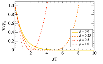
Figure 1: The potential $V(T)$ as a function of the tachyon field $T$ is shown to some $\beta$-values.

For the potential (13), the slow-roll parameters is

$$\varepsilon_{1}(T)=\dfrac{M_{p}^{2}\lambda^{2}}{2\alpha^{\prime}V_{0}}\left(1-\beta\lambda T\right)^{-2-1/\beta},\qquad\varepsilon_{2}(T)=\dfrac{M_{p}^{2}\lambda^{2}(1-2\beta)}{\alpha^{\prime}V_{0}}\left(1-\beta\lambda T\right)^{-2-1/\beta},$$ (14)

while the scalar spectral index and the tensor-to-scalar ratio are given by

$$n_{s}=1-\dfrac{2M_{p}^{2}\lambda^{2}}{\alpha^{\prime}V_{0}}(1+\beta)\left(1-\beta\lambda T\right)^{-2-1/\beta},\quad r=\dfrac{8M_{p}^{2}\lambda^{2}}{\alpha^{\prime}V_{0}}\left(1-\beta\lambda T\right)^{-2-1/\beta}.$$ (15)

On the other hand, through Eq. (12), it is straightforward to obtain the number of e-folds,

$$N=\dfrac{\alpha^{\prime}V_{0}}{M_{p}^{2}\lambda^{2}(1+2\beta)}\left[\left(1-\beta\lambda T_{k}\right)^{2+1/\beta}-\left(1-\beta\lambda T_{e}\right)^{2+1/\beta}\right],$$ (16)

where $T_{e}$ is the value of $T$ when inflation ends, i.e., $\varepsilon_{1}(T_{e})=1\Rightarrow\left(1-\beta\lambda T_{e}\right)^{2+1/\beta}=M_{p}^{2}\lambda^{2}/2\alpha^{\prime}V_{0}$, then

$$\left(1-\beta\lambda T_{k}\right)^{2+1/\beta}=\dfrac{M_{p}^{2}\lambda^{2}}{2\alpha^{\prime}V_{0}}\left[1+2N(1+2\beta)\right].$$ (17)

Therefore, we can rewrite the slow-roll parameters as a function of $N$ as follows:

$$\varepsilon_{1}=\dfrac{1}{1+2N(1+2\beta)},\quad\varepsilon_{2}=\dfrac{2+4\beta}{1+2N(1+2\beta)}.$$ (18)

Now, using (15), we get

$$n_{s}=1-\dfrac{4(1+\beta)}{1+2N(1+2\beta)},\quad r=\dfrac{16}{1+2N(1+2\beta)}.$$ (19)

The $r$ vs. $n_{s}$ plane shown in Fig. 2 presents constraints derived from the Planck 2018 baseline analysis. Additionally, incorporating BK18 & BAO (PLANCK2018, ), one refines and narrows these constraints, which improves the bounds on the primordial gravitational waves parameterized by the tensor-to-scalar ratio $r$. Besides, the inclined thick line divides the $r$ vs. $n_{s}$ plane between convex and concave potentials. So, for values of $\beta<0.8$, the $\beta$-exponential potential behaves as a convex potential otherwise presents a concave shape. Moreover, at $95\%$ CL, from Planck TT,TE,EE+lowE+lensing likelihood, the tachyonic inflation is excluded for $\beta\geq 2.0$ ($\beta\leq 2\times 10^{-2}$) with $N\geq 50$ ($N\leq 60$). On the other hand, in light of the joint Planck Collaboration $2018$ baseline analysis, when adding BK18 & BAO, the $\beta$-exponential tachyonic inflation model is ruled out for any $\beta$-values. Finally, as $\beta$-parameter increases, the tachyonic inflation prediction converges for the $\beta$-exponential standard estimate (SANTOS, ).

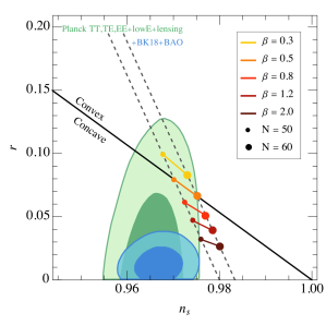
Figure 2: The marginalized joint regions at $68\%$ and $95\%$ confidence levels for the spectral index ($n_{s}$) and tensor-to-scalar ratio ($r$) derived from Planck data both independently and in combination with BK18+BAO data (PLANCK2018, ), compared to the theoretical predictions of the tachyonic inflationary $\beta$-exponential model. The number of e-folds have been fixed at $N=50$ and $N=60$.

In the next subsection, we discuss the semiclassical treatment for this theoretical model aiming to obtain the relation between quantum and classical measurements.

II.2 Semiclassical regime

In the semiclassical gravity approach, in which the matter fields are treated from quantum mechanics perspective, whereas the gravity is studied within a classical framework, we can perform a metric and field perturbations splitting $g_{ab}=g_{ab}^{(0)}+\delta g_{ab}$ and $T(t,\vec{x})=\bar{T}(t)+\delta T(t,\vec{x})$, where $\bar{T}(t)$ is the average background field. We choose to work in the longitudinal gauge, and now focusing on the scalar perturbations at first order, the line element associated to the metric is

$$ds^{2}=-(1+2\Phi)dt^{2}+a^{2}(t)(1-2\Phi)\delta_{ij}dx^{i}dx^{j},$$ (20)

where $\Phi$ represents the scalar perturbation, which in the Newtonian limit is identified with the effective gravitational potential. Using equation (2) with the metric element of longitudinal gauge from equation (20), we find that the perturbed Einstein’s equation $\delta G_{\nu}^{\mu}=8\pi G\delta T_{\nu}^{\mu}$ for tachyon scalar field can be calculated, in Fourier modes, and provides us (SINGH, ):

$$3H^{2}\Phi+3H\dot{\Phi}+\frac{k^{2}\Phi}{a^{2}}=-4\pi G\delta\rho,$$ (21)

$$\ddot{\Phi}+4H\dot{\Phi}+\left(2\dot{H}+3H^{2}\right)\Phi=4\pi G\delta p,$$ (22)

$$\dot{\Phi}+H\Phi=\dfrac{3H^{2}}{2}\alpha^{\prime}\dot{\bar{T}}\delta T,$$ (23)

where

$$\delta\rho =\dfrac{\dot{H}}{4\pi G}\frac{\Phi}{\left(1-\alpha^{\prime}\dot{\bar{T}}^{2}\right)}+\dfrac{3H^{2}}{8\pi G}\frac{\alpha^{\prime}\dot{\bar{T}}\delta\dot{T}}{\left(1-\alpha^{\prime}\dot{\bar{T}}^{2}\right)}+\dfrac{V_{T}\delta T}{\sqrt{1-\alpha^{\prime}\dot{\bar{T}}^{2}}},$$ (24)

$$\delta p =\dfrac{\dot{H}}{4\pi G}\Phi+\dfrac{3H^{2}}{8\pi G}\alpha^{\prime}\dot{\bar{T}}\delta\dot{T}-V_{T}\delta T\sqrt{1-\alpha^{\prime}\dot{\bar{T}}^{2}}.$$ (25)

Combining these equations and performing a change of variables of the time $t$ by the conformal time, $dt=a(\eta)d\eta$, we obtain

$$\Phi_{k}=\sqrt{\dfrac{3\alpha^{\prime}\varepsilon_{1}}{2}}\dfrac{H^{2}}{c_{s}^{2}k^{2}}a\langle\delta\hat{T}^{\prime}\rangle.$$ (26)

This result indicates that when the state is the vacuum, that is $\langle 0|\delta\hat{T}^{\prime}|0\rangle=0$, there are no perturbations at any scale $k$, i.e., $\Phi_{k}=0$. Only after the self-induced collapse of the wave function whose expectation value satisfies $\langle 0|\delta\hat{T}^{\prime}|0\rangle\neq 0$ gives rise to the primordial perturbations.

III Collapse Spontaneous Localization (CSL)

The self-induced collapse hypothesis of the inflaton wave function has been discussed as a likely physical process which leads to the emergence of inhomogeneity and anisotropy (LEON1, ; PICCIRILLI, ; CANATE, ; GLEON, ; LEON, ). In this section, we aim to start the treatment of the quantum theory for the field $\delta\hat{T}$. For this purpose, one can rescale the field variable, $y=z\delta T$, with $z=\sqrt{3\alpha^{\prime}}M_{p}a\dot{\bar{T}}/c_{s}$, expanding the action (1) up to second order in $y$, we find

$$S=\dfrac{1}{2}\int d\eta d^{3}x\left[y^{\prime\,2}-c_{s}^{2}(\partial_{i}y)^{2}-2\dfrac{z^{\prime}}{z}yy^{\prime}+\dfrac{z^{\prime\,2}}{z^{2}}y^{2}\right].$$ (27)

Here, both fields $y$ and the canonical conjugated momentum $\pi=y^{\prime}-(z^{\prime}/z)y=z\delta\hat{T}^{\prime}$ satisfy the commutation relations $[\hat{y}(\eta,\vec{x}),\hat{\pi}(\eta,\vec{x})]=i\delta(\vec{x}-\vec{x}^{\prime})$, $[\hat{y}(\eta,\vec{x}),\hat{y}(\eta,\vec{x}^{\prime})]=[\hat{\pi}(\eta,\vec{x}),\hat{\pi}(\eta,\vec{x})]=0$. From Eq. (27) one can obtain the Hamiltonian

$$H=\dfrac{1}{2}\int d^{3}x\left[\hat{\pi}^{2}\left(\vec{x}\right)+c_{s}^{2}\left(\nabla\hat{y}\left(\vec{x}\right)\right)^{2}+\frac{z^{\prime}}{z}\hat{y}\left(\vec{x}\right)\hat{\pi}\left(\vec{x}\right)\right].$$ (28)

On its turn, the fields can be rewritten in terms of Fourier modes as follows

$$\hat{y}(\vec{x})=\dfrac{1}{(2\pi)^{3/2}}\int d^{3}k\,\hat{y}(\vec{k})e^{i\vec{k}\cdot\vec{x}},\quad\hat{\pi}(\vec{x})=\dfrac{1}{(2\pi)^{3/2}}\int d^{3}k\,\hat{\pi}(\vec{k})e^{i\vec{k}\cdot\vec{x}}.$$ (29)

The Collapse Spontaneous Localization (CSL) model is defined from a non-unitary modification of the Schrödinger equation that induces a wave function collapse towards one of the possible eigenstates of an operator called the collapse operator (PICCIRILLI, ). In this sense, it is convenient to describe the theory in terms of the Hamiltonian of the system in Fourier modes, which in this case is given by

$$\hat{H}_{\vec{k}}^{R,I}=\dfrac{1}{2}\int d^{3}k\left[\hat{\pi}_{\vec{k}}^{R,I}\hat{\pi}_{\vec{k}}^{*R,I}+c_{s}^{2}k^{2}\hat{y}_{\vec{k}}^{R,I}\hat{y}_{\vec{k}}^{*R,I}-\dfrac{(1+\varepsilon_{1}+\varepsilon_{2}/2)}{\eta}\left(\hat{y}_{\vec{k}}^{R,I}\hat{\pi}_{\vec{k}}^{*R,I}+\hat{y}_{\vec{k}}^{*R,I}\hat{\pi}_{\vec{k}}^{R,I}\right)\right],$$ (30)

where the indexes $R$,$I$ denote the real and imaginary parts of $\hat{y}_{\vec{k}}$ and $\hat{\pi}_{\vec{k}}$, respectively. Defining by $\Phi[\pi]$ the wave functional characterizing the quantum state of the field, one can factorize $\Phi[\pi]$ into mode component $\Phi[y_{\vec{k}}]=\Pi_{\vec{k}}\Phi[y_{\vec{k}}^{R}]\,\times\,\Phi[y_{\vec{k}}^{I}]$. Here, we are aiming to deal with each mode separately. Since the Hamiltonian is quadratic in $y_{\vec{k}}^{R,I}$ and $\pi_{\vec{k}}^{R,I}$, is natural to assume a Gaussian state

$$\Phi^{R,I}(\eta,\pi_{\vec{k}}^{R,I})=\exp[-A_{k}(\eta)(\pi_{\vec{k}}^{R,I})^{2}+B_{k}(\eta)\pi_{\vec{k}}^{R,I}+C_{k}(\eta)],$$ (31)

with the wave function evolving according to Schrödinger equation, and satisfying the initial conditions given by $A_{k}(\tau)=1/2k$, $B_{k}(\tau)=C_{k}(\tau)=0$. So, the evolution of the state vector characterizing the inflaton as given by the CSL theory is assumed to be

$$\left|\Phi_{\vec{k}}^{R,I},\eta\right\rangle=\hat{\mathcal{T}}\exp\left\{-\int_{\tau}^{\eta}d\eta^{\prime}\left[i\hat{H}_{\vec{k}}^{R,I}+\dfrac{(\mathcal{W}(\eta^{\prime})-2\lambda_{k}^{2}\hat{\pi}_{\vec{k}}^{R,I})^{2}}{4\lambda_{k}}\right]\right\}\left|\Phi_{\vec{k}}^{R,I},\tau\right\rangle,$$ (32)

where $\hat{\mathcal{T}}$ is the time-ordering operator and $\mathcal{W}\left(\eta^{\prime}\right)$ is the background noise that can be considered as a stochastic process with continuous time. Using the solution (31) and the CSL evolution equations, it can be shown that (CANATE, )

$$\overline{\langle\hat{\pi}_{\vec{k}}^{R,I}\rangle^{2}}=\overline{\langle(\hat{\pi}_{\vec{k}}^{R,I})^{2}\rangle}-\dfrac{1}{4\mbox{Re}{A_{k}(\eta)}}.$$ (33)

Note that $\left(4\mbox{Re}{A_{k}(\eta)}\right)^{-1}$ represents the variance of the momentum operator.

In this point, we can relate this quantity to the scalar power spectrum defined through the relation

$$\overline{\Phi_{\vec{k}}\Phi_{\vec{k}^{\prime}}^{*}}=\dfrac{3\alpha^{\prime}\varepsilon_{1}}{2}\dfrac{a^{2}H^{4}}{z^{2}k^{4}}\overline{\langle\hat{\pi}_{\vec{k}}\rangle\ \langle\hat{\pi}_{\vec{k}^{\prime}}\rangle^{*}}=\frac{2\pi^{2}}{k^{3}}\mathcal{P}_{\Phi}(k)\delta(\vec{k}-\vec{k}),$$ (34)

where $\mathcal{P}_{\Phi}(k)$ is the dimensionless scalar power spectrum, which is related to $\mathcal{P}_{s}(k)$ by (HWANG, )

$$\mathcal{P}_{\Phi}(k)=\frac{H^{2}}{\dot{\bar{T}}^{2}}\mathcal{P}_{s}(k).$$ (35)

On the other hand, admitting that

$$\overline{\langle\hat{\pi}_{\vec{k}}\rangle\ \langle\hat{\pi}_{\vec{k}^{\prime}}\rangle^{*}} =\overline{\langle\hat{\pi}_{\vec{k}}^{R}+i\hat{\pi}_{\vec{k}}^{I}\rangle\ \langle\hat{\pi}_{\vec{k}^{\prime}}^{R}-i\hat{\pi}_{\vec{k}^{\prime}}^{I}\rangle}$$

$$=\left(\overline{\langle\hat{\pi}_{\vec{k}}^{R}\rangle^{2}}+\overline{\langle\hat{\pi}_{\vec{k}}^{I}\rangle^{2}}\right)\delta(\vec{k}-\vec{k}^{\prime}),$$ (36)

we obtain

$$\mathcal{P}_{\Phi}(k) = \dfrac{3\alpha^{\prime}\varepsilon_{1}}{4\pi^{2}}\dfrac{a^{2}H^{4}}{z^{2}}\dfrac{\left(\overline{\langle\hat{\pi}_{\vec{k}}^{R}\rangle^{2}}+\overline{\langle\hat{\pi}_{\vec{k}}^{I}\rangle^{2}}\right)}{k}$$ (37)

$$= \dfrac{3\alpha^{\prime}c_{s}^{2}H^{4}}{8\pi^{2}M_{p}^{2}}\dfrac{\left(\overline{\langle\hat{\pi}_{\vec{k}}^{R}\rangle^{2}}+\overline{\langle\hat{\pi}_{\vec{k}}^{I}\rangle^{2}}\right)}{k},$$

in which the relation $z=\sqrt{3\alpha^{\prime}}M_{p}a\dot{\bar{T}}/c_{s}$ was used. Furthermore, the expected value in (33) is straightforward obtained by assuming that wave function have the form (31),

$$\overline{\langle(\pi_{\vec{k}}^{R,I})^{2}\rangle} \simeq \frac{c_{s}k}{\pi}2^{2\nu_{s}-2}\Gamma^{2}(\nu_{s})\left[1+\lambda_{k}\sin\gamma_{k}\cos\gamma_{k}\right.$$ (38)

$$- \left.\frac{\lambda_{k}c_{s}k\tau}{2}\left(\frac{3}{\nu_{s}+1}\sin^{2}\gamma_{k}+\frac{\cos^{2}\gamma_{k}}{\nu_{s}}\right)\right](-c_{s}k\eta)^{-2\nu_{s}+1},$$

with $\gamma_{k}\equiv-c_{s}k\tau-\nu_{s}\pi/2-3\pi/4$. On its turn, the second term of r.h.s. in (33) is given by

$$\dfrac{1}{4\mbox{Re}{[A_{k}(\eta)]}}\simeq\frac{c_{s}k2^{2\nu_{s}-2}\zeta_{k}^{-2\nu_{s}}\sin(\pi\nu_{s})\Gamma^{2}(\nu_{s})(-c_{s}k\eta)^{-2\nu_{s}+1}}{\pi\sin(2\nu_{s}\theta_{k}+\pi\nu_{s})},$$ (39)

in which $\zeta_{k}\equiv(1+4\lambda_{k}^{2})^{1/4},$ and $\theta_{k}\equiv-1/2\arctan(2\lambda_{k})$ (GLEON, ).

Finally, substituting Eqs. (33), (38), and (39) into (37), we get

$$\mathcal{P}_{\Phi}(k)=\dfrac{3\alpha^{\prime}H^{4}}{4\pi^{2}M_{p}^{2}c_{s}}2^{2\nu_{s}-2}\Gamma^{2}(\nu_{s})(-c_{s}k\eta)^{-2\nu_{s}+1}\mathcal{F}(\lambda_{k},\nu_{s}),$$ (40)

where $\mathcal{F}(\lambda_{k},\nu_{s})$ is a function of collapse parameter, given by

$$\mathcal{F}(\lambda_{k},\nu_{s}) =1+\lambda_{k}\sin\gamma_{k}\cos\gamma_{k}-\dfrac{\lambda_{k}c_{s}k\tau}{2}\left(\dfrac{3}{\nu_{s}+1}\sin^{2}\gamma_{k}+\dfrac{\cos^{2}\gamma_{k}}{\nu_{s}}\right)$$

$$-\dfrac{\sin(\pi\nu_{s})}{\zeta_{k}^{2\nu_{s}}\sin(2\nu_{s}\theta_{k}+\pi\nu_{s})}.$$ (41)

Now, from Eqs. (35) and (40) we can identify $\mathcal{P}_{s}(k)$ as follows:

$$\mathcal{P}_{s}(k)=\mathcal{A}_{s}(k)\mathcal{F}(\lambda_{k},\nu_{s}),$$ (42)

where $\mathcal{A}_{s}$ is the amplitude of scalar power spectrum, given by (DBAUMANN, )

$$\mathcal{A}_{s}=\frac{H^{2}}{8\pi^{2}M_{p}^{2}c_{s}\varepsilon_{1}}\,\mbox{.}$$ (43)

On the other hand, for tensor perturbations, as shown in (GLEON, ), the tensor collapse function is analogous to scalar collapse function, and therefore

$$\mathcal{P}_{t}(k)=\mathcal{A}_{t}(k)\mathcal{F}(\lambda_{k},\nu_{t}),$$ (44)

where $\nu_{t}=1/2+\varepsilon_{1}$ and the amplitude of tensor power spectrum is given by (DBAUMANN, )

$$\mathcal{A}_{t}=\frac{2H^{2}}{\pi^{2}M_{p}^{2}}.$$ (45)

Therefore, these results indicate that the collapse parameter $\lambda_{k}$ modifies the behavior of the power spectrum, and such deviations, eventually, can be measured in experiments of the Cosmic Microwave Background (CMB) spectrum, for instance. Furthermore, it has been showed that when $\lambda_{k}=\lambda_{0}/c_{s}k$, the primordial power spectrum becomes nearly scale-invariant (LEON, ). This leads to define

$$\lambda_{k}\equiv\lambda_{0}\left(\dfrac{1}{c_{s}k}+\dfrac{\alpha}{c_{s}^{2}k^{2}}\right),$$ (46)

where $\lambda_{0}=1/\left|\tau\right|\simeq 6.41\times 10^{-9}\mathrm{Mpc^{-1}}$, and the extra added parameter $\alpha$ will account for the effects from CSL model. Moreover, recent works have pointed out that the additional term $\alpha/c_{s}^{2}k^{2}$ induces similar estimates as a standard $\Lambda$CDM model (MICOL, ).

IV Power spectrum constraints from the CSL scheme

In this section, we aim to analyze the deviations produced by the collapse parameter from CSL theory on the scalar power spectrum. Thus, by using the $\beta$-exponential potential (13), and (17) we can rewrite (42) as

$$\mathcal{P}_{s}=\dfrac{\lambda^{2/(2\beta+1)}}{24}\left(\frac{V_{0}}{\pi^{2}M_{p}^{4}}\right)^{\frac{2\beta}{2\beta+1}}\left[1+2N(1-2\beta)\right]^{\frac{2\beta+2}{2\beta+1}}\mathcal{F}(\lambda_{k},\nu_{s}).$$ (47)

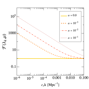
Figure 3: In the context of the CSL inflationary model, the function $\mathcal{F}(\lambda_{k},\nu_{s})$ is associated with the power spectrum. The parameters $\lambda_{0}$ (set at $1/\left|\tau\right|=6.41\times 10^{-9}\mathrm{Mpc^{-1}}$) and $\mu$ (fixed at 0.5), remain constant.

Recent analysis, assuming that $\lambda_{k}$ must be positive, has imposed constraints on $\alpha$-parameter such that $\alpha>-10^{-6}$ for the relevant $c_{s}k$ values (PICCIRILLI, ). Therefore, replacing Eq. (46) in (41) – for small values of $\alpha$ – one may now expand the collapse function in first order on the $\alpha$-parameter, such that the function of the collapse parameter becomes

$$\mathcal{F}(\lambda_{k},\mu)\simeq 1+B(c_{s}k,\mu)\alpha,$$ (48)

in which $\mu=\nu_{s},\nu_{t}$ and the function $B(c_{s}k,\mu)$ is given by

$$B(c_{s}k,\mu) = \frac{\lambda_{0}}{c_{s}^{2}k^{2}}\sin\gamma_{k}\cos\gamma_{k}-\frac{\lambda_{0}\tau}{2c_{s}k}\left(\dfrac{3}{\mu+1}\sin^{2}\gamma_{k}+\dfrac{\cos^{2}\gamma_{k}}{\mu}\right)$$ (49)

$$- \frac{4\mu\lambda_{0}^{2}}{c_{s}^{3}k^{3}(1+4\lambda_{0}^{2}/c_{s}^{2}k^{2})^{1+\mu/2}}\frac{\sin(\pi\mu)}{\sin(\mu\arctan(2\lambda_{0}/c_{s}k)-\pi\mu)}$$

$$- \frac{2\mu\lambda_{0}}{c_{s}^{2}k^{2}(1+4\lambda_{0}^{2}/c_{s}^{2}k^{2})^{1+\mu/2}}\frac{\sin(\pi\mu)\cos(\mu\arctan(2\lambda_{0}/c_{s}k)-\pi\mu)}{\sin^{2}(\mu\arctan(2\lambda_{0}/c_{s}k)-\pi\mu)}\mbox{.}$$

Noteworthy is that, for $\alpha=0$, then $\mathcal{F}(\lambda_{0},\nu_{s})=\mathcal{F}(\lambda_{0},\nu_{t})=1$, and there is no modification on the standard shape of the power spectrum. Moreover, the different values of $\alpha$ change the behavior of $\mathcal{P}_{s}$ and $\mathcal{P}_{t}$, which implies modifications in the spectral index of the inflation. In Fig. 3 we present the plot of the function of collapse parameter, $\mathcal{F}(\lambda_{k},\nu_{s})$, for different values of $\alpha$. We note that at lower values of $k$, the standard primordial power spectrum shape ($\alpha=0$) differs significantly from the spectrum produced by the CSL collapse model.

On its turn, the spectral index $n_{s}$ is defined by the relation

$$n_{s}-1\equiv\frac{d\ln\mathcal{P}_{s}}{d\ln k}=\frac{d\ln\mathcal{A}_{s}}{d\ln k}+\frac{d\ln\mathcal{F}(\lambda_{k},\nu_{s})}{d\ln k}\,\mbox{,}$$ (50)

whereas, on the one hand, we have

$$\frac{d\ln\mathcal{A}_{s}}{d\ln k}=-2\varepsilon_{1}-\varepsilon_{2}\,\mbox{,}$$ (51)

and, on the other hand, the variation of the collapse function satisfies

$$\frac{d\ln\mathcal{F}(\lambda_{k},\nu_{s})}{d\ln k}=-\frac{1}{1-\varepsilon_{1}}\frac{M_{p}^{2}V_{T}}{\alpha^{\prime}V^{2}}\frac{d\nu_{s}}{dT}\frac{d\ln\mathcal{F}(\lambda_{k},\nu_{s})}{d\nu_{s}}\,\mbox{.}$$ (52)

So, given that $\nu_{s}=1/2+\varepsilon_{1}+\varepsilon_{2}/2$, we obtain

$$\frac{M_{p}^{2}V_{T}}{\alpha^{\prime}V^{2}}\frac{d\nu_{s}}{dT}\simeq-\varepsilon_{1}\varepsilon_{2}-\varepsilon_{1}\varepsilon_{3}\mbox{,}$$ (53)

while

$$\frac{d\ln\mathcal{F}(\lambda_{k},\nu_{s})}{d\nu_{s}}\simeq\alpha\frac{dB(c_{s}k,\nu_{s})}{d\nu_{s}}\approx\alpha\left[K_{0}+K_{1}f(\varepsilon_{1},\varepsilon_{2})\right]\,\mbox{,}$$ (54)

in which $K_{0}\equiv K_{0}(c_{s}k)$, $K_{1}\equiv K_{1}(c_{s}k)$, and $f(\varepsilon_{1},\varepsilon_{2})=\varepsilon_{1}+\varepsilon_{2}/2$, such that

$$K_{0}(c_{s}k) =-\frac{\lambda_{0}\pi\left(2\sin(-2c_{s}k\tau)+\pi\cos(-2c_{s}k\tau)\right)}{4c_{s}^{2}k^{2}}+\frac{2\lambda_{0}\tau\left(\sin^{2}(-c_{s}k\tau)+3\cos^{2}(-c_{s}k\tau)\right)}{3c_{s}k}$$

$$+\frac{\lambda_{0}\pi\ln B\left[c_{s}k+2\lambda_{0}(C-\pi)(\ln B-2)\right]}{c_{s}^{3}k^{3}B(C-\pi)^{2}},$$ (55)

$$K_{1}(c_{s}k) =-\frac{\lambda_{0}\pi^{2}\tau}{c_{s}^{2}k^{2}}+\frac{8\lambda_{0}\tau}{9c_{s}k}\left(1+8\cos^{2}(-c_{s}k\tau)+3\pi\sin(-c_{s}k\tau)\cos(-c_{s}k\tau)\right)$$

$$+\frac{4\pi\lambda_{0}^{2}\ln B}{c_{s}^{3}k^{3}B(C-\pi)}+\frac{\lambda_{0}\pi\left(4C^{2}-8C\pi-3\ln^{2}B+8\pi^{2}\right)}{6c_{s}^{2}k^{2}B(C-\pi)^{2}},$$ (56)

where $B=1+4\lambda_{0}^{2}/c_{s}^{2}k^{2}$, and $C=\arctan\left(2\lambda_{0}/c_{s}k\right)$. The functions $K_{i}$ ($i=0,1$) are obtained by expanding the first order derivative on the slow-roll parameters. Therefore, considering an approximation to second order in the slow-roll parameters, we obtain

$$n_{s}=1-2\varepsilon_{1}-\varepsilon_{2}+K_{0}(\varepsilon_{1}\varepsilon_{2}+\varepsilon_{1}\varepsilon_{3})\alpha,$$ (57)

where, for a pivot scale value $c_{s}k=0.002\,\mbox{Mpc}^{-1}$, $\tau=-10^{8}\mbox{Mpc}^{-1}$, and $\lambda_{0}=6.51\times 10^{-9}\mbox{Mpc}^{-1}$, we get $K_{0}=-648.78\mbox{Mpc}^{-1}$.

On its turn, for the ratio of tensor-to-scalar fluctuations, becomes

$$r\equiv\frac{\mathcal{P}_{t}}{\mathcal{P}_{s}}=\frac{\mathcal{A}_{t}}{\mathcal{A}_{s}}\frac{\mathcal{F}(\lambda_{k},\nu_{t})}{\mathcal{F}(\lambda_{k},\nu_{s})}\mbox{.}$$ (58)

Using the definitions $\nu_{s}=1/2+\varepsilon_{1}+\varepsilon_{2}/2$ and $\nu_{t}=1/2+\varepsilon_{1}$ and approximating in first order on slow-roll parameters, we obtain

$$r=16\varepsilon_{1}\left(1+\alpha K_{2}\varepsilon_{2}\right)\mbox{,}$$ (59)

with

$$K_{2}(c_{s}k) =-\frac{\lambda_{0}\pi}{4c_{s}^{2}k^{2}}\sin(-2c_{s}k\tau)-\frac{2\lambda_{0}\tau}{3c_{s}k}\left(2+\cos(-2c_{s}k\tau)\right)+\frac{2\pi\lambda_{0}^{2}}{c_{s}^{3}k^{3}B(C-\pi)}$$

$$-\frac{\lambda_{0}\pi\ln B}{2c_{s}^{2}k^{2}B(C-\pi)^{2}},$$ (60)

where $K_{2}=\left.\left(B(c_{s}k,\nu_{t})-B(c_{s}k,\nu_{s})\right)\right|_{c_{s}k=0.002}=1297.57\mbox{Mpc}^{-1}$, for $\tau=-10^{8}\mbox{Mpc}^{-1}$ and $\lambda_{0}=6.51\times 10^{-9}\mbox{Mpc}^{-1}$. Furthermore, we can verify that when turning off the CSL collapse model effects, i.e., we take $\alpha=0$, relations (57) and (59) recover the standard value, as expected.

Finally, with these results, by considering the $\beta$-exponential potential, we get the scalar spectral index and tensor-to-scalar ratio, as follows

$$n_{s} = 1-\frac{4(1+\beta)}{1+2N(1+2\beta)}+\frac{6K_{0}(1+2\beta)}{[1+2N(1+2\beta)]^{2}}\alpha,$$ (61)

$$r = \frac{16}{1+2N(1+2\beta)}+\frac{2K_{2}(1+2\beta)}{[1+2N(1+2\beta)]^{2}}\alpha.$$ (62)

The deviations owing to the collapse parameter are shown in the $n_{s}-r$ plane (Fig. 4). The constraints shown in Fig. 4 for the Planck 2018 baseline analysis, adapted from (PLANCK2018, ), incorporating BICEP/Keck along with BAO data, present bounds that exclude the tachyonic $\beta$-exponential inflation in the CSL approach on determined ranges of $\alpha$ and $\beta$ parameters. In this case, the contours in the vertical ($r$) direction are shrunk by the BK18 data, whereas the BAO data shrinks the contours along the horizontal ($n_{s}$) direction (PLANCK2018, ). At $95\%$ CL, from Planck TT,TE,EE+lowE+lensing likelihood, for $N=50$, the results impose bounds on the collapse parameter such that $\alpha<2.0\times 10^{-1}\,\mathrm{Mpc^{-1}}$, for $\beta=1.6$. Furthermore, from this analysis, one can observe that, for $N=60$, we must have $\alpha<7.0\times 10^{-2}\,\mathrm{Mpc^{-1}}$ with $\beta=0.6$.

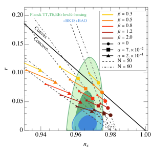
Figure 4: The $n_{s}-r$ plane for the $\beta$-exponential potential is shown for different values of $\alpha$ and $\beta$. The standard tachyon inflation is recovered by assuming $\alpha=0$, while $\alpha\neq 0$ introduces the CSL inflationary model deviations, which changes the behavior of the standard spectral index. Two values for the number of e-folds, $N=50$ (dashed lines) and $N=60$ (dash-dotted curves), are considered.

On the other hand, the constraint for Planck measurements (BK15) (PLANCK, ) indicates that, for $N=50$, we have $\alpha=0.036\,\mbox{Mpc}^{-1}$ and $\beta=0.688$, from the spectral index (61) and the tensor-to-scalar ratio (62), for $n_{s}=0.9658$ and $r=0.071$. In its turn, this analysis also allows us to impose bounds on the $\beta$-parameter as long as we keep the collapse parameter fixed. Indeed, in the case in which $\alpha=7.0\times 10^{-2}\,\mathrm{Mpc^{-1}}$, for $N\geq 50$, so $\beta\lesssim 6$, while for $\alpha=2.0\times 10^{-1}\,\mathrm{Mpc^{-1}}$, we find that $\beta\lesssim 11$ (for $N\geq 50$). These results show the relationship between the $\alpha$-parameter and the other free parameters of the $\beta$-exponential potential. As we saw, the CSL approach weakens the constraints on the $\beta$-exponential model, although it provides an excellent agreement between the theoretical estimate and the current observational data. Finally, it is worth mentioning that even by adding the BK18 & BAO data to the Planck Collaboration $2018$ baseline analysis, we can not rule out the inflation tachyon $\beta$-exponential model in the CSL scheme for a large scale of the $\alpha$- and $\beta$-parameters.

V Concluding Remarks

In this work, we have analyzed phenomenologically the constraints on the collapse parameter, $\alpha$, by considering the tachyonic inflationary $\beta$-exponential model in the context of the CSL approach. Initially, we obtained constrained values for the standard $\beta$-exponential model so that for $N\geq 50$ ($N\leq 60$), we must have $\beta\leq 2.0$ ($\beta\geq 2\times 10^{-2}$). Performing a semiclassical treatment, we find the relation between quantum measurements to the classical perturbations, and using the CSL model, we have obtained an important modification in both the amplitude and shape of the primordial power spectrum, which presents dependence on the strength of the collapse parameter, $\alpha$. We show that if one turns off the quantum effects owing to the collapse parameter, i.e., when $\alpha=0$, one recovers the expected result from tachyonic inflation.

Finally, the modifications owing to the CSL scheme, when applied to the $\beta$-exponential potential, lead to deviations in the spectral indexes, which, in principle, could yield a clear fingerprint of tachyonic inflation on the CMB spectrum. From this analysis, we were able to impose bounds on the collapse parameter. Indeed, for a realistic number of e-folds before the end of inflation, i.e., $N=50\left(60\right)$, and for $\beta=1.6\left(0.6\right)$, one obtains that $\alpha<2.0\times 10^{-1}\,\mathrm{Mpc^{-1}}\left(7.0\times 10^{-2}\,\mathrm{Mpc^{-1}}\right)$. On the other hand, by considering the CSL approach, we have shown that the constraints on the $\beta$-parameter become weak. Indeed, if $\alpha=7.0\times 10^{-2}\,\mathrm{Mpc^{-1}}$ $\left(N\geq 50\right)$, so we must have $\beta\lesssim 6$, whereas for $\alpha=2.0\times 10^{-1}\,\mathrm{Mpc^{-1}}$ $\left(N\geq 50\right)$, we find $\beta\lesssim 11$ . As we see, this study opens an avenue to investigate inflation from other tachyonic potentials by considering the context of the CSL scheme, aiming to obtain new constraints on the collapse parameter.