SymTFTs for Continuous non-Abelian Symmetries

Abstract

Topological defects and operators give a far-reaching generalization of symmetries of quantum fields. An auxiliary topological field theory in one dimension higher than the QFT of interest, known as the SymTFT, provides a natural way for capturing such operators. This gives a new perspective on several applications of symmetries, but fails to capture continuous non-Abelian symmetries. The main aim of this work is to fill this gap. Guided by geometric engineering and holography, we recover various known features of representation theory of the non-Abelian symmetry from a SymTFT viewpoint. Central to our approach is a duality between (flat) free Yang-Mills and non-Abelian BF theories. Our results extend naturally to models without supersymmetry.

I Introduction and motivation

In recent years our understanding of symmetries of quantum field theories (QFTs) has undergone a revolution based on the idea that symmetries are encoded in topological subsectors of the spectrum of QFT operators [1]. While ordinary symmetries are described by groups, symmetries characterized by topological operators have a higher structure that generalizes the notion of group multiplication, believed to be inscribed in a symmetry (higher) category (see e.g. [2, 3, 4, 5, 6, 7, 8, 9] for recent reviews). A very convenient way to characterise generalized finite symmetries of a $d$-dimensional QFT, denoted $\mathbf{T}$, is given by the topological symmetry theory construction (or SymTFT for short) [10, 11, 12, 13] (see also [14, 15, 16, 17, 18, 19, 20, 21, 22, 23, 24, 25, 26, 27, 28, 29]). The construction is based on four ingredients: (1) a $d$-dimensional field theory $\widehat{\mathbf{T}}$ defined relative to (2) a bulk $d+1$ topological field theory $\mathbf{S}$, together with (3) a topological gapped $d$-dimensional boundary condition for $\mathbf{S}$, that we denote $\mathbf{B}$ such that there is (4) an isomorphism of field theories

$$\begin{gathered}\scalebox{0.5}{ \leavevmode\hbox to247.73pt{\vbox to86.56pt{\text{[drawing]}}}}\end{gathered}\;\;. \mathbf{B} \widehat{\mathbf{T}} \mathbf{S} \simeq \mathbf{T} \mathbf{B} \widehat{\mathbf{T}} \mathbf{S} \simeq \mathbf{T}$$ (1)

Schematically, one can encode the topological operators of $\mathbf{T}$ in the topological operators of $\mathbf{S}$ that are non-zero along $\mathbf{B}$. Dually, $\mathbf{B}$ captures background configurations for the symmetry of $\mathbf{T}$, which is gauged in the bulk (where only the Drinfeld center of the symmetry is manifest).

While this construction is very effective for (generalized) finite symmetries, it fails to reproduce verbatim the case of continuous global symmetries for $\mathbf{T}$. The main reason is that while gauging a finite symmetry is a topological operation that can be encoded in a topological boundary changing interface of $\mathbf{S}$, in the case of continuous symmetries the gauging operation is more involved. Gauging a continuous symmetry introduces new degrees of freedom in the spectrum (the gauge mediators as well as various topological solitons) that cannot be captured by a simple topological manipulation on $\mathbf{T}$. Recent proposals in the literature address this topic [30, 31] advancing a SymTFT for continuous $U(1)$ symmetries and conjecturing a possible generalization for continuous non-Abelian symmetries in terms of a non-Abelian version of BF theory. From this latter perspective, however, it is unclear how the representation theory of the non-Abelian flavor symmetry is realized as a bulk-boundary system.

In this letter we give a dual formulation of the topological symmetry theory in terms of free non-Abelian Yang-Mills theory, that allows to address this open question among others.

Our proposal is realized explicitly in the context of geometric engineering as well as in holography, that serve as examples. We stress that the structure which is responsible for capturing the symmetry is the LHS of the diagram in Equation (1), namely the data (2) and (3) in the SymTFT construction, that are completely independent from the choices of $\mathbf{T}$ as well as $\widehat{\mathbf{T}}$:

$$\begin{gathered}\scalebox{0.5}{ \leavevmode\hbox to159.53pt{\vbox to86.56pt{\text{[drawing]}}}}\end{gathered}\;\;. \mathbf{B} \mathbf{S} \mathbf{B} \mathbf{S}$$ (2)

Here we exploit the extra features (such as superconformal invariance) as a strategy for obtaining an explicit expression for $\mathbf{S}$. By the above argument, these extras are not strictly necessary, and indeed our construction holds for non-supersymmetric theories as well .

This note is organized as follows. In Section II we derive the duality between the Horowitz non-Abelian BF theory [33] and free Yang-Mills theory. In Section III we discuss the evidence for our proposal. Our main classes of examples are SCFTs realized via geometric engineering in M-theory, discussed in §.III.1, as well as holographic SCFTs, discussed in §.III.2. In particular, our argument applies uniformly to all holographic SCFTs of $d\geq 4$, as expected since $d+1=4$ is a critical dimension for gravitational theories in AdS. Our analysis of free Yang-Mills as a SymTFT for continuous non-Abelian symmetries is complemented by a first series of applications discussed in Section IV, where we discuss how to recover the representation theory of non-Abelian Lie groups from the bulk-boundary perspective . We present some conclusions and directions of further study in Section V.

Note Added. We were informed by Fabio Apruzzi of an upcoming work [35] that has some overlap with the results in our note.

II SymTFT for continuous non-Abelian symmetries

Motivated by geometric engineering in string theory and holography as discussed in Section III below, we propose that the SymTFT for a QFT in $d$-dimensions with a continuous non-Abelian symmetry of type $G$ contains a $(d+1)$-dimensional free Yang-Mills theory, namely a Yang-Mills theory at zero gauge coupling $g\to 0$. Our claim might seem in tension with the recent proposal by [30, 31] that the relevant SymTFT is the non-Abelian Horowitz BF theory. In this Section we briefly outline a duality of free Yang-Mills with the Horowitz non-Abelian BF theory thus reconciling our proposals.

Following Witten (see e.g. [36], sec. 4.2), one can re-write the Yang-Mills action as follows:

$$\mathbf{S}\supset-{1\over 2g^{2}}\int_{M_{d+1}}\text{tr}\left(f_{2}\wedge\ast f_{2}\right)$$ (3)

$$=\int_{M_{d+1}}\bigg{[}\text{tr}\left(f_{2}\wedge h_{d-1}\right)-\frac{g^{2}}{2}\text{tr}\left(h_{d-1}\wedge\ast h_{d-1}\right)\bigg{]}\ ,$$

where $h_{d-1}$ is a collection of Lagrange multiplier $(d-1)$-form fields transforming in the adjoint of $\mathfrak{g}$.

The corresponding equation of motion is valued in the adjoint of $\mathfrak{g}$ and gives $f_{2}=g^{2}\ast h_{d-1}$. Motivated by geometric engineering and holography, to obtain the contribution to the symmetry theory we need to take the limit $g^{2}\to 0$ of the action above, in particular this implies only the flat connections contribute to the symmetry theory.

By the Ambrose-Singer theorem, all the holonomies of such gauge fields are topological operators, hence we expect to have topological operators corresponding to the Wilson lines of $\mathfrak{g}$ Yang-Mills.

In the $g\to 0$ limit, we obtain the action

$$\int_{M_{d+1}}\text{tr}\left(f_{2}\wedge h_{d-1}\right)\ ,$$ (4)

which is exactly the non-Abelian Horowitz BF theory [33]. In the original action (3), the $(d-1)$-form $h_{d-1}$ has no gauge redundancy, but in (4) $h_{d-1}$ acquires a gauge redundancy,

$$h_{d-1}\sim h_{d-1}+D\lambda_{d}\ ,$$ (5)

where $D$ is the exterior covariant derivative in the adjoint representation. The topological action (4) is invariant under (5) by virtue of the Bianchi identity $Df_{2}=0$.

As already pointed out in [30, 31], from the perspective of non-Abelian BF theory one would like to define holonomies for the Wilson surfaces of $h_{d-1}$, but there is not a good notion of such “surface ordered” integrals. Here our duality with YM at zero coupling is key, since we know that the latter theory has Gukov-Witten operators, which are codimension 2 in the bulk symmetry theory, and become topological as well in the limit of zero coupling. At zero-coupling one can use the description of the Gukov-Witten operators in terms of the dual fluxes for the Cartan subalgebra of the gauge group modulo Weyl [37, 38]. In particular, from this dual perspective, the GW operators in the bulk give rise to a non-invertible subalgebra of the spectrum of the SymTFT for non-Abelian symmetries.

III Evidence from geometric engineering and holography

In this section we discuss evidence for our claim arising from geometric engineering examples (§.III.1), as well as holographic SCFTs (§.III.2).

III.1 SymTFT from Geometry

For the sake of brevity, in this letter we consider the simplest possible geometric engineering scenario, where a $d$-dimensional SCFT is obtained by geometric engineering M-theory on a conical Calabi-Yau singularity $X$ with metric

$$ds^{2}_{X}=dr^{2}+r^{2}ds^{2}_{L_{X}}\ ,$$ (6)

where $L_{X}$ is a Sasaki-Einstein manifold, also known as the link of the singularity. We use this class of geometries here as a main source of examples, but we stress that our results are more general . As a example consider the case $X$ is an orbifold of $\mathbb{C}^{n}$, $\mathbb{C}^{n}/\Gamma$, where $\Gamma$ is a finite subgroup of $SU(n)$ preserving the Calabi-Yau structure. In these cases, the link is a lens space which has at worse orbifold singularities $L_{X}=\mathbb{S}^{2n-1}/\Gamma$. Many examples of $d$-dimensional SCFTs are obtained in this way, in particular choosing $n=3$, one obtains the 5d orbifold SCFTs from M-theory [40, 41].

The geometric origin of the SymTFT for finite symmetries in these cases is encoded in a “geometric engineering limit at infinity”, where the topological operators of $\mathbf{S}$ have a geometric origin as membranes wrapped on torsional cycles of $L_{X}$ [12, 42, 43, 44, 45, 46, 47, 48, 49, 50, 51, 52, 53, 54, 55] building on [56, 57, 58, 59, 60]. The case of continuous symmetries deserve a special analysis. In many cases, continuous symmetries are realized in geometry as non-compact curves of singularities, that intersect the singular locus where the SCFT is located (see e.g. [61, 62, 63, 64, 65, 66, 67, 68, 69, 70, 71] for some examples in various spacetime dimensions). More precisely, consider the case of continuous non-Abelian 0-form symmetries, that arise from non-compact loci of du-Val singularities (split or non-split corresponding to simply-laced vs non-simply laced groups). Since these non-compact loci extend at infinity, the resulting link $L_{X}$ is also singular, with compact loci $C_{\mathfrak{g}_{i}}\subset L_{X}$ of du-Val singularities. The latter correspond to gauge theories in one higher dimension, with gauge couplings $1/g^{2}_{i}\sim\text{vol }(C_{\mathfrak{g}_{i}})$. However, since the link is at infinity in geometry, all of its compact cycles have infinite volume in the metric (6), hence the corresponding higher dimensional gauge theory contributes to the SymTFT only in the limit $g^{2}_{i}\to 0$. To capture the contribution to the symmetry theory from the singularity link we can follow the procedure outlined in the previous section for each of these factors, obtaining the action

$$\int_{M_{d+1}}\text{tr}\left(f_{2,i}\wedge h_{d-1,i}\right)\ .$$ (7)

An explicit example: 5d $T_{N}$ SCFTs. The 5d $T_{N}$ theory is obtained geometrically engineering M-theory on the orbifold $X_{N}=\mathbb{C}^{3}/(\mathbb{Z}_{N}\times\mathbb{Z}_{N})$ where the action by $\mathbb{Z}_{N}\times\mathbb{Z}_{N}$ is $(z_{1},z_{2},z_{3})\to(\alpha z_{1},\overline{\alpha}\beta z_{2},\overline{\beta}z_{3})$ and $\alpha^{N}=\beta^{N}=1$ [61]. In this case the three curves $C_{1}\colon z_{2}=z_{3}=0$, $C_{2}\colon z_{1}=z_{3}=0$ and $C_{3}\colon z_{1}=z_{2}=0$ correspond to three different non-compact loci of $\mathbb{C}^{2}/\mathbb{Z}_{N}$ singularities, associated to the 0-form symmetry $SU(N)^{3}$ of this theory. Consider the link of this singularity, one obtains $L_{X}=\mathbb{S}^{5}/(\mathbb{Z}_{N}\times\mathbb{Z}_{N})\,,$ where the $\mathbb{S}^{5}$ has equation $|z_{1}|^{2}+|z_{2}|^{2}+|z_{3}|^{2}=R^{2}$ and the limit $R\to\infty$ is taken in the metric.

Each of the three curves of singularities in $X_{N}$, corresponds to a singular locus on $L_{X}$, $C_{i}\,\longleftrightarrow\,z_{i}\bar{z}_{i}=R^{2}$, which is an $S^{1}$ with radius $R$.

The reduction of M-theory on $S^{1}\times\mathbb{C}^{2}/\mathbb{Z}_{N}$ correspond to a 6d dynamical $\mathfrak{su}_{N}$ field theory with gauge coupling ${1\over g^{2}}\sim R$. In the spirit of the geometric engineering at infinity origin of the SymTFT, it is tempting to conclude that each of these fixed loci contributes one such gauge theory sector. However, one has to keep track of the fact that the link of the singularity in the metric (6) is of infinite size. Hence, we need to take the limit $R\to\infty$ in the analysis above, which is a limit of zero gauge coupling. To capture the contribution to the symmetry theory from the singularity link, then by the steps outlined above we obtain $\sum_{i=1}^{3}\int_{M_{6}}\text{tr}\left(f_{2,i}\wedge h_{4,i}\right)$, as expected.

III.2 SymTFT from Holography

In this section we confirm our main result for those CFTs in $d\geq 4$ dimensions with a continuous non-Abelian 0-form symmetry $G$ that have a holographic dual in $AdS_{d+1}$ . In AdS/CFT the usual interpretation is that the holographic dual of a global symmetry is indeed a gauge symmetry in the bulk [73]. In particular, the $AdS_{d+1}$ low-energy action contains a Yang-Mills term

$$S_{\rm YM}=-\frac{1}{2g^{2}}\int_{AdS_{d+1}}{\rm tr}(f_{2}\wedge*f_{2})\ ,$$ (8)

as well as other interactions, depending on the model. To capture the holographic dual of the topological symmetry theory we consider an asymptotic limit of the bulk gravitational theory, focusing on the region close to the AdS boundary where only a topological sector of the bulk theory survives . We want to estimate the effect of the Yang-Mills term near the conformal boundary of $AdS_{d+1}$. We work in a fixed pure $AdS_{d+1}$ background. The metric is conformally flat,

$$ds^{2}_{AdS_{d+1}}=\frac{L^{2}}{z^{2}}d\widetilde{s}^{2}_{d+1}\ ,\quad d\widetilde{s}^{2}_{d+1}=dz^{2}+ds^{2}_{\mathbb{R}^{1,d-1}}\ ,$$ (9)

with $L$ the $AdS_{d+1}$ radius and the conformal boundary located at $z=0$. We can write the Yang-Mills term as

$$S_{\rm YM}=\int_{AdS_{d+1}}-\frac{1}{2g^{2}}\frac{L^{d-3}}{z^{d-3}}{\rm tr}(f_{2}\wedge\widetilde{*}f_{2})$$ (10)

$$=\int_{AdS_{d+1}}\bigg{[}{\rm tr}(h_{d-1}\wedge f_{2})-\frac{g^{2}}{2}\frac{z^{d-3}}{L^{d-3}}{\rm tr}(h_{d-1}\wedge\widetilde{*}h_{d-1})\bigg{]}\ ,$$

where $\widetilde{*}$ denotes the Hodge star of the flat metric $d\widetilde{s}^{2}_{d+1}$, and we have introduced the auxiliary field $h_{d-1}$, a $(d-1)$-form with values in the Lie algebra of $G$. As we approach the conformal boundary $z\rightarrow 0$, the ${\rm tr}(h_{d-1}\wedge\widetilde{*}h_{d-1})$ term is subleading. An alternative, more physical viewpoint is the following. We have a gauge theory in $AdS_{d+1}$. Approaching the conformal boundary probes its low-energy regime. But a non-Abelian gauge theory in dimension $\geq 5$ is IR free, with the effective $g^{2}$ coupling going to zero as $z\rightarrow 0$. If we neglect the ${\rm tr}(h_{d-1}\wedge\widetilde{*}h_{d-1})$ in (10), we recover the non-Abelian BF theory

$$S_{\rm BF}=\int_{AdS_{d+1}}{\rm tr}(h_{d-1}\wedge f_{2})\ .$$ (11)

An explicit example: the 6d (1,0) E-string theory. The E-string theory of rank $N$ is the 6d (1,0) SCFT of a stack of $N$ M5 branes probing one M9 brane in M-theory. The M9 brane has an $E_{8}$ gauge symmetry and the E-string inherits an $E_{8}$ global symmetry. The holographic dual of the E-string theory is given by $AdS_{7}\times\mathbb{S}^{4}/\mathbb{Z}_{2}$ where $\mathbb{Z}_{2}$ acts by $(x_{1},x_{2},x_{3},x_{4},x_{5})\mapsto(x_{1},x_{2},x_{3},x_{4},-x_{5})$ [75]. There is a fixed $\mathbb{S}^{3}$ at $x_{5}=0$. On such a boundary, by the Hořava-Witten construction, there is an M9 brane that by inflow supports a 10d $E_{8}$ gauge theory. The latter is reduced on $\mathbb{S}^{3}\times AdS_{7}$. By the reasoning in this paper, the resulting $E_{8}$ gauge fields in $AdS_{7}$ have a SymTFT action that contains the term (11) corresponding to the $E_{8}$ global symmetry of the 6d (1,0) rank $N$ E-string SCFT (at large $N$).

Remarks:

1. The charged operators in the CFT_d that correspond to the end-points for the topological Wilson lines and Gukov-Witten operators of the $g^{2}=0$ gauge theory map to extended operators that end on the boundary and extend in the bulk. Away from the boundary the gauge coupling is not suppressed anymore and the extended gauge-theory operators are dressed by non-topological terms. For consistency with the completeness hypothesis in quantum gravity we expect all these operators end on charged objects in the bulk [76, 77]. These endings in the bulk are the holographic dual to the extended charged operators of the CFT. The boundary conditions at infinity are the holographic counterpart of the boundary conditions $\mathbf{B}$.

2. A more refined approach to symmetries indicates that splittable global symmetries of the boundary CFT (which are the kind we are considering here due to the presence of Noether currents) are dual to a long-range gauge symmetries in the bulk [78]. This is consistent with our proposal: in the zero-coupling limit, the gauge mediators in the bulk are essentially photon fields valued in the Cartan of the gauge group (modulo Weyl), which are definitely long-range fields and indeed are the only ones that survive in the asymptotic region close to the AdS boundary.

3. From the holographic perpsective Abelian symmetries can be treated similarly, hence our analysis also confirms that the SymTFT for Abelian $U(1)$ symmetries is indeed the one proposed in [30, 31].

IV Continuous non-Abelian topological symmetries

From the geometric engineering analysis above as well as from the holographic approach it is natural to interpret the SymTFT for continuous gauge symmetries of a $d$-dimensional QFT as a gauge theory in $d+1$ dimensions with gauge group $G$ at $g_{\rm YM}=0$ . The $(d+1)$-dimensional theory has the following topological extended operators:

• Wilson line operators $W_{1}^{(\mathbf{R})}$ labeled by an irreducible representation $\mathbf{R}$ of $G$;

• $(d-1)$-dimensional Gukov-Witten operators $T_{d-1}^{([g])}$ labeled by a conjugacy class $[g]$ of elements in $G$.

In the limit $g_{\rm YM}\rightarrow 0$, all Gukov-Witten operators of $G$ Yang-Mills theory become topological [38]. We have argued above that Yang-Mills theory in the limit $g_{\rm YM}\rightarrow 0$ is captured by the non-Abelian BF theory (4). Then, $a_{1}$ is flat and the Wilson lines become topological as well.

Recall that Gukov-Witten operators in $G$ Yang-Mills theory are defined as follows: inserting $T_{d-1}^{([g])}$ on $M_{d-1}$ corresponds to performing the path integral on $G$ gauge field $a_{1}$ configurations with a prescribed holonomy along the $\mathbb{S}^{1}$ linking $M_{d-1}$. The holonomy is only specified up to conjugation. This is necessary for bulk gauge invariance, because the holonomy ${\rm hol}_{\gamma}(a_{1})$ of $a_{1}$ along a closed path $\gamma$ based at a point $P$ transforms as ${\rm hol}_{\gamma}(a_{1})\mapsto h(P)^{-1}{\rm hol}_{\gamma}(a_{1})h(P)$ under the gauge transformation $a_{1}\mapsto h^{-1}(A+d)h$ .

We can adopt the same stategy to define Gukov-Witten operators in the non-Abelian BF theory (4). If we adopt this viewpoint, we avoid difficulties related to defining “surface ordered” integrals of $h_{d-1}$ [30].

Having described the bulk theory $\mathbf{S}$ as the $g_{\rm YM}\rightarrow 0$ limit of $G$ Yang-Mills theory, or equivalently the non-Abelian BF theory (4), let us now turn to the symmetry boundary $\mathbf{B}$. We define it by choosing Dirichlet boundary conditions for the $G$-gauge field $a_{1}$. Standard arguments then imply that $\mathbf{B}$ carries a global $G$ symmetry. In particular, we have topological $(d-1)$-dimensional operators $S^{(g)}_{d-1}$ living on $\mathbf{B}$ and labeled by a group element $g\in G$.

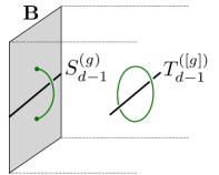
Figure 1: A Gukov-Witten operator $T_{d-1}^{([g])}$ in the bulk induces a prescribed holonomy along a small circle linking it. The holonomy is $g$ up to conjugation. The topological operator $S_{d-1}^{(g)}$ is “anchored” to $\mathbf{B}$. It induces a prescribed value $g$ for the quantity $\mathrm{Pexp}\int_{P}^{Q}a_{1}$ where $P$, $Q$ are the endpoints of a small semicircle linking $S_{d-1}^{(g)}$.

Crucially, in the bulk theory the Gauss’s law constraint holds and, because of gauge invariance, we can only write down topological operators labeled by conjugacy classes in the bulk gauge group, that are gauge invariant. On the contrary, gauge transformation asymptote to the identity at the boundary, and for this reason a global 0-form $G$ gauge symmetry is realized .

We can describe the topological operators $S^{(g)}_{d-1}$ on $\mathbf{B}$ as operators of $(d+1)$-dimensional $G$ Yang-Mills theory defined on a half-space. The support $M_{d-1}$ of $S^{(g)}_{d-1}$ is linked by a semicircle. Inserting $S^{(g)}_{d-1}$ means performing the path integral over $a_{1}$ on the half-space, with Dirichlet boundary conditions on the boundary $\mathbf{B}$, and imposing that the path-ordered exponential of the integral of $a_{1}$ along the semicircle equals $g$. See Figure 1. Crucially, this integral of $a_{1}$ on the semicircle is gauge invariant. This is because we can only perform gauge transformations in the half-space that are trivial at the boundary $\mathbf{B}$, and the endpoints of the semicircle lie on $\mathbf{B}$.

We emphasize that the topological operators $S^{(g)}_{d-1}$ are “anchored” to $\mathbf{B}$, and cannot be brought into the bulk of $\mathbf{S}$ (this would violate bulk gauge invariance, per the discussion above). We can, however, start with a Gukov-Witten operator $T_{d-1}^{([g])}$ in the bulk, and project it parallel onto the boundary $\mathbf{B}$. The resulting topological operator on $\mathbf{B}$ is not simple, but rather a sum of operators $S^{(g^{\prime})}_{d-1}$ with $g^{\prime}\in[g]$ . Only these averaged operators can move from the boundary into the bulk and viceversa.

Next, let us discuss charged local operators and how $G$ acts on them. Generalized charges have been studied extensively in recent works [83, 84, 85, 86, 23]. In the remainder of this section we follow closely the discussion in [83, 23]. For simplicity, we restrict to genuine local operators transforming in a representation $\mathbf{R}$. In the SymTFT picture these operators are engineered by stretching a Wilson line $W_{1}^{(\mathbf{R})}$ along the interval direction, connecting a point $\mathcal{M}$ on $\widehat{\mathbf{T}}$ to a point $\mathcal{E}$ on $\mathbf{B}$, see Figure 2. This configuration is allowed by our choice of Dirichlet boundary conditions for $a_{1}$ on $\mathbf{B}$.

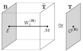
Figure 2: Sandwich construction for a genuine local operator $\mathcal{O}^{(\mathbf{R})}$ of the theory $\mathbf{T}$ in the representation $\mathbf{R}$ in terms of a Wilson line $W_{1}^{(\mathbf{R})}$ stretched between a topological endpoint $\mathcal{E}$ on $\mathbf{B}$ and a non-necessarily topological endpoint $\mathcal{M}$ on $\widehat{\mathbf{T}}$.

As stressed above, the topological operators $S_{d-1}^{(g)}$ labeled by elements of $G$ live on $\mathbf{B}$. Thus, the $G$-action is encoded on the action of $S_{d-1}^{(g)}$ on the endpoint $\mathcal{E}$ of $W_{1}^{(\mathbf{R})}$ on $\mathbf{B}$. This is to be contrasted, for instance, with the case of an Abelian global symmetry, for which the $G$-action can also be seen via linking in the bulk.

To describe more precisely the endpoint $\mathcal{E}$, we proceed as follows. We can consider the Wilson line $W_{1}^{(\mathbf{R})}$ and project it parallel onto the symmetry boundary $\mathbf{B}$. The result is

$$nS_{1}^{(\rm id)}:=\overbrace{S_{1}^{(\rm id)}\oplus\cdots\oplus S_{1}^{(\rm id)}}^{n\text{ times}}\ ,$$ (12)

where $S_{1}^{(\rm id)}$ is the identity topological line on $\mathbf{B}$ and $n$ is the dimension of the representation $\mathbf{R}$, see figure 3. (Indeed, due to Dirichlet boundary conditions, ${\rm Tr}_{\mathbf{R}}\mathrm{Pexp}\int a_{1}$ collapses to ${\rm Tr}_{\mathbf{R}}\mathbb{I}=\dim\mathbf{R}=n$.) Then, we can identify the possible endpoints $\mathcal{E}$ as the possible topological junctions $S_{0}$ between the lines $nS_{1}^{(\rm id)}$ and $S_{1}^{(\rm id)}$ in $\mathbf{B}$, see Figure 4. The vector space of such topological junctions is isomorphic to $\mathbb{C}^{n}$. This supports the identification of the possible endpoints $\mathcal{E}$ as the components of an operator transforming in the representation $\mathbf{R}$.

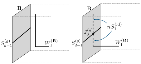
Figure 3: When the Wilson line $W_{1}^{(\mathbf{R})}$ is projected parallel to the boundary $\mathbf{B}$ it yields $nS_{1}^{(\mathrm{id})}$, denoted with a double dashed line. Projecting an L-shaped configuration for $W_{1}^{(\mathbf{R})}$ gives the canonical endpoint on $\mathbf{B}$ connecting $W_{1}^{(\mathbf{R})}$ and $nS_{1}^{(\mathrm{id})}$. When $W_{1}^{(\mathbf{R})}$ is projected on top of an operator $S_{d-1}^{(g)}$, we get the point-like topological junction $J_{0}^{(g)}$.

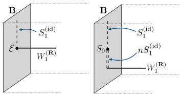
Figure 4: The endpoint $\mathcal{E}$ of $W_{1}^{(\mathbf{R})}$ is a junction with the trivial line $S_{1}^{\rm(id)}$ on $\mathbf{B}$. By projecting a segment of $W_{1}^{(\mathbf{R})}$ below $\mathcal{E}$, we resolve $\mathcal{E}$ as a topological junction $S_{0}$ between the lines $nS_{1}^{(\rm id)}$ and $S_{1}^{(\rm id)}$.

Let us now consider an insertion of a topological operator $S_{d-1}^{(g)}$ inside $\mathbf{B}$. When we project the bulk Wilson line $W_{1}^{(\mathbf{R})}$ parallel onto $\mathbf{B}$, we obtain a topological point-like junction $J_{0}^{(g)}$ between $S_{d-1}^{(g)}$ and the line $nS_{1}^{(\rm id)}$, see Figure 3. The vector space of such topological junctions is isomorphic to linear maps from $\mathbb{C}^{n}\rightarrow\mathbb{C}^{n}$, or $n\times n$ complex matrices. As shown in [23], these matrices do indeed form a representation of $G$. Finally, the action of $S_{d-1}^{(g)}$ on the endpoint $\mathcal{E}$ corresponds to fusing $J_{0}^{(g)}$ and $S_{0}$, to obtain a new $S_{0}^{\prime}$ junction between the lines $nS_{1}^{(\rm id)}$ and $S_{1}^{(\rm id)}$. Here $S_{0}$ and $S_{0}^{\prime}$ are identified with vectors in $\mathbb{C}^{n}$, $J_{0}^{(g)}$ with an $n\times n$ matrix, and the fusion implements the matrix multiplication $S_{0}^{\prime}=J_{0}^{(g)}S_{0}$. We have recovered the action of $g\in G$ on the components of the operator transforming in the representation $\mathbf{R}$.

A remark on gauging. In SymTFT for finite symmetries the gauging operation is obtained via a boundary-changing topological interface, exchanging Dirichlet with Neumann boundary conditions. There is a sharp difference in the case of the SymTFT for continuous non-Abelian symmetries. In the absence of ’t Hooft anomalies, the gauging operation consist of gauging the global symmetry $G^{(0)}$ along the boundary $\mathbf{B}$. This is the analogue of a Neumann boundary condition for a finite symmetry. Indeed, from this perspective, a ’t Hooft anomaly for $G^{(0)}$ is encoded in additional couplings in the bulk SymTFT which obstruct Neumann boundary conditions for the $G$ gauge field. The gauging process is non-topological and acts on the bulk-boundary system as a projector, that averages to zero all gauge non-invariant configurations. The resulting theory along the isomorphism in (1) is $\mathbf{T}$ coupled to a $d$-dimensional $G$ Yang-Mills sector by gauging its global $G$ symmetry.

V Conclusions and outlook

In this letter we have given a derivation in geometric engineering as well as in holography of the SymTFT for continuous non-Abelian zero-form symmetries. We find the latter is a $d+1$ dimensional Yang-Mills theory at zero coupling, whose flat subsector is dual to the non-Abelian BF theory with the same gauge group. For this reason our results can be seen as a derivation of the proposal in [31, 30]. However, the most convenient duality frame to study this system is provided by the gauge theory side, that can be used to address several key features of the SymTFT. A natural generalization of our findings indicates that for field theories in fewer dimensions, the relevant SymTFT can include topological limits of models that are not just gauge theories. This is the case of 4d SCFTs geometrically engineered in M-theory via conical singularities with $G(2)$-holonomy [70], see also [87].

Other natural questions that we leave open are in the context of the interplay of our SymTFT with the usual features of ordinary global symmetries, such as anomalies or spontaneous breaking. We plan to return on these topics in future work, thanks to another interesting duality, after ’t Hooft [88]. Namely one can view the $g_{\rm YM}=0$ limit as a $U(1)^{r}\rtimes\text{Weyl}(G)$ gauge theory, where $r$ and $\text{Weyl}(G)$ are the rank and Weyl group of $G$. This gives a very explicit way of characterizing the various operators at hand [37, 38]. In particular, one of the new features of topological defects as symmetries is that they have a higher structure (see e.g. [89] for a recent discussion). It would be interesting to explore the higher structure of non-Abelian continuous symmetries and its interplay with anomalies from the perspective advocated in this work.

As a final more speculative remark, our findings suggests a pathway to describe topological defects for spacetime symmetries as opposed to internal ones in terms of a gravitational $d+1$ bulk theory at zero coupling.

$|$

References

- Gaiotto et al. [2015] D. Gaiotto, A. Kapustin, N. Seiberg, and B. Willett, JHEP 02, 172 (2015), arXiv:1412.5148 [hep-th] .
- Cordova et al. [2022a] C. Cordova, T. T. Dumitrescu, K. Intriligator, and S.-H. Shao, in Snowmass 2021 (2022) arXiv:2205.09545 [hep-th] .
- McGreevy [2022] J. McGreevy, (2022), 10.1146/annurev-conmatphys-040721-021029, arXiv:2204.03045 [cond-mat.str-el] .
- Gomes [2023] P. R. S. Gomes, SciPost Phys. Lect. Notes 74, 1 (2023), arXiv:2303.01817 [hep-th] .
- Schafer-Nameki [2024] S. Schafer-Nameki, Phys. Rept. 1063, 1 (2024), arXiv:2305.18296 [hep-th] .
- Brennan and Hong [2023] T. D. Brennan and S. Hong, (2023), arXiv:2306.00912 [hep-ph] .
- Bhardwaj et al. [2024] L. Bhardwaj, L. E. Bottini, L. Fraser-Taliente, L. Gladden, D. S. W. Gould, A. Platschorre, and H. Tillim, Phys. Rept. 1051, 1 (2024), arXiv:2307.07547 [hep-th] .
- Shao [2023] S.-H. Shao, (2023), arXiv:2308.00747 [hep-th] .
- Carqueville et al. [2023] N. Carqueville, M. Del Zotto, and I. Runkel (2023) arXiv:2311.02449 [math-ph] .
- Ji and Wen [2020] W. Ji and X.-G. Wen, Phys. Rev. Res. 2, 033417 (2020), arXiv:1912.13492 [cond-mat.str-el] .
- Gaiotto and Kulp [2021] D. Gaiotto and J. Kulp, JHEP 02, 132 (2021), arXiv:2008.05960 [hep-th] .
- Apruzzi et al. [2023a] F. Apruzzi, F. Bonetti, I. n. García Etxebarria, S. S. Hosseini, and S. Schafer-Nameki, Commun. Math. Phys. 402, 895 (2023a), arXiv:2112.02092 [hep-th] .
- Freed et al. [2022] D. S. Freed, G. W. Moore, and C. Teleman, (2022), arXiv:2209.07471 [hep-th] .
- Gukov et al. [2021] S. Gukov, P.-S. Hsin, and D. Pei, JHEP 04, 232 (2021), arXiv:2010.15890 [hep-th] .
- Del Zotto and García Etxebarria [2023] M. Del Zotto and I. n. García Etxebarria, JHEP 11, 058 (2023), arXiv:2204.06495 [hep-th] .
- Bashmakov et al. [2023a] V. Bashmakov, M. Del Zotto, and A. Hasan, JHEP 09, 161 (2023a), arXiv:2206.07073 [hep-th] .
- Kaidi et al. [2023a] J. Kaidi, K. Ohmori, and Y. Zheng, Commun. Math. Phys. 404, 1021 (2023a), arXiv:2209.11062 [hep-th] .
- Bashmakov et al. [2023b] V. Bashmakov, M. Del Zotto, A. Hasan, and J. Kaidi, JHEP 05, 225 (2023b), arXiv:2211.05138 [hep-th] .
- Kaidi et al. [2023b] J. Kaidi, E. Nardoni, G. Zafrir, and Y. Zheng, JHEP 10, 053 (2023b), arXiv:2301.07112 [hep-th] .
- Chen et al. [2023] J. Chen, W. Cui, B. Haghighat, and Y.-N. Wang, JHEP 11, 208 (2023), arXiv:2305.09734 [hep-th] .
- Bashmakov et al. [2023c] V. Bashmakov, M. Del Zotto, and A. Hasan, (2023c), arXiv:2305.10422 [hep-th] .
- Antinucci et al. [2022a] A. Antinucci, C. Copetti, G. Galati, and G. Rizi, (2022a), arXiv:2212.09549 [hep-th] .
- Bhardwaj and Schafer-Nameki [2023a] L. Bhardwaj and S. Schafer-Nameki, (2023a), arXiv:2305.17159 [hep-th] .
- Sun and Zheng [2023] Z. Sun and Y. Zheng, (2023), arXiv:2307.14428 [hep-th] .
- Cordova et al. [2023] C. Cordova, P.-S. Hsin, and C. Zhang, (2023), arXiv:2308.11706 [hep-th] .
- Antinucci et al. [2023] A. Antinucci, F. Benini, C. Copetti, G. Galati, and G. Rizi, (2023), arXiv:2308.11707 [hep-th] .
- Bhardwaj et al. [2023a] L. Bhardwaj, L. E. Bottini, D. Pajer, and S. Schafer-Nameki, (2023a), arXiv:2310.03786 [cond-mat.str-el] .
- Bhardwaj et al. [2023b] L. Bhardwaj, L. E. Bottini, D. Pajer, and S. Schäfer-Nameki, (2023b), arXiv:2310.03784 [hep-th] .
- Bhardwaj et al. [2023c] L. Bhardwaj, L. E. Bottini, D. Pajer, and S. Schafer-Nameki, (2023c), arXiv:2312.17322 [hep-th] .
- Brennan and Sun [2024] T. D. Brennan and Z. Sun, (2024), arXiv:2401.06128 [hep-th] .
- Antinucci and Benini [2024] A. Antinucci and F. Benini, (2024), arXiv:2401.10165 [hep-th] .
- Note [1] Similar to the Abelian case discussed in [30, 31], our analysis applies to flat backgrounds of the continuous symmetry. These backgrounds are captured by the boundary conditions of our bulk TFT. We reserve a better treatment including more general backgrounds for future work.
- Horowitz [1989] G. T. Horowitz, Commun. Math. Phys. 125, 417 (1989).
- Note [2] We find it sacrilegious to form sandwiches out of quiches and therefore we refrain from using the terminology introduced in [13] in this note.
- [35] F. Apruzzi and F. Bedogna, to appear.
- Witten [1992] E. Witten, J. Geom. Phys. 9, 303 (1992), arXiv:hep-th/9204083 .
- Cordova et al. [2022b] C. Cordova, K. Ohmori, and T. Rudelius, JHEP 11, 154 (2022b), arXiv:2202.05866 [hep-th] .
- Antinucci et al. [2022b] A. Antinucci, G. Galati, and G. Rizi, JHEP 12, 061 (2022b), arXiv:2206.05646 [hep-th] .
- Note [3] Mutatis mutandis our results generalize straightfordwardly to type IIA geometric engineering limits, and little more effort is needed in the context of IIB or Heterotic scenarios, which we reserve to study in future work.
- Tian and Wang [2022] J. Tian and Y.-N. Wang, SciPost Phys. 12, 127 (2022), arXiv:2110.15129 [hep-th] .
- Del Zotto et al. [2022a] M. Del Zotto, J. J. Heckman, S. N. Meynet, R. Moscrop, and H. Y. Zhang, Phys. Rev. D 106, 046010 (2022a), arXiv:2201.08372 [hep-th] .
- van Beest et al. [2023] M. van Beest, D. S. W. Gould, S. Schafer-Nameki, and Y.-N. Wang, JHEP 02, 226 (2023), arXiv:2210.03703 [hep-th] .
- Apruzzi et al. [2023b] F. Apruzzi, I. Bah, F. Bonetti, and S. Schafer-Nameki, Phys. Rev. Lett. 130, 121601 (2023b), arXiv:2208.07373 [hep-th] .
- García Etxebarria [2022] I. n. García Etxebarria, Fortsch. Phys. 70, 2200154 (2022), arXiv:2208.07508 [hep-th] .
- Heckman et al. [2023a] J. J. Heckman, M. Hübner, E. Torres, and H. Y. Zhang, Fortsch. Phys. 71, 2200180 (2023a), arXiv:2209.03343 [hep-th] .
- Heckman et al. [2023b] J. J. Heckman, M. Hubner, E. Torres, X. Yu, and H. Y. Zhang, Phys. Rev. D 108, 046015 (2023b), arXiv:2212.09743 [hep-th] .
- Etheredge et al. [2023] M. Etheredge, I. Garcia Etxebarria, B. Heidenreich, and S. Rauch, JHEP 09, 005 (2023), arXiv:2302.14068 [hep-th] .
- Dierigl et al. [2024] M. Dierigl, J. J. Heckman, M. Montero, and E. Torres, Phys. Rev. D 109, 046004 (2024), arXiv:2305.05689 [hep-th] .
- Cvetič et al. [2024] M. Cvetič, J. J. Heckman, M. Hübner, and E. Torres, Phys. Rev. D 109, 046007 (2024), arXiv:2305.09665 [hep-th] .
- Bah et al. [2024] I. Bah, E. Leung, and T. Waddleton, JHEP 01, 117 (2024), arXiv:2306.15783 [hep-th] .
- Apruzzi et al. [2023c] F. Apruzzi, F. Bonetti, D. S. W. Gould, and S. Schafer-Nameki, (2023c), arXiv:2306.16405 [hep-th] .
- Baume et al. [2023] F. Baume, J. J. Heckman, M. Hübner, E. Torres, A. P. Turner, and X. Yu, (2023), arXiv:2310.12980 [hep-th] .
- Heckman et al. [2024a] J. J. Heckman, M. Hübner, and C. Murdia, (2024a), arXiv:2401.09538 [hep-th] .
- Heckman et al. [2024b] J. J. Heckman, J. McNamara, M. Montero, A. Sharon, C. Vafa, and I. Valenzuela, (2024b), arXiv:2402.00118 [hep-th] .
- [55] M. Del Zotto, S. N. Meynet, and R. Moscrop, In preparation.
- Del Zotto et al. [2016] M. Del Zotto, J. J. Heckman, D. S. Park, and T. Rudelius, Lett. Math. Phys. 106, 765 (2016), arXiv:1503.04806 [hep-th] .
- García Etxebarria et al. [2019] I. n. García Etxebarria, B. Heidenreich, and D. Regalado, JHEP 10, 169 (2019), arXiv:1908.08027 [hep-th] .
- Morrison et al. [2020] D. R. Morrison, S. Schafer-Nameki, and B. Willett, JHEP 09, 024 (2020), arXiv:2005.12296 [hep-th] .
- Albertini et al. [2020] F. Albertini, M. Del Zotto, I. n. García Etxebarria, and S. S. Hosseini, JHEP 12, 203 (2020), arXiv:2005.12831 [hep-th] .
- Hubner et al. [2022] M. Hubner, D. R. Morrison, S. Schafer-Nameki, and Y.-N. Wang, SciPost Phys. 13, 030 (2022), arXiv:2203.10022 [hep-th] .
- Benini et al. [2009] F. Benini, S. Benvenuti, and Y. Tachikawa, JHEP 09, 052 (2009), arXiv:0906.0359 [hep-th] .
- Del Zotto et al. [2015] M. Del Zotto, J. J. Heckman, A. Tomasiello, and C. Vafa, JHEP 02, 054 (2015), arXiv:1407.6359 [hep-th] .
- Hayashi et al. [2019] H. Hayashi, P. Jefferson, H.-C. Kim, K. Ohmori, and C. Vafa, (2019), arXiv:1905.00116 [hep-th] .
- Eckhard et al. [2020] J. Eckhard, S. Schäfer-Nameki, and Y.-N. Wang, JHEP 07, 199 (2020), arXiv:2004.15007 [hep-th] .
- Bhardwaj [2021a] L. Bhardwaj, JHEP 09, 186 (2021a), arXiv:2010.13230 [hep-th] .
- Bhardwaj [2021b] L. Bhardwaj, JHEP 04, 221 (2021b), arXiv:2010.13235 [hep-th] .
- Apruzzi et al. [2022] F. Apruzzi, S. Schafer-Nameki, L. Bhardwaj, and J. Oh, SciPost Phys. 13, 024 (2022), arXiv:2105.08724 [hep-th] .
- Del Zotto et al. [2022b] M. Del Zotto, J. Oh, and Y. Zhou, JHEP 08, 214 (2022b), arXiv:2109.01110 [hep-th] .
- Del Zotto et al. [2022c] M. Del Zotto, I. n. García Etxebarria, and S. Schafer-Nameki, SciPost Phys. 13, 105 (2022c), arXiv:2203.10097 [hep-th] .
- Acharya et al. [2023] B. S. Acharya, M. Del Zotto, J. J. Heckman, M. Hubner, and E. Torres, (2023), arXiv:2304.03300 [hep-th] .
- De Marco et al. [2023] M. De Marco, M. Del Zotto, M. Graffeo, and A. Sangiovanni, (2023), arXiv:2311.04984 [hep-th] .
- Note [4] In the case the holographic dictionary is slightly more complicated, as emphasized by Harlow and Ooguri [78]. In particular, for the analysis is subtler due to logarithmic scaling [90] and the possibility of quadratic Chern-Simons terms.
- Witten [1998a] E. Witten, Adv. Theor. Math. Phys. 2, 253 (1998a), arXiv:hep-th/9802150 .
- Note [5] See e.g. [91, 92, 93, 94, 43, 44, 46, 47, 50, 51, 53, 54], building on [95, 96].
- Berkooz [1998] M. Berkooz, Phys. Lett. B 437, 315 (1998), arXiv:hep-th/9802195 .
- Polchinski [2004] J. Polchinski, Int. J. Mod. Phys. A 19S1, 145 (2004), arXiv:hep-th/0304042 .
- Banks and Seiberg [2011] T. Banks and N. Seiberg, Phys. Rev. D 83, 084019 (2011), arXiv:1011.5120 [hep-th] .
- Harlow and Ooguri [2021] D. Harlow and H. Ooguri, Commun. Math. Phys. 383, 1669 (2021), arXiv:1810.05338 [hep-th] .
- Note [6] We are especially indebted to Kantaro Ohmori for a discussion that helped clarifying and shaping some key parts of this section, in particular, how the non-Abelian symmetry is realized along the boundary.
- Note [7] It would be interesting to investigate the connection between the Gukov-Witten operators we discuss in this note and the non-invertible averages introduced by Córdova, Ohmori and Rudelius in [37].
- Note [8] This is reminiscent of the construction of the Drinfeld Center of a symmetry category.
- Note [9] This would be an averaged operator over the Haar measure of the group, reminiscent of the discussion in [37].
- Lin et al. [2023] Y.-H. Lin, M. Okada, S. Seifnashri, and Y. Tachikawa, JHEP 03, 094 (2023), arXiv:2208.05495 [hep-th] .
- Bartsch et al. [2023a] T. Bartsch, M. Bullimore, and A. Grigoletto, (2023a), arXiv:2304.03789 [hep-th] .
- Bartsch et al. [2023b] T. Bartsch, M. Bullimore, and A. Grigoletto, (2023b), arXiv:2305.17165 [hep-th] .
- Bhardwaj and Schafer-Nameki [2023b] L. Bhardwaj and S. Schafer-Nameki, (2023b), arXiv:2304.02660 [hep-th] .
- Braun et al. [2023] A. P. Braun, E. Sabag, M. Sacchi, and S. Schafer-Nameki, (2023), arXiv:2304.01193 [hep-th] .
- ’t Hooft [1981] G. ’t Hooft, Nucl. Phys. B 190, 455 (1981).
- Copetti et al. [2023] C. Copetti, M. Del Zotto, K. Ohmori, and Y. Wang, (2023), arXiv:2305.18282 [hep-th] .
- Faulkner and Iqbal [2013] T. Faulkner and N. Iqbal, JHEP 07, 060 (2013), arXiv:1207.4208 [hep-th] .
- Bah et al. [2020] I. Bah, F. Bonetti, R. Minasian, and E. Nardoni, JHEP 01, 125 (2020), arXiv:1910.04166 [hep-th] .
- Bergman et al. [2020] O. Bergman, Y. Tachikawa, and G. Zafrir, JHEP 07, 077 (2020), arXiv:2004.05350 [hep-th] .
- Bah et al. [2021] I. Bah, F. Bonetti, and R. Minasian, JHEP 03, 196 (2021), arXiv:2007.15003 [hep-th] .
- Bergman and Hirano [2022] O. Bergman and S. Hirano, JHEP 11, 069 (2022), arXiv:2208.09396 [hep-th] .
- Witten [1998b] E. Witten, JHEP 12, 012 (1998b), arXiv:hep-th/9812012 .
- Belov and Moore [2004] D. Belov and G. W. Moore, (2004), arXiv:hep-th/0412167 .