Post-Minkowskian Theory Meets the Spinning Effective-One-Body Approach
for Two-Body Scattering

Abstract

Effective-one-body (EOB) waveforms employed by the LIGO-Virgo-KAGRA Collaboration have primarily been developed by resumming the post-Newtonian expansion of the relativistic two-body problem. Given the recent significant advancements in post-Minkowskian (PM) theory and gravitational self-force formalism, there is considerable interest in creating waveform models that integrate information from various perturbative methods in innovative ways. This becomes particularly crucial when tackling the accuracy challenge posed by upcoming ground-based detectors (such as the Einstein Telescope and Cosmic Explorer) and space-based detectors (such as LISA, TianQin or Taiji) expected to operate in the next decade. In this context, we present the derivation of the first spinning EOB Hamiltonian that incorporates PM results up to three-loop order: the SEOB-PM model. The model accounts for the complete hyperbolic motion, encompassing nonlocal-in-time tails. To evaluate its accuracy, we compare its predictions for the conservative scattering angle, augmented with dissipative contributions, against numerical-relativity data of non-spinning and spinning equal-mass black holes. We observe very good agreement, comparable, and in some cases slightly better to the recently proposed $w_{\rm EOB}$-potential model, of which the SEOB-PM model is a resummation around the probe limit. Indeed, in the probe limit, the SEOB-PM Hamiltonian and scattering angles reduce to the one of a test mass in Kerr spacetime. Once complemented with nonlocal-in-time contributions for bound orbits, the SEOB-PM Hamiltonian can be utilized to generate waveform models for spinning black holes on quasi-circular orbits.

I Introduction

The observation of gravitational waves (GWs) from coalescing binary black holes (BHs) and neutron stars (NSs) provides a unique opportunity to probe fundamental physics, dynamical gravity and matter under extreme conditions [1, 2, 3, 4, 5]. Having access to a large number of GW signals — more than 100 published observations by the LIGO-Virgo-KAGRA (LVK) Collaboration and independent analyses [6, 7, 8] at the time of writing — permits us to shed light on the astrophysical scenarios responsible for the formation of these binary systems [9]. Successful GW searches, precise inference of astrophysical and cosmological properties, and correct identifications of sources require detailed knowledge of the expected signals. This is achieved employing waveform models that are built by combining the best available methods to solve the two-body problem in General Relativity (GR).

On one side, for the inspiral stage of the binary coalescence, we can solve Einstein’s equations analytically, but approximately, in (i) the weak-field and small-velocity limit (i.e., in post-Newtonian (PN) theory [10, 11, 12, 13, 14]), (ii) in the weak-field regime (i.e., in post-Minkowskian (PM) theory [15, 16, 17, 18, 19, 20, 21, 22, 23, 24]), and (iii) in the small mass-ratio limit (i.e., in the gravitational-self force (GSF) formalism [25, 26, 27, 28, 29, 30, 31, 32, 33, 34, 35, 36, 37]). On the other side, for the late inspiral, merger and ringdown stages, we can solve the Einstein’s equations numerically [38, 39, 40] on supercomputers, obtaining highly accurate GW predictions. Performing simulations in numerical relativity (NR), however, is time consuming. Thus, NR cannot be used alone to build the several hundred thousands (millions) waveform models or templates that are used in matched-filtering searches (follow-up Bayesian analysis) [6]. Importantly, analytical and numerical results need to be combined synergistically to achieve the accuracy that is needed. This is obtained through the effective-one-body (EOB) formalism [41, 42, 43, 44, 45] that maps the two-body dynamics onto the dynamics of a test mass [43, 46, 47, 48, 49] (or test spin [50, 51, 52]) moving in a deformed Schwarzschild or Kerr spacetime, the deformation being the mass ratio. The EOB formalism also predicts the full coalescence waveform through physically motivated ansatze for the merger, and BH perturbation theory, and it can be made highly accurate through calibration to NR [53, 54, 55, 56, 57, 58, 59, 60, 61, 62, 63, 64, 65, 66, 67].

So far, EOB waveform models employed by the LVK Collaboration have been built on resummations of the PN expansion, except for Refs. [67, 68], which includes second-order GSF results [37] for the gravitational modes and radiation-reaction force. Given the recent results in PM [22, 23, 69, 70, 71, 72, 73, 74, 75, 76, 77, 78, 79, 80] and GSF [36, 37] theories, there is now great interest in exploring and developing waveform models that assemble the information from all the different perturbative methods, and in novel ways. This is particularly important when addressing the accuracy challenge posed by ever more sensitive detectors operating in the next decade: on the ground, such as the Einstein Telescope [81] and Cosmic Explorer [82], and in space, such as LISA [83], TianQin or Taiji, which demand an improvement of the waveforms by two orders of magnitude or more, depending on the parameter space [84, 85, 86], and the inclusion of all physical effects (spin-precession, eccentricity, matter). We remark that the LVK Collaboration also employs waveform models for the inspiral, merger and ringdown in frequency-domain by combining PN, EOB and NR results (i.e., the phenomenological templates [87, 88]), and waveforms that interpolate directly NR simulations (i.e., the NR-surrogate models [89, 90]).

Building on previous work [91, 92, 93, 94, 95, 49], in this paper we present the first EOB Hamiltonian for spinning bodies based on the PM expansion (henceforth, SEOB-PM) that includes complete non-spinning [76, 77, 96, 97, 98] and spinning information [99, 100, 101, 102, 103, 104, 105, 106, 107, 108, 109] through 4PM order for hyperbolic motion, with additional corrections at 5PM. Our PM counting is a physical one for compact objects, such as black holes and neutron stars, spin orders contributing as well as loop orders. We assess the accuracy of the SEOB-PM Hamiltonian by comparing its predictions for the scattering angle with available NR results [110, 111, 112] for nonspinning and spinning bodies with equal masses and equal spins. We contrast our model predictions with the non-spinning EOB model of Ref. [95], which is also based on an EOB Hamiltonian, and the $w_{\rm EOB}$-model, which was developed in Refs. [113, 112]. We also discuss its improvement against its PN counterpart and its comparison against the $w_{\rm EOB}$ model in the probe limit (and unequal-mass scatterings) since, differently from $w_{\rm EOB}$, the SEOB-PM model does reduce to the probe limit (i.e., it reduces to the Schwarzschild and Kerr results).

Importantly, the SEOB-PM model entails (or is based on) a Hamiltonian. Thus, it can be used to describe the two-body dynamics for bound orbits, and combined with a suitable radiation-reaction force and gravitational modes, it can be employed to generate waveform models for binary BHs with spins. To describe waveforms from quasi-circular orbits, Ref. [114] has augmented such a Hamiltonian with nonlocal-in-time terms at 4PN order [115, 116, 117, 118, 119] for bound orbits.

The paper is organized as follows. After summarizing the notation used in this work, in Sec. II we review the perturbative conservative and dissipative contributions to the scattering angle, and also estimate the effect of the recoil on the scattering angles of BHs carrying different spin magnitudes. In Sec. III, we highlight the scattering angle in the probe limit, i.e. for a test-mass in a hyperbolic orbit about the Kerr spacetime. In Sec. IV we derive the SEOB-PM Hamiltonian, resumming information at both 4PM and 5PM orders, which is the main result of this paper. In Sec. V we assess its validity by comparing its predictions for the scattering angle with NR data of Refs. [111, 112], and also with the so-called $w_{\rm EOB}$-potential model proposed in those papers. Finally, we summarize our main conclusions in Sec. VI.

Notation

Henceforth, we work in the (initial) center-of-mass (CoM) frame and employ natural units $G=c=1$. For our spinning two-body system, consisting of two scattered massive bodies (BHs), we introduce the following combinations of masses $m_{1}$, $m_{2}$:

$$M =m_{1}+m_{2}\,,\,\,\nu=\frac{\mu}{M}=\frac{m_{1}m_{2}}{M^{2}}\,,\,\,\delta=\frac{m_{1}-m_{2}}{M}\,,$$ (1)

so $\delta=\sqrt{1-4\nu}$ with $m_{1}\geq m_{2}$. We also introduce the total energy $E=E_{1}+E_{2}$ and effective energy $E_{\rm eff}$, which are related by the energy map:

$$\Gamma \equiv\frac{E}{M}=\sqrt{1+2\nu(\gamma-1)}\,,$$ (2a)

$$\gamma \equiv\frac{E_{\rm eff}}{\mu}=\frac{E^{2}-m_{1}^{2}-m_{2}^{2}}{2m_{1}m_{2}}\,.$$ (2b)

The boost factor $\gamma>1$ is given by

$$\gamma=\frac{1}{\sqrt{1-v^{2}}}\,,$$ (3)

where $v$ is the relativistic relative velocity.

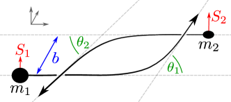
Figure 1: Kinematic setup of a planar two-body scattering event, with two separate scattering angles $\theta_{1}$, $\theta_{2}$ in the dissipative case. For the conservative dynamics, $\theta_{1}=\theta_{2}=\theta_{\rm cons}$. We specialize to aligned spins, with directed spin lengths $a_{1}=S_{1}/m_{1}$, $a_{2}=S_{2}/m_{2}$. (Diagram reproduced with minor edits from Ref. [120], with permission of the authors.)

The initial CoM frame, as defined with respect to the incoming momenta, is: $p_{1}^{\mu}=(E_{1},\bm{p}_{\infty}/\Gamma)$ and $p_{2}^{\mu}=(E_{2},-\bm{p}_{\infty}/\Gamma)$, where $p_{i}^{2}=m_{i}^{2}$ and $p_{1}\cdot p_{2}=\gamma\,m_{1}\,m_{2}$ — see Fig. 1. The relative CoM momentum at past infinity $\bm{p}_{\infty}$ has magnitude

$$p_{\infty}=|\bm{p}_{\infty}|=\mu\,v_{\infty}=\mu\sqrt{\gamma^{2}-1}\,.$$ (4)

The two bodies are initially separated by the impact parameter $\bm{b}$, with $\bm{b}\cdot\bm{p}_{\infty}=0$ and $b=|\bm{b}|$. As the motion evolves, we use the dynamical relative position and momentum vectors $\bm{r}$, $\bm{p}$ to describe the two-body motion:

$$\bm{p}^{2} =p_{r}^{2}+\frac{L^{2}}{r^{2}}\,, p_{r} =\hat{\bm{r}}\cdot\bm{p}\,, \bm{L}=\bm{r}\crossproduct\bm{p}\,,$$ (5)

where $r=|\bm{r}|$ and $\hat{\bm{r}}=\bm{r}/r$; $\bm{L}$ is the canonical orbital angular momentum with directed length $L=b\,p_{\infty}/\Gamma$. In the limit $r\to\infty$, we have $\bm{p}\to\bm{p}_{\infty}$. We also introduce $u=M/r$, which we use as the PM counting parameter, and $\ell=L/(M\mu)$ is the dimensionless orbital angular momentum.

Finally, we specialize to spin vectors $\bm{S}_{i}$ of the two bodies aligned with the orbital angular momentum $\bm{L}$. The total angular momentum $J$ is then given by

$$J =L+S_{1}+S_{2}\,, S_{i} =m_{i}a_{i}=m_{i}^{2}\chi_{i}\,.$$ (6)

Here $a_{i}$ are the directed spin lengths — for Kerr BHs, these are the radii of the ring singularities, and the dimensionless spin lengths are $-1<\chi_{i}<1$. Including, for clarity, units one has $S_{i}=Gm_{i}^{2}\chi_{i}/c$. We also introduce the combinations

$$a_{\pm} =M\chi_{\pm}=a_{1}\pm a_{2}\,.$$ (7)

Results from the PM-scattering literature are often given in terms of the covariant orbital angular momentum $L_{\rm cov}$. For aligned spins, the covariant orbital angular momentum $L_{\rm cov}$ is related to the total angular momentum $J$ by:

$$J =L_{\rm cov}+E_{1}a_{1}+E_{2}a_{2}\,.$$ (8)

Using Eq. (6) we may eliminate the total angular momentum $J$, and learn that

$$L_{\rm cov}=L-\frac{E-M}{2}\left(a_{+}-\frac{\delta}{\Gamma}a_{-}\right)\,.$$ (9)

We use this to re-express $L_{\rm cov}$ in terms of $L$.

II Perturbative Relativistic Scattering

Let us focus on two-body relativistic BH scattering events — depicted in Fig. 1. In order to prepare the ground for the scattering angles derived with the spinning EOB model based on PM (SEOB-PM) in Sec. IV, we focus first on the conservative and dissipative PM dynamics in Secs. II.1 and II.2, respectively, and then consider the probe motion in Sec. III. In connection with the PM regime, we also consider the PN and GSF expansions. Each of the three perturbative regimes may be defined by assuming certain combinations of the initial data to be small, of order $\epsilon\ll 1$. Using $M$ as a scale, the three dimensionless parameters, $1/\ell$, $v$ and $\nu$, together with the spins $S_{i}$, fully describe the initial state. The scalings of these parameters together with $u$ for the different perturbative schemes are summarized in Table 1. Notice that, in this physical counting scheme, the PM expansion does not align with the loop expansion, as it does in a formal counting — on dimensional grounds, powers of the spins $S_{i}=Gm_{i}^{2}\chi_{i}/c$ come with additional factors of $v$, $\ell$ and/or $u$, which are included in the counting. The scalings of other variables may be inferred by expressing them in terms of the basic ones in Table 1.

	$\ell^{-1}$	$v^{2}$	$\nu$	$u$
PM	$\sim\epsilon$	$\sim 1$	$\sim 1$	$\sim\epsilon$
PN	$\sim\sqrt{\epsilon}$	$\sim\epsilon$	$\sim 1$	$\sim\epsilon$
GSF	$\sim 1$	$\sim 1$	$\sim\epsilon$	$\sim 1$

Table 1: Scalings of the dimensionless variables $\ell$, $v$, $\nu$ and $u$ in the PM, PN and GSF regimes, with $\epsilon\ll 1$ a counting parameter. The dimensionless spins are taken with scaling $\chi_{i}\sim 1$ in all three regimes.

II.1 Conservative Scattering Angle

Let us first consider the ideal setting of conservative scattering, whose main characteristic is that the total energy and CoM angular momentum, $E$ and $L$, are conserved (implying in turn also that, e.g., $v$, $b$ and $p_{\infty}$ are conserved). In this case the motion is completely symmetric and fully described by the scattering angle which we label: $\theta_{\rm cons}$. This angle is related to the conservative momentum impulse $\Delta p^{\mu}_{\rm cons}=\Delta p^{\mu}_{1,\rm cons}=-\Delta p^{\mu}_{2,\rm cons}$ via

$$\sin\!\Big{(}\frac{\theta_{\rm cons}}{2}\Big{)}=\Gamma\,\frac{|\Delta p_{\rm cons}^{\mu}|}{2p_{\infty}}\ ,$$ (10)

which may be derived by geometrical arguments. In this setting the two angles $\theta_{i}$ of Fig. 1 are equal and denoted by $\theta_{\rm cons}$.

In this conservative approximation, the dynamics and scattering angle may equally well be described by a Hamiltonian. Rather than the Hamiltonian, in this section we find it useful to use the effective potential $w$ defined from the mass-shell constraint:

$$p_{r}^{2} =p_{\infty}^{2}-\frac{L^{2}}{r^{2}}+w(E_{\rm eff},L,r;a_{\pm})\,.$$ (11)

Using the Hamilton-Jacobi formalism (see e.g. Ref. [121]) the relationship between the potential and the angle is:

$$\theta+\pi=-2\int_{r_{\rm min}}^{\infty}\!{\rm d}r\frac{\partial}{\partial L}p_{r}\,,$$ (12)

where $r_{\rm min}$ is the closest point of approach defined as the largest root of $p_{r}(r_{\rm min})=0$. Here, we have omitted the ‘cons’ subscript on the angle, because in Sec. II.2 we also define a “dissipative” effective potential. This formula is generic, and applies both to the conservative setting discussed here and the dissipative effects to be discussed in Sec. II.2.

By way of Eq. (12), the scattering angle $\theta$ and the effective potential $w$ are in one-to-one correspondence. An expression for the potential in isotropic gauge in terms of the angle is given by the Firsov formula discussed in Refs. [70, 113]. While the angle is gauge-invariant, the potential is not; thus, it is uniquely determined by the angle only when a gauge condition is imposed. Nevertheless, the potential has certain advantages over the angle: it is finite in the PN limit and it has a simple expression (compared with the angle, see e.g. Ref [122]) in the probe limit. The angle generally depends on the dimensionless initial state variables ($\gamma$, $\nu$, $\ell$ and $\chi_{i}$), while the potential, in addition to these, also depends on the relative position, $u$ (and on $M$ to balance dimensions).

The PM expansions of the angle and potential are:

$$\theta =\sum_{n\geq 1}\frac{\theta^{(n)}}{\ell^{n}}\,,$$ (13a)

$$w =\sum_{n\geq 1}u^{n}w^{(n)}\,,$$ (13b)

$n$ counting the PM orders with PM expansion variables $1/\ell$ and $u$ (see Table 1). We define also $m$PM accurate scattering angles: $\theta^{m{\rm PM}}=\sum_{n=1}^{m}\theta^{{(n)}}/\ell^{n}$. We may further expand the PM coefficients with respect to the BHs’ spins:

$$\theta^{(n)} =\sum_{s=0}^{n-1}\sum_{i=0}^{s}\theta^{(n)}_{(s-i,i)}\delta^{\sigma(i)}\chi_{+}^{s-i}\chi_{-}^{i},$$ (14a)

$$w^{(n)} =\sum_{s=0}^{n}(\ell u)^{\sigma(s)}\sum_{i=0}^{s}w^{(n)}_{(s-i,i)}\delta^{\sigma(i)}\chi_{+}^{s-i}\chi_{-}^{i}.$$ (14b)

Here, $s$ counts the spin orders and $i$ the powers of $\chi_{-}$. The function $\sigma$ is given as

$$\sigma(n)=\begin{cases}0\,,&n\text{ even},\\ 1\,,&n\text{ odd},\end{cases}$$ (15)

and controls the introduction of $\delta$ to terms with odd powers of $\chi_{-}$ and a power of $\ell\,u$ for odd $s$ in the potential.

	$S^{0}$	$S^{1}$	$S^{2}$	$S^{3}$	$S^{4}$	$S^{5}$
tree level	1PM	2PM	3PM	4PM	5PM	6PM
1-loop	2PM	3PM	4PM	5PM	6PM	7PM
2-loop	3PM	4PM	5PM	6PM	7PM	8PM
3-loop	4PM	5PM	6PM	7PM	8PM	9PM
4-loop	5PM	6PM	7PM	8PM	9PM	10PM

Table 2: The relation between loop orders, spin orders and physical PM orders (as adopted in this work), with currently known results for the aligned-spin scattering angle $\theta$ colored in. The tree-level all-order-spin angle is given in Eq. (34). The 1-loop angle is known up to quartic $G^{6}$ order in spin [103, 104], with higher-order predictions in Refs. [123, 124, 125]. The 2-loop $G^{3}$ conservative dynamics were derived in Refs. [23, 126, 127, 128, 71], extended to include radiation [129, 130, 131, 132, 133, 134, 135, 136, 137] and $G^{4}$, $G^{5}$ linear- and quadratic-in-spin effects [105, 106, 107]. The 3-loop non-spinning $G^{4}$ terms were obtained in Refs. [76, 77] (conservative) and [96, 97, 98] (full dissipative). Spin-orbit effects ($G^{5}$) were incorporated in Refs. [108, 109].

$\theta$	0PN	1PN	2PN	3PN	4PN
1PM $S^{0}$	${\ell^{-1}v^{-1}}^{\vphantom{L}}$	${\ell^{-1}v}^{\vphantom{L}}$	${\ell^{-1}v^{3}}^{\vphantom{L}}$	${\ell^{-1}v^{5}}^{\vphantom{L}}$	${\ell^{-1}v^{7}}^{\vphantom{L}}$
2PM $S^{0}$		${\ell^{-2}}^{\vphantom{L}}$	${\ell^{-2}v^{2}}^{\vphantom{L}}$	${\ell^{-2}v^{4}}^{\vphantom{L}}$	${\ell^{-2}v^{6}}^{\vphantom{L}}$
3PM $S^{0}$	${\ell^{-3}v^{-3}}^{\vphantom{L}}$	${\ell^{-3}v^{-1}}^{\vphantom{L}}$	${\ell^{-3}v}^{\vphantom{L}}$	${\ell^{-3}v^{3}}^{\vphantom{L}}$	${\ell^{-3}v^{5}}^{\vphantom{L}}$
4PM $S^{0}$			${\ell^{-4}}^{\vphantom{L}}$	${\ell^{-4}v^{2}}^{\vphantom{L}}$	${\ell^{-4}v^{4}(*)}^{\vphantom{L}}$
5PM $S^{0}$	$\ell^{-5}v^{-5}$	$\ell^{-5}v^{-3}$	${\ell^{-5}v^{-1}}$	${\ell^{-5}v}$	${\ell^{-5}v^{3}(*)}$
3PM $S^{2}$			${\ell^{-3}v}^{\vphantom{L}}$	${\ell^{-3}v^{3}}^{\vphantom{L}}$	${\ell^{-3}v^{5}}^{\vphantom{L}}$
4PM $S^{2}$			${\ell^{-4}}^{\vphantom{L}}$	${\ell^{-4}v^{2}}^{\vphantom{L}}$	${\ell^{-4}v^{4}}^{\vphantom{L}}$
5PM $S^{2}$			$\ell^{-5}v^{-\!1}$	${\ell^{-5}v}^{\vphantom{L}}$	${\ell^{-5}v^{3}}^{\vphantom{L}}$
5PM $S^{4}$					$\ell^{-5}v^{3}$
$\theta$	0.5PN	1.5PN	2.5PN	3.5PN	4.5PN
2PM $S^{1}$		${\ell^{-2}v}^{\vphantom{L}}$	${\ell^{-2}v^{3}}^{\vphantom{L}}$	${\ell^{-2}v^{5}}^{\vphantom{L}}$	${\ell^{-2}v^{7}}^{\vphantom{L}}$
3PM $S^{1}$		${\ell^{-3}}^{\vphantom{L}}$	${\ell^{-3}v^{2}}^{\vphantom{L}}$	${\ell^{-3}v^{4}}^{\vphantom{L}}$	${\ell^{-3}v^{6}}^{\vphantom{L}}$
4PM $S^{1}$		${\ell^{-4}v^{-1}}^{\vphantom{L}}$	${\ell^{-4}v}^{\vphantom{L}}$	${\ell^{-4}v^{3}}^{\vphantom{L}}$	${\ell^{-4}v^{5}}^{\vphantom{L}}$
5PM $S^{1}$			${\ell^{-5}}^{\vphantom{L}}$	${\ell^{-5}v^{2}}^{\vphantom{L}}$	${\ell^{-5}v^{4}}^{\vphantom{L}}$
4PM $S^{3}$				${\ell^{-4}v^{3}}^{\vphantom{L}}$	${\ell^{-4}v^{5}}^{\vphantom{L}}$
5PM $S^{3}$				${\ell^{-5}v^{2}}^{\vphantom{L}}$	${\ell^{-5}v^{4}}^{\vphantom{L}}$

(a)

$w$	0PN	1PN	2PN	3PN	4PN
1PM $S^{0}$	${u}^{\vphantom{L}}$	${u\,v^{2}}^{\vphantom{L}}$	${u\,v^{4}}^{\vphantom{L}}$	${u\,v^{6}}^{\vphantom{L}}$	$u\,v^{8}$
2PM $S^{0}$		${u^{2}}^{\vphantom{L}}$	${u^{2}v^{2}}^{\vphantom{L}}$	${u^{2}v^{4}}^{\vphantom{L}}$	$u^{2}v^{6}$
3PM $S^{0}$			${u^{3}}^{\vphantom{L}}$	${u^{3}v^{2}}^{\vphantom{L}}$	$u^{3}v^{4}$
4PM $S^{0}$				${u^{4}}^{\vphantom{L}}$	$u^{4}v^{2}(*)$
5PM $S^{0}$					$u^{5}(*)$
3PM $S^{2}$			$u^{3}$	$u^{3}v^{2}$	$u^{3}v^{4}$
4PM $S^{2}$				$u^{4}$	$u^{4}v^{2}$
5PM $S^{2}$					$u^{5}$
5PM $S^{4}$					$u^{5}$
$w$	0.5PN	1.5PN	2.5PN	3.5PN	4.5PN
2PM $S^{1}$		$\ell u^{3}$	$\ell u^{3}v^{2}$	$\ell u^{3}v^{4}$	$\ell u^{3}v^{6}$
3PM $S^{1}$			$\ell u^{4}$	$\ell u^{4}v^{2}$	$\ell u^{4}v^{4}$
4PM $S^{1}$				$\ell u^{5}$	$\ell u^{5}v^{2}$
5PM $S^{1}$					$\ell u^{6}$
4PM $S^{3}$				$\ell u^{5}$	$\ell u^{5}v^{2}$
5PM $S^{3}$					$\ell u^{6}$

(b)

Table 3: Schematic overview of the terms appearing in a combined PM and PN expansion of the angle (left) and potential (right). In these expansions, terms with the above scalings in $\ell$, $v$ and $u$ appear with coefficients depending only on the symmetric mass ratio $\nu$ and the dimensionless spins $\chi_{\pm}$ (neither of which scales in the PM or PN expansions); empty cells are absent from the expansion. The explicitly shown terms are valid for the conservative dynamics, while the green shaded cells also pick up a 0.5PN subleading dissipative correction. The cells marked with a $(*)$ also have a tail contribution, implying $\log(v)$-dependence. The PN counting of the potential $w$ matches that of the Hamiltonian — see, e.g., Ref. [138]. The analytic results of all PM rows (to all PN orders) are known except for 5PM $S^{0}$ — see Table 2. The green shading and tail terms of the 5PM $S^{0}$ row are thus only an expectation.

As seen from Eq. (14a), the $n$PM angle gets contributions only from spin orders $s<n$. Our physical PM counting, valid for compact objects, is different from the formal PM counting often used in the PM literature, which aligns with the loop order. The relation between the physical PM counting relevant for spinning BHs and the formal loop-order PM counting is summarized in Table 2. Essentially, an $l$-loop result at spin order $s$ contributes to the $(l+s+1)$-PM order, so that both loops and spin orders climb up in PM orders. Colored entries of Table 2 indicate known results. The expansion coefficients of the angle depend non-trivially only on $\gamma$ and, when suitable variables are chosen and up to overall factors, on polynomials of the mass ratio (i.e., the mass polynomiality first observed in Refs. [99, 139]).

The PM expansion of the potential $w$ takes a particularly simple form in quasi-isotropic gauge, which is defined by requiring that the expansion coefficients of Eq. (14b) $w_{(j,i)}^{(n)}$ depend only on $\gamma$ and the masses, and that the sum on $s$ terminates at $n-1$ (i.e. $w^{(n)}_{(n-i,i)}=0$ for all $i$). We refer to this potential generally as $w_{{\rm PM}}$; or, up to a specified PM order, $w_{n{\rm PM}}$:

$$w_{n{\rm PM}}=\sum_{m=1}^{n}\sum_{s=0}^{m-1}\ell^{\sigma(s)}\sum_{i=0}^{s}w_{{\rm PM},(s-i,i)}^{(m)}\delta^{\sigma(i)}\chi_{+}^{s-i}\chi_{-}^{i}\,.$$ (16)

In Refs. [113, 112] it was shown that this potential defines a useful resummation of the angle: simply by inserting $w_{n\text{PM}}$ into Eq. (12), one already finds a good agreement with the NR scattering angles (in particular, when incorporating dissipative effects as discussed in Sec. II.2). In the same two papers, this computation of the scattering angles was dubbed $w_{\rm EOB}$. In the present work, however, we prefer to refer to a model as an EOB model only if it reproduces the probe motion in the limit $\nu\to 0$. That is, from a PM perspective, we require that the EOB model incorporates all PM orders in the $\nu\to 0$ limit, which is not the case for $w_{n\text{PM}}$. The computation of the PM-expanded scattering angle through Eq. (16) also coincides with Refs. [70, 140], where it was dubbed “$f_{n}$-theory” (for non-spinning 2PM dynamics).

The PM expansion of the potential $w$ in the SEOB-PM model (see Sec. IV) takes a more general form with dependence of $w_{(j,i)}^{(n)}$ on $\ell u$ and non-zero $w_{(n-i,i)}^{(n)}$. Note, however, that the SEOB-PM $\nu$-deformation parameters, have the same simplicity as the $w_{\text{PM}}$ expansion coefficients.

Let us finally analyze the PN structure of the scattering angle and $w_{\rm PM}$ potential, which is schematically shown in Table 3. The PM/PN structure of $w_{\rm PM}$ is identical to the PM/PN structure of the SEOB-PM deformations to be introduced below — except for the 1PM correction which is absent for SEOB-PM. Thus, we refer to it generically in Table 3 as $w$. In Table 3, all scalings of $v$, $\ell$ and $u$ are shown in a combined PM and PN expansion up to 5PM and 4.5PN, respectively. This table illustrates a key advantage of the potential over the angle, namely that in the angle, 0PN terms appear with arbitrarily high PM orders. Instead, for the potential 0PN is completely determined by 1PM and generally, $n$PN is completely determined by $(n+1)$PM. Table 3 also illustrates how spin pushes results to both higher PM and PN orders. The green shaded cells indicate terms that receive a dissipative correction at a subleading 0.5PN order, which we discuss in the next section. As stated above, full analytic PM results exist for all rows of Table 3 except the spinless row at 5PM. For the non-spinning, conservative PN angle, PN resummations along the columns to 3PN order can be found in Ref. [141] (including, also, partial 4PN order results).

To illustrate these points, the 1PM row and 0PN columns are, respectively, given by the following two expressions:

$$\theta =\frac{2}{\ell v}\frac{1+v^{2}}{\sqrt{1-v^{2}}}+\mathcal{O}\bigg{(}\frac{1}{\ell^{2}}\bigg{)}$$ (17a)

$$=2\text{arctan}\bigg{(}\frac{1}{\ell v}\bigg{)}+\mathcal{O}(v^{2})\ .$$ (17b)

The expansion of the second line in $1/\ell$ clearly illustrates that the 0PN angle gets contributions at arbitrarily high (odd) PM orders. Yet both of these limits are included in the $w_{\rm 1PM}$ angle:

$$\theta^{w}_{\rm 1PM} =2\text{arctan}\Bigg{(}\frac{1}{\ell v}\frac{1+v^{2}}{\sqrt{1-v^{2}}}\Bigg{)}\,,$$ (18)

which clearly reproduces Eqs. (17a) and (17b) in their respective limits. This angle agrees with expressions found in Refs. [70, 113].

II.2 Dissipative Effects

Naturally, the true relativistic two-body system is dissipative. As seen from the initial CoM frame, each BH loses energy, and so the two momentum impulses $\Delta p_{i}^{\mu}$ generally differ:

$$\Delta p_{1}^{\mu}+\Delta p_{2}^{\mu}=\Delta P^{\mu}\neq 0\ .$$ (19)

The four vector $\Delta P^{\mu}$ describes the total loss of linear momentum of the system. If this vector has a non-zero spatial part with respect to the initial CoM frame, then the final CoM frame (defined from $p_{i}^{\mu}+\Delta p_{i}^{\mu}$) is different from the initial one. This effect is referred to as recoil, and we define the spatial part of $\Delta P^{\mu}=(\Delta E,\Delta\bm{P})$ with respect to the initial CoM frame as the recoil vector.

A non-zero recoil implies, and is implied by, unequal scattering angles of the two bodies — see Fig. 1. In this more general setting, the scattering of either body is computed by the geometric formula,

$$\cos\theta_{i}=\frac{(\bm{p}_{i}+\Delta\bm{p_{i}})\cdot\bm{p}_{i}}{|\bm{p}_{i}+\Delta\bm{p_{i}}||\bm{p}_{i}|}\ .$$ (20)

With zero recoil, $\Delta\bm{p}_{1}=-\Delta\bm{p}_{2}$, and the two angles are equal (using, also, $\bm{p}_{1}=-\bm{p}_{2}$). At leading order in the PM expansion, one finds for the angle difference $\theta_{1}-\theta_{2}$ that

$$\theta_{1}-\theta_{2}=\frac{\Gamma}{p_{\infty}}\bigg{(}\frac{\bm{\Delta P}\cdot\bm{b}}{b}-\frac{\bm{\Delta P}\cdot\bm{p}_{\infty}}{p_{\infty}}\theta_{\rm cons}\bigg{)}+.\,.\,.$$ (21)

For generic masses, this effect starts at 4PM order because the recoil starts at 3PM in the $\bm{p}_{\infty}$ direction and at 4PM in the $\bm{b}$ direction (the leading-order 1PM part of $\theta_{\rm cons}$ balances the counting).

In the comparisons with NR in this work, we only consider equal-mass scattering scenarios. In this case, the recoil $\bm{\Delta P}$ is proportional to $\chi_{-}$ and therefore suppressed by one further PM order (so that $\theta_{1}-\theta_{2}$ starts at 5PM order). This is because, generally, the recoil is a symmetric function of the two black holes: its coefficients of $\bm{b}$ and $\bm{p_{\infty}}$ must be antisymmetric, and therefore include either $\delta$ or $\chi_{-}$. For the kinematics relevant to the NR comparisons of this work, namely $\nu=1/4$, $\Gamma=1.023$ and $\ell=4.58$, Eq. (21) evaluates to:

$$\theta_{1}^{\rm 5PM}-\theta_{2}^{\rm 5PM}\approx-8.4^{\circ}\times 10^{-4}\chi_{-}\ .$$ (22)

Hence, this effect is extremely small compared, e.g., to the 4PM scattering angle, which for these kinematics (and to leading order in spins) takes the value $\theta^{\rm 4PM}\approx 144.5^{\circ}+\mathcal{O}(\chi_{\pm})$. We mostly therefore ignore this effect in our subsequent comparisons of the angle with NR data. We note also that the 5PM effect in Eq. (22) is an order of magnitude smaller than the 4PM effect due to unequal masses, which at its maximum for $\nu\approx 0.17$ (and, as before, $\Gamma=1.023$ and $\ell=4.58$) takes the value $\theta^{\rm 4PM}_{1}-\theta^{\rm 4PM}_{2}\approx\pm 5.1^{\circ}\times 10^{-3}$ with a minus (plus) sign for $m_{1}>m_{2}$ ($m_{2}<m_{1}$).

With the presence of recoil, one may still define a relative scattering angle which is symmetric in the two BHs. One possibility involves the covariant impulse $\Delta p_{\rm rel}^{\mu}$ of the relative momentum:

$$p^{\mu}_{\rm rel}=(0,\bm{p}_{\infty})=\frac{E_{2}p_{1}^{\mu}-E_{1}p_{2}^{\mu}}{M}\ .$$ (23)

This impulse is defined by considering the change of each variable of the right-most side of Eq. (23) including the energies $E_{i}$. The relative scattering angle $\theta_{\rm rel}$ is then defined by:

$$\cos\theta_{\rm rel}=\frac{(\bm{p}_{\infty}+\Delta\bm{p_{\rm rel}})\cdot\bm{p}_{\infty}}{|\bm{p}_{\infty}+\Delta\bm{p_{\rm rel}}|p_{\infty}}\ .$$ (24)

This angle was first computed at 4PM order in Ref. [96] (from where we have adopted the relative subscript), and the 5PM spin-orbit part in Ref. [109]. This relative scattering angle is defined for dissipative motion including recoil.

In the following comparisons against NR (Sec. V), we will work with equal masses and spins in which case the recoil vanishes. Generally, for a vanishing recoil the relative scattering angle of Eq. (24) coincides with the (also coinciding) individual angles $\theta_{i}$. Dissipative effects, however, may still be non-zero. More generally, for a non-zero recoil, we are not aware of any simple relationship between the relative angle and the individual angles.

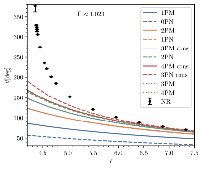
(a)

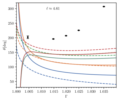
(b)

Figure 2: The perturbative scattering angle $\theta$ plotted at different PM and PN orders, conservative “cons” or full dissipative, compared with NR-data points [111, 112]. Both plots have equal masses and zero spins, absence of recoil at these perturbative orders thus implying $\theta_{\rm rel}=\theta_{1}=\theta_{2}$. To the left, we fix energy while varying angular momentum; to the right vice versa. As pointed out in Ref. [113] for the PM case, the perturbative angles do not perform well when the NR scattering angles become too large (close to the critical angular momentum). These results change drastically, and approach the NR data, when evaluating the scattering angle (12) without first expanding it perturbatively (in PM or PN), thus capturing the pole at the critical angular momentum.

We define a split of the relative angle into conservative and dissipative effects by writing:

$$\theta_{\rm rel}=\theta_{\rm cons}+\theta_{\rm diss}\ .$$ (25)

Since the conservative and relative angles have been defined above in Eqs. (10) and (24), the present equation defines the remaining part $\theta_{\rm diss}$ (naturally, when dissipation is negligible, this equation is an identity because then $\theta_{\rm rel}$ and $\theta_{\rm cons}$ coincides). Similarly to the conservative angle we may determine an effective potential $w_{\rm rel}$ that, when using Eqs. (11) and (12), reproduces $\theta_{\rm rel}$. While the physical intutition for this potential is less clear, one can certainly always imagine a conservative system that reproduces a given scattering angle. This idea was pursued in Refs. [113, 112], where it was seen to improve the $w_{\rm PM}$ model drastically (this idea was also suggested in Ref. [144]).

In the PM expansion of the scattering angles, dissipative effects first appear at the 3PM order (without, yet, any recoil effects). Generally, until the 4PM order, one may distinguish between odd and even dissipative effects. In the scattering angle, they come at half-integer or integer PN orders respectively for even order in spins and for odd orders, it is reversed (the same pattern is true for the potential). From the PM loop integration perspective, they appear from one or two radiative (on-shell) gravitons respectively [97, 109]. Dissipation at 3PM is only odd while even dissipation starts at 4PM. Until 4PM order it was shown that the odd part can be reconstructed from the conservative angle through linear response [145, 109]. For similar kinematics as considered above, namely $\nu=1/4$, $\Gamma=1.023$ and $\chi_{\pm}=0$, one finds that the odd dissipative effects are much larger than the even:

$$\frac{\theta^{\rm 4PM}_{\rm odd\,diss}}{\theta^{\rm 4PM}_{\rm even\,diss}}\approx 32.2\,\ell+578.3\ .$$ (26)

Because of the equal masses, there is no ambiguity of the angle here (i.e., $\theta_{1}=\theta_{2}=\theta_{\rm rel}$).

Let us discuss the appearance of dissipative effects in the combined PM and PN expansion of the relative angle. As already mentioned, dissipative effects start at non-spinning 3PM, and each of the spins push that to one higher PM order (i.e., dissipative effects start uniformly at 2-loop order, see Table 2). In the PN expansion, odd dissipation starts at spinless 2.5PN order and, again, spin pushes this to higher PN orders. In Table 3, dissipative terms are indicated by green shaded cells. All dissipative corrections up to 4PN that are shown there are odd. Instead, even dissipative effects in the 4PM scattering angle first appear at 5PN. Again, all dissipative PM results are known except for the spinless 5PM angle. We are, however, not aware of a dissipative result for the PN angle in the sense of Eq. (17b), which would resum the 2.5PN spinless column of Table 3. We note that the dissipative effects of the potential as defined in the present work do not seem to have the same upper triangular pattern as the conservative results. As the 5PM $S^{0}$ terms are not yet known, however, we cannot draw any definite conclusions.

Let us finally consider how the perturbative $n$PM and $m$PN scattering angles compare against equal-mass, nonspinning NR data. In Fig. 2 we plot these angles for $1\leq n\leq 4$ and $0\leq m\leq 3$ against NR data from Refs. [111, 112] (the PM curves of the left panel have already appeared in Refs. [95, 113]). For $n\geq 3$ and $m\geq 3$ we distinguish between the conservative angles (labelled cons) and the dissipative ones (where, again, equal mass means that $\theta_{1}=\theta_{2}=\theta_{\rm rel}$). Clearly, in the left panel, both the higher-order perturbative PM and PN angles describe the NR data well for sufficiently large angular momentum $\ell$. Generally, however, as noticed in Ref. [113], close to the critical angular momentum beyond which the plunge occurs, the agreement between the perturbative angles and NR is poor. This is due to the fact that by expanding Eq. (12) (with $p_{r}$ from Eq. (11)) perturbatively (PN or PM), one cannot capture the pole in the scattering angle corresponding to the critical angular momentum.

Furthermore, in the right panel of Fig. 2, where the energy is varied, one notes a clear difference between the PN and PM angles. In the low velocity $v\to 0$ limit ($\Gamma\to 1$), the PN angles have a finite limit while the PM angles diverge. One can easily read off the $v\to 0$ asymptotic behavior with fixed $\ell$ of the $n$PM angles from the (spinless) 0PN column of Table 3:

$$\theta^{2n{\rm PM}}\sim\theta^{(2n+1){\rm PM}}\sim v^{-2n-1}\ .$$ (27)

However, after resumming the entire column one finds the result in Eq. (17b), namely $2\text{arctan}(1/\ell v)$, with the finite limit $\pi$ ($180^{\circ}$).

For the phase space points considered in Fig. 2, dissipative effects of the PM angle are very small. However, when computing the results by evaluating the scattering angle from Eq. (12) without first expanding it perturbatively (in PM or PN), thus capturing the pole at the critical angular momentum, this is no longer the case, as found in the PM case in Ref. [113]. We note that Eq. (26) which compares odd and even dissipation is valid for the phase space points of the left panel. We may therefore gather that, for this kinematics, the conservative part is much larger than the odd dissipation which is much larger than the even dissipation: $\theta^{\rm 4PM}_{\rm cons}\gg\theta_{\rm odd\,diss}^{\rm 4PM}\gg\theta_{\rm even\,diss}^{\rm 4PM}$.

III Scattering in the Probe Limit

To prepare for our discussion of the SEOB-PM model, let us also review the simple case of a non-spinning probe of mass $\mu$, moving under the influence of a Kerr BH. In Boyer-Lindquist coordinates $(t,r,\theta,\phi)$, where $p_{\mu}=(E_{\rm Kerr},-p_{r},-p_{\theta},-p_{\phi})$, the (inverse) Kerr metric takes the form (see, e.g.,  Ref. [52])

$$\begin{aligned} g^{\mu\nu}_{\rm Kerr}\partial_{\mu}\partial_{\nu}&=\frac{\Lambda}{\Delta\Sigma}\partial_{t}^{2}-\frac{\Delta}{\Sigma}\partial_{r}^{2}-\frac{1}{\Sigma}\partial_{\theta}^{2}\\ &\qquad-\frac{\Sigma-2Mr}{\Sigma\Delta\sin^{2}\theta}\partial_{\phi}^{2}+\frac{4Mra}{\Sigma\Delta}\partial_{t}\partial_{\phi}\,,\end{aligned}$$ (28)

where we have introduced

$$\Sigma =r^{2}+a^{2}\cos^{2}\theta\,,$$ (29a)

$$\Delta =r^{2}-2Mr+a^{2}\,,$$ (29b)

$$\Lambda =(r^{2}+a^{2})^{2}-a^{2}\Delta\sin^{2}\theta\,.$$ (29c)

Specializing to aligned spins, we restrict ourselves to the orbital plane $\theta={\textstyle\frac{\pi}{2}}$. We find it helpful to introduce the specific combinations (as done in Ref. [49]):

$$A^{\rm Kerr} =\frac{\Delta\Sigma}{\Lambda}=\frac{1-2u+\chi^{2}u^{2}}{1+\chi^{2}u^{2}(2u+1)}\,,$$ (30a)

$$B_{\rm np}^{\rm Kerr} =\frac{r^{2}}{\Sigma}\left(\frac{\Delta}{r^{2}}-1\right)=\chi^{2}u^{2}-2u\,,$$ (30b)

$$B_{\rm npa}^{\rm Kerr} =-\frac{r^{2}}{\Sigma\Lambda}\left(\Sigma+2Mr\right)=-\frac{1+2u}{r^{2}+a^{2}(1+2u)}\,,$$ (30c)

where $a=m\chi$. We can now solve the mass-shell constraint $g^{\mu\nu}_{\rm Kerr}p_{\mu}p_{\nu}=\mu^{2}$ for the radial momentum $p_{r}$:

$$p_{r}^{2} =\frac{1}{(1+B_{\rm np}^{\rm Kerr})}\bigg{[}\frac{1}{A^{\rm Kerr}}\left(E_{\rm Kerr}-\frac{2MLa}{r^{3}+a^{2}(r+2M)}\right)^{2}$$

$$\qquad-\left(\mu^{2}+\frac{L^{2}}{r^{2}}+B_{\rm npa}^{\rm Kerr}\frac{L^{2}a^{2}}{r^{2}}\right)\bigg{]}\,.$$ (31)

Alternatively, by solving for the energy $E_{\rm Kerr}=H_{\rm Kerr}(p_{r},L,r;a)$, we obtain a one-body Hamiltonian:

$$H_{\rm Kerr}=\frac{2MLa}{r^{3}+a^{2}(r+2M)}$$ (32)

$$\quad+\sqrt{A^{\rm Kerr}\left(\mu^{2}+\frac{L^{2}}{r^{2}}+(1+B_{\rm np}^{\rm Kerr})p_{r}^{2}+B_{\rm npa}^{\rm Kerr}\frac{L^{2}a^{2}}{r^{2}}\right)}\,.$$

This is our starting point for setting up the SEOB-PM model.

At leading order in $G$, using Eqs. (12) and (III), one can derive the tree-level scattering angle [146]:

$$\theta_{\rm tree}=\frac{2}{\ell\sqrt{\gamma_{\rm p}^{2}-1}}\frac{2\gamma_{\rm p}^{2}-1-2\gamma_{\rm p}(\gamma_{\rm p}^{2}-1)\frac{\chi}{\ell}}{1-(\gamma_{\rm p}^{2}-1)\frac{\chi^{2}}{\ell^{2}}}\,,$$ (33)

where $\gamma_{\rm p}=E_{\rm Kerr}/\mu$ and $\ell$ are the dimensionless energy and angular momentum of the probe. As was explained in Ref. [146], this formula is in one-to-one correspondence with the tree-level scattering angle between two comparable-mass spinning bodies:

$$\theta_{\rm tree}=\frac{2}{\ell_{\rm cov}\sqrt{\gamma^{2}-1}}\frac{2\gamma^{2}-1-2\gamma(\gamma^{2}-1)\frac{\chi_{+}}{\Gamma\ell_{\rm cov}}}{1-(\gamma^{2}-1)\frac{\chi_{+}^{2}}{\Gamma^{2}\ell_{\rm cov}^{2}}}\,,$$ (34)

which involves the (dimensionless) covariant angular momentum $\ell_{\rm cov}=L_{\rm cov}/(M\mu)$. This formula accounts for the entire first row of Table 2, and holds to arbitrarily high orders in spin. In subsequent work [99], it was also shown that — with an appropriate EOB mapping — the correspondence may be extended to 2PM order, including spin effects. We note that in the non-spinning case at 1PM order such a result was obtained in Ref. [121].

IV SEOB-PM Hamiltonian and $w$ potential

We now derive the main result of this work, a spinning EOB Hamiltonian based on the PM perturbative results (SEOB-PM) that fully accounts for hyperbolic motion through 4PM order. We employ it in this work to compute its corresponding (resummed) conservative and dissipative scattering angles, while Ref. [114] uses it to derive waveform models for spinning BHs on generic orbits upon completing it with the non-local–in-time 4PN contributions for bound orbits.

The EOB formalism maps the spinning two-body dynamics onto the dynamics of an effective test-body in a deformed Kerr spacetime. Here, when including PM contributions into the EOB Hamiltonian (i.e., the SEOB-PM model), we start from the mass-ratio deformation of the probe limit for a test mass in Kerr spacetime that was used in Ref. [49] (see Eq. (26) therein) to build the most-recent SEOB model based on PN results (i.e., the SEOBNRv5 model [66, 67] used by the LVK Collaboration). Then, we include PM results by generalizing to the spinning case the so-called post-Schwarzschild* (PS*) deformation of the geodesic motion introduced in Refs. [94, 95], wherein $g^{\mu\nu}_{\rm eff}p_{\mu}p_{\nu}=\mu^{2}$. Thus, we obtain

$$H_{\rm eff}=\frac{ML(g_{a_{+}}a_{+}+g_{a_{-}}\delta a_{-})}{r^{3}+a_{+}^{2}(r+2M)}$$ (35)

$$\qquad+\sqrt{A\left(\mu^{2}+\frac{L^{2}}{r^{2}}+(1+B_{\rm np}^{\rm Kerr})p_{r}^{2}+B_{\rm npa}^{\rm Kerr}\frac{L^{2}a_{+}^{2}}{r^{2}}\right)}\,,$$

where we identify the orbital angular momentum $L$ with the one of the effective test-body, and choose the (deformed) Kerr spin $a$ to be $a_{+}$ [49]. The resummed EOB two-body Hamiltonian is then given by

$$H_{\rm SEOB-PM}=M\sqrt{1+2\nu\left(\frac{H_{\rm eff}}{\mu}-1\right)}\,,$$ (36)

which is the usual EOB energy map. As the deformations within $H_{\rm eff}$ (i.e., in $A$ and $g_{a_{\pm}}$, as seen in Eq. (38) below) are themselves $\gamma$-dependent, the Hamiltonian technically depends on itself. Therefore, following our discussion in Sec. II.1 and imposing $E_{\rm eff}=H_{\rm eff}$, we rewrite the above equation in terms of $p_{r}^{2}$ (thus placing all $E_{\rm eff}$ dependence on the right-hand side):

$$p_{r}^{2} =\frac{1}{(1+B_{\rm np}^{\rm Kerr})}\bigg{[}\frac{1}{A}\left(E_{\rm eff}-\frac{ML(g_{a_{+}}a_{+}+g_{a_{-}}\delta a_{-})}{r^{3}+a_{+}^{2}(r+2M)}\right)^{2}$$

$$\qquad-\left(\mu^{2}+\frac{L^{2}}{r^{2}}+B_{\rm npa}^{\rm Kerr}\frac{L^{2}a_{+}^{2}}{r^{2}}\right)\bigg{]}\,,$$ (37a)

$$\equiv p_{\infty}^{2}-\frac{L^{2}}{r^{2}}+w_{\rm SEOB-PM}(E_{\rm eff},L,r;a_{\pm}).$$ (37b)

The last equation (impetus formula) defines a specific resummation of the $w$ potential for the SEOB-PM model, which we use in the rest of this work when comparing the scattering angle to NR data [111, 112] and the $w_{\rm PM}$-potential model [113, 112].

To build the SEOB-PM effective Hamiltonian (35), we incorporate even-in-spin corrections into the $A$ potential, and odd-in-spin corrections into the gyro-gravitomagnetic coefficients $g_{a_{\pm}}$:

$$A =\frac{1-2u+\chi_{+}^{2}u^{2}+\Delta A}{1+\chi_{+}^{2}u^{2}(2u+1)}\,, g_{a_{\pm}} =\frac{\Delta g_{a_{\pm}}}{u^{2}}\,,$$ (38)

In the non-spinning probe limit $\nu\to 0$, where also $a_{\pm}\to a_{1}$ (i.e., the spin on the probe $a_{2}$ vanishes), we demand that $A\to A^{\rm Kerr}$ and $g_{a_{+}}+g_{a_{-}}\to 2$; thus, SEOB-PM reduces to the probe limit (III). Deformations of the model are PM-expanded:

$$\Delta A =\sum_{n\geq 2}u^{n}\Delta A^{(n)}\,, \Delta g_{a_{\pm}} =\sum_{n\geq 2}u^{n}\Delta g_{a_{\pm}}^{(n)}\,.$$ (39)

As the linear-in-$G$ scattering angle contains only the non-spinning probe limit, it is already encoded by the undeformed impetus formula (III); thus, our deformations begin at quadratic order in $G$. The $A$-potential incorporates even-in-spin corrections:

$$\Delta A^{(n)}=\sum_{s=0}^{\lfloor(n-1)/2\rfloor}\sum_{i=0}^{2s}\alpha^{(n)}_{(2s-i,i)}\delta^{\sigma(i)}\chi_{+}^{2s-i}\chi_{-}^{i}\,.$$ (40)

The dimensionless coefficients $\alpha^{(n)}_{(i,j)}$ are functions of the boost factor $\gamma$ (in this context the dimensionless effective energy $E_{\rm eff}$) and the dimensionless mass ratio $\nu$. We incorporate odd-in-spin corrections to the model into the gyro-gravitomagnetic factors $g_{a_{\pm}}$ (which are themselves even in spin):

$$\Delta g_{a_{+}}^{(n)} =\!\!\sum_{s=0}^{\lfloor(n-2)/2\rfloor}\sum_{i=0}^{s}\alpha^{(n)}_{(2(s-i)+1,2i)}\chi_{+}^{2(s-i)}\chi_{-}^{2i}\,,$$ (41a)

$$\Delta g_{a_{-}}^{(n)} =\!\!\sum_{s=0}^{\lfloor(n-2)/2\rfloor}\sum_{i=0}^{s}\alpha^{(n)}_{(2(s-i),2i+1)}\chi_{+}^{2(s-i)}\chi_{-}^{2i}\,.$$ (41b)

The coefficients $\alpha^{(n)}_{(i,j)}$ are in one-to-one correspondence with the gauge-invariant coefficients of the full two-body scattering angle — except for $\theta^{(1)}_{(0,0)}$, which has no counterpart $\alpha^{(1)}_{(0,0)}$.

The essential constraint on the SEOB-PM model is that the PM-expanded resummed scattering angle must equal the two-body scattering angle determined from perturbative PM calculations — see Table 2:

$$\theta_{\rm SEOB-nPM}=\theta+\mathcal{O}\!\left(\frac{1}{\ell^{n+1}}\right)\,,$$ (42)

where in general $\theta$ should be identified with $\theta_{\rm rel}$ of Sec. II.2, which has both conservative and dissipative contributions (see Eq. (25)). In order to determine the coefficients $\alpha^{(n)}_{(i,j)}$ we compute the scattering angle perturbatively using Eq. (12). We simply PM-expand $p_{r}$, and then perform the $r$-integration. However, a particular challenge when performing these integrals is that one encounters divergences; furthermore, $r_{\rm min}$ must itself also be determined perturbatively. To solve both problems a convenient solution is to instead use [147, 139]

$$\begin{aligned} \theta_{\rm SEOB-PM}=-\pi-2{\rm Pf}\int_{\bar{r}_{\rm min}}^{\infty}\!{\rm d}r\frac{\partial}{\partial L}p_{r}(E_{\rm eff},L,r;a_{\pm})\,,\end{aligned}$$ (43)

where $\bar{r}_{\rm min}=M\ell/\sqrt{\gamma^{2}-1}$ is the turning point only at leading-PM order. The partie finie (Pf) operation instructs us to take only the non-divergent term.

Following this procedure up to 2PM order we find that

$$\theta_{\rm SEOB-PM}=\frac{2(2\gamma^{2}-1)}{\ell\sqrt{\gamma^{2}-1}}+\frac{\pi\big{(}\gamma^{2}(15-2\alpha^{(2)}_{(0,0)})-3\big{)}}{4\ell^{2}}$$

$$-\frac{2\gamma\sqrt{\gamma^{2}-1}\big{(}\alpha^{(2)}_{(1,0)}\chi_{+}+\alpha^{(2)}_{(0,1)}\delta\chi_{-}\big{)}}{\ell^{2}}+\mathcal{O}(\ell^{-3})\,.$$ (44)

No deformations appear at 1PM, and the scattering angle already agrees with the known result (17a). At 2PM order, comparing with the expansion of the scattering angle given in Eq. (13a), we may straighforwardly invert to yield the deformation coefficients as function of the scattering angle:

$$\alpha^{(2)}_{(0,0)} =\frac{15}{2}-\gamma^{-2}\bigg{(}\frac{2\theta^{(2)}_{(0,0)}}{\pi}+\frac{3}{2}\bigg{)}\,,$$ (45a)

$$\alpha^{(2)}_{(1,0)} =-\frac{\theta^{(2)}_{(1,0)}}{2\gamma\sqrt{\gamma^{2}-1}}\,,\,\,\alpha^{(2)}_{(0,1)}=-\frac{\theta^{(2)}_{(0,1)}}{2\gamma\sqrt{\gamma^{2}-1}}\,.$$ (45b)

Plugging in the known results, we find that

$$\alpha^{(2)}_{(0,0)} =\frac{3(\Gamma-1)(5\gamma^{2}-1)}{2\gamma^{2}\Gamma}\,,$$ (46a)

$$\alpha^{(2)}_{(1,0)} =\frac{2}{\Gamma}-\frac{(\Gamma-1)(2\gamma^{2}-1)}{2\gamma(\gamma^{2}-1)\Gamma\nu}\,,$$ (46b)

$$\alpha^{(2)}_{(0,1)} =\frac{(\Gamma-1)(2\gamma^{2}-1)}{2\gamma(\gamma^{2}-1)\Gamma\nu}\,.$$ (46c)

A similar matching of the spin-orbit gyro-gravitomagnetic factors $g_{a_{\pm}}$ up to physical 3PM order (1-loop) has previously been performed in Refs. [91, 92], and our results agree precisely (see Eqs. (7.3) and (7.7) of Ref. [92]).

In the probe limit $\nu\to 0$, $\delta\to 1$ and $\Gamma\to 1$ implies that $\alpha^{(2)}_{(0,0)}\to 0$ (i.e., the non-spinning deformation vanishes). As for the spinning coefficients, $\alpha^{(2)}_{(1,0)}+\alpha^{(2)}_{(0,1)}\to 2$ reflects the SEOB-PM model being built around the motion of a non-spinning probe (or test mass) moving in a Kerr background: $a_{2}=0$, implying $a_{+}=a_{-}$. For the higher-PM deformations, we generically observe that

$$\sum_{i=0}^{s}\alpha^{(n)}_{(i,s-i)}\xrightarrow{\nu\to 0}\begin{cases}2,&\text{if }s=1,n=2\,,\\ 0,&\text{otherwise}\,.\end{cases}$$ (47)

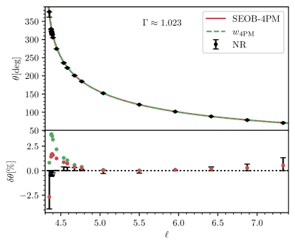
(a)

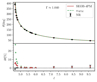
(b)

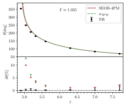
(c)

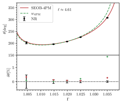
(d)

Figure 3: Comparison of the dissipative SEOB-4PM and $w_{\rm 4PM}$ models against the four equal-mass spinless NR data sets of Refs. [112, 111]. In each figure, the scattering angle $\theta$ (in degrees) is shown in the top panel, and the fractional difference $\delta\theta$ (49) in the lower panel. In the bottom-right figure, the energy $\Gamma$ is varied while the angular momentum $\ell$ is held fixed; vice versa in the other three figures. Both models show good agreement with NR, but this worsens in the strong-field regime near plunge (small $\ell$). The agreement also worsens for large energies with fixed angular momentum, particularly for the $w_{\rm PM}$ model.

Proceeding in this way to higher PM orders, we reconstruct all of the needed coefficients from the scattering angle. A complete set of results up to 4PM is provided in Appendix A, and up to 5PM (excluding the non-spinning component) in the attached ancillary file.

Starting at two-loop order (3PM in the non-spinning case), we may choose to insert either the conservative or full dissipative scattering angle into the model, as part of this matching procedure. We will examine both possibilities in the next section. In either case, the deformations also now include special functions of $\gamma$ that are inherited from the scattering angle: for example, ${\rm arccosh}\gamma$ when including two-loop results. At three-loop order (4PM in the non-spinning case), we also encounter logarithms and dilogarithms of rational functions of $\gamma$, plus the complete elliptic functions ${\rm K}({\textstyle\frac{\gamma-1}{\gamma+1}})$ and ${\rm E}({\textstyle\frac{\gamma-1}{\gamma+1}})$ of the first and second kind, respectively.

Lastly, we note that in the non-spinning limit, the conservative scattering angles of the SEOB-PM model coincide with the ones obtained in Ref. [95], since our model uses the PS* gauge. On the other hand, the dissipative effects differ from the ones of Ref. [95], because the latter included only the odd contributions following Ref. [145], since the even contributions were absent at the time the paper was published. In particular, working at linear order in the radiation reaction, the odd radiative contributions to the total scattering angle are estimated as half of the difference of the conservative scattering angle evaluated on the outgoing and incoming states (see the $H^{\rm EOB,PS*}_{\rm 4PM,hyp}$ model with and without odd dissipation in the right panels of Figs. 7 and 8 in Ref. [95]). Furthermore, the conservative scattering angle in Ref. [95] was computed by evolving the EOB Hamilton equations without the radiation-reaction force, and following the substitutions for $\gamma$ explained in the footnote 6. We will see below the impact of those differences when comparing the results of Ref. [95] with the SEOB-PM model and the NR data.

V EOB Scattering Angle and NR Comparisons

Let us now consider scattering angle predictions of the SEOB-PM model. In Sec. V.1 we compare these against angles computed from NR simulations of Refs. [111, 112] including also predictions of the $w_{\rm PM}$ model (16) of Refs. [113, 112]. Since both models can be expressed in terms of an effective potential $w(r)$ (11), given explicitly in Eq. (37b) and in Eq. (16), their predictions for the scattering angle are then given simply by (12):

$$\theta=-\pi-2\int^{\infty}_{r_{\rm min}}\mathrm{d}r\frac{\partial}{\partial L}\sqrt{p_{\infty}^{2}-\frac{L^{2}}{r^{2}}+w(E_{\rm eff},L,r;a_{\pm})}\,.$$ (48)

As stated above, $r_{\rm min}$ is the largest root of the equation $p_{r}=0$. Since the potentials depend on $r$ in quite general manners (in particular the SEOB-PM potential), the integral cannot easily be evaluated analytically. Thus, we simply evaluate this integral numerically to a sufficient degree of precision. The energy, angular momentum, masses and spins are fixed to values corresponding to the particular phase-space point under consideration.

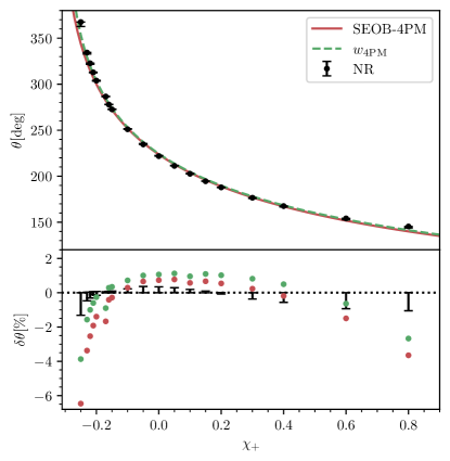
(a)

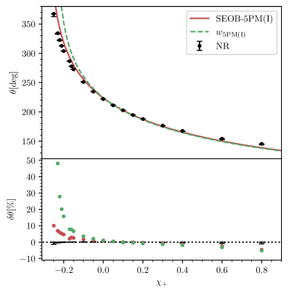
(b)

Figure 4: Comparisons with the equal-mass, equal-spins NR simulations of Ref. [112]. The top and lower panels show the absolute and fractional scattering angles respectively. The energy and angular momentum are kept approximately fixed with $\Gamma\approx 1.023$ and $\ell\approx 4.58$. On the left panel we show the SEOB-PM and $w_{\rm PM}$ models at 4PM order, and on the right panel at the incomplete 5PM order, since the non-spinning 5PM contributions are currently unknown.

Each model comprises a series of models corresponding to the kind of perturbative input given to the deformations. The most basic series of submodels here are the ones corresponding to a given PM order — where one may choose to include dissipative effects, or not. Below in Sec. V.2, however, we also explore the PN and spin expansions of these deformations. Here, we also compare the SEOB-PM and $w_{\rm PM}$ models for unequal masses $\nu\neq 1/4$. Finally, in Sec. V.3, we compute the critical angular momentum predicted by the SEOB-PM and $w_{\rm PM}$ models and analyze their effective potentials.

V.1 NR Comparisons

The available NR simulations for the scattering angles of two BHs are still rather limited, and are all restricted to equal masses. We consider here the three non-spinning series of simulations of Ref. [112] with varying angular momentum, and three fixed energies: $\Gamma\approx 1.023$, $\Gamma\approx 1.040$ and $\Gamma\approx 1.055$ (similar simulations with the first energy were first carried out in Ref. [110]). We consider also the single spinning series of simulations of Ref. [112] with varying (equal) dimensionless spins and fixed energy $\Gamma\approx 1.023$ and angular momentum $\ell\approx 4.58$. Finally, we consider the single non-spinning series of simulations of Ref. [111] with varying energy and fixed angular momentum $\ell\approx 4.61$.

In this section we focus on the models that include dissipation and compare those with the NR simulations. Thus, 4PM is the highest order at which the perturbative data is known and, also, the dissipative models agree much better than the conservative models with the NR data. The 4PM dissipative models explored here are therefore the most accurate models available. We explore the conservative part of the models below in Sec. V.2.

In Fig. 3, we compare the non-spinning SEOB-PM and $w_{\rm PM}$ models, at 4PM with dissipative effects, against the non-spinning NR data. Comparisons to the NR data for the $w_{\rm PM}$ model have already appeared in Refs. [113, 112] and our results are in full agreement. In each plot we show the SEOB-4PM and $w_{\rm 4PM}$ predictions across the relevant ranges of angular momentum or energy together with the NR simulation data points. In most of the phase space shown, the two models and the NR data lie very closely. In order to distinguish their behaviour, we also plot in each case the fractional difference $\delta\theta$:

$$\delta\theta=\frac{\theta_{\rm model}-\theta_{\rm NR}}{\theta_{\rm NR}}\ ,$$ (49)

where $\theta_{\rm model}$ is the angle computed either with the SEOB-4PM or $w_{\rm 4PM}$ models.

Generally the agreement between the models and NR data is rather remarkable: only in the strong field, near plunge does the relative difference rise to more than $10\%$. For the SEOB-4PM model, it never goes beyond $10\%$. When the models predict a plunge rather than scattering, no value for $\delta\theta$ is plotted. The performance of both the SEOB-4PM and $w_{\rm 4PM}$ models are good and comparable, though the relative difference of the SEOB-4PM model generally is smaller than that of $w_{\rm 4PM}$. This is evident in particular for the series of data at fixed angular momentum and varying energy in the bottom-right panel of Fig. 3.

In Fig. 4, we turn to the equal-mass, equal-spins simulations with constant energy and angular momentum, but varied spin. Here, we consider both the 4PM models (in the left panel) and incomplete 5PM models (5PM(I)) in the right panel). The incomplete 5PM model is defined by including all known information at 5PM (i.e. everything except the 4-loop spinless contribution, see Table 3).

Considering first the 4PM models in the left panel of Fig. 4, both models agree with the NR simulations within a relative difference of about $5\%$. It is, however, interesting that the agreement of both models worsens when the spin is increased. For positive spins, the scattering angle also decreases and one might have expected the models to perform better in this more perturbative regime (smaller angle). However, the positive spin becomes quite large, thus it seems desirable to improve the models in this phase space where the angles are not too big and should be describable. This could be achieved by including higher-spin terms beyond 4PM order (e.g., the tree-level $S^{4}$ or one-loop $S^{3}$) or exploring alternative deformations of the Kerr metric.

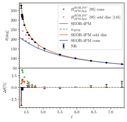
Figure 5: Relative importance of odd and even dissipative effects in the SEOB-4PM model. In addition, we compare the angles’ predictions of the SEOB-PM model here and in Ref. [95], where odd dissipative effects were incorporated with the radiation reaction of Ref. [145]. (We thank Mohammed Khalil for sharing with us the data, including the results of the last three data points in the strong field from Ref. [110] that were not included in Ref. [95].)

Considering, then, the incomplete 5PM models in the right panel of Fig. 4, we see that the agreement of the $w_{\rm PM}$ model with NR is significantly worse, reaching $50\%$. This, to a much lesser extent, is also true for the SEOB model, for which the difference with NR rises to about $10\%$. It will be interesting to see if the models improve once the genuine non-spinning 5PM contribution is computed. (We note that Ref. [112] improved the $w_{\rm PM}$ model by fitting the 5PM $S^{0}$ and 6PM $S^{1}$ terms to the NR scattering-angle data.)

V.2 Dependence on Dissipation, Perturbative Orders and Mass Ratio

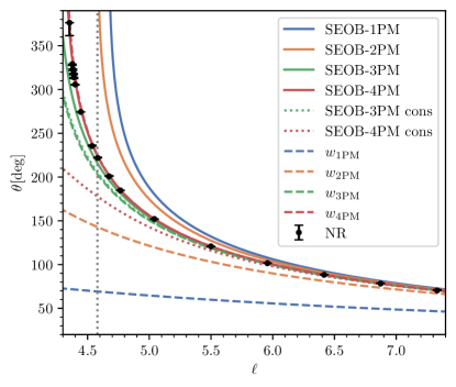
(a)

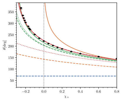
(b)

Figure 6: Analysis of the models at different PM orders, with or without dissipative effects. The energy is fixed $\Gamma\approx 1.023$: to the left $\ell$ is varied with fixed $\chi_{\pm}=0$, while to the right $\chi_{+}$ is varied with fixed $\ell\approx 4.58$ and $\chi_{-}=0$. The two plots share a single phase-space point marked with the vertical dotted grey lines. In the right plot, SEOB-1PM always predicts a plunge.

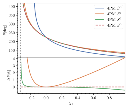
Figure 7: Analysis of importance of perturbative spin orders for the dissipative SEOB-4PM model. The kinematics is the same as the equal-mass, equal-spin NR simulations: $\Gamma\approx 1.023$ and $\ell\approx 4.58$. In the upper panel we plot SEOB-4PM angles omitting first all spin deformations (blue) and adding, then, successively linear (orange), quadratic (green) and cubic (red) spin deformations to the model. Starting from linear order in spins, the curves lie very near to each other and in the lower panel we plot their fractional difference to the (full) SEOB-4PM $S^{3}$ model. The vertical dotted line indicates the transition to plunge as predicted by the SEOB-4PM model. We note that this figure only compares its submodels, where certain spin deformations are omitted, with itself and not with the NR data.

Let us now analyze the importance of dissipation, and different PM, PN and spin orders. In Fig. 5 we compare the scattering angles of the full SEOB-4PM model (i.e., conservative plus odd and even dissipative) with the ones obtained by including only the odd dissipative terms. In accordance with Sec. II.2 (see also Eq. (26)), we find that, for the phase-space configurations for which we have NR data, the contribution to the scattering angle of the even dissipative terms is negligible, becoming more noticeable only in the strong field (see lower panel). We also compare the conservative scattering angles of the SEOB-4PM model with the ones of the EOB model of Ref. [95] (see the $H^{\rm EOB,PS*}_{\rm 4PM,hyp}$ model in Figs. 7 and 8 therein), which employed the same non-spinning PM Hamiltonian of this work, but computed the angles evolving the EOB Hamilton equations without the radiation-reaction force (see also the footnote 6). The two conservative predictions are very close. We also show the curve of Ref. [95] where the odd dissipative effects were included, following the method of Ref. [145]. (The even dissipative terms were not available at that time, and were later computed in Ref. [96].) We find that the estimation of the odd dissipative terms of Ref. [145] largely underestimate, at least for this phase-space configurations, the true odd dissipative contributions.

In Fig. 6 we plot scattering angle predictions of the SEOB-PM and $w_{\rm PM}$ models at 1, 2, 3 and 4PM orders. In addition, at 3PM and 4PM — where the conservative and dissipative models differ — we also plot the conservative SEOB-PM model predictions. Clearly, the dissipative effects have a large impact, as was already observed for the $w_{\rm PM}$ model [113, 112]. The dissipative 3PM and 4PM models are, however, sufficiently close to each other that one might hope for some sort of convergence. Interestingly, the SEOB-PM model converges from above in both cases (with an oscillatory behavior between the 3PM and 4PM order for the SEOB-PM model), in contrast to the $w_{\rm PM}$ which converges from below. Also, recall that the SEOB-PM model at 1PM encodes simply the probe limit. As seen in the right panel of Fig. 6, this motion uniformly predicts plunge, hence there is no SEOB-1PM curve. We note also that the $w_{\rm 1PM}$ curves may be computed with the formula given above in Eq. (18).

Next, in Fig. 7, we consider the importance of perturbative spin orders. Focusing on the SEOB-PM model at 4PM order, we omit progressively different orders of the spin corrections from the deformations. Thus, the models shown labeled by 4PM $S^{s}$ with $s=0,1,2,3$ denote a model where we include deformations $\alpha^{(n)}_{(i,j)}$ only with $n\leq 4$ and $(i+j)\leq s$. Thus, referring to Table 2, the model $s=0$ corresponds to the first column, the model $s=1$ corresponds to the first two columns, and so on up to 4PM order. The top panel shows the scattering angle and the lower panel shows fractional errors with respect to the genuine 4PM model (i.e., 4PM $S^{3}$). We define the fractional difference in this case by:

$$\Delta\theta=\frac{\theta_{\rm model}-\theta_{\rm SEOB-4PM}}{\theta_{\rm SEOB-4PM}},$$ (50)

where the subscript “model” could be any of the models 4PM $S^{s}$. From Fig. 7, it is clear that the spin-orbit $S^{1}$ corrections to the model are essential, while the contributions from higher spin orders are comparably much smaller. For larger values of the dimensionless spins, however, they do become relevant.

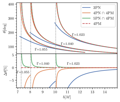
Figure 8: Analysis of importance of perturbative PN orders for the (dissipative) SEOB-PM model. Focusing on spinless, equal-mass dynamics, we consider three fixed energies $\Gamma=1.023$, $1.040$ and $1.055$ (corresponding to the velocities $v\approx 0.40$, $0.51$ and $0.58$) and vary the impact parameter (which is used instead of $\ell$ in order that the curves do not lie on top of each other). In the lower panel, the fractional difference of each PN approximation with respect to the 4PM model is shown. The vertical grey lines indicate the transition to plunge predicted by the 4PM model.

Let us then turn to PN contributions, and ask: is the all-order-in-$v$ PM information important or can a PN model describe the NR data equally well? Again, we focus on the SEOB-PM model and define a series of sub-models each of which contains only part of the information of the full 4PM model. Namely, we terminate the deformation parameters at a given PN order starting from 3PN and progressing to 5PN. Thus, generally, we may define a model $m\text{PN}\cap 4\text{PM}$ which includes all deformations until $m$PN order and 4PM order. Referring back to the right panel in Table 3, this corresponds to including all terms in the rectangle extending downwards to 4PM and to the right to $m$PN. We start from the model $3\text{PN}\cap 4\text{PM}=3\text{PN}$ and include the next two sub-leading orders in the comparison. Again, we compute a relative angle by comparing to the full 4PM model predictions just as in Eq. (50). Fig. 8 shows the comparison of the $m\text{PN}\cap 4\text{PM}$ against the 4PM model for $m=3,4,5$. Only at the sub-sub-leading order to 3PN does the velocity-expanded models keep in good agreement with the 4PM model all the way in the strong field, near to plunge. In the three data sets plotted in Fig. 8, one also notes that increasing the energy worsens the PN approximations.

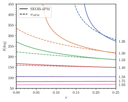
(a)

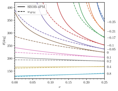
(b)

Figure 9: Predictions of the SEOB-4PM and $w_{\rm 4PM}$ models across the full range of symmetric mass ratios $0\leq\nu\leq 1/4$. In the left panel, the energy is $\Gamma=1.055$ and the spins vanish $\chi_{\pm}=0$; the numbers along the right vertical axis indicate values of $\ell$ for the different curves. In the right panel, $\Gamma=1.023$, $\ell=4.58$, $\chi_{-}=0$, and the numbers along the right vertical axis indicate values of $\chi_{+}$ for the different curves. Note that for unequal masses there is recoil, and thus a (slight) difference between $\theta_{1}$, $\theta_{2}$ and $\theta_{\rm rel}$. The curves shown here are modelled around $\theta_{\rm rel}$ (as discussed in Sec. II.2).

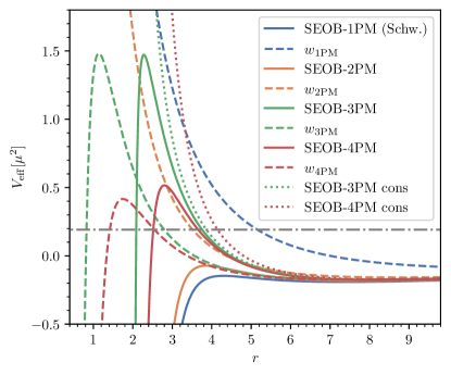
Figure 10: For each model we plot the effective potential $V_{\rm eff}(r)$ defined from the radial action as $p_{r}^{2}=p_{\infty}^{2}-V_{\rm eff}(r)$. The phase space point is equal-mass, non-spinning with $\Gamma=1.02264$ and $\ell=4.4$. The grey dash-dotted straight line indicates the corresponding value of $p_{\infty}^{2}$: a model predicts plunge if the potential never rises beyond that line. The effective potentials depend on the kinematics and the condition for the critical angular momentum is that the peak of the potential (if it exists) touches the line of $p_{\infty}^{2}$.

Finally, we consider the mass dependence of the two models SEOB-PM and $w_{\rm PM}$. Naturally, the SEOB-PM model is designed to describe exactly the probe limit $\nu\to 0$ and $a_{+}=a_{-}$, which is a feature not included in the $w_{\rm PM}$ model. In Fig. 9 we plot angle predictions of the two models across the whole range of $0\leq\nu\leq 1/4$. We do so for the phase-space points of two of the NR data sets. First, in the left panel, we do so for each value of $\ell$ of the third series of NR data of Ref. [112] with fixed energy $\Gamma\approx 1.055$. Second, in the right panel, we do so for a selection of the equal-spins simulations of Ref. [112].

As we already saw above, the two models give relatively similar results in the $\nu=1/4$ regime. As seen in Fig. 9 this, however, is generally not the case for smaller mass ratios. Thus, for increasing scattering angles, the two models begin to differ more and more for mass ratios $\nu\neq 1/4$. By design, the leftmost $\nu\to 0$ prediction of the SEOB-PM model in the left panel of Fig. 9 is exact. This is not the case for the right panel, as that would require a vanishing spin on the probe. As an example, for $\ell\approx 1.30$ in the left panel, $w_{\rm PM}$ predicts a finite angle in this limit while probe motion would predict a plunge.

On the other hand, for smaller scattering angles the curves are more or less insensitive to the changing mass ratio. This is in good agreement with the fact that the 1PM and 2PM perturbative scattering angles essentially are independent of $\nu$ (except for too large energies). It will be very important to produce NR simulations of scattering BHs for a variety of mass ratios and spins, so that those models can be validated much more broadly. We also remark that for the unequal masses considered in Fig. 9, recoil effects will be non-zero and the scattering angles $\theta_{1}$, $\theta_{2}$ and $\theta_{\rm rel}$ are different. While we have no NR data to compare with, one may think of the predictions shown there as referring to $\theta_{\rm rel}$ (which can also be extracted from NR simulations if the impulses $\Delta p_{i}$ are known).

V.3 Importance of the Critical Angular Momentum

An essential feature of the non-perturbative dynamics is the possibility of a plunge for small values of the angular momentum $\ell$. Thus, if one fixes all variables but $\ell$, there is a critical value denoted by $\ell_{0}$ for which the orbital motion goes from scattering to plunge. This scenario is ideally explored in the three panels of Fig. 3 with fixed energy (using the NR data of Ref. [112]). Here, the NR data explores this limit where the curve meets a vertical asymptote (i.e. $\ell_{0}$). In fact, every series of NR data was terminated only after a plunge was ascertained for a given value of $\ell$ (see, e.g., the tables in Appendix B). In each of the three cases, with the energies $\Gamma_{1}=1.02264$, $\Gamma_{2}=1.04033$ and $\Gamma_{3}=1.05548$, one may therefore bound the critical angular momentum:

$$4.3076 \leq\ell_{0}(\Gamma_{1})\leq 4.3536\ ,$$ (51a)

$$4.602 \leq\ell_{0}(\Gamma_{2})\leq 4.638\ ,$$ (51b)

$$4.2 \leq\ell_{0}(\Gamma_{3})\leq 4.9\ .$$ (51c)

The bound for the third energy, however, is very wide.

The accuracy of an analytical model in the strong field greatly depends on its ability to predict the critical angular momentum. Its appearance may be gathered from the shapes of the effective potentials $V_{\rm eff}=p_{\infty}^{2}-p_{r}^{2}$ of the models plotted in Fig. 10. These shapes are characteristic of the effective potential of BH metrics (i.e., the SEOB-1PM curve in Fig. 10). The plunge (or inspiral) happens when there is no longer a barrier generated by the potential. In other words, when the grey dash-dotted line is never crossed by the potentials. The critical point of transition from scattering to plunge is then determined by the potential touching the grey dash-dotted line just once. In other words, $p_{r}(r_{\rm min})=0$ and $\partial p_{r}(r_{\rm min})/\partial r=0$. For the three energies $\Gamma_{i}$ we determine the critical angular momenta predicted by the dissipative SEOB-4PM and $w_{\rm 4PM}$ models to be:

$$\ell_{0}^{\rm SEOB-4PM}(\Gamma_{1}) =4.3046, \ell_{0}^{\rm wPM}(\Gamma_{1})=4.3148,$$ (52a)

$$\ell_{0}^{\rm SEOB-4PM}(\Gamma_{2}) =4.6089, \ell_{0}^{\rm wPM}(\Gamma_{2})=4.6439,$$ (52b)

$$\ell_{0}^{\rm SEOB-4PM}(\Gamma_{3}) =4.9072, \ell_{0}^{\rm wPM}(\Gamma_{3})=4.9272,$$ (52c)

Generally, these values lie within or near the bounds given in Eqs. (51).

VI Conclusions

Building on earlier work [91, 92, 93, 94, 95, 49], we have derived the spinning EOB Hamiltonian SEOB-PM that resums PM perturbative calculations fully through 4PM order, and at 5PM where results are known. Our PM counting is a physical one, with both loop and spin orders contributing; thus, both three-loop spin-orbit [108, 109] and two-loop spin-squared [105, 106, 107] scattering results contribute to the model at 5PM order. The SEOB-PM Hamiltonian includes nonlocal-in-time (tail) contributions for unbound orbits, and thus fully describes hyperbolic trajectories. We have employed the SEOB-PM model to compute resummed conservative scattering angles for non-spinnning and spinning BHs, and, after accounting for dissipative contributions, we have compared the total scattering angles to the NR data of Refs. [111, 112]. We have also compared SEOB-PM results with the $w_{\rm PM}$-potential–model predictions in those papers (therein referred to as $w_{\rm EOB}$), which can be viewed as a PM-expanded version of our $w_{\rm SEOB-PM}$-potential model.

We find that the performance of both the SEOB-PM and $w_{\rm PM}$ models are very good and comparable, though the fractional difference of the SEOB-PM model to NR is generally slightly smaller than that of $w_{\rm PM}$. This is evident in particular for the set of scattering angles at fixed angular momentum and varying energy, toward larger energy, and also when comparing to NR data the models at the (incomplete) 5PM order. However, the NR data here is so limited that we cannot draw from these few examples any definitive conclusions. In fact, in the region of parameter space where we expect the two models to differ the most, notably toward the probe limit (i.e. symmetric mass ratio different from 1/4), we do not have any NR data. Nevertheless, we stress that whereas the SEOB-PM model (by construction) reduces to the $w$-potential and Hamiltonian of a test-mass in the Schwarzschild or Kerr spacetime, this is not the case for the $w_{\rm PM}$ model.

Similarly to what was found for the $w_{\rm PM}$ model in Ref. [112], when comparing to spinning NR data for equal-mass BHs, SEOB-PM performs worse when spins are aligned with the angular momentum and the spin magnitude increases. Although in this case, the scattering angles are small, thus in the weak-field region, the models are not yet sufficiently accurate. This motivates the need to complete $G^{5}$ by computing the non-spinning 5PM scattering dynamics. We also found that including radiative (dissipative) effects is also necessary for achieving a good agreement with NR; though, the odd dissipation plays a significantly more important role than the even one.

The resummed conservative scattering-angle results that we derived here were obtained from an EOB Hamiltonian. Thus, our SEOB-PM model has the advantage that it can be tested also for bound orbits and it can be used to construct waveform models. Indeed, Ref. [114] is already employing the SEOB-PM Hamiltonian at 4PM, augmented with known local-in-time contributions at 4PN order for bound orbits [115, 116, 117, 118, 119], to produce waveform models for spinning BHs on quasi-circular orbits.

Appendix A SEOB-PM Deformation Coefficients

In this appendix we present the deformations required to fully specify the SEOB-PM model up to physical 4PM order, as a function of the scattering angle (13a). No deformations are required at 1PM order; results up to 2PM are provided in the main text (45). At 3PM, we require results up to quadratic in spin:

$$\alpha^{(3)}_{(0,0)} =\frac{12\left(6\gamma^{4}-11\gamma^{2}+5\right)\theta^{(2)}_{(0,0)}+\pi\left(-142\gamma^{6}+309\gamma^{4}-3\gamma^{2}(\theta^{(3)}_{(0,0)}v_{\infty}+68)+3\theta^{(3)}_{(0,0)}v_{\infty}+35\right)}{6\pi\gamma^{2}v_{\infty}^{4}}\,,$$ (53a)

$$\alpha^{(3)}_{(1,0)} =\frac{\pi\left(5\gamma^{2}-3\right)\theta^{(2)}_{(1,0)}-2\theta^{(3)}_{(1,0)}v_{\infty}}{2\pi\gamma v_{\infty}^{3}}\,,\qquad\alpha^{(3)}_{(0,1)}=\frac{\pi\left(5\gamma^{2}-3\right)\theta^{(2)}_{(0,1)}-2\theta^{(3)}_{(0,1)}v_{\infty}}{2\pi\gamma v_{\infty}^{3}}\,,$$ (53b)

$$\alpha^{(3)}_{(2,0)} =\frac{2\gamma^{2}-1}{\gamma^{2}}-\frac{\theta^{(3)}_{(2,0)}}{2\gamma^{2}v_{\infty}}\,,\qquad\alpha^{(3)}_{(1,1)}=-\frac{\theta^{(3)}_{(1,1)}}{2\gamma^{2}v_{\infty}}\,,\qquad\alpha^{(3)}_{(0,2)}=-\frac{\theta^{(3)}_{(0,2)}}{2\gamma^{2}v_{\infty}}\,,$$ (53c)

where $v_{\infty}=\sqrt{\gamma^{2}-1}$. At 4PM our results go up to cubic order in spins:

$$\alpha^{(4)}_{(0,0)} =\frac{1}{48\pi^{2}\gamma^{4}v_{\infty}^{6}}\bigg{(}96v_{\infty}^{4}\left(3\gamma^{2}-2\right)(\theta^{(2)}_{(0,0)})^{2}-32\pi v_{\infty}^{2}\left(2v_{\infty}^{2}\gamma^{2}\theta^{(4)}_{(0,0)}+3\left(33\gamma^{6}-58\gamma^{4}+30\gamma^{2}-3\right)\theta^{(2)}_{(0,0)}\right)$$ (54a)

$$+\pi^{2}\left(4127\gamma^{10}-12976\gamma^{8}+42\gamma^{6}(4\theta^{(3)}_{(0,0)}v_{\infty}+365)-4\gamma^{4}(72\theta^{(3)}_{(0,0)}v_{\infty}+2011)+\gamma^{2}(120\theta^{(3)}_{(0,0)}v_{\infty}+1703)-108\right)\bigg{)}\,,$$

$$\alpha^{(4)}_{(1,0)} =\frac{4\left(5\gamma^{4}-7\gamma^{2}+2\right)\theta^{(2)}_{(0,0)}\theta^{(2)}_{(1,0)}-2\pi v_{\infty}^{2}\gamma^{2}\theta^{(4)}_{(1,0)}+\pi\left(-99\gamma^{6}+132\gamma^{4}-57\gamma^{2}+6\right)\theta^{(2)}_{(1,0)}+24\left(2\gamma^{2}-1\right)\gamma^{2}\theta^{(3)}_{(1,0)}v_{\infty}}{8\pi\gamma^{3}v_{\infty}^{5}}\,,$$ (54b)

$$\alpha^{(4)}_{(0,1)} =\frac{4\left(5\gamma^{4}-7\gamma^{2}+2\right)\theta^{(2)}_{(0,0)}\theta^{(2)}_{(0,1)}-2\pi v_{\infty}^{2}\gamma^{2}\theta^{(4)}_{(0,1)}+\pi\left(-99\gamma^{6}+132\gamma^{4}-57\gamma^{2}+6\right)\theta^{(2)}_{(0,1)}+24\left(2\gamma^{2}-1\right)\gamma^{2}\theta^{(3)}_{(0,1)}v_{\infty}}{8\pi\gamma^{3}v_{\infty}^{5}}\,,$$ (54c)

$$\alpha^{(4)}_{(2,0)} =-\frac{3\pi\left(v_{\infty}\left(84\gamma^{6}-152\gamma^{4}+\gamma^{2}\left(68-15(\theta^{(2)}_{(1,0)})^{2}\right)+3(\theta^{(2)}_{(1,0)})^{2}\right)+8\left(5-7\gamma^{2}\right)\gamma^{2}\theta^{(3)}_{(2,0)}\right)+64\gamma^{2}\theta^{(4)}_{(2,0)}v_{\infty}}{48\pi\gamma^{4}v_{\infty}^{3}}\,,$$ (54d)

$$\alpha^{(4)}_{(1,1)} =\frac{9\pi\left(5\gamma^{2}-1\right)\theta^{(2)}_{(0,1)}\theta^{(2)}_{(1,0)}v_{\infty}+12\pi\left(7\gamma^{2}-5\right)\gamma^{2}\theta^{(3)}_{(1,1)}-32\gamma^{2}\theta^{(4)}_{(1,1)}v_{\infty}}{24\pi\gamma^{4}v_{\infty}^{3}}\,,$$ (54e)

$$\alpha^{(4)}_{(0,2)} =\frac{9\pi\left(5\gamma^{2}-1\right)\delta^{2}(\theta^{(2)}_{(0,1)})^{2}v_{\infty}+24\pi\left(7\gamma^{2}-5\right)\gamma^{2}\theta^{(3)}_{(0,2)}-64\gamma^{2}\theta^{(4)}_{(0,2)}v_{\infty}}{48\pi\gamma^{4}v_{\infty}^{3}}\,,$$ (54f)

$$\alpha^{(4)}_{(3,0)} =\frac{v_{\infty}^{2}\theta^{(2)}_{(1,0)}-\theta^{(4)}_{(3,0)}}{4\gamma v_{\infty}^{3}}\,,\,\alpha^{(4)}_{(2,1)}=\frac{v_{\infty}^{2}\theta^{(2)}_{(0,1)}-\theta^{(4)}_{(2,1)}}{4\gamma v_{\infty}^{3}}\,,\,\alpha^{(4)}_{(1,2)}=-\frac{\theta^{(4)}_{(1,2)}}{4\gamma v_{\infty}^{3}}\,,\,\alpha^{(4)}_{(0,3)}=-\frac{\theta^{(4)}_{(0,3)}}{4\gamma v_{\infty}^{3}}\,.$$ (54g)

Inserting the scattering-angle coefficients $\theta_{(i,j)}^{(n)}$, in either the conservative or dissipative, yields the full coefficients. These are provided in the ancillary file attached to the arXiv submission of this paper up to 5PM order, plus a 6PM term at quartic order in spins ($S^{4}$).

Appendix B Scattering angles

In this appendix we list the data for the NR simulations, as well, as the scattering-angle predictions for the models considered in this paper. We indicate a plunge (or prediction thereof) with a minus, “$-$”. We always show the angle in degrees with the fractional uncertainty in percentage in brackets. We note that for the Tables 4, 6 and 7, Ref. [112] reported an uncertainty in whether the final scattering simulation before plunge, could also have been a plunge.

NR data			SEOB-4PM	$w_{\rm 4PM}$	SEOB-5PM(I)	$w_{\rm 5PM(I)}$
$\chi_{+}$	$\Gamma$	$\theta[{\rm deg}]$	$\theta[{\rm deg}](\delta\theta[\%])$	$\theta[{\rm deg}](\delta\theta[\%])$	$\theta[{\rm deg}](\delta\theta[\%])$	$\theta[{\rm deg}](\delta\theta[\%])$
-0.3	1.02269	$-$	444.865	521.326	$-$	$-$
-0.25	1.02268	$367.545^{+0.}_{-4.84}$	343.778 (-6.5)	353.322 (-3.9)	404.532 (10.1)	$-$
-0.23	1.02267	$334.345^{+0.084}_{-1.573}$	323.065 (-3.4)	329.103 (-1.6)	357.495 (6.9)	495.03 (48.1)
-0.22	1.02267	$322.693^{+0.099}_{-1.004}$	314.512 (-2.5)	319.468 (-1.)	341.921 (6.)	412.428 (27.8)
-0.21	1.02267	$312.795^{+0.187}_{-0.364}$	306.799 (-1.9)	310.926 (-0.6)	329.068 (5.2)	375.805 (20.1)
-0.2	1.02266	$303.884^{+0.222}_{-0.466}$	299.644 (-1.4)	303.102 (-0.3)	317.95 (4.6)	351.697 (15.7)
-0.17	1.02266	$286.603^{+0.154}_{-0.01}$	281.815 (-1.7)	284.027 (-0.9)	292.662 (2.1)	309.066 (7.8)
-0.16	1.02266	$277.849^{+0.23}_{-0.003}$	276.702 (-0.4)	278.644 (0.3)	285.91 (2.9)	299.349 (7.7)
-0.15	1.02265	$272.603^{+0.26}_{-0.003}$	271.827 (-0.3)	273.537 (0.3)	279.648 (2.6)	290.746 (6.7)
-0.1	1.02265	$251.028^{+0.559}_{-0.003}$	251.762 (0.3)	252.829 (0.7)	255.221 (1.7)	260.003 (3.6)
-0.05	1.02264	$234.568^{+0.845}_{-0.003}$	236.109 (0.7)	236.923 (1.)	237.352 (1.2)	239.441 (2.1)
0.	1.02264	$221.823^{+0.762}_{-0.002}$	223.442 (0.7)	224.179 (1.1)	223.442 (0.7)	224.179 (1.1)
0.05	1.02264	$211.195^{+0.61}_{-0.002}$	212.83 (0.8)	213.568 (1.1)	212.089 (0.4)	212.078 (0.4)
0.1	1.02265	$202.608^{+0.388}_{-0.002}$	203.765 (0.6)	204.545 (1.)	202.568 (0.)	202.123 (-0.2)
0.15	1.02265	$194.542^{+0.183}_{-0.001}$	195.838 (0.7)	196.673 (1.1)	194.359 (-0.1)	193.654 (-0.5)
0.2	1.02266	$187.838^{+0.02}_{-0.141}$	188.854 (0.5)	189.753 (1.)	187.203 (-0.3)	186.344 (-0.8)
0.3	1.02269	$176.586^{+0.001}_{-0.653}$	176.997 (0.2)	178.026 (0.8)	175.197 (-0.8)	174.202 (-1.4)
0.4	1.02274	$167.545^{+0.002}_{-0.941}$	167.228 (-0.2)	168.374 (0.5)	165.423 (-1.3)	164.405 (-1.9)
0.6	1.02288	$154.139^{+0.005}_{-1.443}$	151.833 (-1.5)	153.156 (-0.6)	150.206 (-2.6)	149.265 (-3.2)
0.8	1.02309	$145.357^{+0.006}_{-1.528}$	140.053 (-3.6)	141.474 (-2.7)	138.705 (-4.6)	137.879 (-5.1)

Table 4: Spinning NR data of Ref. [112] and model predictions. The following variables are constant across all data points: $\chi_{-}=0$ and $\ell=4.5824$.

      

      

NR data			SEOB-4PM	$w_{\rm PM}$
$\Gamma$	$\ell$	$\theta_{\rm NR}[{\rm deg}]$	$\theta[{\rm deg}](\delta\theta(\%))$	$\theta[{\rm deg}](\delta\theta(\%))$
1.00457	4.608	$201.9^{+4.8}_{-4.8}$	205.227 (1.6)	202.688 (0.4)
1.01479	4.6077	$195.9^{+1.3}_{-1.3}$	197.077 (0.6)	196.008 (0.1)
1.01988	4.6076	$207.03^{+0.99}_{-0.99}$	207.849 (0.4)	207.683 (0.3)
1.02496	4.6074	$225.54^{+0.87}_{-0.87}$	226.256 (0.3)	227.839 (1.)
1.03503	4.6061	$307.13^{+0.88}_{-0.88}$	311.297 (1.4)	334.271 (8.8)

Table 5: Equal-mass, spinless series of NR data from Ref. [111]. The angular momentum is approximately fixed. The values of $\Gamma$ and $\ell$ reported here are rounded off. For computations, we have used the values reported in Table II of Ref. [111]. The $w_{\rm 4PM}$ angles agree with those reported in Ref. [113].

NR data		SEOB-4PM	$w_{\rm 4PM}$
$\ell$	$\theta[{\rm deg}]$	$\theta[{\rm deg}](\delta\theta[\%])$	$\theta[{\rm deg}](\delta\theta[\%])$
4.3076	$-$	609.322($-$)	$-$
4.3536	$376.275^{+0.026}_{-14.69}$	366.188 (-2.7)	379.31 (0.8)
4.3764	$329.057^{+0.003}_{-1.534}$	333.711 (1.4)	341.135 (3.7)
4.3808	$323.422^{+0.}_{-1.914}$	328.694 (1.6)	335.476 (3.7)
4.3856	$318.394^{+0.}_{-1.575}$	323.552 (1.6)	329.728 (3.6)
4.39	$313.764^{+0.}_{-1.331}$	319.111 (1.7)	324.803 (3.5)
4.3992	$305.734^{+0.056}_{-0.694}$	310.548 (1.6)	315.401 (3.2)
4.4452	$274.368^{+0.074}_{-0.016}$	277.789 (1.2)	280.337 (2.2)
4.5368	$235.447^{+0.912}_{-0.003}$	237.465 (0.9)	238.507 (1.3)
4.5824	$221.823^{+0.762}_{-0.002}$	223.442 (0.7)	224.179 (1.1)
4.6744	$200.81^{+0.62}_{-0.004}$	201.581 (0.4)	201.991 (0.6)
4.766	$184.684^{+0.221}_{-0.002}$	185.16 (0.3)	185.411 (0.4)
5.0408	$152.106^{+0.055}_{-0.446}$	152.15 (0.)	152.231 (0.1)
5.4992	$120.804^{+0.013}_{-0.307}$	120.8 (0.)	120.821 (0.)
5.9572	$101.616^{+0.059}_{-0.002}$	101.696 (0.1)	101.704 (0.1)
6.4156	$88.26^{+0.337}_{-0.002}$	88.42 (0.2)	88.423 (0.2)
6.874	$78.296^{+0.52}_{-0.002}$	78.514 (0.3)	78.515 (0.3)
7.332	$70.404^{+0.927}_{-0.003}$	70.776 (0.5)	70.777 (0.5)

Table 6: First equal-mass, spinless series of NR data from Ref. [112] and model predictions. The $w_{\rm 4PM}$ predictions computed here are identical to the ones given in Ref. [112]. The energy is fixed with $\Gamma=1.02264$.

NR data		SEOB-4PM	$w_{\rm 4PM}$
$\ell$	$\theta[{\rm deg}]$	$\theta[{\rm deg}](\delta\theta(\%))$	$\theta[{\rm deg}](\delta\theta(\%))$
4.602	$-$	$-$	$-$
4.638	$392.815^{+0.006}_{-7.477}$	413.403 (5.2)	$-$
4.662	$338.973^{+0.156}_{-0.756}$	359.875 (6.2)	430.914 (27.1)
4.68	$317.637^{+0.142}_{-0.444}$	334.244 (5.2)	374.716 (18.)
4.722	$283.359^{+0.343}_{-0.007}$	294.155 (3.8)	312.437 (10.3)
4.758	$262.825^{+0.749}_{-0.008}$	270.784 (3.)	282.302 (7.4)
4.8	$244.21^{+1.22}_{-0.005}$	250.183 (2.4)	257.74 (5.5)
5.04	$184.138^{+0.439}_{-0.004}$	186.039 (1.)	187.734 (2.)
5.28	$153.119^{+0.226}_{-0.227}$	153.934 (0.5)	154.603 (1.)
5.4	$141.986^{+0.244}_{-0.213}$	142.634 (0.5)	143.094 (0.8)
5.64	$124.805^{+0.154}_{-0.238}$	125.244 (0.4)	125.487 (0.5)
5.7	$121.233^{+0.18}_{-0.153}$	121.669 (0.4)	121.88 (0.5)
5.76	$117.897^{+0.157}_{-0.091}$	118.333 (0.4)	118.517 (0.5)
6.	$106.459^{+0.207}_{-0.004}$	106.904 (0.4)	107.016 (0.5)
7.2	$73.095^{+1.358}_{-0.006}$	73.808 (1.)	73.826 (1.)
8.4	$56.489^{+1.242}_{-0.006}$	57.155 (1.2)	57.16 (1.2)
9.6	$45.982^{+1.53}_{-0.008}$	46.866 (1.9)	46.868 (1.9)

Table 7: Second equal-mass, spinless series of NR data from Ref. [112] and model predictions. The $w_{\rm 4PM}$ predictions computed here are identical to the ones given in Ref. [112]. The energy is fixed with $\Gamma=1.04033$.

NR data		SEOB-4PM	$w_{\rm 4PM}$
$\ell$	$\theta[{\rm deg}]$	$\theta[{\rm deg}](\delta\theta(\%))$	$\theta[{\rm deg}](\delta\theta(\%))$
4.2	$-$	$-$	$-$
4.9	$354.118^{+0.307}_{-0.633}$	$-$	$-$
5.04	$248.95^{+1.203}_{-0.005}$	273.639 (9.9)	280.445 (12.7)
5.18	$206.064^{+1.479}_{-0.006}$	216.687 (5.2)	218.732 (6.1)
5.32	$179.815^{+0.484}_{-0.006}$	185.602 (3.2)	186.552 (3.7)
5.6	$146.516^{+0.354}_{-0.096}$	149.089 (1.8)	149.418 (2.)
6.3	$104.166^{+0.361}_{-0.006}$	105.225 (1.)	105.287 (1.1)
7.	$82.275^{+0.924}_{-0.007}$	83.171 (1.1)	83.191 (1.1)
7.7	$68.351^{+1.485}_{-0.007}$	69.33 (1.4)	69.339 (1.4)

Table 8: Third equal-mass, spinless series of NR data from Ref. [112] and model predictions. The $w_{\rm 4PM}$ predictions computed here are identical to the ones given in Ref. [112]. The energy is fixed with $\Gamma=1.05548$.

References

- [1] LIGO Scientific, Virgo collaboration, B. Abbott et al., Observation of Gravitational Waves from a Binary Black Hole Merger, Phys. Rev. Lett. 116 (2016) 061102 [1602.03837].
- [2] LIGO Scientific, Virgo collaboration, B. P. Abbott et al., GW170817: Observation of Gravitational Waves from a Binary Neutron Star Inspiral, Phys. Rev. Lett. 119 (2017) 161101 [1710.05832].
- [3] LIGO Scientific, Virgo collaboration, B. P. Abbott et al., GW170817: Measurements of neutron star radii and equation of state, Phys. Rev. Lett. 121 (2018) 161101 [1805.11581].
- [4] LIGO Scientific, VIRGO, KAGRA collaboration, R. Abbott et al., Tests of General Relativity with GWTC-3, 2112.06861.
- [5] LIGO Scientific, Virgo, KAGRA collaboration, R. Abbott et al., Constraints on the Cosmic Expansion History from GWTC–3, Astrophys. J. 949 (2023) 76 [2111.03604].
- [6] KAGRA, VIRGO, LIGO Scientific collaboration, R. Abbott et al., GWTC-3: Compact Binary Coalescences Observed by LIGO and Virgo during the Second Part of the Third Observing Run, Phys. Rev. X 13 (2023) 041039 [2111.03606].
- [7] A. H. Nitz, S. Kumar, Y.-F. Wang, S. Kastha, S. Wu, M. Schäfer et al., 4-OGC: Catalog of Gravitational Waves from Compact Binary Mergers, Astrophys. J. 946 (2023) 59 [2112.06878].
- [8] D. Wadekar, J. Roulet, T. Venumadhav, A. K. Mehta, B. Zackay, J. Mushkin et al., New black hole mergers in the LIGO-Virgo O3 data from a gravitational wave search including higher-order harmonics, 2312.06631.
- [9] KAGRA, VIRGO, LIGO Scientific collaboration, R. Abbott et al., Population of Merging Compact Binaries Inferred Using Gravitational Waves through GWTC-3, Phys. Rev. X 13 (2023) 011048 [2111.03634].
- [10] T. Futamase and Y. Itoh, The post-Newtonian approximation for relativistic compact binaries, Living Rev. Rel. 10 (2007) 2.
- [11] L. Blanchet, Gravitational Radiation from Post-Newtonian Sources and Inspiralling Compact Binaries, Living Rev. Rel. 17 (2014) 2 [1310.1528].
- [12] R. A. Porto, The effective field theorist’s approach to gravitational dynamics, Phys. Rept. 633 (2016) 1 [1601.04914].
- [13] Schäfer, Gerhard and Jaranowski, Piotr, Hamiltonian formulation of general relativity and post-Newtonian dynamics of compact binaries, Living Rev. Rel. 21 (2018) 7 [1805.07240].
- [14] M. Levi, Effective Field Theories of Post-Newtonian Gravity: A comprehensive review, Rept. Prog. Phys. 83 (2020) 075901 [1807.01699].
- [15] K. Westpfahl and M. Goller, Gravitational scattering of two relativistic particles in postlinear approximation, Lett. Nuovo Cim. 26 (1979) 573.
- [16] K. Westpfahl and H. Hoyler, Gravitational bremsstrahlung in post-linear fast-motion approximation, Lett. Nuovo Cim. 27 (1980) 581.
- [17] L. Bel, T. Damour, N. Deruelle, J. Ibanez and J. Martin, Poincaré-invariant gravitational field and equations of motion of two pointlike objects: The postlinear approximation of general relativity, Gen. Rel. Grav. 13 (1981) 963.
- [18] K. Westpfahl, High-Speed Scattering of Charged and Uncharged Particles in General Relativity, Fortsch. Phys. 33 (1985) 417.
- [19] G. Schäfer, The adm hamiltonian at the postlinear approximation, General relativity and gravitation 18 (1986) 255.
- [20] T. Ledvinka, G. Schaefer and J. Bicak, Relativistic Closed-Form Hamiltonian for Many-Body Gravitating Systems in the Post-Minkowskian Approximation, Phys. Rev. Lett. 100 (2008) 251101 [0807.0214].
- [21] T. Damour, Gravitational scattering, post-Minkowskian approximation and Effective One-Body theory, Phys. Rev. D94 (2016) 104015 [1609.00354].
- [22] C. Cheung, I. Z. Rothstein and M. P. Solon, From Scattering Amplitudes to Classical Potentials in the Post-Minkowskian Expansion, Phys. Rev. Lett. 121 (2018) 251101 [1808.02489].
- [23] Z. Bern, C. Cheung, R. Roiban, C.-H. Shen, M. P. Solon and M. Zeng, Scattering Amplitudes and the Conservative Hamiltonian for Binary Systems at Third Post-Minkowskian Order, Phys. Rev. Lett. 122 (2019) 201603 [1901.04424].
- [24] A. Buonanno, M. Khalil, D. O’Connell, R. Roiban, M. P. Solon and M. Zeng, Snowmass White Paper: Gravitational Waves and Scattering Amplitudes, in 2022 Snowmass Summer Study, 4, 2022, 2204.05194.
- [25] Y. Mino, M. Sasaki and T. Tanaka, Gravitational radiation reaction to a particle motion, Phys. Rev. D 55 (1997) 3457 [gr-qc/9606018].
- [26] T. C. Quinn and R. M. Wald, An Axiomatic approach to electromagnetic and gravitational radiation reaction of particles in curved space-time, Phys. Rev. D 56 (1997) 3381 [gr-qc/9610053].
- [27] L. Barack, Y. Mino, H. Nakano, A. Ori and M. Sasaki, Calculating the gravitational selfforce in Schwarzschild space-time, Phys. Rev. Lett. 88 (2002) 091101 [gr-qc/0111001].
- [28] L. Barack and A. Ori, Gravitational selfforce on a particle orbiting a Kerr black hole, Phys. Rev. Lett. 90 (2003) 111101 [gr-qc/0212103].
- [29] S. E. Gralla and R. M. Wald, A Rigorous Derivation of Gravitational Self-force, Class. Quant. Grav. 25 (2008) 205009 [0806.3293].
- [30] S. L. Detweiler, A Consequence of the gravitational self-force for circular orbits of the Schwarzschild geometry, Phys. Rev. D77 (2008) 124026 [0804.3529].
- [31] T. S. Keidl, A. G. Shah, J. L. Friedman, D.-H. Kim and L. R. Price, Gravitational Self-force in a Radiation Gauge, Phys. Rev. D 82 (2010) 124012 [1004.2276].
- [32] M. van de Meent, Gravitational self-force on generic bound geodesics in Kerr spacetime, Phys. Rev. D 97 (2018) 104033 [1711.09607].
- [33] A. Pound, Second-order gravitational self-force, Phys. Rev. Lett. 109 (2012) 051101 [1201.5089].
- [34] A. Pound, B. Wardell, N. Warburton and J. Miller, Second-order self-force calculation of the gravitational binding energy in compact binaries, Phys. Rev. Lett. 124 (2020) 021101 [1908.07419].
- [35] S. E. Gralla and K. Lobo, Self-force effects in post-Minkowskian scattering, Class. Quant. Grav. 39 (2022) 095001 [2110.08681].
- [36] A. Pound and B. Wardell, Black hole perturbation theory and gravitational self-force, 2101.04592.
- [37] N. Warburton, A. Pound, B. Wardell, J. Miller and L. Durkan, Gravitational-Wave Energy Flux for Compact Binaries through Second Order in the Mass Ratio, Phys. Rev. Lett. 127 (2021) 151102 [2107.01298].
- [38] F. Pretorius, Evolution of binary black hole spacetimes, Phys. Rev. Lett. 95 (2005) 121101 [gr-qc/0507014].
- [39] M. Campanelli, C. O. Lousto, P. Marronetti and Y. Zlochower, Accurate evolutions of orbiting black-hole binaries without excision, Phys. Rev. Lett. 96 (2006) 111101 [gr-qc/0511048].
- [40] J. G. Baker, J. Centrella, D.-I. Choi, M. Koppitz and J. van Meter, Gravitational wave extraction from an inspiraling configuration of merging black holes, Phys. Rev. Lett. 96 (2006) 111102 [gr-qc/0511103].
- [41] A. Buonanno and T. Damour, Effective one-body approach to general relativistic two-body dynamics, Phys. Rev. D 59 (1999) 084006 [gr-qc/9811091].
- [42] A. Buonanno and T. Damour, Transition from inspiral to plunge in binary black hole coalescences, Phys. Rev. D 62 (2000) 064015 [gr-qc/0001013].
- [43] T. Damour, P. Jaranowski and G. Schaefer, On the determination of the last stable orbit for circular general relativistic binaries at the third postNewtonian approximation, Phys. Rev. D 62 (2000) 084011 [gr-qc/0005034].
- [44] T. Damour, Coalescence of two spinning black holes: an effective one-body approach, Phys. Rev. D 64 (2001) 124013 [gr-qc/0103018].
- [45] A. Buonanno, Y. Chen and T. Damour, Transition from inspiral to plunge in precessing binaries of spinning black holes, Phys. Rev. D 74 (2006) 104005 [gr-qc/0508067].
- [46] T. Damour, P. Jaranowski and G. Schaefer, Effective one body approach to the dynamics of two spinning black holes with next-to-leading order spin-orbit coupling, Phys. Rev. D 78 (2008) 024009 [0803.0915].
- [47] T. Damour and A. Nagar, New effective-one-body description of coalescing nonprecessing spinning black-hole binaries, Phys. Rev. D 90 (2014) 044018 [1406.6913].
- [48] M. Khalil, J. Steinhoff, J. Vines and A. Buonanno, Fourth post-Newtonian effective-one-body Hamiltonians with generic spins, Phys. Rev. D 101 (2020) 104034 [2003.04469].
- [49] M. Khalil, A. Buonanno, H. Estelles, D. P. Mihaylov, S. Ossokine, L. Pompili et al., Theoretical groundwork supporting the precessing-spin two-body dynamics of the effective-one-body waveform models SEOBNRv5, Phys. Rev. D 108 (2023) 124036 [2303.18143].
- [50] E. Barausse and A. Buonanno, An Improved effective-one-body Hamiltonian for spinning black-hole binaries, Phys. Rev. D 81 (2010) 084024 [0912.3517].
- [51] E. Barausse and A. Buonanno, Extending the effective-one-body Hamiltonian of black-hole binaries to include next-to-next-to-leading spin-orbit couplings, Phys. Rev. D 84 (2011) 104027 [1107.2904].
- [52] J. Vines, D. Kunst, J. Steinhoff and T. Hinderer, Canonical Hamiltonian for an extended test body in curved spacetime: To quadratic order in spin, Phys. Rev. D 93 (2016) 103008 [1601.07529].
- [53] A. Buonanno, G. B. Cook and F. Pretorius, Inspiral, merger and ring-down of equal-mass black-hole binaries, Phys. Rev. D 75 (2007) 124018 [gr-qc/0610122].
- [54] A. Buonanno, Y. Pan, J. G. Baker, J. Centrella, B. J. Kelly, S. T. McWilliams et al., Toward faithful templates for non-spinning binary black holes using the effective-one-body approach, Phys. Rev. D 76 (2007) 104049 [0706.3732].
- [55] T. Damour and A. Nagar, Comparing Effective-One-Body gravitational waveforms to accurate numerical data, Phys. Rev. D 77 (2008) 024043 [0711.2628].
- [56] Y. Pan, A. Buonanno, M. Boyle, L. T. Buchman, L. E. Kidder, H. P. Pfeiffer et al., Inspiral-merger-ringdown multipolar waveforms of nonspinning black-hole binaries using the effective-one-body formalism, Phys. Rev. D 84 (2011) 124052 [1106.1021].
- [57] T. Damour, A. Nagar and S. Bernuzzi, Improved effective-one-body description of coalescing nonspinning black-hole binaries and its numerical-relativity completion, Phys. Rev. D 87 (2013) 084035 [1212.4357].
- [58] Y. Pan, A. Buonanno, A. Taracchini, L. E. Kidder, A. H. Mroué, H. P. Pfeiffer et al., Inspiral-merger-ringdown waveforms of spinning, precessing black-hole binaries in the effective-one-body formalism, Phys. Rev. D 89 (2014) 084006 [1307.6232].
- [59] A. Taracchini et al., Effective-one-body model for black-hole binaries with generic mass ratios and spins, Phys. Rev. D 89 (2014) 061502 [1311.2544].
- [60] A. Bohé et al., Improved effective-one-body model of spinning, nonprecessing binary black holes for the era of gravitational-wave astrophysics with advanced detectors, Phys. Rev. D 95 (2017) 044028 [1611.03703].
- [61] S. Babak, A. Taracchini and A. Buonanno, Validating the effective-one-body model of spinning, precessing binary black holes against numerical relativity, Phys. Rev. D 95 (2017) 024010 [1607.05661].
- [62] A. Nagar et al., Time-domain effective-one-body gravitational waveforms for coalescing compact binaries with nonprecessing spins, tides and self-spin effects, Phys. Rev. D 98 (2018) 104052 [1806.01772].
- [63] S. Ossokine et al., Multipolar Effective-One-Body Waveforms for Precessing Binary Black Holes: Construction and Validation, Phys. Rev. D 102 (2020) 044055 [2004.09442].
- [64] S. Akcay, R. Gamba and S. Bernuzzi, Hybrid post-Newtonian effective-one-body scheme for spin-precessing compact-binary waveforms up to merger, Phys. Rev. D 103 (2021) 024014 [2005.05338].
- [65] R. Gamba, S. Akçay, S. Bernuzzi and J. Williams, Effective-one-body waveforms for precessing coalescing compact binaries with post-Newtonian twist, Phys. Rev. D 106 (2022) 024020 [2111.03675].
- [66] L. Pompili et al., Laying the foundation of the effective-one-body waveform models SEOBNRv5: improved accuracy and efficiency for spinning non-precessing binary black holes, 2303.18039.
- [67] A. Ramos-Buades, A. Buonanno, H. Estellés, M. Khalil, D. P. Mihaylov, S. Ossokine et al., Next generation of accurate and efficient multipolar precessing-spin effective-one-body waveforms for binary black holes, Phys. Rev. D 108 (2023) 124037 [2303.18046].
- [68] M. van de Meent, A. Buonanno, D. P. Mihaylov, S. Ossokine, L. Pompili, N. Warburton et al., Enhancing the SEOBNRv5 effective-one-body waveform model with second-order gravitational self-force fluxes, Phys. Rev. D 108 (2023) 124038 [2303.18026].
- [69] N. E. J. Bjerrum-Bohr, A. Cristofoli and P. H. Damgaard, Post-Minkowskian Scattering Angle in Einstein Gravity, JHEP 08 (2020) 038 [1910.09366].
- [70] Kälin, Gregor and Porto, Rafael A., From Boundary Data to Bound States, JHEP 01 (2020) 072 [1910.03008].
- [71] Kälin, Gregor and Liu, Zhengwen and Porto, Rafael A., Conservative Dynamics of Binary Systems to Third Post-Minkowskian Order from the Effective Field Theory Approach, Phys. Rev. Lett. 125 (2020) 261103 [2007.04977].
- [72] Kälin, Gregor and Porto, Rafael A., Post-Minkowskian Effective Field Theory for Conservative Binary Dynamics, JHEP 11 (2020) 106 [2006.01184].
- [73] A. Cristofoli, P. H. Damgaard, P. Di Vecchia and C. Heissenberg, Second-order Post-Minkowskian scattering in arbitrary dimensions, JHEP 07 (2020) 122 [2003.10274].
- [74] G. Mogull, J. Plefka and J. Steinhoff, Classical black hole scattering from a worldline quantum field theory, JHEP 02 (2021) 048 [2010.02865].
- [75] G. U. Jakobsen, G. Mogull, J. Plefka and J. Steinhoff, Classical Gravitational Bremsstrahlung from a Worldline Quantum Field Theory, Phys. Rev. Lett. 126 (2021) 201103 [2101.12688].
- [76] Z. Bern, J. Parra-Martinez, R. Roiban, M. S. Ruf, C.-H. Shen, M. P. Solon et al., Scattering Amplitudes, the Tail Effect, and Conservative Binary Dynamics at O(G4), Phys. Rev. Lett. 128 (2022) 161103 [2112.10750].
- [77] C. Dlapa, G. Kälin, Z. Liu and R. A. Porto, Conservative Dynamics of Binary Systems at Fourth Post-Minkowskian Order in the Large-Eccentricity Expansion, Phys. Rev. Lett. 128 (2022) 161104 [2112.11296].
- [78] G. Travaglini et al., The SAGEX review on scattering amplitudes*, J. Phys. A 55 (2022) 443001 [2203.13011].
- [79] N. E. J. Bjerrum-Bohr, P. H. Damgaard, L. Plante and P. Vanhove, Chapter 13: Post-Minkowskian expansion from scattering amplitudes, J. Phys. A 55 (2022) 443014 [2203.13024].
- [80] D. A. Kosower, R. Monteiro and D. O’Connell, Chapter 14: Classical gravity from scattering amplitudes, J. Phys. A 55 (2022) 443015 [2203.13025].
- [81] M. Punturo et al., The Einstein Telescope: A third-generation gravitational wave observatory, Class. Quant. Grav. 27 (2010) 194002.
- [82] D. Reitze et al., Cosmic Explorer: The U.S. Contribution to Gravitational-Wave Astronomy beyond LIGO, Bull. Am. Astron. Soc. 51 (2019) 035 [1907.04833].
- [83] LISA collaboration, P. Amaro-Seoane et al., Laser Interferometer Space Antenna, 1702.00786.
- [84] Pürrer, Michael and Haster, Carl-Johan, Gravitational waveform accuracy requirements for future ground-based detectors, Phys. Rev. Res. 2 (2020) 023151 [1912.10055].
- [85] N. Kunert, P. T. H. Pang, I. Tews, M. W. Coughlin and T. Dietrich, Quantifying modeling uncertainties when combining multiple gravitational-wave detections from binary neutron star sources, Phys. Rev. D 105 (2022) L061301 [2110.11835].
- [86] LISA Consortium Waveform Working Group collaboration, N. Afshordi et al., Waveform Modelling for the Laser Interferometer Space Antenna, 2311.01300.
- [87] P. Ajith et al., Phenomenological template family for black-hole coalescence waveforms, Class. Quant. Grav. 24 (2007) S689 [0704.3764].
- [88] G. Pratten et al., Computationally efficient models for the dominant and subdominant harmonic modes of precessing binary black holes, Phys. Rev. D 103 (2021) 104056 [2004.06503].
- [89] J. Blackman, S. E. Field, M. A. Scheel, C. R. Galley, C. D. Ott, M. Boyle et al., Numerical relativity waveform surrogate model for generically precessing binary black hole mergers, Phys. Rev. D 96 (2017) 024058 [1705.07089].
- [90] V. Varma, S. E. Field, M. A. Scheel, J. Blackman, D. Gerosa, L. C. Stein et al., Surrogate models for precessing binary black hole simulations with unequal masses, Phys. Rev. Research. 1 (2019) 033015 [1905.09300].
- [91] D. Bini and T. Damour, Gravitational spin-orbit coupling in binary systems, post-Minkowskian approximation and effective one-body theory, Phys. Rev. D96 (2017) 104038 [1709.00590].
- [92] D. Bini and T. Damour, Gravitational spin-orbit coupling in binary systems at the second post-Minkowskian approximation, Phys. Rev. D98 (2018) 044036 [1805.10809].
- [93] A. Antonelli, C. Kavanagh, M. Khalil, J. Steinhoff and J. Vines, Gravitational spin-orbit and aligned spin1-spin2 couplings through third-subleading post-Newtonian orders, Phys. Rev. D 102 (2020) 124024 [2010.02018].
- [94] A. Antonelli, A. Buonanno, J. Steinhoff, M. van de Meent and J. Vines, Energetics of two-body Hamiltonians in post-Minkowskian gravity, Phys. Rev. D99 (2019) 104004 [1901.07102].
- [95] M. Khalil, A. Buonanno, J. Steinhoff and J. Vines, Energetics and scattering of gravitational two-body systems at fourth post-Minkowskian order, Phys. Rev. D 106 (2022) 024042 [2204.05047].
- [96] C. Dlapa, G. Kälin, Z. Liu, J. Neef and R. A. Porto, Radiation Reaction and Gravitational Waves at Fourth Post-Minkowskian Order, Phys. Rev. Lett. 130 (2023) 101401 [2210.05541].
- [97] C. Dlapa, G. Kälin, Z. Liu and R. A. Porto, Bootstrapping the relativistic two-body problem, JHEP 08 (2023) 109 [2304.01275].
- [98] P. H. Damgaard, E. R. Hansen, L. Planté and P. Vanhove, Classical observables from the exponential representation of the gravitational S-matrix, JHEP 09 (2023) 183 [2307.04746].
- [99] J. Vines, J. Steinhoff and A. Buonanno, Spinning-black-hole scattering and the test-black-hole limit at second post-Minkowskian order, Phys. Rev. D 99 (2019) 064054 [1812.00956].
- [100] Z. Bern, A. Luna, R. Roiban, C.-H. Shen and M. Zeng, Spinning black hole binary dynamics, scattering amplitudes, and effective field theory, Phys. Rev. D 104 (2021) 065014 [2005.03071].
- [101] D. Kosmopoulos and A. Luna, Quadratic-in-spin Hamiltonian at (G2) from scattering amplitudes, JHEP 07 (2021) 037 [2102.10137].
- [102] G. U. Jakobsen, G. Mogull, J. Plefka and J. Steinhoff, SUSY in the sky with gravitons, JHEP 01 (2022) 027 [2109.04465].
- [103] A. Guevara, A. Ochirov and J. Vines, Scattering of Spinning Black Holes from Exponentiated Soft Factors, JHEP 09 (2019) 056 [1812.06895].
- [104] W.-M. Chen, M.-Z. Chung, Y.-t. Huang and J.-W. Kim, The 2PM Hamiltonian for binary Kerr to quartic in spin, JHEP 08 (2022) 148 [2111.13639].
- [105] G. U. Jakobsen and G. Mogull, Conservative and Radiative Dynamics of Spinning Bodies at Third Post-Minkowskian Order Using Worldline Quantum Field Theory, Phys. Rev. Lett. 128 (2022) 141102 [2201.07778].
- [106] G. U. Jakobsen and G. Mogull, Linear response, Hamiltonian, and radiative spinning two-body dynamics, Phys. Rev. D 107 (2023) 044033 [2210.06451].
- [107] F. Febres Cordero, M. Kraus, G. Lin, M. S. Ruf and M. Zeng, Conservative Binary Dynamics with a Spinning Black Hole at O(G3) from Scattering Amplitudes, Phys. Rev. Lett. 130 (2023) 021601 [2205.07357].
- [108] G. U. Jakobsen, G. Mogull, J. Plefka, B. Sauer and Y. Xu, Conservative Scattering of Spinning Black Holes at Fourth Post-Minkowskian Order, Phys. Rev. Lett. 131 (2023) 151401 [2306.01714].
- [109] G. U. Jakobsen, G. Mogull, J. Plefka and B. Sauer, Dissipative Scattering of Spinning Black Holes at Fourth Post-Minkowskian Order, Phys. Rev. Lett. 131 (2023) 241402 [2308.11514].
- [110] T. Damour, F. Guercilena, I. Hinder, S. Hopper, A. Nagar and L. Rezzolla, Strong-Field Scattering of Two Black Holes: Numerics Versus Analytics, Phys. Rev. D 89 (2014) 081503 [1402.7307].
- [111] S. Hopper, A. Nagar and P. Rettegno, Strong-field scattering of two spinning black holes: Numerics versus analytics, Phys. Rev. D 107 (2023) 124034 [2204.10299].
- [112] P. Rettegno, G. Pratten, L. Thomas, P. Schmidt and T. Damour, Strong-field scattering of two spinning black holes: Numerical Relativity versus post-Minkowskian gravity, 2307.06999.
- [113] T. Damour and P. Rettegno, Strong-field scattering of two black holes: Numerical relativity meets post-Minkowskian gravity, Phys. Rev. D 107 (2023) 064051 [2211.01399].
- [114] A. Buonanno, G. Mogull, R. Patil and L. Pompili, in preparation (2024) .
- [115] Damour, Thibault and Jaranowski, Piotr and Schäfer, Gerhard, Conservative dynamics of two-body systems at the fourth post-Newtonian approximation of general relativity, Phys. Rev. D93 (2016) 084014 [1601.01283].
- [116] T. Marchand, L. Bernard, L. Blanchet and G. Faye, Ambiguity-Free Completion of the Equations of Motion of Compact Binary Systems at the Fourth Post-Newtonian Order, Phys. Rev. D97 (2018) 044023 [1707.09289].
- [117] S. Foffa and R. Sturani, Conservative dynamics of binary systems to fourth Post-Newtonian order in the EFT approach I: Regularized Lagrangian, Phys. Rev. D100 (2019) 024047 [1903.05113].
- [118] S. Foffa, R. A. Porto, I. Rothstein and R. Sturani, Conservative dynamics of binary systems to fourth Post-Newtonian order in the EFT approach II: Renormalized Lagrangian, Phys. Rev. D100 (2019) 024048 [1903.05118].
- [119] Blümlein, J. and Maier, A. and Marquard, P. and Schäfer, G., Fourth post-Newtonian Hamiltonian dynamics of two-body systems from an effective field theory approach, Nucl. Phys. B 955 (2020) 115041 [2003.01692].
- [120] A. Antonelli, C. Kavanagh, M. Khalil, J. Steinhoff and J. Vines, Gravitational spin-orbit coupling through third-subleading post-Newtonian order: from first-order self-force to arbitrary mass ratios, Phys. Rev. Lett. 125 (2020) 011103 [2003.11391].
- [121] T. Damour, High-energy gravitational scattering and the general relativistic two-body problem, Phys. Rev. D97 (2018) 044038 [1710.10599].
- [122] U. Kol, D. O’connell and O. Telem, The radial action from probe amplitudes to all orders, JHEP 03 (2022) 141 [2109.12092].
- [123] Z. Bern, D. Kosmopoulos, A. Luna, R. Roiban and F. Teng, Binary Dynamics through the Fifth Power of Spin at O(G2), Phys. Rev. Lett. 130 (2023) 201402 [2203.06202].
- [124] R. Aoude, K. Haddad and A. Helset, Classical gravitational scattering amplitude at O(G2S1S2), Phys. Rev. D 108 (2023) 024050 [2304.13740].
- [125] Y. F. Bautista, Dynamics for super-extremal Kerr binary systems at O(G2), Phys. Rev. D 108 (2023) 084036 [2304.04287].
- [126] Z. Bern, C. Cheung, R. Roiban, C.-H. Shen, M. P. Solon and M. Zeng, Black Hole Binary Dynamics from the Double Copy and Effective Theory, JHEP 10 (2019) 206 [1908.01493].
- [127] C. Cheung and M. P. Solon, Classical gravitational scattering at (G3) from Feynman diagrams, JHEP 06 (2020) 144 [2003.08351].
- [128] P. Di Vecchia, C. Heissenberg, R. Russo and G. Veneziano, Universality of ultra-relativistic gravitational scattering, Phys. Lett. B 811 (2020) 135924 [2008.12743].
- [129] T. Damour, Radiative contribution to classical gravitational scattering at the third order in , Phys. Rev. D 102 (2020) 124008 [2010.01641].
- [130] E. Herrmann, J. Parra-Martinez, M. S. Ruf and M. Zeng, Gravitational Bremsstrahlung from Reverse Unitarity, Phys. Rev. Lett. 126 (2021) 201602 [2101.07255].
- [131] E. Herrmann, J. Parra-Martinez, M. S. Ruf and M. Zeng, Radiative classical gravitational observables at (G3) from scattering amplitudes, JHEP 10 (2021) 148 [2104.03957].
- [132] P. Di Vecchia, C. Heissenberg, R. Russo and G. Veneziano, The eikonal approach to gravitational scattering and radiation at (G3), JHEP 07 (2021) 169 [2104.03256].
- [133] C. Heissenberg, Infrared divergences and the eikonal exponentiation, Phys. Rev. D 104 (2021) 046016 [2105.04594].
- [134] N. E. J. Bjerrum-Bohr, P. H. Damgaard, L. Planté and P. Vanhove, The amplitude for classical gravitational scattering at third Post-Minkowskian order, JHEP 08 (2021) 172 [2105.05218].
- [135] P. H. Damgaard, L. Plante and P. Vanhove, On an exponential representation of the gravitational S-matrix, JHEP 11 (2021) 213 [2107.12891].
- [136] G. U. Jakobsen, G. Mogull, J. Plefka and B. Sauer, All things retarded: radiation-reaction in worldline quantum field theory, JHEP 10 (2022) 128 [2207.00569].
- [137] G. Kälin, J. Neef and R. A. Porto, Radiation-reaction in the Effective Field Theory approach to Post-Minkowskian dynamics, JHEP 01 (2023) 140 [2207.00580].
- [138] J. Vines and J. Steinhoff, Spin-multipole effects in binary black holes and the test-body limit, Phys. Rev. D 97 (2018) 064010 [1606.08832].
- [139] T. Damour, Classical and quantum scattering in post-Minkowskian gravity, Phys. Rev. D 102 (2020) 024060 [1912.02139].
- [140] Kälin, Gregor and Porto, Rafael A., From boundary data to bound states. Part II. Scattering angle to dynamical invariants (with twist), JHEP 02 (2020) 120 [1911.09130].
- [141] D. Bini and T. Damour, Gravitational scattering of two black holes at the fourth post-Newtonian approximation, Phys. Rev. D 96 (2017) 064021 [1706.06877].
- [142] E. Poisson and M. Sasaki, Gravitational radiation from a particle in circular orbit around a black hole. 5: Black hole absorption and tail corrections, Phys. Rev. D 51 (1995) 5753 [gr-qc/9412027].
- [143] M. V. S. Saketh, J. Steinhoff, J. Vines and A. Buonanno, Modeling horizon absorption in spinning binary black holes using effective worldline theory, Phys. Rev. D 107 (2023) 084006 [2212.13095].
- [144] P. H. Damgaard and P. Vanhove, Remodeling the effective one-body formalism in post-Minkowskian gravity, Phys. Rev. D 104 (2021) 104029 [2108.11248].
- [145] D. Bini and T. Damour, Gravitational radiation reaction along general orbits in the effective one-body formalism, Phys. Rev. D86 (2012) 124012 [1210.2834].
- [146] J. Vines, Scattering of two spinning black holes in post-Minkowskian gravity, to all orders in spin, and effective-one-body mappings, Class. Quant. Grav. 35 (2018) 084002 [1709.06016].
- [147] T. Damour and G. Schaefer, Higher Order Relativistic Periastron Advances and Binary Pulsars, Nuovo Cim. B 101 (1988) 127.