An Adversarial Approach to Evaluating the Robustness of Event Identification Models

Abstract

Intelligent machine learning approaches are finding active use for event detection and identification that allow real-time situational awareness. Yet, such machine learning algorithms have been shown to be susceptible to adversarial attacks on the incoming telemetry data. This paper considers a physics-based modal decomposition method to extract features for event classification and focuses on interpretable classifiers including logistic regression and gradient boosting to distinguish two types of events: load loss and generation loss. The resulting classifiers are then tested against an adversarial algorithm to evaluate their robustness. The adversarial attack is tested in two settings: the white box setting, wherein the attacker knows exactly the classification model; and the gray box setting, wherein the attacker has access to historical data from the same network as was used to train the classifier, but does not know the classification model. Thorough experiments on the synthetic South Carolina 500-bus system highlight that a relatively simpler model such as logistic regression is more susceptible to adversarial attacks than gradient boosting.

I Introduction

With the increasing need for real-time monitoring of the grid dynamics, machine learning (ML) algorithms are providing viable and highly accurate solutions that support the system operator’s requirement in making informed and timely decisions for reliable and safe operation of the system. In particular, such algorithms are invaluable for leveraging high-fidelity synchrophasor data (obtained using phasor measurement units (PMUs)) in real-time for accurate event detection [1, 2]. However, PMUs have been shown to be susceptible to adversarial attacks [3, 4] which in turn can lead to erroneous outcomes from the learned ML models.

In [5], the authors evaluate false data injection (FDI) attacks on ML-based state estimation models that rely on supervisory control and data acquisition (SCADA) network. The authors use data poisoning and gradient-based attacks as the threat models and show that such attacks are very successful in causing the state estimator to fail. More recently, [6] evaluates white box adversarial attacks against event classification models based on deep neural networks. Those models utilize time-series PMU measurements to classify between ‘no events’, ‘voltage-related’, ‘frequency-related’, or ‘oscillation-related’ events.

In contrast to the above-mentioned recent results, we focus on real-time event identification using PMU data and physics-based modal decomposition methods along with interpretable ML models. Our event identification framework leverages the approach in [7] and involves two steps: (i) extract features using physics-based modal decomposition methods; (ii) use such features to learn logistic regression (LR) and gradient boosting (GB) models for event classification. Our primary goal is to design an algorithmic approach that generates adversarial examples to evaluate the robustness of this physics-based event classification framework. We evaluate our attack algorithm in two distinct settings: white box and gray box. In the white box setup, we assume that the attacker has full knowledge of the classification framework including the classification model (i.e., knows both (i) and (ii) detailed above), and can only tamper with a subset of PMUs. On the other hand, for the gray box setup, we assume that the attacker does not know the ML classifier used by the system operator or the data that was used for training; however, the attacker has knowledge of the aspect (i) of the framework, has access to historical data from the same network, and can tamper with a subset of PMUs. In either setting, the attack algorithm perturbs event features in the direction of the classifier’s gradient until the event is incorrectly classified. Using detailed event-inclusive PSS/E generated synthetic data for the 500-bus South Carolina system, we show that both types of attacks can significantly reduce the accuracy of the event classification framework presented in [7].

II Setup

We first describe the event identification framework, introduced in [7], and the two classification models we consider.

II-A Event Identification Framework

We focus on identifying two classes of events: generation loss (GL) and load loss (LL), denoted by the set $\mathcal{E}\in\{\text{GL, LL}\}$. These events are measured using $M$ PMUs, each of which has access to three channels, namely, voltage magnitude, voltage angle, and frequency, indexed via the set $\mathcal{C}=\{V_{m},V_{a},F\}$. For a given event in $\mathcal{E}$ and channel $c\in\mathcal{C}$, the collected time-series data from $M$ PMUs yields a matrix $x^{c}\in\mathbb{R}^{M\times N}$, where $N$ is the length of the sample window. Thus, for a given event, the data collected is given by $x=[[x^{V_{m}}]^{T},[x^{V_{a}}]^{T},[x^{F}]^{T}]^{T}\in\mathbb{R}^{|\mathcal{C}|M\times N}$, where $T$ denotes transpose of a matrix/vector.

In order to evaluate the robustness of this event identification framework, we follow the same feature extraction technique as in [7] by assuming that the system dynamics can be captured by using modal decomposition to extract a small number $p$ of dominant modes that represent the interacting dynamics of power systems during an event. We refer the reader to [8, 9] for more details on modal decomposition used in this context. These dynamic modes are defined by their frequency, damping ratio, and residual coefficients that comprise the presence of each mode in a given PMU [10, 11]. The mode decomposition model is:

$$x^{c}_{i}(n)=\sum_{k=1}^{p}R^{c}_{k,i}\times(Z^{c}_{k})^{n}+\epsilon^{c}_{i}(n),\quad i\in\{1,\ldots,M\},\quad c\in\mathcal{C}$$ (1)

where $x^{c}_{i}(n)$ is the time-series signal for the $i^{\text{th}}$ PMU and channel $c\in\mathcal{C}$, $R^{c}_{k,i}$ is the residue for the $k^{\text{th}}$ mode and $i^{\text{th}}$ PMU, $Z^{c}_{k}=\exp(\lambda^{c}_{k}T_{s})$ is the $k^{\text{th}}$ event mode with $\lambda^{c}_{k}=\sigma^{c}_{k}\pm j\omega^{c}_{k}$ and $T_{s}$ is the sampling period, and $\epsilon^{c}_{i}(n)$ is noise. The mode $\lambda^{c}_{k}$, defined by $\sigma^{c}_{k}$ and $\omega^{c}_{k}$, representing the damping ratio and angular frequency of the $k^{\text{th}}$ mode, respectively. The residue $R^{c}_{k,i}$ is denoted by its magnitude $|R^{c}_{k,i}|$ and angle $\theta^{c}_{k,i}$. The dynamic response to an event is captured by a subset of the system PMUs ($M^{\prime}<M$) which are chosen based on the highest PMUs’ signal energy for a given channel and event. Finally, by extracting the values described above for a given channel and event, we define the feature vector as

$$X=\big{[}\{\omega^{c}_{k}\}_{k=1}^{p^{\prime}},\{\sigma^{c}_{k}\}_{k=1}^{p^{\prime}},\{|R^{c}_{k,i}|\}_{k=1}^{p^{\prime}},\{\theta^{c}_{k,i}\}_{k=1}^{p^{\prime}}\big{]}_{i\in\{1,\ldots,M^{\prime}\},c\in\mathcal{C}}$$ (2)

Here, we select only the first $p^{\prime}=p/2$ modes, since typically modes are composed of complex conjugate pairs; by choosing the first $p^{\prime}$ modes, we keep only one of each conjugate pair.

To compose the overall dataset, we assign event class labels as $y_{i}=-1$ and $y_{i}=1$ for LL and GL, respectively. Taking such pairs of event features and their labels, we define the overall dataset as $\mathbf{D}=\{\mathbf{X}_{D},\mathbf{Y}_{D}\}$ where $\mathbf{X}_{D}=[X_{1},...,X_{n_{D}}]^{T}\in\mathbb{R}^{n_{D}\times d}$, $\mathbf{Y}_{D}=[y_{1},...,y_{n_{D}}]\in\mathbb{R}^{n_{D}}$, and $n_{D}$ is the total number of events from both classes.

II-B Classification Models

We use logistic regression (LR) and gradient boosting (GB) classification models as the ML models for the evaluation of the framework and design of adversarial attacks. For LR, classification requires computing the probability of event $y_{i}$ as

$$P(\mathbf{Y}=y_{i}|X_{i},w)=\frac{1}{1+\exp(-y_{i}w^{T}X_{i})}$$ (3)

where $w$ is the separating hyperplane between the two classes that would minimize the average classification error over the training data. The optimum estimator is obtained by minimizing the logistic loss as:

$$w_{\text{LR}}=\arg\max_{w}\sum_{i=1}^{n}\log(1+\exp(-y_{i}X_{i}^{T}w)).$$ (4)

Gradient boosting is an ensemble learning algorithm which builds on weak learners, that in our case are decision stumps (single level decision trees thresholded on one feature), each based on a single feature. GB models are trained with an iterative greedy approach which minimizes error of each new weak learner by fitting to the residual error made by the previous learned predictors [12]. The output of the GB model is

$$F(X)=\sum_{m=1}^{d^{\prime}}\text{dt}_{m}(X),\quad\text{where }\text{dt}_{m}(X)=\begin{cases}v_{1m},&X_{j_{m}}\leq\text{th}_{m}\\ v_{2m},&X_{j_{m}}>\text{th}_{m}.\end{cases}$$ (5)

where $\text{dt}_{m}$ is the $m^{\text{th}}$ decision tree with its regression output being $v_{1m}$ or $v_{2m}$ and thresholding the $j_{m}$ feature at $\text{th}_{m}$. The final GB classifier is obtained by mapping $F(X)$ to the $[0,1]$ range using a sigmoid function and thresholding at $0.5$.

III Threat Models

In order to evaluate the vulnerability of the event identification framework, we consider two settings: (i) white box; and (ii) gray box. In the white box attack setting, we assume the following: (a) the attacker has full knowledge of the event identification framework, (b) access to all measurements and their corresponding ground truth event label but with restricted ability to only tamper with a subset of PMUs, and (c) knowledge of the ML classifier used by the system operator, including all the parameters of the classifier learned by the operator.

In the gray box attack setting, while assumptions (a) and (b) on the adversarial capabilities still hold, we now assume that the attacker does not know the classification model used by the system operator, but has access to historical data that is not necessarily the same as that used to train the classifier. In either case, our attack algorithm is designed to spoof a specific classifier: in the white box setting, this classifier is the true classifier used by the operator; in the gray box setting, it is a different classifier trained on the adversary’s own data.

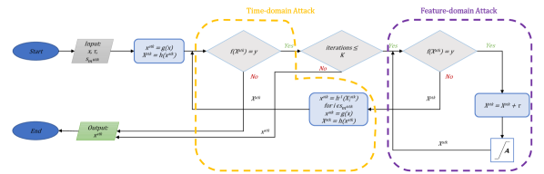
Figure 1: Attack algorithm flowchart showing the integration of time-domain attacks and feature-domain attacks to generate PMU attacks.

III-A Targeted Adversarial Example Generation

Algorithm 1 (illustrated in Fig. 1) describes how we generate adversarial PMU data. The algorithm utilizes the knowledge of classification models to perturb an incoming feature vector such that the direction of the perturbation is chosen to point towards the negative gradient of the classifier. The tampered vector of features is then reconstructed to obtain a time domain signal for each of the PMUs tampered by the attacker which then replace the original measurements at these PMUs. The resulting collated tampered and untampered event data across all PMUs is passed through the learned classifier for reclassification. This entire procedure is repeated until the classifier fails to classify correctly or when a maximum number of iterations $K$ is reached.

We explain the steps of Algorithm 1 as follows. The function $h$ represents the the transform function described in Section II-A, and $f$ is the classification model used by the attacker (in the white box setting, this is the same as that at the control center; in the gray box setting, it is different). First, we check whether $f(h(x))=y$; that is, whether the event is classified correctly. If not, there is no need to attack it. Next, we start with the untampered time domain data $x$ and boost it so that the PMUs controlled by the adversary are present in the feature vector; this step is represented by the function $g$, which outputs the initial time domain attack vector $x^{\text{atk}}$. In particular, recall from Section II-A that only for the $M^{\prime}$ PMUs with highest energy are the modal residues kept in the feature vector $X$. To ensure that the PMUs controlled by the attacker, denoted by the set $\mathcal{S}^{M_{\text{atk}}}$, are among these $M^{\prime}$ PMUs, their energy is boosted by applying $x^{\text{atk}}_{i}\leftarrow\lambda x^{\text{atk}}_{i}$ iteratively for all $i\in\mathcal{S}^{M_{\text{atk}}}$, where $\lambda>1$, until the set $\mathcal{S}^{M_{\text{atk}}}$ is included in the set of $M^{\prime}$ PMUs kept in the feature vector.

The perturbation vector $\tau$, which is designed based on the classification model $f$ and is meant to be a vector such that changing the feature vector in the direction of $\tau$ will cause the event to be misclassified. The precise details of designing $\tau$ are described in the next subsection. The feature vector $X^{\text{atk}}$ is extracted from $x^{\text{atk}}$ and perturbed by $\tau$ until $f(X^{\text{atk}})=y^{\prime}$ where $y^{\prime}$ is the incorrect event class label. To ensure that the tampered signal remains within reasonable bounds, the feature classes are restricted to lie within a feasible set $\mathcal{A}$, defined as

$$\mathcal{A} =\{X:|\omega_{k}^{c}|\leq\upsilon_{\omega},\ \sigma_{k}^{c}\geq\upsilon_{\sigma},\ \upsilon_{|R|,min}\leq|R_{k,i}^{c}|\leq\upsilon_{|R|,max},$$

$$\qquad\text{for all }k,c,i\}.$$ (6)

where $\upsilon_{\omega}$, $\upsilon_{\sigma}$, and $\upsilon_{|R|,min}$ and $\upsilon_{|R|,max}$ are the bounds for frequency mode, damping mode, and residual amplitude features. Note that $\theta$ is not restricted since any numerical value of it will be equivalent to a value in $[-\pi,\pi]$ when performing the modal analysis transformation but allows a larger set of feasible and relevant attacks. After perturbing $X^{\text{atk}}$ by $\tau$, it is projected onto $\mathcal{A}$ to ensure it is feasible.

Once the event features are misclassified in the inner loop, the time domain signals for the compromised PMUs are boosted before replacing the original signal replaces the original signal. The resulting tampered time-domain signal is denoted by $x^{\text{atk}}_{i}$, where $x^{\text{atk}}_{i}\leftarrow h^{-1}(X^{\text{atk}},i)$, and $h^{-1}$ denotes the inverse of feature extraction transform that recovers the time domain signal for the $i^{\text{th}}$ PMU (given by (1) without the noise term). After reconstructing $x^{\text{atk}}_{i}$, those time-domain signals are once again boosted via function $g$. Since the feature vector is related to all PMUs, but the attacker can only control a subset, the resulting time-domain attack vector $x^{\text{atk}}$ will not exactly match the feature vector $X^{\text{atk}}$. Thus, $X^{\text{atk}}$ is recomputed using feature extraction, and the loop repeats.

III-B Designing $\tau$

We describe how to find the perturbation vector $\tau$ used to design attacks in Algorithm 1 based on the classifier $f\in\{f_{LR},f_{GB}\}$. For the LR classifier, we designate the separating hyperplane by its weight vector $w^{LR}$, as in (3). Thus, we can misclassify an event by perturbing its values towards the hyperplane. To realize this, we let $\tau=-y_{i}\,\eta\,w^{LR}$ for event $i$, where $\eta\in\mathbb{R}$ is a step size chosen sufficiently small to avoid perturbing event features too much.

For GB, recall that the classifier is composed of a sum of $d^{\prime}$ decision trees, given by (5). The $m^{\text{th}}$ decision tree $\text{dt}_{m}$ is applied to the feature $j_{m}$ and is described by its two values $v_{1m},v_{2m}$ and the threshold $\text{th}_{m}$. Define a weight vector $w^{GB}\in\mathbb{R}^{d^{\prime}}$ given by

$$w^{GB}_{m}=\begin{cases}1,&v_{2m}>v_{1m}\\ -1,&v_{2m}\leq v_{1m}.\end{cases}$$ (7)

That is, $w^{GB}_{m}$ is a crude approximation to the gradient of $\text{dt}_{m}$ (which is not actually differentiable). Now we define $\tau$ for event $i$ with class $y_{i}$ as

$$\tau=-\eta\,y_{i}\sum_{m=1}^{d^{\prime}}w^{GB}_{m}\,e_{j_{k}}$$ (8)

where $e_{j}\in\mathbb{R}^{d}$ is the $j^{\text{th}}$ standard basis vector, i.e., it is zero except for the $j^{\text{th}}$ entry which is $1$. Again $\eta$ is a small step size. For example, if $y_{i}=1$, then the goal of the attacker is to decrease the output of the GB classifier, which means decreasing features associated with trees with positive gradient, and increasing features associated with trees with negative gradient. If the same feature is used in multiple trees, then by (8), this feature will be adjusted in proportion to the gradients of those trees.

Algorithm 1 Targeted Adversarial Example Generation

Input: $x,y$: untampered PMU data and true label

$\quad\qquad f$: Classification model

$\quad\qquad h$: Feature extraction transform

$\quad\qquad g$: Signal energy boosting function

$\quad\qquad\tau$: Perturbation vector

$\quad\qquad\mathcal{A}$: Feasible feature set

$\quad\qquad\mathcal{S}^{M_{\text{atk}}}$: Set of PMUs controlled by attacker

If: $f(h(x))=y$ do

Initialize: $x^{\text{atk}}\leftarrow g(x,\mathcal{S}^{M_{\text{atk}}})$

$\quad\qquad\qquad X_{\text{atk}}\leftarrow h(x^{\text{atk}})$

while $f(X^{\text{atk}})=y$ and iterations $\leq K$ do

     while $f(X^{\text{atk}})=y$ do

         $X^{\text{atk}}\leftarrow X^{\text{atk}}+\tau$

         Project $X^{\text{atk}}$ into $\mathcal{A}$

     end while

     for all $i\in\mathcal{S}^{M_{\text{atk}}}$ do

     $\qquad x^{\text{atk}}_{i}\leftarrow h^{-1}(X^{\text{atk}},i)$

     end for

     $x^{\text{atk}}\leftarrow g(x,\mathcal{S}^{M_{\text{atk}}})$

     $X^{\text{atk}}\leftarrow h(x^{\text{atk}})$

end while

Return: $x^{\text{atk}}$

IV Numerical Results

IV-A Dataset

The synthetic South Carolina 500-bus grid, consisting of 90 generators, 466 branches, and 206 loads [13], is used to generate synthetic generation loss and load loss events. A dynamic model of the system on PSS/E is used to generate event data by running dynamic simulations for 11 seconds at a sampling rate of 30Hz. The event is applied after 1 second to ensure the system has reached steady-state. Data is collected from PMUs distributed on the largest $M=95$ generator and load buses of the network (largest in terms of net generation or load). The GL events are generated by disconnecting the largest 50 generators, one per simulation run. For each such generator, 15 different loading scenarios are considered where the overall system loading varies between 90% to 100% of the net load. This is done by varying each individual load in the system randomly within its operational limits. Through this process, we obtain a total of 750 GL events. We create the LL events in a similar manner (i.e., disconnecting the largest 75 loads, one at a time, at 10 different loading scenarios varying between 90% to 100%). Thus the complete dataset has a total of $n_{D}=1500$ event samples collected from voltage magnitude, voltage angle, and frequency channels of $M=95$ PMUs.

In order to train the ML classification models, the dataset is split into three sets: 20% testing set and training sets for LR and GB each consisting of 40% of the dataset. Each set is assured to be nearly balanced across the two classes of events.

IV-B Evaluation of Base Cases

Figure 2 shows the base case performance of both models. Note that the LR and GB classifiers are trained on their respective untampered training set and evaluated on untampered testing set. The resulting test accuracy is shown in the figure. To this end, we use receiver operating characteristic area under the curve (ROC-AUC) as the accuracy metric to evaluate the performance of the base and tampered models. The base models are able to identify unseen data with high accuracy with the GB model approaching 100% accuracy and surpassing the performance of LR.

Figure 2: Base case (untampered) performance of LR and GB classification models evaluated on the testing set.

IV-C Generation and Evaluation of Adversarial Examples

As a first step towards evaluating the white box and gray box attack algorithms, we generate the tampered events as outlined earlier. The average AUC scores are plotted in Figures 3 and 4. In short, we iterate over the original events from the testing set as input to the attack algorithms and choose the feasible set bounds as

$$\upsilon_{\omega}=2\omega_{0},\ \upsilon_{\sigma}=0,\ \upsilon_{|R|,min}=0.8|R_{0}|,\ \upsilon_{|R|,max}=2|R_{0}|$$ (9)

where $\omega_{0}$ and $|R_{0}|$ are the untampered values of those features for a given event.

To evaluate the impact of attacks on different numbers of PMUs, we choose 10 random sets $\mathcal{S}_{\text{atk}}$, each consisting of $M^{\prime}=20$ PMUs. Denote $\mathcal{S}_{M^{\text{atk}}}$ as the set consisting of the first $M^{\text{atk}}$ PMUs in $\mathcal{S}_{\text{atk}}$, where $M^{\text{atk}}$ varies from $1$ to $20$. We then evaluate the attack on $\mathcal{S}_{M^{\text{atk}}}$ for each $M^{\text{atk}}$. Figures 3 and 4 show the average AUC as a function of $M^{\text{atk}}$.

We evaluate white and gray box attacks as follows. Let $f\in\{\text{LR},\text{GB}\}$ be the classification model used in the attack algorithm, and $f^{\prime}$ be the remaining classifier. In the white box setup, $f$ is both used in the attack algorithm and as the classifier applied to the generated attack data; in the gray box setup, $f$ is used in the attack algorithm and $f^{\prime}$ is used as the classifier. In other words, we run the attack algorithm using the knowledge of both classification models (LR and GB) and evaluate the output from each case using both classifiers.

For the attack against the LR classifier, the AUC scores, as shown in Fig. 3, indicate that the attack on LR, both in white box and gray box settings, is successful in dropping the AUC scores to less than $20\%$ for most of $M^{\text{atk}}$ scenarios. We also observe that the white box attack is more successful, reducing the AUC score to almost $0$ with just 3 tampered PMUs.

For the attack against the GB classifier attack, as shown in Fig. 4, we observe stronger resistance to adversarial examples in the white box setup, with a sharp drop in AUC score with $20$ tampered PMUs. Surprisingly, the gray box attack (based on the LR model) achieves a higher success rate across most of the range of numbers of tampered PMUs. That is, the LR-based attack is more successful with both the LR classifier (Fig. 3) and the GB classifier (Fig. 4). We conjecture that this is because the LR-based attack aims to manipulate all features, whereas the GB-based attacks only alters those features associated with decision trees in the GB model.

Figure 3: AUC scores as a function of the number of tampered PMUs for white (blue curve) and gray (red curve) box attacks for the logistic regression (LR) classifier.

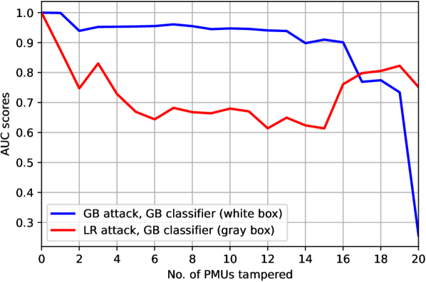
Figure 4: AUC scores as a function of the number of tampered PMUs for white (red curve) and gray (blue curve) box attacks for the gradient boosting (GB) classifier.

V Conclusion

ML-based event classification techniques can enhance situational awareness, especially with increasing DER penetration and their need for fast dynamic monitoring and response. We have introduced a framework to evaluate the robustness of such classifiers against adversarial attacks on PMU data. We have shown that sophisticated (GB) classification models are more robust to these attacks compared to simpler (LR) models. However, our findings suggest that the attack is more successful when based on the LR model, even against the GB classifier. This suggests that our white-box attack against the GB classifier can be improved, which is a subject for future work. In addition, future work will include developing classifiers to be more robust against attacks, as well as classifiers that are designed to distinguish attacks from legitimate events.

References

- [1] S. Brahma, R. Kavasseri, H. Cao, N. R. Chaudhuri, T. Alexopoulos, and Y. Cui, “Real-time identification of dynamic events in power systems using pmu data, and potential applications—models, promises, and challenges,” IEEE Transactions on Power Delivery, vol. 32, no. 1, pp. 294–301, 2017.
- [2] M. K. N. M. Sarmin, N. Saadun, M. T. Azmi, S. K. S. Abdullah, N. S. N. Yusuf, M. M. Vaiman, M. Y. Vaiman, M. Povolotskiy, and M. Karpoukhin, “Implementation of a pmu-based ems system at tnb,” in 2021 IEEE Power & Energy Society General Meeting (PESGM), 2021, pp. 1–5.
- [3] M. A. Rahman and H. Mohsenian-Rad, “False data injection attacks with incomplete information against smart power grids,” in 2012 IEEE Global Communications Conference (GLOBECOM), 2012, pp. 3153–3158.
- [4] S. Lakshminarayana, A. Kammoun, M. Debbah, and H. V. Poor, “Data-driven false data injection attacks against power grids: A random matrix approach,” IEEE Transactions on Smart Grid, vol. 12, no. 1, pp. 635–646, 2021.
- [5] A. Sayghe, O. M. Anubi, and C. Konstantinou, “Adversarial examples on power systems state estimation,” in 2020 IEEE Power & Energy Society Innovative Smart Grid Technologies Conference (ISGT), 2020, pp. 1–5.
- [6] Y. Cheng, K. Yamashita, and N. Yu, “Adversarial attacks on deep neural network-based power system event classification models,” in 2022 IEEE PES Innovative Smart Grid Technologies - Asia (ISGT Asia), 2022, pp. 66–70.
- [7] N. Taghipourbazargani, G. Dasarathy, L. Sankar, and O. Kosut, “A machine learning framework for event identification via modal analysis of pmu data,” IEEE Transactions on Power Systems, vol. 38, no. 5, pp. 4165–4176, 2023.
- [8] T. Becejac and T. Overbye, “Impact of pmu data errors on modal extraction using matrix pencil method,” in 2019 International Conference on Smart Grid Synchronized Measurements and Analytics (SGSMA), 2019, pp. 1–8.
- [9] T. Sarkar, F. hu, Y. Hua, and M. Wicks, “A real-time signal processing technique for approximating a function by a sum of complex exponentials utilizing the matrix-pencil approach,” Digital Signal Processing, vol. 4, p. 127–140, 04 1994.
- [10] K. Sheshyekani, G. Fallahi, M. Hamzeh, and M. Kheradmandi, “A general noise-resilient technique based on the matrix pencil method for the assessment of harmonics and interharmonics in power systems,” IEEE Transactions on Power Delivery, vol. 32, no. 5, pp. 2179–2188, 2017.
- [11] D. Trudnowski, J. Johnson, and J. Hauer, “Making prony analysis more accurate using multiple signals,” IEEE Transactions on Power Systems, vol. 14, no. 1, pp. 226–231, 1999.
- [12] J. H. Friedman, “Greedy function approximation: A gradient boosting machine.” The Annals of Statistics, vol. 29, no. 5, pp. 1189 – 1232, 2001. [Online]. Available: https://doi.org/10.1214/aos/1013203451
- [13] T. Xu, A. B. Birchfield, K. S. Shetye, and T. J. Overbye, “Creation of synthetic electric grid models for transient stability studies,” 2017. [Online]. Available: https://api.semanticscholar.org/CorpusID:220726884