Refining Minimax Regret for Unsupervised Environment Design

Abstract

In unsupervised environment design, reinforcement learning agents are trained on environment configurations (levels) generated by an adversary that maximises some objective. Regret is a commonly used objective that theoretically results in a minimax regret (MMR) policy with desirable robustness guarantees; in particular, the agent’s maximum regret is bounded. However, once the agent reaches this regret bound on all levels, the adversary will only sample levels where regret cannot be further reduced. Although there are possible performance improvements to be made outside of these regret-maximising levels, learning stagnates. In this work, we introduce Bayesian level-perfect MMR (BLP), a refinement of the minimax regret objective that overcomes this limitation. We formally show that solving for this objective results in a subset of MMR policies, and that BLP policies act consistently with a Perfect Bayesian policy over all levels. We further introduce an algorithm, ReMiDi, that results in a BLP policy at convergence. We empirically demonstrate that training on levels from a minimax regret adversary causes learning to prematurely stagnate, but that ReMiDi continues learning.

1 Introduction

Unsupervised environment design (UED) is an approach to automatically generate a training curriculum of environments for deep reinforcement learning (RL) agents (Dennis et al., 2020; Jiang et al., 2021a). Regret-based UED trains an adversary to select environment configurations (referred to as levels) that maximise the agent’s regret, i.e., the difference in performance between an optimal policy on that level and the agent. In other words, regret measures how much better a particular agent could perform on a particular level. Empirically, training on these regret-maximising levels has been shown to improve generalisation to out-of-distribution levels in challenging domains (Dennis et al., 2020; Jiang et al., 2021a; Parker-Holder et al., 2022; Samvelyan et al., 2023; Team et al., 2023). Furthermore, at equilibrium, UED methods theoretically result in a minimax regret policy (Dennis et al., 2020; Jiang et al., 2021a), meaning that the policy’s worst-case regret is bounded.

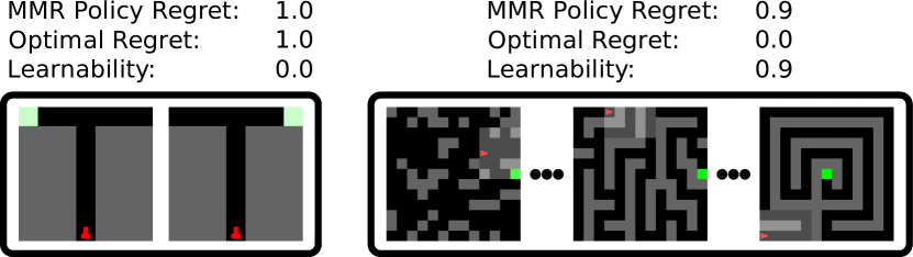
Figure 1: An illustration of the regret stagnation problem of minimax regret that our work addresses. In the T-mazes, the reward for reaching the goal is $1.0$ and $-1.0$ for failing. The reward for the mazes is $0.9$ for reaching the goal, and zero otherwise. Regret-based UED methods gravitate towards sampling high regret environments (T-mazes in this case with a regret of $1.0$), even if the agent cannot improve on these levels. This is despite the existence of non-high-regret levels (the mazes, with regret upper-bounded by $0.9$) on which the agent can still improve.

Minimax regret (MMR) works well when the agent can simultaneously perform optimally on all levels: at convergence, the MMR policy would achieve zero regret for each level. However, this is not always possible in all environments (Sukhbaatar et al., 2018). As an example, consider the T-mazes in Figure 1: these levels have different optimal behaviours but, due to partial observability, are indistinguishable to the agent. In this case, the agent cannot simultaneously perform optimally on both levels, and therefore suffers some irreducible regret. Since MMR-based UED methods prioritise sampling the highest regret levels, these two levels will continually be sampled for training—even though they provide nothing more for the agent to learn.

This phenomenon is problematic if we have a subset of levels that (a) are distinguishable from the irreducible regret levels and (b) have lower, but reducible, regret; for instance, the set of all simultaneously solvable mazes in Figure 1 (which have regret of $0.9$ or lower). A theoretically-sound UED method that implements MMR will converge to sampling each T-maze with 50% probability, and fail to sample any of the solvable mazes. While this does technically satisfy the MMR objective, there is no guarantee we will achieve a policy that is effective at solving normal mazes, as the agent would only rarely see these, if at all. This shows a weakness of MMR—which we call regret stagnation—because we know there exists a policy that obtains optimal regret on T-mazes and normal mazes.

We theoretically address this regret stagnation problem by proposing a refinement of the MMR objective, which we call Bayesian level-perfect MMR (BLP). Our objective aims to be minimax-regret over non-MMR levels, under the constraint that the policy must act according to the MMR policy in all trajectories that are consistent with MMR levels. This process is iteratively repeated, each time over a smaller subset of levels. In this way, a BLP policy retains minimax regret guarantees, and iteratively improves its worst-case regret on the remainder of the levels. We further show that any BLP policy acts consistently with a Perfect Bayesian policy on all levels. Finally, we develop an algorithm, ReMiDi, that results in a BLP policy at convergence.

Our contributions are as follows:

1. We theoretically introduce and characterise the regret stagnation problem in minimax regret UED.

2. We propose BLP, a refinement of minimax regret for UED, that retains global minimax regret, and additionally obtains minimax regret-like guarantees under trajectories that do not occur in high-regret levels.

3. We introduce a proof-of-concept algorithm, ReMiDi, that solves our new objective and returns a BLP policy.

4. We empirically demonstrate that, in settings with high irreducible regret, ReMiDi significantly outperforms standard regret-based UED.

By solving this problem, we empower the use of UED in larger and more open-ended settings, where irreducible regret is likely, as a BLP policy can be robust even outside these (potentially very rare) highest-regret levels.

2 Background

2.1 UPOMDPs

We consider an underspecified partially-observable Markov decison process (Dennis et al., 2020, UPOMDP) $\mathcal{M}=\langle A,O,\Theta,S,P_{S},P_{O},\mathcal{R},\gamma\rangle$. Here $A$ is the action space, $O$ is the observation space, and $S$ is the state space. $\Theta$ is the space of underspecified parameters commonly referred to as levels, $P_{S}:S\times A\times\Theta\to\Delta(S)$ is the level-conditional transition distribution. We denote the initial state distribution as $P_{0}:\Theta\to\Delta(S)$. In the partially observable setting, the agent does not directly observe the state, but an observation variable $o\in O$ that is correlated to the underlying state. $\mathcal{R}:S\times A\rightarrow\mathbb{R}$ is the scalar reward function, we denote instances of reward at time $t$ as $r_{t}=\mathcal{R}(s_{t},a_{t})$ and $\gamma$ is the discount factor. Each set of underspecified parameters $\theta\in\Theta$ indexes a particular POMDP called a level. In our maze example in Figure 1, the level determines the location of the goal and obstacles but dynamics such as navigating and the reward function remain shared across all levels.

At time $t$ the agent observes an action-observation history (or trajectory) $\tau_{t}=\langle o_{0},a_{0},\dots,o_{t-1},a_{t-1},o_{t}\rangle$ and chooses an action according to a trajectory-conditioned policy $a_{t}\sim\pi(\tau_{t})$. We denote the set of all trajectory-conditioned policies as $\Pi\dot{=}\{\pi|\pi:\mathcal{T}\rightarrow\Delta(A)\}$ where $\mathcal{T}$ denotes the set of all possible trajectories. For any level $\theta$, the agent’s goal is to maximise the expected discounted return (called utility), which we denote as:

$$U_{\theta}(\pi)\dot{=}\mathbb{E}_{\pi,\theta}\left[\sum_{t=0}^{T}\gamma^{t}r_{t}\right],$$

where $\mathbb{E}_{\pi,\theta}$ denotes the expected value on $\theta$ if the agent follows policy $\pi$ (Sutton & Barto, 2018). We denote an optimal policy for level $\theta$ as $\pi^{\star}_{\theta}\in\operatorname*{arg\,max}_{\pi^{\prime}}U_{\theta}(\pi^{\prime})$. Finally, similar to prior work (Dennis et al., 2020), we note that for all of the proofs in this paper we restrict our attention to finite and discrete UPOMDPs.

2.2 Unsupervised Environment Design

Unsupervised Environment Design (UED) is posed as a two-player game, where an adversary $\Lambda$ selects levels $\theta$ for an agent $\pi$ to train on (Dennis et al., 2020). The adversary’s goal is to choose levels that maximise some utility function, e.g., a constant utility for each level corresponds to domain randomisation (Tobin et al., 2017). One commonly-used objective is to maximise the agent’s regret (Savage, 1951; Bell, 1982; Loomes & Sugden, 1982). Formally, the regret of policy $\pi$ with respect to an optimal policy $\pi_{\theta}^{\star}$ on a level $\theta$ is equal to how much better $\pi_{\theta}^{\star}$ performs than $\pi$ on $\theta$, $\text{Regret}_{\theta}(\pi)\dot{=}U_{\theta}(\pi_{\theta}^{\star})-U_{\theta}(\pi)$.

If regret is used as the payoff, at equilibrium of this two-player zero-sum game, the policy satisfies minimax regret (Dennis et al., 2020):

$$\pi_{\text{MMR}}\in\Pi^{\star}_{\text{MMR}}\dot{=}\operatorname*{arg\,min}_{\pi}\{\max_{\theta\in\Theta}\{\text{Regret}_{\theta}(\pi)\}\}.$$ (1)

Constraining policies to the set of MMR policies $\Pi^{\star}_{\text{MMR}}$ has several advantages: when deploying our policy, our regret can never be higher than the minimax regret bound, so the policy has a certain degree of robustness. Using minimax regret also results in an adaptive curriculum that increases in complexity over time, leading to the agent learning more efficiently (Dennis et al., 2020; Parker-Holder et al., 2022).

Further, choosing levels based on maximising regret avoids sampling levels that are too easy (as the agent already performs well on these) or impossible (where the optimal policy also does poorly). This is in contrast to standard minimax, which tends to choose impossible levels that minimise the agent’s performance (Pinto et al., 2017; Dennis et al., 2020).

A drawback of using minimax regret is the assumption of having access to the optimal policy $\pi^{\star}_{\theta}$ per level, which is generally unavailable. To circumvent this issue, most methods approximate regret in practice. We discuss several commonly-used heuristics in Appendix C. A more serious issue with using minimax regret in isolation is that there is no formal method to choose between policies in $\Pi^{\star}_{\text{MMR}}$. Typically it is chance and initialisation that determines the policy an algorithm converges to. While all minimax regret policies protect against the highest-regret outcomes, these events may be rare and there may be significant differences in the utility of policies in $\Pi^{\star}_{\text{MMR}}$ in more commonly encountered levels. We discuss this issue further in Section 3.

3 The Limits of Minimax Regret

To elucidate the issues with using minimax regret in isolation, we analyse the set of minimax regret policies $\Pi^{\star}_{\text{MMR}}$ introduced in Section 2.2. For any $\pi_{\text{MMR}}\in\Pi^{\star}_{\text{MMR}}$ and $\vartheta\in\Theta$, it trivially holds that:

$$\operatorname{Regret}_{\vartheta}(\pi_{\text{MMR}})\leq\min_{\pi^{\prime}}\left\{\max_{\theta\in\Theta}\left\{{\operatorname{Regret}_{\theta}(\pi^{\prime})}\right\}\right\}.$$

However, it is unclear whether all policies in $\Pi^{\star}_{\text{MMR}}$ are equally desirable across all levels. In the worst case, the minimax-regret game will converge to an agent policy that only performs as well as this bound, even if further improvement is possible on other (non-minimax regret) levels. In addition, the adversary’s distribution will not change at such Nash equilibria, by definition. Thus, at equilibrium the agent will not be presented with levels outside the support of $\Lambda$ and as such will not have the opportunity to improve further—despite the possible existence of other MMR policies with lower regret outside the support of $\Lambda$.

This observation, and the concrete example in Figure 1 demonstrate that minimax regret does not always correspond to learnability: there could exist UPOMDPs with high regret on a subset of levels on which an agent is optimal (given the partial observability constraints), and low regret on levels in which it can still improve. Our key insight is that optimising solely for minimax regret can result in the agent’s learning to stop prematurely, preventing further improvement across levels outside the support of MMR levels. We summarise this regret stagnation problem of minimax regret as follows:

1. The minimax regret game is indifferent to which MMR policy is achieved on convergence; and

2. Upon convergence to a policy in $\Pi^{\star}_{\text{MMR}}$, no improvements occur on levels outside the support of $\Lambda$.

4 Refining Minimax Regret

Having described the regret stagnation problem of minimax regret, we now introduce a new objective to address it. Concretely, we propose the Bayesian level-perfect Minimax Regret (BLP) objective, our refinement of the MMR decision rule applied to UED. To describe this objective succinctly, we first introduce the notion of a realisable trajectory, and the refined MMR game. The refined game fixes a policy $\pi$ and set of levels $\Theta^{\prime}$, and restricts the solution to act consistent with $\pi$ in all trajectories possible given $\pi$ and $\Theta^{\prime}$, where behaviour for other trajectories can be chosen arbitrarily.

Definition 4.1.

(Realisable Trajectory): For a set $\Theta^{\prime}$ and policy $\pi$, $\mathcal{T}_{\pi}(\Theta^{\prime})$ denotes the set of all trajectories that are possible by following $\pi$ on any $\theta\in\Theta^{\prime}$. We call a trajectory $\tau$ realisable under $\pi$ and $\Theta^{\prime}$ iff $\tau\in\mathcal{T}_{\pi}(\Theta^{\prime})$.

Definition 4.2.

Refined Minimax Regret game: Given a UPOMDP with level space $\Theta$, suppose we have some policy $\pi$ and some subset of levels $\Theta^{\prime}\subseteq\Theta$. We introduce the refined minimax regret game under $\pi$ and $\Theta^{\prime}$, a two-player zero-sum game between an agent and adversary where:

• the agent’s strategy set is all policies of the form

  $$\pi^{\prime}(a|\tau)=\begin{cases}\pi(a|\tau)\text{ if }\tau\in\mathcal{T}_{\pi}(\Theta^{\prime})\\ \bar{\pi}(a|\tau)\text{ otherwise},\end{cases}$$

  where $\bar{\pi}$ is an arbitrary policy;

• the adversary’s strategy set is $\overline{\Theta}\dot{=}\Theta\setminus\Theta^{\prime}$;

• the adversary’s payoff is $\text{Regret}_{\theta}(\pi^{\prime})$.

In other words, $\pi^{\prime}$ represents the set of policies that perform identically to $\pi$ in any trajectory possible under $\pi$ and $\Theta^{\prime}$. At Nash equilibrium, the agent will converge to a policy that performs identically to $\pi$ under all levels in $\Theta^{\prime}$ (by definition), but otherwise will perform minimax regret optimally over $\overline{\Theta}$ with respect to these constraints. The adversary will converge onto a minimax regret equilibrium distribution with support only on levels in $\overline{\Theta}$.

We note that the solution to the refined game is not guaranteed to obtain absolute best worst-case regret over $\overline{\Theta}$, since it is constrained to act according to $\pi$ when observing certain trajectories. However, we can guarantee that the Nash solution to the refined game must obtain optimal worst-case regret compared to all other policies that also have this constraint.

We next show that the equilibrium policy of the refined game must monotonically improve upon $\pi$ in the highest-regret $\theta\in\Theta\setminus\Theta^{\prime}$, while maintaining $\pi$’s regret over $\Theta^{\prime}$.

Theorem 4.3.

Suppose we have a UPOMDP with level space $\Theta$. Let $\pi$ be some policy and $\Theta^{\prime}\subseteq\Theta$ be some subset of levels. Let $(\pi^{\prime},\Lambda^{\prime})$ denote a policy and adversary at Nash equilibrium for the refined minimax regret game under $\pi$ and $\Theta^{\prime}$. Then, (a) for all $\theta\in\Theta^{\prime}$, $\text{Regret}_{\theta}(\pi^{\prime})=\text{Regret}_{\theta}(\pi))$; and (b) we have,

$$\max_{\theta\in\Theta\setminus\Theta^{\prime}}\left\{\text{Regret}_{\theta}(\pi^{\prime})\right\}\leq\max_{\theta\in\Theta\setminus\Theta^{\prime}}\left\{\text{Regret}_{\theta}(\pi))\right\}.$$

Proof.

(a) By definition, $\pi^{\prime}$ must act according to $\pi$ on all trajectories possible under $\pi$ and $\Theta^{\prime}$. Therefore, the performance (and thus regret) of $\pi^{\prime}$ must be identical to $\pi$ for all levels in $\Theta^{\prime}$. (b) In the refined MMR game, $\pi$ is trivially in the agent’s strategy set. So regardless of what level the adversary plays, the agent can always play $\pi$. Thus the agent’s best response can never be worse than $\pi$. ∎

Theorem 4.4 next shows the benefits of iteratively refining an initial minimax regret policy.

Theorem 4.4.

(Minimax Regret Refinement Theorem):

Let $\langle\pi_{1}$, $\Lambda_{1}\rangle$ be in Nash equilibrium of the minimax regret game. Let $\langle\pi_{i},\Lambda_{i}\rangle$ with $1<i$ denote the Nash equilibrium solution to the refined minimax regret game under $\pi_{i-1}$ and $\Theta_{i}^{\prime}=\bigcup_{j=1}^{i-1}\operatorname{Supp}(\Lambda_{j})$. Then, for all $i\geq 1$, (a) $\pi_{i}$ is minimax regret and (b) we have

$$\max_{\theta\in\Theta\setminus\Theta_{i}^{\prime}}\left\{\text{Regret}_{\theta}(\pi_{i})\right\}\leq\max_{\theta\in\Theta\setminus\Theta_{i}^{\prime}}\left\{\text{Regret}_{\theta}(\pi_{i-1}))\right\}.$$ (2)

Finally, (c) for all $1\leq j<i$ and $\theta\in\text{Supp}(\Lambda_{j})$, $\text{Regret}_{\theta}(\pi_{i})=\text{Regret}_{\theta}(\pi_{j})$. In other words, iteratively refining a minimax regret policy (a) retains minimax regret guarantees; (b) monotonically improves worst-case regret on the set of levels not already sampled by any adversary; and (c) retains regret of previous refinements on previous adversaries.

Intuitively, this result holds due to inductively applying Theorem 4.3. The formal proof is in Section A.1.

We have now defined the refined game, and shown that iteratively solving it retains minimax regret guarantees and monotonically improves worst-case regret in non-MMR levels. We next describe the solution concept we propose to use instead of standard minimax regret, which we call Bayesian level-perfect Minimax Regret.

Definition 4.5.

Bayesian level-perfect Minimax Regret: Let $\langle\pi_{1},\Lambda_{1}\rangle$ be in Nash equilibrium of the minimax regret game. Let $\langle\pi_{i},\Lambda_{i}\rangle$, $1<i$ denote the solution to the refined game under $\pi_{i-1}$ and $\bigcup_{j=1}^{i-1}\operatorname{Supp}(\Lambda_{j})$.

Policy $\pi_{j}$ is a Bayesian level-perfect minimax regret policy if $\bigcup_{k=1}^{j}\operatorname{Supp}(\Lambda_{k})=\Theta$.

We refer the interested reader to Appendix B, where we discuss simpler, but ultimately flawed alternatives to BLP.

Next, Theorem 4.6 shows that BLP is similar to a Bayes perfect refinement of minimax regret, in that it acts consistently with a Perfect Bayesian policy under a minimax regret prior of levels. Its proof can be found in Section A.2.

Theorem 4.6.

A Bayesian level-perfect minimax regret policy $\pi^{\prime}$ acts consistently with a Perfect Bayesian policy on all realisable trajectories under $\pi^{\prime}$ and $\Theta$.

5 Algorithm

Having introduced our refinement of minimax regret optimality, we now introduce our proof-of-concept method Refining Minimax Regret Distributions (ReMiDi, see Algorithm 1) that learns a Bayesian level-perfect minimax regret policy. Figure 2 illustrates how our approach works.

Algorithm 1 Refining Minimax Regret Distributions

0:  Level space $\Theta$

1:  Initialise agent $\mathcal{S}=\{\}$ and adversary buffers $\mathcal{A}=\{\}$

2:  $i\leftarrow 1$

3:  while $\bigcup_{j=1}^{i}\operatorname{Supp}(\Lambda_{j})\neq\Theta$ do

4:     Initialise adversary $\Lambda_{i}$ and policy $\pi_{i}$.

5:     while $(\pi_{i},\Lambda_{i})$ is not at Nash equilibrium do

6:        Sample level $\theta\sim\Lambda_{i}$

7:        $\pi^{\prime}\leftarrow\texttt{Combine}(\mathcal{S}\cup\{\pi_{i}\},\mathcal{A})$

8:        Sample trajectory $\tau$ using $\pi^{\prime}$ and $\theta$.

9:        Let $k$ = $\max_{k}\{\tau_{k}\in\mathcal{T}_{\pi}(\bigcup_{j=1}^{i-1}\operatorname{Supp}(\Lambda_{j})))\}$

10:        if $k<|\tau|$ then

11:           Update $\pi_{i}$ and $\Lambda_{i}$ using $\theta$ and $\tau$

12:        end if

13:     end while

14:     $\mathcal{S}\leftarrow\mathcal{S}\cup\{\pi_{i}\}$

15:     $\mathcal{A}\leftarrow\mathcal{A}\cup\{\Lambda_{i}\}$

16:     $i\leftarrow i+1$

17:  end while

18:  return $\texttt{Combine}(\mathcal{S},\mathcal{A})$

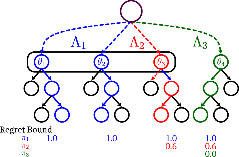
(a)

(b)

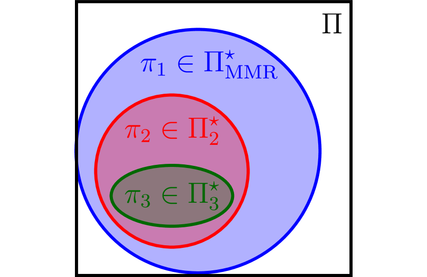
(c)

Figure 2: (a) Each node corresponds to a level-trajectory pair, and the root node indicates that the adversary samples some level $\theta$. Trajectories that are indistinguishable from each other are in the same information set, denoted by the rectangle (rectangles for singleton information sets are omitted). All nodes in the same information set are consistent with that particular trajectory. Minimax regret results in adversary ${\color[rgb]{0,0,1}\Lambda_{1}}$ and policy ${\color[rgb]{0,0,1}\pi_{1}}$, and the nodes they reach with nonzero probability are blue. Minimax regret would terminate at step 1. We instead refine our policy further. In step 2, we learn ${\color[rgb]{1,0,0}\Lambda_{2}}$ and ${\color[rgb]{1,0,0}\pi_{2}}$. The optimal policy on ${\color[rgb]{1,0,0}\theta_{3}}$ would take the dashed red line given the first observation, but our refined policy is constrained to act according to ${\color[rgb]{0,0,1}\pi_{1}}$ here. Following ${\color[rgb]{0,0,1}\pi_{1}}$ in ${\color[rgb]{1,0,0}\theta_{3}}$ leads to a trajectory that never happens under ${\color[rgb]{0,0,1}\Lambda_{1}}$ and ${\color[rgb]{0,0,1}\pi_{1}}$. In step 3, we fill in behaviour for ${\color[rgb]{0,0.40625,0}\theta_{4}}$, as these trajectories are never reached under any of the previous MMR adversaries. We terminate after all environments have been sampled by an adversary. (b) If we have a minimax regret adversary $\Lambda_{1}$, we are only guaranteed that the regret on all other levels must be at or below the regret of levels in the support of $\Lambda_{1}$ (indicated by the blue line). Refining our policy improves the bound on all levels except those sampled by $\Lambda_{1}$. We iterate this process until all levels have been sampled, monotonically improving the regret bound on all non-previously-sampled levels. (c) We illustrate that iterative refinement reduces the set of policies we consider, improving upon the initial MMR policy ${\color[rgb]{0,0,1}\pi_{1}}$.

In Algorithm 1, $\tau_{k}$ is defined as the first $k$ steps of $\tau$. $\texttt{Combine}(\mathcal{S},\mathcal{A})$ returns $\pi_{n}^{\prime}$, with $n=|\mathcal{S}|$, which is constructed as follows, with $\pi_{1}^{\prime}=\pi_{1}$ being minimax regret:

$$\pi_{n}^{\prime}(a|\tau)=\begin{cases}\pi^{\prime}_{n-1}(a|\tau)&\text{if }\tau\in\mathcal{T}_{\pi^{\prime}_{n-1}}(\bigcup_{i=1}^{n-1}\operatorname{Supp}(\Lambda_{i})))\\ \pi_{n}(a|\tau)&\text{otherwise.}\\ \end{cases}$$

Outer Loop.

Algorithm 1 is a direct implementation of the successive refined minimax regret games. Thus, at convergence, it will return a Bayesian level-perfect MMR policy. The outer loop continues until all levels have been sampled by an adversary. In practice, this is both infeasible and excessive. Thus, one may choose to only compute a fixed number of outer iterations. Lines 10-12 ensure that current adversaries only contain levels with trajectories inconsistent with the previous adversaries.

Checking for convergence in the inner loop.

Line 5 requires convergence to Nash equilibrium, which is not guaranteed to occur in practice; even if it does converge, determining when this has happened is also non-trivial. One way to approximately determine convergence is to measure the expected regret over the adversary, and if this has plateaued, we can terminate the optimisation and continue to the next level. Another, simpler technique, is to simply have a fixed number of timesteps that each adversary is trained on, and assume that (approximate) convergence is reached after training for this number of timesteps.

Choice of adversary.

Algorithm 1 is agnostic to the choice of the adversary. For instance, the adversary could be an antagonist, level generator pair (such as PAIRED (Dennis et al., 2020)), or a curated level buffer (as is used in PLR (Jiang et al., 2021b)). Note that in the case of PAIRED, only one antagonist is required for all level generators.

6 Experiments

6.1 Experimental Setup

In this section, we empirically demonstrate that the problems identified in Section 3 do occur, and that ReMiDi alleviates these issues. First, in Section 6.2, we illustrate some of the failure cases of ideal UED in a simple tabular setting. Next, in Section 6.3, we experiment in the canonical Minigrid domain. Finally, in Section 6.4, we consider a different setting where regret-based UED results in a policy that performs poorly over a large subset of levels. In each domain, we use perfect regret as our score function, i.e., the performance of the optimal policy on that level minus the performance of the agent. This is to compare against an ideal version of UED, which does not approximate regret. All plots show the mean and standard deviation over 50 (tabular experiments) or 10 (the other experiments) seeds.

For the latter experiments, we compare against Robust PLR (Jiang et al., 2021a, $\text{PLR}^{\perp}$), which is based on curating randomly-generated levels into a buffer of high-regret levels. At every step the agent is either trained on a sample of levels from the buffer, or evaluated on a set of randomly-generated levels. These randomly generated levels replace existing levels in the buffer that have lower regret scores. In robust PLR, the agent does not train on randomly generated levels. Our ReMiDi implementation maintains multiple $\text{PLR}^{\perp}$ buffers, and we perform standard $\text{PLR}^{\perp}$ on the first buffer for a certain number of iterations. We then perform $\text{PLR}^{\perp}$ again, but reject levels that have complete trajectory overlap with levels in a previous buffer. Instead of explicitly maintaining multiple policies, we have a single policy that we update only on the parts of trajectories that are distinguishable from levels in previous buffers, approximately maintaining performance on previous adversaries. Finally, Algorithm 1 assumes knowledge of whether a trajectory is possible given a policy and a set of levels, which we can compute exactly in each environment. See Appendix D for more implementation and environment details.

6.2 Exact Settings

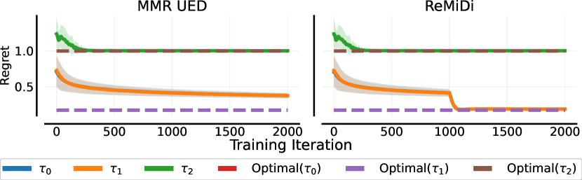
Figure 3: The greatest regret on each trajectory $\tau$ for (left) Standard Minimax Regret UED; and (right) ReMiDi. ReMiDi obtains optimal regret on all levels, whereas MMR does not.

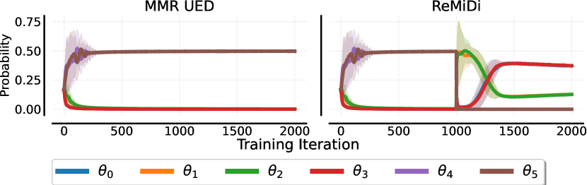
Figure 4: The Adversary’s probability of sampling each environment $\theta$ for (left) Standard Minimax Regret UED; and (b) ReMiDi. MMR UED exclusively samples the irreducible-regret levels.

We consider a one-step tabular game, where we have a set of $N$ levels $\theta_{1},\dots,\theta_{N}$. Each level $i$ corresponds to a particular initial observation $\tau_{i}$, such that the same observation may be shared by two different environments. Each level also has an associated reward for each action $a_{j},1\leq j\leq M$.

We model the adversary as a $N$-arm bandit, implemented using tabular Actor-Critic (Sutton & Barto, 2018). Each of its actions corresponds to a different level $\theta_{i}$. In our ReMiDi implementation, we have a sequence of adversaries, each selecting levels where the observations are disjoint with any previous adversary. In both cases, the agent is also a tabular Actor-Critic policy, with different action choices for each observation (equivalent to a trajectory) $\tau$.

6.2.1 When Minimax Regret is Sufficient

In Figure 5, we first consider a case where minimax regret has none of the problems discussed in Section 3. Here, each $\theta$ has a unique initial observation $\tau$, thus the level can be deduced solely from this observation. Minimax regret succeeds and converges to the globally optimal policy. Convergence occurs because a single policy can be simultaneously optimal over the set $\Theta$, as for every observation, there is one optimal action. The MMR policy is therefore also unique.

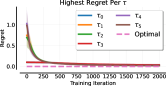
Figure 5: Plotting the regret of MMR UED throughout training for each of the $6$ trajectories. Here the optimal regret is $0$ for each trajectory, and minimax regret achieves this.

6.2.2 When Minimax Regret Fails

We next examine a UPOMDP where a single policy can no longer be simultaneously optimal over all levels. The setup is the same as the previous experiment, except that $\tau_{2}=\tau_{1}$, $\tau_{4}=\tau_{3}$, etc., meaning that there is some irreducible regret. Figure 4 shows that regret-based UED rapidly obtains minimax regret, but fails to obtain optimal regret on the non-regret-maximising levels. By contrast, ReMiDi obtains optimal regret on all levels. It does this by first obtaining global minimax regret, at which point it restricts its search over levels to those that are distinguishable from minimax regret levels. Since the agent’s policy is not updated on these prior states, it does not lose MMR guarantees.

We analyse this further in Figure 4 by plotting the probability of each level being sampled over time. Regret-based UED rapidly converges to sampling only the highest-regret levels ($\theta_{4}$ and $\theta_{5}$), and shifts the probability of sampling the other levels to zero. By contrast, our multi-step process first samples these high-regret levels exclusively. Thereafter, these are removed from the adversary’s options and it places support on all other levels. This shows that, while we could improve the performance of regret-based UED by adding stronger entropy regularisation (Mediratta et al., 2023), or making the adversary learn slower, the core limitation remains: when regret does not correspond to learnability, minimax regret UED will sample inefficiently.

6.3 Maze

We next consider Minigrid, a common benchmark in UED (Dennis et al., 2020; Jiang et al., 2021a; Parker-Holder et al., 2022). We discuss two distinct experimental settings. The first is an implementation of the T-maze example in Section 1. Here the adversary can sample T-mazes or normal mazes. The reward of T-mazes is $+1$ or $-1$ depending on whether the agent reaches the goal or not, and the standard maze reward is the same as is used in prior work (Dennis et al., 2020; Jiang et al., 2021a). The second experiment is where the adversary has the choice of blindfolding the agent; in other words, it can zero out the agent’s observation. In both cases, we evaluate on a standard set of held-out mazes.

Figure 6(a) shows that $\text{PLR}^{\perp}$ with perfect regret as its score function results in poor performance on actual mazes. The reason for this is that it almost trains exclusively on T-mazes, to the exclusion of actual mazes (see Figure 7(a)). ReMiDi, by contrast, samples T-mazes initially, and thereafter does not, as they have identical observations with previous MMR levels. This results in better performance on actual mazes.

The blindfold experiment (Figure 6(b)) shows a similar result. ReMiDi performs better than $\text{PLR}^{\perp}$; again, this is because $\text{PLR}^{\perp}$ trains the agent almost exclusively on blindfold levels (Figure 7(b)), as these have high irreducible regret. Interestingly, $\text{PLR}^{\perp}$, despite training almost exclusively on blind levels, still manages to solve many test mazes, a phenomenon investigated by Wijmans et al. (2023).

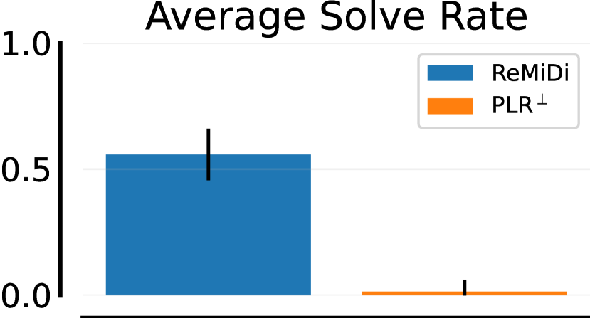
(a)

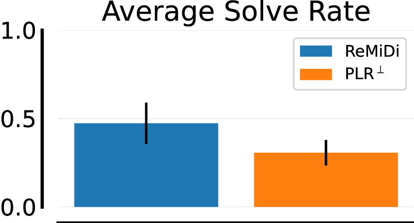
(b)

Figure 6: Solve rate on a set of held-out test mazes for the (a) T-maze and (b) blindfold experiments. ReMiDi is more effective at solving mazes than $\text{PLR}^{\perp}$.

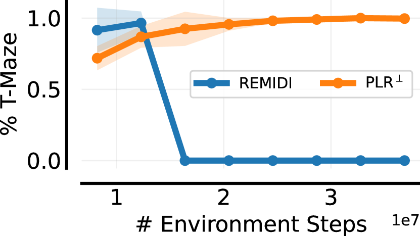
(a)

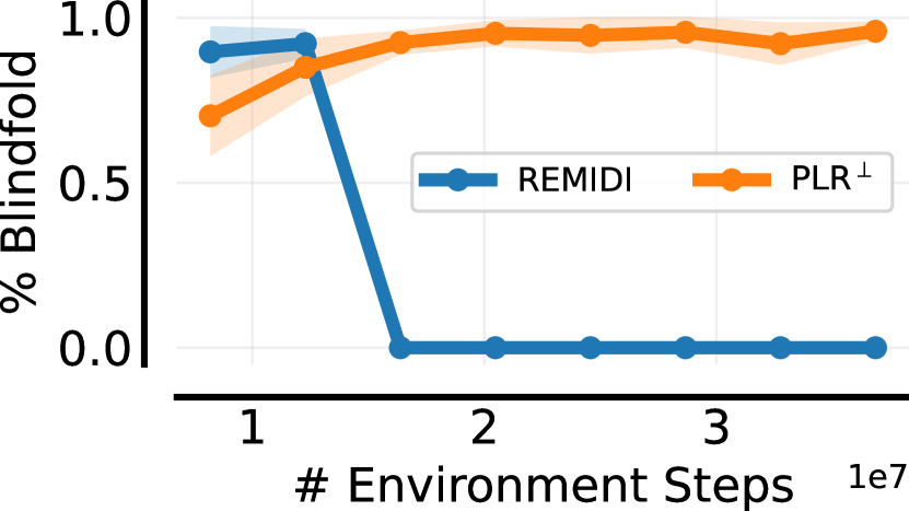
(b)

Figure 7: Fraction of replay levels that are (a) T-mazes or (b) blindfolded. $\text{PLR}^{\perp}$ converges to almost never sampling normal mazes.

6.4 Lever Game

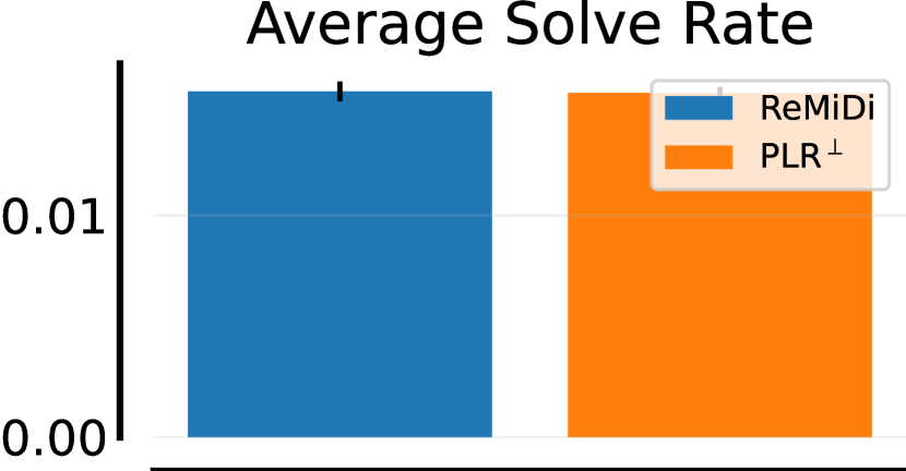
(a)

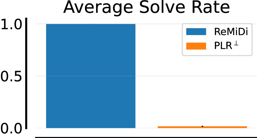
(b)

Figure 8: Solve rate in the lever game for (a) invisible; and (b) visible answers. ReMiDi can solve both types, whereas $\text{PLR}^{\perp}$ cannot, as it trained almost exclusively on invisible-answer levels.

In this environment, inspired by Hu et al. (2020), there are $64$ levers to pull, one of which is correct (reward of $+1$), and pulling a wrong lever results in a reward of $-1$. The adversary can make the correct lever known or unknown to the agent. In the latter case, the reward is multiplied by 10 (to simulate a harder problem having a higher reward). Our analysis in Section 3 suggests that regret-based UED should solely sample levels where the correct answer is unknown, and the best option for the agent is to guess randomly (as this induces irreducible regret). Training solely on these levels, however, would cause the agent to perform poorly when it observes the correct answer. Indeed, Figure 8 shows that on levels where the correct lever is not given, $\text{PLR}^{\perp}$ performs the same as ReMiDi. On levels where the correct answer is given, however, ReMiDi performs perfectly, but $\text{PLR}^{\perp}$ fails as it nearly never trained on these types of levels. Importantly, this result shows that both $\text{PLR}^{\perp}$ and ReMiDi satisfy minimax regret, but $\text{PLR}^{\perp}$ results in a policy that is effectively random, whereas ReMiDi learns a much more useful policy.

7 Related Work

Unsupervised Environment Design and Adaptive Curricula

Many recent works aim to find an adaptive curriculum for an RL agent to train on, with different methods using different metrics to choose training levels. The learning potential (Oudeyer et al., 2007) of an agent on a particular level or training example is a measure of how much an agent’s loss or reward will improve after training on this data point. Therefore, a level with a high learning potential is a promising one to train on, as the agent can still improve on it, but the level is not too difficult for the agent’s current capability. While methods based on learning potential have shown promise empirically (Florensa et al., 2018; Matiisen et al., 2020; Portelas et al., 2019), techniques that aim for robustness adversarially sample levels; for instance, adversarial minimax trains the agent in levels that minimise the agent’s performance (Pinto et al., 2017; Wang et al., 2019). However, these worst-case levels may be impossible, and therefore provide no learning benefit (Pinto et al., 2017; Dennis et al., 2020). Minimax regret provides stronger robustness guarantees (Dennis et al., 2020; Jiang et al., 2021a; Parker-Holder et al., 2022) and also alleviates the problem of minimax choosing impossible levels. Implicit in these methods is that regret corresponds to some notion of learnability (Dennis et al., 2020). However, we have shown that regret does not always coincide with learnability, and that minimax regret may cause learning to stagnate in this case, a problem ReMiDi addresses.

Decision Theory From another perspective, regret-based UED implements a minimax regret decision rule—i.e., minimising the worst-case regret (Savage, 1951; Luce & Raiffa, 1957; Peterson, 2017; Dennis et al., 2020). This decision rule provides an ordering over policies, preferring policies with lower worst-case regret. However, any two policies that have the same worst-case regret are treated as equally good by this decision rule. Our BLP objective imposes further ordering, breaking ties according to worst-case regret over all other levels that are distinguishable from MMR levels.

Game Theory and Equilibrium Refinements Our work is also related to the rich literature of Nash equilibrium refinements in game theory (Selten, 1975b, a; Kreps & Wilson, 1982; Fudenberg & Tirole, 1991; Osborne et al., 2004; Bonanno, 2015). In particular, our BLP solution concept is similar to the notion of Perfect Bayesian (or sequential) equilibria (Selten, 1975a; Fudenberg & Tirole, 1991; Kreps & Wilson, 1982), where a strategy must be optimal at all nodes of the game tree (given some belief), regardless of whether these nodes are reached under equilibrium or not.

SAMPLR Jiang et al. (2022) also focus on the limitations of standard minimax regret. They identify the problem of an automatic curriculum shifting the distribution of environment parameters away from the ground truth, which is problematic in partially-observable settings. The authors propose a solution to this problem that involves training on fictitious transitions based on the ground-truth distribution of unseen parameters. The regret stagnation problem we address—where degenerate environments with irreducible regret are continually trained on—is also a side-effect of using minimax regret in partially observable settings. Importantly, one of SAMPLR’s core assumptions is that the adversary and ground truth share support; however, as we have shown, this is not a given, as the adversary can place all of its probability mass on irreducible regret levels.

8 Discussion and Conclusion

In this work, we show that the minimax regret decision rule has a significant limitation in partially-observable settings with high irreducible regret: the minimax regret policy may perform poorly on a large subset of levels. We propose the Bayesian level-perfect objective, a refinement of minimax regret that iteratively solves smaller games, obtaining minimax regret-like performance over more environments than is guaranteed by regret-based UED, alleviating this problem of MMR. We also develop an algorithm, ReMiDi, that results in a BLP policy at convergence.

We provide theoretical justification for our approach, and show that it retains minimax regret guarantees while monotonically improving worst-case regret on non-highest-regret levels. We perform experiments in several settings with high irreducible regret and demonstrate that regret-based UED methods suffer from the regret stagnation problem we describe, causing the resulting policies to perform poorly on a large number of levels. ReMiDi, by contrast, is less susceptible to environment distributions that contain degenerate high-irreducible regret environments.

There are several promising avenues for future work, such as attempting to refine our solution concept further, to move towards true leximinimax regret (Peterson, 2017), where ties among minimax regret policies would be broken by considering the second-worst case environments, and so on (instead of considering only the second-worst case levels that are distinguishable from MMR levels). Further, we believe that the connection (and difference) between regret and learnability merits further investigation: it would be useful to disentangle the curriculum and robustness aspects of UED. It would also be promising to develop more sophisticated and efficient algorithms for obtaining BLP policies. In particular, our ReMiDi implementation requires knowing the likelihood of a trajectory under a set of environments a priori. In practice, this may not be possible or computationally feasible, and using a learned belief model could alleviate these issues (Hu et al., 2021; Jiang et al., 2022). Finally, we would like to investigate more practical ways of not degrading performance on previous adversaries, for instance, periodically training on these prior buffers.

Ultimately, we believe that UED has great potential to develop robust, generalisable and effective RL agents. Our BLP solution concept is an improved objective that obtains stronger robustness guarantees than minimax regret, and avoids its pathologies in irreducible-regret environments—paving the way for UED to be applied to more open-ended and complex task spaces.

Impact Statement

This paper presents work whose goal is to advance the field of Machine Learning. There are many potential societal consequences of our work, none which we feel must be specifically highlighted here.

Appendix A Proofs of Theoretical Results

A.1 Proof of the Minimax Regret Refinement Theorem (Theorem 4.4)

Theorem 4.4.

Let $\langle\pi_{1}$, $\Lambda_{1}\rangle$ be in Nash equilibrium of the minimax regret game. Let $\langle\pi_{i},\Lambda_{i}\rangle$ with $1<i$ denote the Nash equilibrium solution to the refined minimax regret game under $\pi_{i-1}$ and $\Theta_{i}^{\prime}=\bigcup_{j=1}^{i-1}\operatorname{Supp}(\Lambda_{j})$. Then, for all $i\geq 1$, (a) $\pi_{i}$ is minimax regret and (b) we have

$$\max_{\theta\in\Theta\setminus\Theta_{i}^{\prime}}\left\{\text{Regret}_{\theta}(\pi_{i})\right\}\leq\max_{\theta\in\Theta\setminus\Theta_{i}^{\prime}}\left\{\text{Regret}_{\theta}(\pi_{i-1}))\right\}.$$ (3)

Finally, (c) for all $1\leq j<i$ and $\theta\in\text{Supp}(\Lambda_{j})$, $\text{Regret}_{\theta}(\pi_{i})=\text{Regret}_{\theta}(\pi_{j})$.

Proof.

We first prove (a) inductively. For each $k$, we assume $\pi_{k}$ is minimax regret and must show that $\pi_{k+1}$ is also minimax regret.

Base Case: $\pi_{1}$ is trivially minimax regret by definition.

Inductive Case: Suppose $\pi_{k}$ is minimax regret. By Theorem 4.3, $\pi_{k+1}$ must have better worst-case regret than $\pi_{k}$ for the set of levels outside the support of all previous adversaries. Given this, and since $\pi_{k+1}$ is also constrained to behave identically to $\pi_{k}$ under the support of these previous adversaries, it cannot perform worse over any previously-sampled level. Thus, $\pi_{k+1}$ cannot decrease worst-case performance compared to $\pi_{k}$ on the full level set $\Theta$. Hence $\pi_{k+1}$ is minimax regret optimal.

We prove (b) inductively again.

Base Case: The case of $i=2$ follows directly from Theorem 4.3.

Inductive Case: Again, we can invoke Theorem 4.3 to show that $\pi_{i}$ must monotonically improve worst-case regret of $\pi_{i-1}$ over $\Theta\setminus\Theta^{\prime}_{i}$.

(c) This follows directly from the definition of the refined game, as $\pi_{i}$ cannot change behaviour for any level sampled by any previous adversary.

∎

A.2 Proof of Bayesian Perfect Policy (Theorem 4.6)

Theorem 4.6.

A Bayesian level-perfect minimax regret policy $\pi^{\prime}$ acts consistently with a Perfect Bayesian policy on all realisable trajectories under $\pi^{\prime}$ and $\Theta$.

Proof.

We denote $\Theta_{\tau}$ as the information set of $\tau$, consisting of all levels $\theta$ that could have generated $\tau$.

Let $\pi^{\prime}$ be a Bayesian level-perfect MMR policy (as per Definition 4.5). To show that $\pi^{\prime}$ is a Perfect Bayesian policy, we must show (a) that at every trajectory, corresponding to an information set, $\pi^{\prime}$ acts optimally with respect to some distribution $\mu(\tau)$ over $\Theta_{\tau}$. Furthermore, (b) this belief must be updated using Bayes’ rule wherever possible, i.e., we do not update the posterior on a 0 probability event.

(i): Equlibrium Paths We first consider on-equilibrium paths, i.e., those trajectories reachable by $\pi_{1}$ and $\Lambda_{1}$.

Define

$$W=\min_{\pi\in\Pi}\left\{\max_{\theta\in\Theta}\{\text{Regret}_{\theta}(\pi)\}\right\}$$

to be the optimal worst-case regret.

Since $\pi^{\prime}$ and $\Lambda_{1}$ are in equilibrium of the minimax regret game, we have that, for each $\theta\in\text{Supp}(P_{\Lambda_{1}}(\theta))$, $\text{Regret}_{\theta}(\pi^{\prime})=W$. Therefore, for any probability distribution $P^{\prime}(\theta)$ such that $\text{Supp}(P^{\prime}(\theta))\subseteq\text{Supp}(P_{\Lambda_{1}}(\theta))$, we have that

$$\mathbb{E}_{\theta\sim P^{\prime}(\theta)}[\text{Regret}_{\theta}(\pi^{\prime})]=W.$$

Now, let $\tau$ be any trajectory along the equilibrium path. Then we know that $P(\theta|\tau)$ is a probability distribution that has support that is a subset of the support of $\Lambda_{1}$.

Assume, for the sake of contradiction, that there exists a policy $\bar{\pi}$ that obtains a lower expected regret over $P(\theta|\tau)$. If this is true, it must mean that $\bar{\pi}$ improves upon $\pi^{\prime}$ in some environments in the support of $P(\theta|\tau)$. Since $\text{Supp}(P(\theta|\tau))\subseteq\text{Supp}(P_{\Lambda_{1}}(\theta))$, $\bar{\pi}$ must improve in performance compared to $\pi^{\prime}$ over the entire distribution $P_{\Lambda_{1}}(\theta)$. This provides the contradiction, since $\pi^{\prime}$ and $\Lambda_{1}$ are at Nash equilibrium—therefore, there does not exist a policy $\bar{\pi}$ that obtains a better utility while the adversary is fixed.

(ii): Off-Equilibrium Paths Let $\tau$ be a realisable trajectory that is not reached under $\Lambda_{1}$ and $\pi_{1}$. Let $i$ be the smallest integer such that $\tau$ is reached under $\Lambda_{i}$ and $\pi^{\prime}_{i}$. Then, using $\Lambda_{i}$ as the prior and performing Bayesian updating using $\pi^{\prime}_{i}$ will result in a well-defined probability distribution over $\Theta_{\tau}$. If there exists a policy that performs better starting at $\tau$ than $\pi_{i}^{\prime}$ over this distribution, then—similarly to case (i)—that contradicts $\pi_{i}^{\prime}$ being a Nash equilibrium of the $i$-th refined game. Therefore, by contradiction, $\pi^{\prime}$ satisfies (a) on off-equilibrium paths.

(iii): Non-Realisable Paths Consider a trajectory that does not occur under any $\Lambda_{i}$, $\pi^{\prime}_{i}$. This must mean that the trajectory can happen in some environment $\theta$, but $\pi^{\prime}_{i}$ never acts such that this trajectory occurs. Let $\tau$ denote one of these non-realisable trajectories. If $\pi^{\prime}$ is strictly dominated over the information set $\Theta_{\tau}$, let $\bar{\pi}$ be any policy that weakly dominates $\pi^{\prime}$ and is itself not strictly dominated. This must exist, as some strategies must survive iterated deletion of strictly-dominated strategies (Osborne & Rubinstein, 1994, Proposition 61.2).

We can modify $\pi^{\prime}$’s actions in all descendants $\tau^{\prime}$ of $\tau$ to act according to $\bar{\pi}$. We call this modified policy $\pi_{\text{bayes}}$. This policy acts according to $\pi^{\prime}$ in all realisable trajectories, and therefore obtains the same regret in all environments.

If $\pi^{\prime}$ is not strictly dominated, we can let $\pi_{\text{bayes}}$ act according to $\pi^{\prime}$ on all descendants of $\tau$.

Then, in either case, we have that $\pi_{\text{bayes}}$ is not strictly dominated over $\Theta_{\tau}$, and therefore must be optimal over some distribution $\mu(\Theta_{\tau})$ (See Lemma 60.1 of Osborne & Rubinstein (1994)).

By (i) and (ii), we have that $\pi_{\text{bayes}}$ satisfies optimality over some belief (which is updated using Bayes’ rule) on all realisable paths. By construction, we must have that $\pi_{\text{bayes}}$ also satisfies this on all non-realisable paths. Therefore, $\pi_{\text{bayes}}$ is a Perfect Bayesian policy. However, since $\pi^{\prime}$ acts consistently with $\pi_{\text{bayes}}$ over all realisable trajectories (by construction), $\pi^{\prime}$ acts consistently with some Perfect Bayesian policy on these realisable trajectories. This proves the result.

∎

Appendix B On the Temporal Inconsistency of Minimax Regret

In this section we expand upon some simpler, but ultimately flawed alternatives to our BLP formulation.

Global Regret One possible approach is to consider each trajectory $\tau$, and the associated set of levels consistent with it $\Theta_{\tau}$. We could aim to find the policy that satisfies MMR over all of these subsets. In other words, a policy in the intersection of $\Pi^{\star}_{\text{MMR}}$ for all $\Theta_{\tau}$:

$$\pi\in\Pi_{\mathcal{T}}\dot{=}\bigcap_{\tau\in\mathcal{T}}\operatorname*{arg\,min}_{\pi\in\Pi}\left\{\max_{\theta\in\Theta_{\tau}}\{\text{Regret}_{\theta}(\pi)\}\right\}.$$ (4)

However, a simple counterexample suffices to show that this set is not guaranteed to be non-empty in general. Consider a two-step MDP that has a single initial observation but multiple levels $\theta_{1}$ and $\theta_{2}$, each having a unique second observation $\tau_{1}$ or $\tau_{2}$, respectively. Finally, suppose that $\theta_{1}$ and $\theta_{2}$ have different optimal actions in the initial state. Then, $\Theta_{\tau_{1}}=\{\theta_{1}\}$ and $\Theta_{\tau_{2}}=\{\theta_{2}\}$, and the minimax regret policy over $\Theta_{\tau_{1}}$ and $\Theta_{\tau_{2}}$ must perform different actions given the shared initial observation. Therefore, the set of minimax regret policies over $\Theta_{\tau_{1}}$ and $\Theta_{\tau_{2}}$ must be disjoint. This means that the policy in Equation 4 is not always guaranteed to exist.

Local Regret Next, if we use a local form of regret, where regret at a trajectory $\tau$ is defined as the performance difference between the optimal agent and the current agent, given that both are initialised to $\tau$.

We propose the following environment as a counterexample to this: A two-step MDP with two levels $\theta_{A}$ and $\theta_{B}$. These share an initial state $s_{0}$, and there are two possible next states, $s_{A}$ and $s_{B}$. There is only one allowed action in $s_{0}$, which stochastically transitions to $s_{A}$ (99% probability if the level is $\theta_{A}$, 1% probability if the level is $\theta_{B}$) or $s_{B}$ (99% probability in $\theta_{B}$ and 1% in $\theta_{A}$).

Once the agent is in either $s_{A}$ or $s_{B}$, it must bet $100 on whether it is in $\theta_{A}$ (action $a_{1}$) or $\theta_{B}$ (action $a_{2}$). If it wins the bet it gains $100, otherwise it loses the $100. Any policy can therefore be described by two actions, $i$, $j$, corresponding to the policy’s actions in $s_{A}$ and $s_{B}$ respectively. Table 2 contains the utility for each policy, and Table 2 shows the regret for each policy. We note here we consider only deterministic policies, and stochastic policies can be obtained by using a mixed strategy.

Now let us consider the minimax regret policy for the entire MDP. It is clear that the policy must perform action $a_{1}$ in $\theta_{A}$ and $a_{2}$ in $\theta_{B}$, with an overall regret of $2$. Therefore, the policy $a_{1}a_{2}$ is MMR.

Table 1: The decision matrix for this MDP.

Utility	$a_{1}a_{1}$	$a_{1}a_{2}$	$a_{2}a_{1}$	$a_{2}a_{2}$
$\theta_{A}$	$+100$	$+98$	$-98$	$-100$
$\theta_{B}$	$-100$	$+98$	$-98$	$+100$

Table 2: Regret Matrix corresponding to Table 2.

Regret	$a_{1}a_{1}$	$a_{1}a_{2}$	$a_{2}a_{1}$	$a_{2}a_{2}$
$\theta_{A}$	$0$	$2$	$198$	$200$
$\theta_{B}$	$200$	$2$	$198$	$0$

Now let us consider the game starting from $s_{A}$, with utility and regret shown in Tables 4 and 4. Here we note that the policy can be described solely by one action, that which it takes in $s_{A}$.

In this case, the game is similar to matching pennies (Osborne & Rubinstein, 1994; Bonanno, 2015) and we have that the minimax regret policy must perform action $a_{1}$ and $a_{2}$, each with 50% probability. By symmetry, the same holds for the game starting at $s_{B}$. The resulting policy that satisfies minimax regret starting from both $s_{A}$ and $s_{B}$ is to act according to $a_{1}a_{1}$ 50% of the time, and according to $a_{2}a_{2}$ 50% of the time. If we apply this policy in the original game, we can see that it obtains a worst-case regret of $100$—much higher than the global MMR policy’s worst-case regret of $2$. Therefore, being minimax regret on both $s_{A}$ and $s_{B}$ causes a policy to not be minimax regret over the entire game.

Table 3: The decision matrix for the MDP starting at $s_{A}$.

Utility	$a_{1}$	$a_{2}$
$\theta_{A}$	$+100$	$-100$
$\theta_{B}$	$-100$	$+100$

Table 4: The regret for the MDP starting at $s_{A}$.

Utility	$a_{1}$	$a_{2}$
$\theta_{A}$	$0$	$200$
$\theta_{B}$	$200$	$0$

This counterexample shows that if we aim to perform minimax regret using a local regret measure at a particular trajectory $\tau$, then we can invalidate global minimax regret guarantees.

Some Intuition An intuitive explanation for why this happens is that the global policy can hedge its risk by committing 100% to $\theta_{A}$ in state $s_{A}$ and 100% to $\theta_{B}$ in $s_{B}$; in this way it has minimax regret globally because the environment can transition to either $s_{A}$ or $s_{B}$. The local policy, by contrast, assumes it is already in $s_{A}$ or $s_{B}$, and therefore has to hedge its risk in each case.

Summary The side-effect of these counterexamples is that we cannot aim to be minimax regret given any trajectory using a local regret measure, because if we change behaviour on any future trajectory, it may cause the agent to lose minimax regret guarantees. This is why our BLP formulation only alters behaviour of trajectories that never occur under the previous adversaries and policies. This allows us to circumvent this temporal inconsistency problem.

Appendix C Regret Approximations in UED

While regret has desirable theoretical properties, it is intractable to compute in general. Therefore, UED methods have to instead approximate regret. PAIRED (Dennis et al., 2020) does this by concurrently training two agents, and using the difference in performance between these as a proxy for regret. $\text{PLR}^{\perp}$ (Jiang et al., 2021a) uses two different scoring functions, Positive Value Loss (PVL) and Maximum Monte Carlo (MaxMC). PVL approximates regret as the average of the value loss (the reward obtained minus the predicted reward) over all transitions that have positive value loss in an episode. This prioritises levels on which the agent can still improve. MaxMC approximates the optimal return on any level as the best performance the agent has ever achieved on this level.

Appendix D Experimental Details

D.1 ReMiDi Implementation Details

We implement ReMiDi on top of $\text{PLR}^{\perp}$ as our base UED algorithm. The procedure is as follows. We first run $\text{PLR}^{\perp}$ normally for $N=1000$ iterations. We then initialise a new adversary. When new levels are sampled, we perform the agent’s action on every one of the levels in the previous buffer(s). Using the observations we obtain, we determine when the current trajectory is distinguishable from a trajectory from a prior adversary. If the trajectory has complete overlap with any level in the previous buffer, we do not add it to the new one. If it has partial or no overlap, we add it to the new buffer as normal (i.e., if the level has a higher score than any existing one). We continue to initialise a new adversary after every $N$ steps. For computational reasons, we only have a fixed number of adversaries, and remain at the last one after we have iterated through all of the previous ones.

The above works since each of our environments is deterministic. In stochastic settings, one could either add the random seed to the level $\theta$, in which case the environment becomes deterministic given $\theta$. Alternatively, we can learn a belief model $P(\tau|\Lambda_{i})$ concurrently with learning $\Lambda_{i}$. Then, if $P(\tau|\Lambda_{i})$ is lower than some threshold for all previous adversaries, we can consider it as distinguishable.

Finally, we approximate Algorithm 1 in that we do not train separate policies for each adversary. However, we update $\pi$ only on parts of trajectories that are distinguishable from previous adversaries. While we could periodically train the agent on levels from previous buffers to ensure it does not forget, we opt for the simpler option.

D.2 Environment Description

D.2.1 Tabular Setting

The tabular game consists of 6 environments $\theta_{1},\dots,\theta_{6}$. In the first experiment, each of these consists of a unique trajectory $\tau_{i}$. In each state, the agent can choose between two actions, $A$ and $B$. The environment terminates after one step, with rewards given by Table 5.

Table 5: The rewards of the first tabular setting

Environment	Trajectory	Reward A	Reward B
$\theta_{1}$	$\tau_{1}$	$-0.1$	$+0.1$
$\theta_{2}$	$\tau_{2}$	$+0.7$	$-0.7$
$\theta_{3}$	$\tau_{3}$	$-0.7$	$+0.7$
$\theta_{4}$	$\tau_{4}$	$+0.1$	$-0.1$
$\theta_{5}$	$\tau_{5}$	$-1.0$	$+1.0$
$\theta_{6}$	$\tau_{6}$	$+1.0$	$-1.0$

The second experiment used the same rewards, except that $\tau_{1}=\tau_{2}$, $\tau_{3}=\tau_{4}$ and $\tau_{5}=\tau_{6}$.

In both cases, the adversary and agent were implemented using tabular actor-critic (Sutton & Barto, 2018). The procedure is similar to PAIRED (Dennis et al., 2020), except that we used perfect regret (corresponding to an antagonist that is optimal on each level and does not learn). Both the agent and adversary are effectively bandit agents, and the adversary was updated using regret as the reward, and the agent’s reward was the negative of regret. When updating the agent, its reward is computed by taking the expectation over the adversary’s distribution given the action the agent takes. Likewise, when computing the regret for updating the agent, we compute the agent’s expected return over the environment selected by the adversary. At each iteration, we perform $5$ updates of the adversary and then $5$ updates of the agent.

We use $\gamma=0.95$, entropy coefficient of $0.1$, policy learning rate of $0.01$ and value function learning rate of $1.0$.

D.2.2 T-maze & Mazes

Every time we generate a new random level in this experiment, there is a 50% chance that it is a T-maze, and it is a normal maze otherwise. The T-maze’s goal is invisible to the agent, and each T-maze looks like the levels in Figure 9. The boundaries are generated randomly. This has the effect that each T-maze in our buffer is unique, even though they play identically. The T-maze terminates once the agent moves with a reward of either $+1$ or $-1$, depending if the goal is reached or not.

Figure 9: Several Examples of T-mazes

The mazes are generated using 25 walls sampled IID, similar to prior work (Jiang et al., 2021a). We use perfect Monte Carlo regret as the score. This is computed by first finding the shortest path from the agent’s start location to the goal, and computing the number of steps that would take. The optimal return is then computed using this. The regret is then computed as the optimal return, minus the average return of the agent on this level.

Agent Architecture

The agent architecture is similar to that used by prior work (Dennis et al., 2020; Jiang et al., 2021a). In particular, it observes the $5\times 5$ window in front of and including the agent. The agent uses a $3\times 3$ convolutional layer with 16 channels to process the input image. The agent’s direction is embedded into a $5$-dimensional vector. The image embedding is concatenated to the direction embedding and processed using a $256$-feature LSTM (Hochreiter & Schmidhuber, 1997). The output of this is processed by two 32-hidden node fully-connected layers, one for the policy and one for the value estimate.

Evaluation Levels

We evaluate the agent on a set of held-out standard test mazes used in prior work (Jiang et al., 2021a; Parker-Holder et al., 2022; Jiang et al., 2023). In particular, we use SixteenRooms, SixteenRooms2, Labyrinth, LabyrinthFlipped, Labyrinth2, StandardMaze, StandardMaze2, StandardMaze3, SmallCorridor and LargeCorridor.

D.2.3 Blindfold

In the blindfold experiment, levels are generated as normal, and then have a 50% chance of being “blindfold” levels, in which case the agent’s observation is filled with zeros. The agent architecture and evaluation procedure are the same as in the T-maze case.

D.2.4 Lever Game

The lever environment is a one-step environment where there are $64$ actions the agent can take. The observation consists of a $65$-dimensional, one-hot-encoded vector. If the first dimension is active, that indicates that the correct answer is hidden. If any of the other $i$ dimensions is activated, then the correct action is $i-1$. We generate levels by first choosing a correct action and then, with 50% probability, choose whether or not the correct answer is visible or not.

The reward for the visible case is $+1$, $-1$ for the correct and the incorrect answers respectively, and $+10$, $-10$ for the invisible case.

The agent’s architecture consists of two $256$-hidden node fully-connected layers, and then the same policy and value heads used in the other experiments. For hyperparameters, we use top-k prioritisation with $k=32$, and a buffer size of $64$ for PLR, where ReMiDi has two buffers of size $32$ each.

D.3 Hyperparameter Tuning

Table 6 contains the hyperparameters we used for our experiments.

We tuned $\text{PLR}^{\perp}$’s hyperparameters by training on standard mazes and choosing the hyperparameters that obtained the best performance over the evaluation levels. We used these for the minigrid experiments, and made slight changes for the simpler lever game. We performed a grid search over entropy coefficient of $\{0.01,0.0\}$, learning rate of $\{0.001,0.0001\}$, $\lambda$ of $\{0.95,0.98\}$, temperature of $\{0.3,1.0\}$ and replay rate of $\{0.5,0.8\}$.

We used the same hyperparameters for ReMiDi, except that we have an inner buffer size of 256, and 4 outer buffers for the minigrid experiments. The inner buffer size of 256 performed better than a larger buffer of 1000 but is computationally more efficient.

Table 6: Hyperparameters

Parameter	Minigrid	Lever
PPO
Number of Updates	30000	2500
$\gamma$	0.995
$\lambda_{\text{GAE}}$	0.95
PPO number of steps	256
PPO epochs	5
PPO minibatches per epoch	1
PPO clip range	0.2
PPO # parallel environments	32
Adam learning rate	0.001
Anneal LR	yes
Adam $\epsilon$	1e-5
PPO max gradient norm	0.5
PPO value clipping	yes
return normalization	no
value loss coefficient	0.5
entropy coefficient	0.0
PLR
Replay rate, $p$	0.8	0.8
Buffer size, $K$	4000	64
Scoring function	Perfect	Perfect
Prioritisation	Rank	Top K
Temperature, $\beta$	1.0	-
$k$	-	32
Staleness coefficient	0.3	0.3
ReMiDi
Number of Adversaries	4	2
Inner Buffer Size	256	32
Number of Replays per adversary	1000	1000

References

- Bell (1982) Bell, D. E. Regret in decision making under uncertainty. Operations Research, 30(5):961–981, 1982. ISSN 0030364X, 15265463. URL http://www.jstor.org/stable/170353.
- Bonanno (2015) Bonanno, G. Game theory: Parts i and ii-with 88 solved exercises. an open access textbook. Technical report, Working Paper, 2015.
- Dennis et al. (2020) Dennis, M., Jaques, N., Vinitsky, E., Bayen, A. M., Russell, S., Critch, A., and Levine, S. Emergent complexity and zero-shot transfer via unsupervised environment design. In Advances in Neural Information Processing Systems, 2020. URL https://proceedings.neurips.cc/paper/2020/hash/985e9a46e10005356bbaf194249f6856-Abstract.html.
- Florensa et al. (2018) Florensa, C., Held, D., Geng, X., and Abbeel, P. Automatic goal generation for reinforcement learning agents. In Proceedings of the 35th International Conference on Machine Learning, ICML 2018, Stockholmsmässan, Stockholm, Sweden, July 10-15, 2018, volume 80 of Proceedings of Machine Learning Research, pp. 1514–1523. PMLR, 2018. URL http://proceedings.mlr.press/v80/florensa18a.html.
- Fudenberg & Tirole (1991) Fudenberg, D. and Tirole, J. Perfect bayesian equilibrium and sequential equilibrium. journal of Economic Theory, 53(2):236–260, 1991.
- Hochreiter & Schmidhuber (1997) Hochreiter, S. and Schmidhuber, J. Long short-term memory. Neural Comput., 9(8):1735–1780, 1997. doi: 10.1162/neco.1997.9.8.1735. URL https://doi.org/10.1162/neco.1997.9.8.1735.
- Hu et al. (2020) Hu, H., Lerer, A., Peysakhovich, A., and Foerster, J. N. ”other-play” for zero-shot coordination. In Proceedings of the 37th International Conference on Machine Learning, ICML 2020, 13-18 July 2020, Virtual Event, volume 119 of Proceedings of Machine Learning Research, pp. 4399–4410. PMLR, 2020. URL http://proceedings.mlr.press/v119/hu20a.html.
- Hu et al. (2021) Hu, H., Lerer, A., Cui, B., Pineda, L., Brown, N., and Foerster, J. N. Off-belief learning. In Proceedings of the 38th International Conference on Machine Learning, volume 139 of Proceedings of Machine Learning Research, pp. 4369–4379. PMLR, 2021. URL http://proceedings.mlr.press/v139/hu21c.html.
- Jiang et al. (2021a) Jiang, M., Dennis, M., Parker-Holder, J., Foerster, J. N., Grefenstette, E., and Rocktäschel, T. Replay-guided adversarial environment design. In Advances in Neural Information Processing Systems, pp. 1884–1897, 2021a. URL https://proceedings.neurips.cc/paper/2021/hash/0e915db6326b6fb6a3c56546980a8c93-Abstract.html.
- Jiang et al. (2021b) Jiang, M., Grefenstette, E., and Rocktäschel, T. Prioritized level replay. In Proceedings of the 38th International Conference on Machine Learning, volume 139, pp. 4940–4950. PMLR, 2021b. URL http://proceedings.mlr.press/v139/jiang21b.html.
- Jiang et al. (2022) Jiang, M., Dennis, M., Parker-Holder, J., Lupu, A., Küttler, H., Grefenstette, E., Rocktäschel, T., and Foerster, J. Grounding aleatoric uncertainty for unsupervised environment design. Advances in Neural Information Processing Systems, 35:32868–32881, 2022.
- Jiang et al. (2023) Jiang, M., Dennis, M., Grefenstette, E., and Rocktäschel, T. minimax: Efficient baselines for autocurricula in jax. In Agent Learning in Open-Endedness Workshop at NeurIPS, 2023.
- Kreps & Wilson (1982) Kreps, D. M. and Wilson, R. Sequential equilibria. Econometrica: Journal of the Econometric Society, pp. 863–894, 1982.
- Loomes & Sugden (1982) Loomes, G. and Sugden, R. Regret theory: An alternative theory of rational choice under uncertainty. The Economic Journal, 92(368):805–824, 1982. ISSN 00130133, 14680297. URL http://www.jstor.org/stable/2232669.
- Luce & Raiffa (1957) Luce, R. D. and Raiffa, H. Games and Decisions: Introduction and Critical Survey. Wiley, New York, 1957.
- Matiisen et al. (2020) Matiisen, T., Oliver, A., Cohen, T., and Schulman, J. Teacher-student curriculum learning. volume 31, pp. 3732–3740, 2020. doi: 10.1109/TNNLS.2019.2934906. URL https://doi.org/10.1109/TNNLS.2019.2934906.
- Mediratta et al. (2023) Mediratta, I., Jiang, M., Parker-Holder, J., Dennis, M., Vinitsky, E., and Rocktäschel, T. Stabilizing unsupervised environment design with a learned adversary. In Conference on Lifelong Learning Agents, pp. 270–291, 2023.
- Osborne & Rubinstein (1994) Osborne, M. J. and Rubinstein, A. A course in game theory. MIT press, 1994.
- Osborne et al. (2004) Osborne, M. J. et al. An introduction to game theory, volume 3. Oxford university press New York, 2004.
- Oudeyer et al. (2007) Oudeyer, P.-Y., Kaplan, F., and Hafner, V. V. Intrinsic motivation systems for autonomous mental development. IEEE transactions on evolutionary computation, 11(2):265–286, 2007.
- Parker-Holder et al. (2022) Parker-Holder, J., Jiang, M., Dennis, M., Samvelyan, M., Foerster, J., Grefenstette, E., and Rocktäschel, T. Evolving curricula with regret-based environment design. In Proceedings of the International Conference on Machine Learning, pp. 17473–17498. PMLR, 2022. URL https://proceedings.mlr.press/v162/parker-holder22a.html.
- Peterson (2017) Peterson, M. An introduction to decision theory. Cambridge University Press, 2017.
- Pinto et al. (2017) Pinto, L., Davidson, J., Sukthankar, R., and Gupta, A. Robust adversarial reinforcement learning. In Proceedings of the 34th International Conference on Machine Learning, volume 70 of Proceedings of Machine Learning Research, pp. 2817–2826. PMLR, 06–11 Aug 2017. URL https://proceedings.mlr.press/v70/pinto17a.html.
- Portelas et al. (2019) Portelas, R., Colas, C., Hofmann, K., and Oudeyer, P. Teacher algorithms for curriculum learning of deep RL in continuously parameterized environments. In 3rd Annual Conference on Robot Learning, CoRL 2019, Osaka, Japan, October 30 - November 1, 2019, Proceedings, volume 100 of Proceedings of Machine Learning Research, pp. 835–853. PMLR, 2019. URL http://proceedings.mlr.press/v100/portelas20a.html.
- Samvelyan et al. (2023) Samvelyan, M., Khan, A., Dennis, M., Jiang, M., Parker-Holder, J., Foerster, J. N., Raileanu, R., and Rocktäschel, T. MAESTRO: open-ended environment design for multi-agent reinforcement learning. In The Eleventh International Conference on Learning Representations, ICLR 2023, Kigali, Rwanda, May 1-5, 2023. OpenReview.net, 2023. URL https://openreview.net/pdf?id=sKWlRDzPfd7.
- Savage (1951) Savage, L. J. The theory of statistical decision. Journal of the American Statistical association, 46(253):55–67, 1951.
- Selten (1975a) Selten, R. Reexamination of the perfectness concept for equilibrium points in extensive games. International Journal of Game Theory, 4, 1975a.
- Selten (1975b) Selten, R. Spieltheoretische behandlung eines oligopolmodells mit nachfrageträgheit. Zeitschrift für die gesamte Staatswissenschaft/Journal of Institutional and Theoretical Economics, (H. 2):374–374, 1975b.
- Sukhbaatar et al. (2018) Sukhbaatar, S., Lin, Z., Kostrikov, I., Synnaeve, G., Szlam, A., and Fergus, R. Intrinsic motivation and automatic curricula via asymmetric self-play. In 6th International Conference on Learning Representations. OpenReview.net, 2018. URL https://openreview.net/forum?id=SkT5Yg-RZ.
- Sutton & Barto (2018) Sutton, R. S. and Barto, A. G. Reinforcement learning: An introduction. MIT press, 2018.
- Team et al. (2023) Team, A. A., Bauer, J., Baumli, K., Baveja, S., Behbahani, F. M. P., Bhoopchand, A., Bradley-Schmieg, N., Chang, M., Clay, N., Collister, A., Dasagi, V., Gonzalez, L., Gregor, K., Hughes, E., Kashem, S., Loks-Thompson, M., Openshaw, H., Parker-Holder, J., Pathak, S., Nieves, N. P., Rakicevic, N., Rocktäschel, T., Schroecker, Y., Sygnowski, J., Tuyls, K., York, S., Zacherl, A., and Zhang, L. Human-timescale adaptation in an open-ended task space. CoRR, abs/2301.07608, 2023. doi: 10.48550/arXiv.2301.07608. URL https://doi.org/10.48550/arXiv.2301.07608.
- Tobin et al. (2017) Tobin, J., Fong, R., Ray, A., Schneider, J., Zaremba, W., and Abbeel, P. Domain randomization for transferring deep neural networks from simulation to the real world. In International Conference on Intelligent Robots and Systems, pp. 23–30. IEEE, 2017. doi: 10.1109/IROS.2017.8202133. URL https://doi.org/10.1109/IROS.2017.8202133.
- Wang et al. (2019) Wang, R., Lehman, J., Clune, J., and Stanley, K. O. Paired Open-Ended Trailblazer (POET): Endlessly generating increasingly complex and diverse learning environments and their solutions. CoRR, abs/1901.01753, 2019. URL http://arxiv.org/abs/1901.01753.
- Wijmans et al. (2023) Wijmans, E., Savva, M., Essa, I., Lee, S., Morcos, A. S., and Batra, D. Emergence of maps in the memories of blind navigation agents. AI Matters, 9(2):8–14, 2023. doi: 10.1145/3609468.3609471. URL https://doi.org/10.1145/3609468.3609471.