End-to-end Supervised Prediction of Arbitrary-size Graphs with
Partially-Masked Fused Gromov-Wasserstein Matching

Abstract

We present a novel end-to-end deep learning-based approach for Supervised Graph Prediction (SGP). We introduce an original Optimal Transport (OT)-based loss, the Partially-Masked Fused Gromov-Wasserstein loss (PM-FGW), that allows to directly leverage graph representations such as adjacency and feature matrices. PM-FGW exhibits all the desirable properties for SGP: it is node permutation invariant, sub-differentiable and handles graphs of different sizes by comparing their padded representations as well as their masking vectors. Moreover, we present a flexible transformer-based architecture that easily adapts to different types of input data. In the experimental section, three different tasks, a novel and challenging synthetic dataset (image2graph) and two real-world tasks, image2map and fingerprint2molecule - showcase the efficiency and versatility of the approach compared to competitors.

1 Introduction

This work focuses on the problem of Supervised Graph Prediction (SGP), an instance of Structured Prediction wherein the target variable is a graph and no particular assumption is made about the input variable. Emblematic applications of SGP include knowledge graph extraction (Melnyk et al., 2022) or dependency parsing (Dozat & Manning, 2017) in natural language processing, conditional graph scene generation in computer vision (Yang et al., 2022), (Chang et al., 2021), or molecule identification in chemistry (Young et al., 2021), (Wishart, 2011), to name but a few. Moreover, close with SGP is the unsupervised task of graph generation notably motivated by de novo drug design (Bresson & Laurent, 2019; De Cao & Kipf, 2018; Tong et al., 2021).

Challenges of SGP

Graph prediction raises some specific issues related to the complexity of the output space and the absence of widely accepted and used loss functions. First, the non-Euclidean nature of the output to be predicted makes both inference and learning challenging while the size of the output space is generally extremely large. Second, the arbitrary size of the output variable to be predicted requires a model with a flexible expressive power in the output space. Third, graphs are characterized by the absence of natural or ground-truth ordering of their nodes which makes comparison and prediction difficult. This particular issue calls for a node permutation invariant distance to predict graphs. Scrutinizing the literature at the lens of these issues, we note that very different methodologies have been developed. Energy-based models (see for instance (Suhail et al., 2021)) relax the problem into the learning of an energy function of input and output, surrogate regression methods (Brouard et al., 2016a) leverage implicit output embeddings in a Hilbert space and end-to-end deep learning involving a more or less straightforward decoding step (Shit et al., 2022). In what follows, we discuss relevant literature, focusing on methods that enable end-to-end learning.

Graph prediction with node ordering

One strategy to overcome the need for a permutation invariant loss is to exploit the nature of the input data to determine a node ordering, with the consequence that application to new types of data requires similar engineering. For instance, in de novo drug generation SMILES representations (Bresson & Laurent, 2019) are generally used to determine atom ordering. In semantic parsing, the target graph is a tree that can be serialized (see (Babu et al., 2021)) while in text-to-knowledge-graph, the task is reframed into a sequence-to-sequence problem, often addressed with large autoregressive models. Finally, for road map extraction from satellite images one can leverage the spatial positions of the nodes to define a unique ordering (Belli & Kipf, 2019).

Graph prediction with node matching

Another line of research proposes to address this problem more directly by aiming to solve a graph-matching problem, i.e., finding the one-to-one correspondence between nodes of the graphs. Among approaches belonging to this category, we note methods dedicated to molecule generation (Kwon et al., 2019) where the invariant loss is based on a characterization of graphs, ad-hoc to the molecule application. While being fully differentiable their loss does not generalize to other applications. In the similar topic of graph generation (Simonovsky & Komodakis, 2018) propose a more generic definition of the similarity between graphs by considering both feature and structural matching. However, they solve the problem using a two-step approach by using first a smooth matching approximation followed by a rounding step using the Hungarian algorithm to obtain a proper one-to-one matching, which comes with a high computational cost and introduces a non-differentiable step. For graph scene generation, Relationformer (Shit et al., 2022) is based on a bipartite object matching approach solved using a Hungarian matcher (Carion et al., 2020). The main shortcoming of this approach is that it fails to take into account edge similarity information in the matching process. The same problem is encountered in (Melnyk et al., 2022). We discuss Relationformer in more detail later in the article.

Graph prediction with surrogate regression

Another approach is related to surrogate regression methods. These approaches leverage an implicit embedding of the output graphs into a Hilbert space and solve the underlying vector-valued regression problem (see for instance (Brouard et al., 2016b)). While in principle surrogate regression has not been designed for end-to-end learning, (Ciliberto et al., 2020) showed that for losses with Implicit Loss Embedding (ILE) property the solution provided by the SGP model is expressed as the barycenter of weighted template graphs. This is the case for Optimal Transport distances such as the Fused Gromov-Wasserstein distance (Vayer et al., 2020). Moreover, as FGW barycenters can be computed and differentiated (Peyré et al., 2016), the method is indeed end-to-end learning as shown in (Brogat-Motte et al., 2022). However, to compute the barycenter one has to impose its size and the issue linked to the arbitrary size is not solved. Moreover, the accuracy of the prediction heavily depends on the expressivity of the barycenter, i.e. the number of templates, incurring also a heavy cost at inference time.

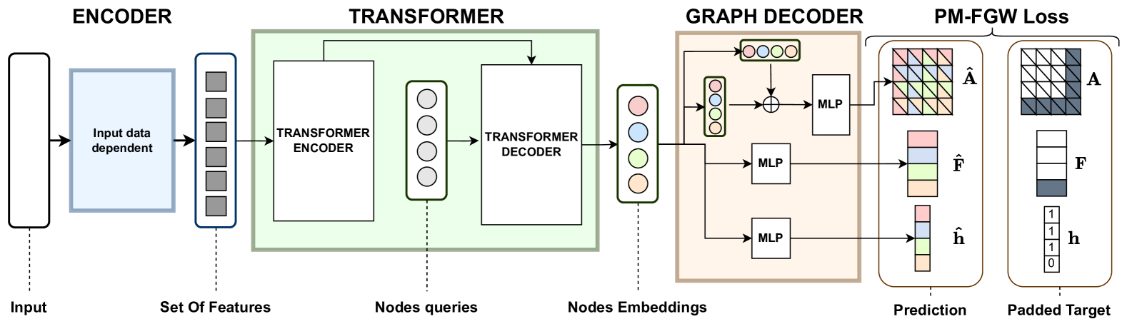
Figure 1: Illustration of the architecture for a target graph of size 3 and $M=4$.

Our contributions

The objective of this work is to propose a novel full end-to-end and versatile deep learning approach that is able to solve problems of the kind any-input2graph. To this end we introduce in Section 2 a novel loss function, that is differentiable, node permutation invariant, and able to handle graphs of varying sizes. This loss, denoted as Partially-Masked Fused Gromov-Wasserstein (PM-FGW) is a novel and necessary adaptation of the FGW distance (Vayer et al., 2020) that can be used on padded graph representation associated to a masking vector. The PM-FGW end-to-end framework is illustrated in Figure 1 and presented in Section 3 with a discussion of the optimization problem and an adaptation of deep learning architectures of (Shit et al., 2022). Finally we showcase in Section 4 the state-of-the-art performance of the proposed method, both in term of prediction accuracy and computational efficiency, on one simulated and two real world problem with different input modalities.

2 Optimal transport loss for graph prediction with arbitrary size

Hereafter, we define graph notations and provide a reminder about the FGW distance. We then propose a novel loss function that adapts FGW to enable end-to-end SGP.

2.1 Structured prediction and optimal transport

Graph notations

Let us first define the set of attributed graphs $\mathcal{G}$ that we consider as the output space of the supervised prediction task. An attributed graph $g$ with $m$ nodes can be represented by a tuple $(\mathbf{F},\mathbf{A})$ where $\mathbf{F}=[\mathbf{f}_{1},\dots,\mathbf{f}_{m}]^{\top}\in\mathbb{R}^{m\times d}$ encodes node features with $\mathbf{f}_{i}\in\mathbb{R}^{d}$ labeling each node indexed by $i$, $\mathbf{A}\in\mathbb{R}^{m\times m}$ is a pairwise distance matrix that describes the graph relationships between the nodes such as the adjacency matrix or the shortest path matrix. Further, we denote $\mathcal{G}_{m}$ the set of attributed graphs of $m$ nodes and $\mathcal{G}=\bigcup_{m=1}^{M}\mathcal{G}_{m}$, the set of attributed graphs of size up to $M$, where the size refers to the number of nodes in a graph.

In the following, we argue that a natural way to simultaneously satisfy all the requirements listed in the introduction is to rely on OT distances. Indeed, OT distances are permutation invariant and have been extended to attributed graph comparison with the FGW Distance (Vayer et al., 2019).

Fused Gromov-Wasserstein Distance (FGW) Let us recall that OT offers a mathematical and computational framework to measure discrepancies between probability distributions (Villani, 2009). The Gromov-Wasserstein (GW) distance (Mémoli, 2011) provides a way to compare probability distributions defined on different spaces. Interestingly, GW has been proposed in (Peyré et al., 2016) as a metric to compare graphs, where the graph itself is seen as a probability distribution on the set of nodes and a matrix encoding pairwise relations. For the case of interest, i.e. attributed graphs, we consider the FGW that not only takes into account the edge structure but also the node features in a graph. Along the paper, we assume a uniform probability distribution on nodes ($p_{i}=\frac{1}{m})$ for every graph of size $m$ and thus we omit $\mathbf{p}$). Given two graphs $g=(\mathbf{F},\mathbf{A})$ and $g^{\prime}=(\mathbf{F}^{\prime},\mathbf{A}^{\prime})$ with nodes of uniform weights, the FGW distance (Vayer et al., 2019) is defined as

$$\mathrm{FGW}_{\alpha}(g,g^{\prime}) =\min_{\mathbf{T}\in\pi(m,m^{\prime})}(1-\alpha)\sum_{i,j}T_{i,j}\ell_{F}(\mathbf{f}_{i},\mathbf{f}^{\prime}_{j})$$

$$+\alpha\sum_{i,j,k,l}T_{i,j}T_{k,l}\ell_{A}(A_{i,k},{A}^{\prime}_{j,l}),$$

where for two graphs of sizes $m$ and $m^{\prime}$ we denote by $\pi{(m,m^{\prime})}$ the set of transport plan $\mathbf{T}\in[0,1]^{m\times m^{\prime}}$ satisfying $\sum_{i}T_{i,j}=\frac{1}{{m^{\prime}}}$ and $\sum_{j}T_{i,j}=\frac{1}{m}$. FGW searches for an OT plan $\mathbf{T}$ that transports mass between nodes with similar labels (first term weighted by $(1-\alpha)$) and that have similar pairwise relationships (second term weighted by $\alpha$)).
Interestingly the FGW distance between two graphs with uniform weights and the same size can be seen as a relaxation of the Quadratic Assignment Problem (QAP) (Vayer et al., 2019) with an additional linear term. It is also related to the graph edit distance (Sanfeliu & Fu, 1983) as for a given alignment of graphs of the same size $\mathbf{T}$, the loss is the edit distance for node edit cost $\frac{1-\alpha}{m}\ell_{F}$ and edge edit cost $\frac{\alpha}{m^{2}}\ell_{A}$.
FGW seems to have all the properties we discussed previously and was proposed as a data-fitting term for graph prediction in (Brogat-Motte et al., 2022). However, this method does not address the question of the number of nodes that need to be provided at inference time, which greatly limits its usefulness in practice. Another very important difference is that the FGW barycenter is a computationally intensive operation that needs to be done for each new input of the model. In contrast, we propose a much more efficient architecture that relies on classical, very optimized deep learning layers. We discuss in more depth other limitations of FGW for our task.

Why is FGW not enough ?

The FGW distance necessitates equal total mass for both distributions, which is not satisfied in this scenario due to the potential disparity in the number of predicted nodes by the model. There are two possible approaches to deal with this issue. The first one consists of using uniform weights for all nodes, implying that a node on a larger graph will have a lower mass. As a result, the OT plan will share the mass among the nodes. However, this is not always suitable for practical applications as it could lead to a matching that will associate a node to potentially multiple others. The second approach is to use the Unbalanced FGW (Thual et al., 2022) which consists in relaxing the marginal constraints. However, the Unbalanced FGW introduces several additional regularization parameters that are difficult to tune because of the diversity of graphs in the dataset. Moreover, the relaxation on the marginal constraints leads to the creation and destruction of mass corresponding to a potentially partial transport of a node, which is not compatible with our initial graph alignment problem, where we need every node to be transported (with a high probability) to another node.
All aforementioned observations motivate the need to define an alternative to the FGW loss for SGP. In this work, we propose the Partially-Masked FGW loss that leverages a padded graph representation and define a novel distance between such representations.

2.2 A Partially-Masked FGW loss

In this section, we propose the Partially-Masked Fused Gromov-Wasserstein (PM-FGW) distance that serves as a loss in our approach. We first overcome the difficulty related to the arbitrary-size outputs by adopting a representation scheme suitable for any graph of size up to some fixed maximum size $M$. As discussed above the OT problem underlying the distance computation makes much more sense when considering graphs with the same number of nodes. For that reason, similarly to Relationformer (Shit et al., 2022), we implement a padding scheme on the training samples before matching to ensure that the distance is computed on graphs of the same size. Moreover, the novel distance includes an additional ground metric that accounts for comparing the occurrence of nodes.

Padding before matching and novel graph space

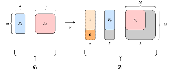
Figure 6: Illustration of the Padding operator $\mathcal{P}$ on a training example $g_{i}$. Note that after padding, the graph is of size $M$ but also associated to a padding vector $h_{i}=(1,\cdots,1,0,\cdots,0)$ that indicates which nodes are active.

The padding scheme boils down to leveraging a padding operator, denoted $\mathcal{P}$, to cast an original graph $g=(\mathbf{F}^{0},\mathbf{A}^{0})$ with $m\leq M$ nodes into a graph of size $M$. As illustrated in Figure 6 in the appendix, the transformed graph $y=\mathcal{P}(\mathbf{F}^{0},\mathbf{A}^{0})=(\mathbf{h},\mathbf{F},\mathbf{A})$ is composed of a binary multilabel masking vector $\mathbf{h}\in\{0,1\}^{M}$ that accounts for the occurrence of each node in $g$ and serves to mask the unnecessary nodes, the node feature vector $\mathbf{F}$ of size $M$ and the adjacency matrix $\mathbf{A}$ of size $M\times M$. The latter satisfy the following property: if $h_{i}=1$, then $\mathbf{f}_{i}=\mathbf{f}^{0}_{i}$, otherwise $\mathbf{f}_{i}=0$. Moreover if $h_{i}=h_{j}=1$, we have $A_{i,j}=A^{0}_{i,j}$, otherwise $A_{i,j}=0$. Equipped with this operator, we introduce $\mathcal{Y}=\mathcal{P}(\mathcal{G})$, the space of graphs padded into graphs of size $M$.

$$\mathcal{Y}=\{y=(\mathbf{h},\mathbf{F},\mathbf{A}),\mathbf{h}\in\{0,1\}^{M},\mathbf{F}\in\mathbb{R}^{M\times d},$$

$$\mathbf{A}\in\{0,1\}^{M},\exists~{}g=(\mathbf{F}^{0},\mathbf{A}^{0})\in\mathcal{G}|~{}y=\mathcal{P}g\}.$$

Further, to define properly the output space of the predictive model, we also need a relaxed version of $\mathcal{Y}$, denoted $\hat{\mathcal{Y}}$, whose elements have the following form: $\hat{y}=(\hat{\mathbf{h}},\hat{\mathbf{F}},\hat{\mathbf{A}})$ where for any $i,j\in\{1,\ldots,M\}^{2}$, $\hat{h}_{i}\in[0,1]$ and $\hat{A}_{ij}\in[0,1]$. We denote $\mathcal{T}:\hat{\mathcal{Y}}\to\mathcal{Y}$, the thresholding operator on relaxed padded graphs. For any $\hat{y}\in\hat{\mathcal{Y}}$, there exists $g\in\mathcal{G}$ such that $\mathcal{T}\hat{y}=\mathcal{P}g$.

Partially-Masked Fused Gromov-Wasserstein

The Partially-Masked Fused Gromov-Wasserstein (PM-FGW) loss between a (padded) graph $y=(\mathbf{h},\mathbf{F},\mathbf{A})\in\mathcal{Y}$ with real size $m=\|\mathbf{h}\|_{1}\leq M$ and a continuously relaxed (padded) graph $\hat{y}=(\hat{\mathbf{h}},\hat{\mathbf{F}},\hat{\mathbf{A}})$, we define $\text{PM-FGW}(y,\hat{y})$ as:

$$\min_{\mathbf{T}\in\pi(M,M)} \quad\alpha_{\text{m}}\sum_{i,i^{\prime}}T_{i,i^{\prime}}\ell_{m}(\hat{h}_{i},h_{i^{\prime}})$$ (PM-FGW)

$$+\alpha_{\text{f}}\frac{M}{m}\sum_{i,i^{\prime}}T_{i,i^{\prime}}\ell_{f}(\hat{\mathbf{f}}_{i},\mathbf{f}_{i^{\prime}})h_{i^{\prime}}$$

$$+\alpha_{\text{s}}\frac{M^{2}}{m^{2}}\sum_{i,i^{\prime},j,j^{\prime}}T_{i,i^{\prime}}T_{j,j^{\prime}}\ell_{s}(\hat{A}_{i,j},A_{i^{\prime},j^{\prime}})h_{i^{\prime}}h_{j^{\prime}},$$

where $\ell_{m}$ is a loss devoted to node mask comparison, $\ell_{f}$ to node feature comparison and $\ell_{s}$ to graph structure comparison. The normalizations in front of the sums ensure that each term is a weighted average of its internal losses as $\sum_{i,i^{\prime}}T_{i,i^{\prime}}=1$, $\sum_{i,i^{\prime}}T_{i,i^{\prime}}h_{i^{\prime}}=m/M$ and $\sum_{i,i^{\prime},j,j^{\prime}}T_{i,i^{\prime}}T_{j,j^{\prime}}h_{i^{\prime}}h_{j^{\prime}}=(m/M)^{2}$. Finally $\boldsymbol{\alpha}=[\alpha_{\text{m}},\alpha_{\text{f}},\alpha_{\text{s}}]\in\Delta_{3}$ is a triplet of hyperparameters on the simplex balancing the relative scale of $\ell_{m},\ell_{f}$ and $\ell_{A}$. For $\ell_{s}$ and $\ell_{m}$ we use the KL divergence between the predicted value after a sigmoid and the actual binary value in the target. This is equivalent to a logistic regression loss after the nodes have been matched by the OT plan. For $\ell_{f}$ we use the squared $\ell_{2}$ or the cross-entropy loss when the node features are continuous or discrete, respectively. Thus, in practice, $\ell_{A}$ and $\ell_{m}$ have the same scale and only $\alpha_{f}$ need to be carefully tuned, more details about $\boldsymbol{\alpha}$ are available in section 4.3. The global optimal transport proposed above takes simultaneously into account each property of the graphs. More precisely, the first term (node mask), ensures that the OT plan aligns together nodes that are present in the graph by matching the predicted node mask $\hat{\mathbf{h}}$ with the binary mask vector $\mathbf{h}$. This node mask ground loss enables to train the model to select properly the number of nodes. The second term (Node feature) ensures that the OT plan aligns together nodes that have close features. Finally, the last term (structure) promotes OT plans that preserve the structure of the graph by aligning together nodes that have similar pairwise relationships.

Links with other OT problem

The PM-FGW loss is an adaptation of FGW (Vayer et al., 2019) with some major changes. First, in contrast to what is usually done in OT, for each considered graph, the node masking vectors ($\mathbf{h}$ and $\mathbf{\hat{h}}$) are not used as a marginal distribution that weights the nodes but accounts for a selection of a subset of nodes. As such, when measuring the loss between two graphs, their node masking vectors are compared through the first term and only the target mask $\mathbf{h}$ is used in the second and third terms. The first term thus plays a crucial role in guiding the OT solution toward a graph with proper size. This is a key difference with FGW which is much more symmetric by design. The additional node masking term is very similar to the one of OTL_p (Thorpe et al., 2017) that proposed to use uniform marginal weight and move the part that measures the similarity between the distribution weights in an additional linear term. However, OTL_p is restricted to linear OT problems and does not use the marginal distributions as a masking for other terms as in PM-FGW. To the best of our knowledge, this is the first time that such an OT problem with partial masking has been proposed leading to a unique and simple data-fitting term when applied to SGP.
Finally, note that PM-FGW with padding is also related to Partial OT and partial GW (Chapel et al., 2020) that allows the transport of only part of the mass. Partial OT could be considered instead of padding but in this case we would discard part of the graphs and miss prediction errors with a potentially dramatic impact on the learned model.

3 Implementing End-to-end Graph Prediction with PM-FGW loss

In this section, we describe the entire end-to-end graph prediction framework we propose, starting with the optimization problem, then the proposed architecture and finally the implementation details.

3.1 PM-FGW supervised graph prediction

Wrapping up the tools introduced above we get a sound framework for graph prediction.

Empirical Risk Minimization for graph prediction

The goal of PM-FGW Supervised Graph Prediction is to learn a function $f:\mathcal{X}\to\hat{\mathcal{Y}}$ using the training samples $\{(x_{i},g_{i})\}_{i=1}^{n}\in(\mathcal{X}\times\mathcal{G})^{n}$, such that given $x$, $f$ predicts a continuously relaxed padded graph $\hat{y}:=f(x)$. Assuming $f$ is a parametric model (in this work, a deep neural network) completely determined by a generic parameter $\theta$, the supervised graph prediction writes as the following empirical risk minimization problem:

$$\min_{\theta}\quad\frac{1}{n}\sum_{i=1}^{n}\text{PM-FGW}(f_{\theta}(x_{i}),\mathcal{P}_{M}g_{i})$$

At inference time, the decoding operation boils down to passing the prediction $\hat{y}:=f_{\hat{\theta}}(x)$ through $\mathcal{T}$ then applying the inverse padding operator $\mathcal{P}^{-1}_{M}:\mathcal{Y}\to\mathcal{G}$ as follows:

$$\text{pred}(x):=\mathcal{P}^{-1}_{M}\mathcal{T}f_{\hat{\theta}}(x).$$

At training time, we work with functions whose outputs lie in $\hat{\mathcal{Y}}$, a padded and relaxed version of the original output space $\mathcal{G}$, thus avoiding a surrogate regression problem. As a result, the decoding step remains simple and inexpensive in terms of computation time.

Solving PM-FGW

Now, let’s move on to how to solve the PM-FGW problem efficiently. Our optimization problem introduced in section 2.2 is very similar to the one of FGW (Vayer et al., 2019) and can be expressed as the following quadratic problem:

$$\min_{\mathbf{T}\in\pi(M,M)}\langle\mathbf{T},\mathbf{U}\rangle+\alpha_{s}\langle\mathbf{T},\mathbf{L}\otimes\mathbf{T}\rangle$$

where $\mathbf{U}_{i,i^{\prime}}=\alpha_{m}\ell_{m}(\hat{h}_{i},h_{i^{\prime}})+\alpha_{f}\ell_{f}(\hat{\mathbf{f}}_{i},\mathbf{f}_{i^{\prime}})h_{i^{\prime}}$, $(\mathbf{L}\otimes\mathbf{T})_{i,i^{\prime}}=\sum_{j,j^{\prime}}T_{j,j^{\prime}}\ell_{s}(\hat{A}_{i,j},A_{i^{\prime},j^{\prime}})h_{i^{\prime}}h_{j^{\prime}}$ and $\langle\cdot,\cdot\rangle$ is the Frobenius scalar product. The main difference with FGW is that the tensor product encodes the partial masking of the graphs. A standard way of solving this problem (Vayer et al., 2019) is to use a conditional gradient (CG) algorithm which consists of iteratively solving a linearization of the problem. In other words at each iteration $k$ we solve a linear OT problem of cost $\langle\mathbf{T},\mathbf{C}^{(k)}\rangle$ where the linear loss $\mathbf{C}^{(k)}=\mathbf{U}+\alpha_{s}\mathbf{L}\otimes\mathbf{T}^{(k)}$ is updated at each iteration. Each step of the algorithm requires to solve a standard $\mathcal{O}(M^{3}\log M)$ OT problem, compute the tensor product $\mathbf{L}\otimes\mathbf{T}^{(k)}$ and to compute the objective value for a line search, whose overall complexity is theoretically $\mathcal{O}(M^{4})$. However, for GW and FGW, computing the tensor product (and the loss) can be accelerated to $\mathcal{O}(M^{3})$ using a matrix multiplication reformulation proposed originally in (Peyré et al., 2016). Given the non-symmetric formulation of PM-FGW and its masking part, this acceleration cannot be implemented directly. To overcome this, we propose an adapted version of this acceleration formulated below (more details are provided in appendix B).

Proposition 3.1.

The tensor product $\mathbf{L}\otimes\mathbf{T}$ and the objective value of the PM-FGW optimization problem can be computed in $\mathcal{O}(M^{3})$ by relying on matrix multiplications.

On top of this acceleration, we take advantage of two other strategies during training. First, all operations in the CG algorithm, except for linear OT solutions that use the exact solver from POT (Flamary et al., 2021), are implemented in batch parallel on GPU. This can be done thanks to the fixed size of the graphs. Second, we use a relative tolerance stopping criterion for CG which promotes early stopping. If the optimal solution isn’t achieved, we limit computational time while minimizing an upper bound on PM-FGW.

3.2 Neural network architecture

The model $f:\mathcal{X}\to\hat{\mathcal{Y}}$ (left part of Figure 1) is composed of three modules , namely the encoder that extracts features from the input, the transformer that convert these features into $M$ nodes embeddings. We expect these embeddings to capture both feature and structure information. Finally, the graph decoder that predicts the properties of our output graph, i.e., $(\hat{\mathbf{h}},\hat{\mathbf{F}},\hat{\mathbf{A}})$. Note that the proposed architecture is very much inspired by that of Relationformer (Shit et al., 2022) since the latter has been shown to lead to state-of-the-art results on many image2graph datasets. We discuss the main differences later in the section.

Encoder

The encoder extracts a number $*$ of feature vectors in $\mathbb{R}^{d_{e}}$ from the input. Note that the number of feature vectors is not fixed a priori and can depend on the input (for instance sequence length in case of text input). This is critical for encoding structures as complex as graphs and the subsequent transformer is particularly apt at treating this kind of representation. By properly designing the encoder, we can accommodate different types of input data (e.g., image, text, graph, vector). See appendix A.2 for more details.

Transformer

This module takes as input a set of feature vectors and outputs a fixed number of $M$ node embeddings. This resembles the approach taken in machine translation, and we used an architecture based on a stack of transformer encoder-decoders, akin to (Shit et al., 2022). We denote $N_{\tau}$ the number of transformer encoder/decoder layers. More details about this module are provided in appendix A.3.

Graph Decoder

This module decodes a graph from the set of node embeddings $\mathbf{Z}=[\mathbf{z}_{1},\dots,\mathbf{z}_{M}]^{T}$ using the following equation:

$$\hat{h}_{i} =\sigma(\mathrm{MLP}_{m}(\mathbf{z}_{i})) \forall i\in\{1,\dots,M\}$$

$$\hat{F}_{i} =\mathrm{MLP}_{f}(\mathbf{z}_{i}) \forall i\in\{1,\dots,M\}$$

$$\hat{A}_{i,j} =\sigma(\mathrm{MLP}_{s}(\mathbf{z}_{i}+\mathbf{z}_{j})) \forall i,j\in\{1,\dots,M\}^{2}$$

where $\sigma$ is the sigmoid function and $\mathrm{MLP}_{m}$, $\mathrm{MLP}_{f}$, $\mathrm{MLP}_{s}$ are multi-layer perceptrons heads corresponding to each component of the graph (mask, features, structure). Note that we use an operation that is symmetric in the node embeddings to compute the adjacency matrix.

Positioning with Relationformer

As discussed above, the architecture is very similar to the one proposed in Relationformer (Shit et al., 2022), with two minor changes: (1) we use a symmetric operation to compute the adjacency matrix while Relationformer uses a concatenation that is not symmetric; (2) we investigate more general encoders to enable graph prediction from data other than images. However, as stated in the previous section, the main originality of our framework lies in our PM-FGW loss. Interestingly Relationformer uses a loss that presents similarities with FGW but where the matching is done on the node features only, before computing a quadratic-linear loss similar to PM-FGW. In other words, they use a bi-level optimization problem where the plan is computed only on part of the information, which can lead to suboptimal results on heterophilic graphs.

Table 1: Graph level, edge level, and node level metrics reported on test for the different models and datasets. ^∗ denotes methods that use the actual size of the graph at inference time, hence providing a non-realistic upper-bound of their performance.

Dataset	Model	Graph Level		Edge Level		Node Level
		Edit Dist. $\downarrow$	PM-FGW $\downarrow$	Prec. $\uparrow$	Rec. $\uparrow$	Node Acc. $\uparrow$	Size Acc. $\uparrow$
Coloring	FGWBary-NN∗	7.22	0.91	71.56	80.82	84.50	n.a.
	Relationformer	5.38	0.32	78.16	84.34	99.95	99.32
	PM-FGW (ours)	0.33	0.03	98.63	98.87	99.99	99.85
Toulouse	FGWBary-NN∗	8.49	1.15	79.26	75.36	0.02	n.a.
	Relationformer	0.15	0.02	99.19	99.27	99.31	98.30
	PM-FGW (ours)	0.13	0.02	99.30	99.22	99.42	98.71
QM9	FGWBary-NN∗	6.67	1.37	80.02	64.48	79.35	n.a.
	FGWBary-ILE∗	4.10	1.27	76.49	70.67	93.48	n.a.
	Relationformer	10.17	0.49	46.62	49.07	99.60	90.79
	PM-FGW (ours)	4.02	0.28	82.91	73.51	99.72	93.41

4 Numerical experiments

Now, we present numerical experiments on simulated and real-life graph prediction problems with a comparison with state-of-the-art competitors and an in-depth analysis of the hyperparameters’ impact. The code for PM-FGW and all architectures will be released on Github.

4.1 Experimental setting

Datasets

We consider 3 different datasets that feature different modalities. First, we introduce Coloring, a new synthetic dataset inspired by the four-color theorem. The input is an image partitioned into regions of colors and the goal is to predict the graph representing the regions as nodes (4 color classes) and their connectivity in the image. Note that the outputs are complex heterophilic graphs (see Figure 2). The second dataset is Toulouse where the inputs are binarized satellite images of a city and the goal is to extract the road network (Belli & Kipf, 2019). Finally, we explore a last input modality with QM9, a small molecules dataset (Wu et al., 2018) with which we solve a set-to-graph task: from a fingerprint represented as a list of substructures (Ucak et al., 2023), the model has to predict the corresponding original molecule. The input is a list of tokens suited to our attention-based architecture. We provide examples from the datasets and additional details (e.g. size, number of nodes) in the appendix.

Compared methods

We compare our approach, referred to as PM-FGW in the following, to our direct end-to-end competitor Relationformer (Shit et al., 2022) that has shown to be the state-of-the-art method for image2graph. To have a fair comparison, we use the same architecture (presented in Figure 1) for both approaches so that the only difference is the loss. We also compare with a surrogate regression approach (FGW-Bary) based on FGW barycenters (Brogat-Motte et al., 2022) whose prediction function writes as:

$$f(x)=\operatorname*{arg\,min}_{y\in\hat{\mathcal{Y}}_{m}}\sum_{k=1}^{K}\alpha_{k}(x;W)\mathrm{FGW}_{2}^{2}(y,\bar{y}_{k}),$$ (1)

where each $\bar{y}_{k}$ denotes the $k^{th}$ template graph and $\alpha_{k}$ the $k^{th}$ weight function. We mainly use the end-to-end parametric variant, FGWBary-NN, where functions $\alpha_{k}$, as well as $K=10$ templates, are learned by a neural network. In the non-parametric variant, FGWBary-ILE, templates are training samples and $\alpha_{k}$ functions are learned by sketched kernel ridge regression (Yang et al., 2017; El Ahmad et al., 2023) and the barycenter is computed using only the $K$ largest weights to limit computational cost. However, for image processing, the parametric approach would require an ad hoc kernel based on neural network-based features. We therefore add FGWBary-ILE as a competitor only for QM9 using a Gaussian kernel on the fingerprint vectors. Finally, note that both FGWBary-NN and FGWBary-ILE cannot predict the number of nodes that needs to be artificially provided at inference time and thus, their performance can be seen as non-realistic and unfair to our method. FGWBary-NN and FGWBary-ILE have been implemented using the codes provided by Brogat-Motte et al. (2022), supplemented by specific modifications to incorporate sketching.

Performance metrics

We report several metrics to evaluate the performance of the different methods. Due to the heterogeneity of our datasets, we focus on task-agnostic metrics and evaluate several fine-grained levels of the graph. For graph level metrics we report the graph edit distance (Edit) (Gao et al., 2010) with all edit costs between the predicted graph $\mathcal{P}^{-1}_{M}\mathcal{T}\hat{y}$ and $g$ set to 1. We also report the PM-FGW distance obtained on the test data. For node and edge-level metrics, we need the graphs to have the same number of nodes. To this end, we select the $m$ nodes with the highest weight $\hat{h}_{i}$, resulting in a graph $\hat{g}=(\tilde{\mathbf{F}},\tilde{\mathbf{A}})$. This is equivalent to assuming that the size of the graph is well predicted. Then, we can compute a one-to-one matching $\sigma$ between the nodes of $\hat{g}$ and $g$ that can be used to align graphs. For edges, since we can see the adjacency matrix prediction as a classification problem we compute both the precision and recall (Prec. and Rec.) of the predicted edges with the matching. For nodes, we compute the accuracy (Node Acc.) of the node features after matching for discrete features. For Toulouse, node labels are 2D positions so we consider a prediction to be good when the l2 distance is smaller than 5% of the image width. Finally, we also report the accuracy (Size Acc.) of the predicted number of nodes for the method that predicts this property.

4.2 Comparison of SGP methods

Quantitative results

Table 1 shows the performance of the different methods on the three datasets. First, we observe that our method outperforms all competitors on Coloring which is a difficult problem that both FGWBary-NN and Relationformer struggle to solve. On Toulouse PM-FGW and Relationformer perform similarly and extremely well. This is certainly because the features (2D positions) are sufficient to uniquely identify the nodes and the structure and the LAP of Relationformer is sufficient to match the nodes. Interestingly on Toulouse, we also observe that PM-FGW converges in one iteration of CG solving the problem with the same complexity as Relationformer. Finally, on QM9, our method outperforms the other deep learning approaches on all evaluation metrics. We observe that FGWBary-ILE reaches nearly the same performance as measured by edit distance. However, this method relies on SOTA kernel and consequently suffers the heavy cost of barycenter computation. We also recall that it requires to be given the exact number of nodes at inference time.

Computational time

We report in Table 2 the ”speed” of methods both in training and inference in terms of the number of graphs processes per second. PM-FGW/Relationformer on a NVIDIA A100/Intel Xeon E5-2660 can compute at inference time 20k graphs per second on QM9 when FGWBary-NN is around 10 graphs per second because of the barycenter computation. Note that this measure does not make sense for the sketched kernel ridge regression in training as the closed-form expression is computed for all training data on CPU. Overall our proposed approach strikes the best of both worlds by achieving SOTA prediction performances at all levels of the graph, at a very low computational inference cost.

Table 2: Computational speed for the different methods in terms of graph per second on QM9.

Method	Training	Inference
FGWBary-ILE ($K$=$25$)	n.a.	1
FGWBary-NN ($K$=$10$)	10	10
Relationformer	9k	20k
PM-FGW (ours)	3k	20k

Qualitative comparison of the predicted graphs

Figure 2 shows a visual comparison of the predicted graphs for some randomly selected examples of the Coloring dataset. We observe that, in agreement with the very small observed edit distance, PM-FGW can predict perfectly most of the graphs. In contrast, Relationformer identifies well the nodes but struggles with the prediction of the structure. Finally, FGWBary-NN fails to provide a good prediction on both aspects. Additional examples from the datasets and out-of-distributions are provided in the appendix D.

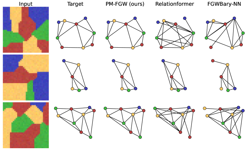
Figure 2: Predicted graphs on the Coloring dataset.

4.3 Analyzing the proposed approach

Max graph size $M$.

First, we explore the impact of $M$ on the performances of our model. We train our model on Coloring for $M$ between $10$ (default value) and $25$. To see the effective number of output nodes used by the model, we compute for all $M$ the number of nodes that are selected by the mask more than 1% of the time. Results are reported in Figure 3. Interestingly, we observe that the performances are robust w.r.t. the choice of $M$ with only a slight increase of edit distance which can be explained by the number of nodes used for prediction that reaches a plateau at $13$. This suggests that the the model automatically learns to select the correct number of nodes and one could maybe perform pruning for more efficient inference.

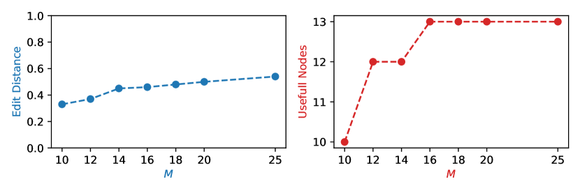
Figure 3: Effect of the parameter $M$ (maximal number of nodes) on the coloring dataset. (left) edit distance on test as a function of $M$. On the right, we plot the number of nodes out of the $M$ available that are used by the model i.e. activated at least on $1$% of the inputs.

Dataset size.

Second, we explore the impact of the size of the training set on the performances of our model. This is an important question as we leverage deep, overparameterized, neural networks. Figure 4 shows the edit distance on the test as a function of the size of the training set for all datasets. We observe that for Coloring and Toulouse the performances are stable when using the full training set, indicating that these datasets are large enough. However, for QM9 one can see that there is room for improvement when reaching the full training set (i.e. the graph edit distance is still decreasing), indicating that more data would be beneficial for this dataset. In particular, this could be beneficial to outperform FGWBary-ILE.

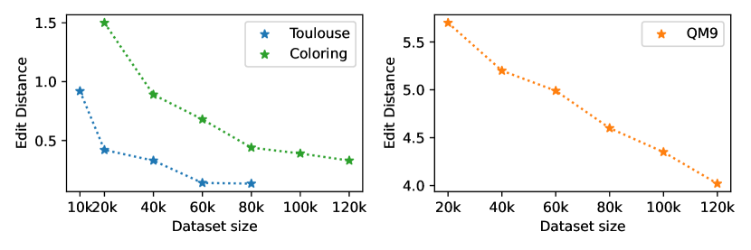
Figure 4: Performances on the test set (measured with edit distance) versus the size of the training set provided to the model.

Sensitivity to the weights $\alpha$

Finally, we investigate the impact of the weights $\alpha$ in the PM-FGW loss and study the evolution of the different terms in the loss during training. First, we train our model on Coloring for different values $\alpha$ on the simplex and report the edit distance on the test set in the left part of Figure 5. We observe that the performance is robust to the choice of $\alpha$ as long as there is not too much weight on the structure loss term (corner $\alpha_{s}=1$). The minimum error is given for $\alpha=[1/3,1/3,1/3]$ which we used in all other experiments except on Toulouse where the L2 loss needs to be scaled.
Second, we report the evolution of the three terms of the loss on the test set for uniform $\alpha$ along the epochs in the right part of Figure 5. We see that the node feature and mask terms are minimized very quickly, and then the more difficult structure term takes a longer time to decrease: probably the identification of proper nodes helps to learn the structure. This is in agreement with the behavior described above since emphasizing too much the structure term at first might lead to a local minimum that could prevent the model from learning the easier features and masks.

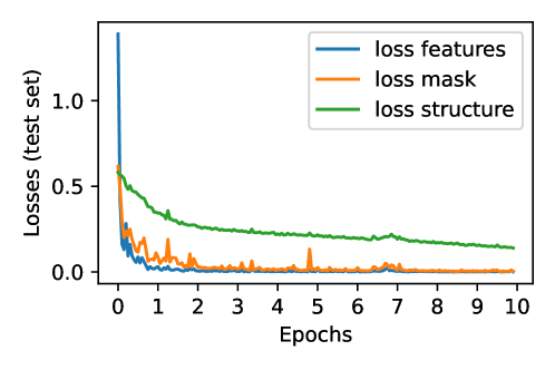
Figure 5: On the left: performances measured by edit distance for different values of $\alpha$. On the right: evolution of the three terms of the loss for the default choice $\alpha=[1/3,1/3,1/3]$, losses are evaluated on the test set every $200$ batches.

5 Conclusion

We present a novel end-to-end deep learning approach to SGP. Our approach leverages an original Optimal Transport loss based on an extension of Fused Gromov-Wasserstein that is node permutation invariant, differentiable and accounts for the difference in size between predicted and target graphs. Very good performances are obtained in different graph prediction tasks on real-world problems as well as on a new challenging synthetic task. The generality of the loss opens the door to more involved processing when comparing graph structure, e.g. exploiting spectral graph theory, a working direction that we will explore in the future together with a focus on very large datasets.

Impact Statement

This paper presents work whose goal is to advance the field of Machine Learning. There are many potential societal consequences of our work, none which we feel must be specifically highlighted here.

Appendix A Implementation details

A.1 Illustration of the padding operator

A.2 Encoder

General guidelines for the encoder.

Our framework is compatible with different types of inputs, given that one selects the appropriate encoder. The role of the encoder is to extract a set of features from the inputs $x$ i.e. each input is mapped to a list of $k$ features of dimension $d_{e}$ where $k$ is not necessarily fixed. This is critically different from extracting a unique feature vector ($k=1$) which would induce an undesirable bottleneck. To this end, we leverage convnets whenever the input is an image and transformer encoder whenever the input is a list of tokens. Other classes of encoders could be considered to address different input modalities such as Graph Neural Networks for graphs. Since the features are fed to a permutation-invariant transformer module, it is required to add a positional encoding whenever the feature representation extracted by the encoder has a meaningful ordering. Finally, we should note that the encoder might highly benefit from pre-training whenever applicable; but this goes beyond the scope of this paper.

Coloring.

In Coloring, the input is a $32\times 32\times 3$ image and the encoder consists of a CNN producing a $128\times 8\times 8$ tensor which is reshaped to $128\times(8\times 8)$ effectively outputting $64$ feature vectors. The feature vectors are then passed through a linear layer producing the desired dimension $d_{e}$. As the features are not permutation-invariant, we add spatial encoding before feeding them to the transformer module. The CNNs consist of a slight variation of Resnet18 (He et al., 2016), as we keep only the first two blocks and remove the first max-pooling layer to accommodate for the low resolution of our input image.

Toulouse.

In Toulouse, the input is a $64\times 64\times 1$ image, consequently; we use an encoder very similar to that of Coloring. Instead of removing the last two blocks of Resnet18, we remove only the last one resulting in a $256\times(8\times 8)$ output which we process as above.

QM9.

The inputs of QM9 consist of lists of $k$ tokens, where $k$ depends on the instance. Since this setting closely resembles that of natural language, we treat such inputs with a classical NLP pipeline: each token is transformed into a vector by an embedding layer and the list of vectors is then processed by a transformer encoder module. In practice, this transformer encoder and that of the encoder-decoder module are merged to avoid redundancy. Note that there is no particular ordering in the input tokens meaning that we do not need to add positional encoding as it is common practice in NLP.

A.3 Transformer encoder-decoder

General description.

The role of this module is to transform a sequence of features $\mathbf{V}=(\mathbf{v}_{1},...,\mathbf{v}_{k})$, output by the feature encoder which is not of fixed size, into a sequence of feature vectors of fixed length $M$; hence, our goal is sequence transduction. To this end we leverage the transformer encoder-decoder model  (Vaswani et al., 2017), an architecture relying on attention mechanism. First, a transformer encoder maps the input sequence of features to a sequence of representations $\mathbf{Z}=(\mathbf{z}_{1},...,\mathbf{z}_{k})$ through a self-attention mechanism :$\mathbf{Z}=T^{N_{\tau}}_{\text{Encoder}}(\mathbf{V})$. Then we use an input sequence of vectors we call node queries $\mathbf{Q}=(\mathbf{q}_{1},...,\mathbf{q}_{M})$, which are parameters of our model, as input of the decoder. Using the node queries, the decoder will attend to the encoder representation for each layer through a cross-attention mechanism. Hence the output of the model reads $T^{N_{\tau}}_{\text{Decoder}}(\mathbf{Q},\mathbf{Z})$. Please refer to section 3 of (Vaswani et al., 2017) for the details of the architecture.

Special features of our architecture

We use simple padding for the input sequence $\mathbf{V}$ as usual. As $\mathbf{Q}$ consists of parameters, there is no positional embeddings in the transformer decoder. The transformer encoder, however, may use positional embeddings depending on the type features it uses. To reduce the number of hyperparameters encoder and decoder module both consists of stacks of $N_{\tau}$ layers, with $8$ heads and the hidden dimensions of all MLP is set to $4\times d_{e}$.

A.4 Hyperparameters

We train all neural networks with the Adam optimizer, for which we decay the learning rate by a factor $10$ for the last $20$k gradient steps. All hyperparameters are given in Table 3.

Table 3: Default hyperparameters used to train our models.

Dataset	PM-FGW			Architecture			Optimization
	$\alpha_{m}$	$\alpha_{f}$	$\alpha_{s}$	$N_{\tau}$	$d_{e}$	$M$	Learning Rate	Batchsize	Training steps
Coloring	1	1	1	3	256	10	$10^{-4}$	64	100k
Toulouse	1	5	1	5	256	9	$10^{-4}$	64	100k
QM9	1	1	1	4	256	9	$10^{-4}$	32	150k

Appendix B Fast computation of the PM-FGW objective and tensor product

Proposition B.1.

Assuming that the ground loss than can decomposed as $\ell(a,b)=f_{1}(a)+f_{2}(b)-h_{1}(a)h_{2}(b)$, for any transport map $\mathbf{T}\in\pi(n,m)$ and matrices $\mathbf{A},\mathbf{W}\in\mathbb{R}^{n\times n},\mathbf{A}^{\prime},\mathbf{W}^{\prime}\in\mathbb{R}^{m\times m}$ the tensor product

$$(\mathbf{L}\otimes\mathbf{T})_{i,i^{\prime}}=\sum_{j,j^{\prime}}T_{j,j^{\prime}}\ell(A_{i,j},A_{i^{\prime},j^{\prime}}^{\prime})W_{i,j}W_{i^{\prime},j^{\prime}}^{\prime}$$

can be computed as

$$\mathbf{L}\otimes\mathbf{T} =\mathbf{U}_{1}\mathbf{T}\mathbf{W}^{\prime T}+\mathbf{W}\mathbf{T}\mathbf{U}_{2}^{T}-\mathbf{V}_{1}\mathbf{T}\mathbf{V}_{2}^{T},$$

where $\mathbf{U}_{1}=f_{1}(\mathbf{A})\cdot\mathbf{W}$, $\mathbf{U}_{2}=f_{2}(\mathbf{A}^{\prime})\cdot\mathbf{W}^{\prime}$, $\mathbf{V}_{1}=h_{1}(\mathbf{A})\cdot\mathbf{W}$, $\mathbf{V}_{2}=h_{2}(\mathbf{A}^{\prime})\cdot\mathbf{W}^{\prime}$ and $[\cdot]$ is the point-wise multiplication.

Proof.

Thanks to the decomposition assumption the tensor product can be decomposed into 3 terms:

$$(\mathbf{L}\otimes\mathbf{T})_{i,i^{\prime}} =\sum_{j,j^{\prime}}T_{j,j^{\prime}}f_{1}(A_{i,j})W_{i,j}W_{i^{\prime},j^{\prime}}^{\prime}+\sum_{j,j^{\prime}}T_{j,j^{\prime}}f_{2}(A_{i^{\prime},j^{\prime}}^{\prime})W_{i,j}W_{i^{\prime},j^{\prime}}^{\prime}-\sum_{j,j^{\prime}}T_{j,j^{\prime}}h_{1}(A_{i,j})h_{2}(A_{i^{\prime},j^{\prime}}^{\prime})W_{i,j}W_{i^{\prime},j^{\prime}}^{\prime}.$$

Rearranging the terms, we get:

$$(\mathbf{L}\otimes\mathbf{T})_{i,i^{\prime}} =\sum_{j}f_{1}(A_{i,j})W_{i,j}\sum_{j^{\prime}}T_{j,j^{\prime}}W_{i^{\prime},j^{\prime}}^{\prime}+\sum_{j^{\prime}}f_{2}(A_{i^{\prime},j^{\prime}}^{\prime})W_{i^{\prime},j^{\prime}}^{\prime}\sum_{j}T_{j,j^{\prime}}W_{i,j}-\sum_{j}h_{1}(A_{i,j})W_{i,j}\sum_{j^{\prime}}T_{j,j^{\prime}}h_{2}(A_{i^{\prime},j^{\prime}}^{\prime})W_{i^{\prime},j^{\prime}}^{\prime}.$$

Introducing $\mathbf{U}_{1},\mathbf{U}_{2},\mathbf{V}_{1}$ and $\mathbf{U}_{2}$ as defined above, we write:

$$(\mathbf{L}\otimes\mathbf{T})_{i,i^{\prime}} =\sum_{j}(U_{1})_{i,j}\sum_{j^{\prime}}T_{j,j^{\prime}}W_{i^{\prime},j^{\prime}}^{\prime}+\sum_{j^{\prime}}(U_{2})_{i^{\prime},j^{\prime}}\sum_{j}T_{j,j^{\prime}}W_{i,j}-\sum_{j}(V_{1})_{i,j}\sum_{j^{\prime}}T_{j,j^{\prime}}(V_{2})_{i^{\prime},j^{\prime}},$$

$$=\sum_{j}(U_{1})_{i,j}(TW^{\prime T})_{j,i^{\prime}}+\sum_{j^{\prime}}(U_{2})_{i^{\prime},j^{\prime}}(WT)_{i,j^{\prime}}-\sum_{j}(V_{1})_{i,j}(T_{j,j^{\prime}}V_{2}^{T})_{j,i^{\prime}},$$

which concludes that $\mathbf{L}\otimes\mathbf{T}=\mathbf{U}_{1}\mathbf{T}\mathbf{W}^{\prime T}+\mathbf{W}\mathbf{T}\mathbf{U}_{2}^{T}-\mathbf{V}_{1}\mathbf{T}\mathbf{V}_{2}^{T}$. ∎

Remark B.2 (Computational cost).

$\mathbf{U}_{1},\mathbf{U}_{2},\mathbf{V}_{1},\mathbf{V}_{2}$ can be pre-computed for a cost of $\mathcal{O}(n^{2}+m^{2})$, after which $\mathbf{L}\otimes\mathbf{T}$ can be computed (for any $\mathbf{T}$) at a cost of $\mathcal{O}(mn^{2}+nm^{2})$.

Remark B.3 (Kullback-Leibler divergence decomposition).

The Kullback-Leibler divergence $KL(p,q)=q\log\frac{q}{p}+(1-q)\log\frac{(1-q)}{(1-p)}$, which we use as ground loss in our experiments satisfies the required decomposition given $f_{1}(p)=-\log(p)$, $f_{2}(q)=q\log(q)+(1-q)\log(1-q)$, $h_{1}(p)=\log(\frac{1-p}{p})$ and, $h_{2}(q)=1-q$

Remark B.4.

The tensor product that appears in PM-FGW is a special case of this theorem that correspond to $W_{i,j}=1$ and $W^{\prime}_{i^{\prime},j^{\prime}}=h_{i^{\prime}}h_{j^{\prime}}$.

Appendix C Datasets

C.1 Overview

In this paper, we consider three datasets: Coloring, Toulouse and QM9 for which we provide a variety of statistics in Table 4. Coloring is a new synthetic dataset which we describe in detail in the next section. Similarly, a full description of Toulouse is available in (Belli & Kipf, 2019). QM9 is a dataset of small molecules commonly used for benchmarking a wide range of molecule related tasks. In our case, we compute a fingerprint of the molecule and attempt to reconstruct the original molecule from this lossy representation. Following (Ucak et al., 2023) we use the Morgan Radius-2 fingerprint which represents a molecule by a bit vector of size $2048$, where each bit represents the presence/absence of a given substructure. Finally, we feed our model with the list of non-zeros bits, i.e. the list of substructures (tokens) present in the molecule. Since the fingerprint is extremely sparse, we observe that the list of substructures has an average (respectively maximum) length of $4.5$ (respectively $23$).

Table 4: Table summarizing the properties of the datasets considered.

Dataset	Size	Nodes	Edges	Input Modality	Node features
	(train/test/valid)	(min/mean/max)	(min/mean/max)
Coloring	120k/10k/10k	4/7.0/10	3/10.9/22	Images	4 Classes (colors)
Toulouse	80k/10k/20k	3/6.1/9	2/4.9/14	Images	2D positions
QM9	120k/10k/10k	1/8.8/9	0/9.4/13	List of tokens	4 classes (atoms)

C.2 Coloring

We introduce Coloring, a new synthetic dataset well suited for benchmarking SGP methods. The main advantages of Coloring are:

• The output graph is uniquely defined from the input image.

• The complexity of the task can be finely controlled by picking the distribution of the graph sizes, the number of node labels (colors) and the resolution of the input image.

• One can generate as many pairs (inputs, output) as needed to explore different regimes, from abundant to scarce data.

To generate a new instance of Coloring, we apply the following steps:

• 0) Choose the number of nodes $m$. In this paper, we sample $m$ uniformly from $[6,10]$.

• 1) Sample $m$ centroids on $[0,1]\times[0,1]$. In this paper, we sample the centroids as uniform i.i.d. variables.

• 2) Partition $[0,1]\times[0,1]$ (the image) in a Voronoi diagram fashion (Okabe et al., 2009). In this paper, we use the $L_{1}$ distance and an image of resolution $32\times 32$.

• 3) Create the associated graph i.e. each node is a region of the image and two nodes are linked by an edge whenever the two associated regions are adjacent.

• 4) Color the graph with $K>4$ colors. In this paper, we use $K=4$. A coloring is said to be valid whenever no adjacent nodes have the same color. Note that graph coloring is known to be NP-complete (Karp, 2010).

• 5) Color the original image accordingly.

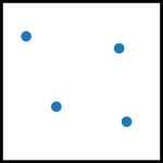
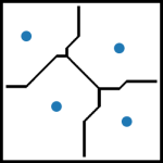
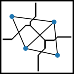
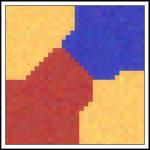
Figure 7: Illustration of the five steps to follow to generate a new instance of Coloring.

Appendix D Additional qualitative results

We present a few qualitative results to illustrate the behaviour of the PM-FGW model.

First, we tested if, once learned on Toulouse training set, the predictive model is able to cope with out-of-distribution data. Figure 8 shows that this is the case on these toy images, that are not related to satellite images or road maps. We leave for future work the investigation of this property.

Figure 8: PM-FGW Model trained on Toulouse performing on out-of-distribution inputs. Input images are displayed on top row and prediction in the bottom row.

Second, we give more examples of predicted graphs by the different methods: PM-FGW (ours), Relationformer (Shit et al., 2022), and FGWBary-NN (Brogat-Motte et al., 2022), illustrating the fact that some prediction problems are non-trivial and raise difficulty for the two competitors. Figure 9 features the Coloring prediction examples, Figure 10, those of Toulouse and Figure 11, the molecules prediction from QM9.

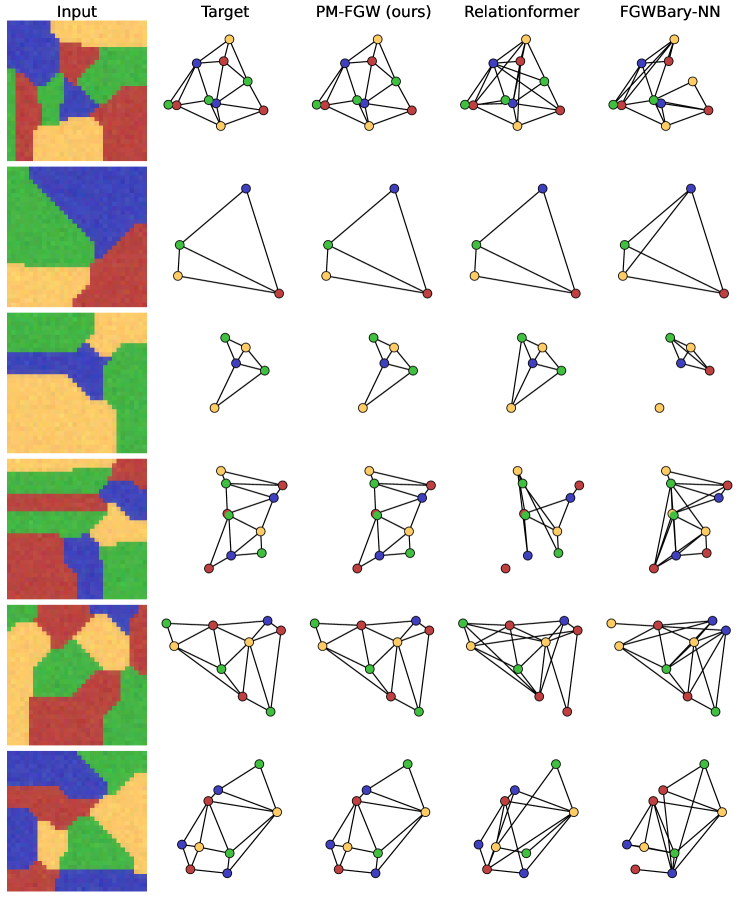
Figure 9: More predictions from the Coloring dataset.

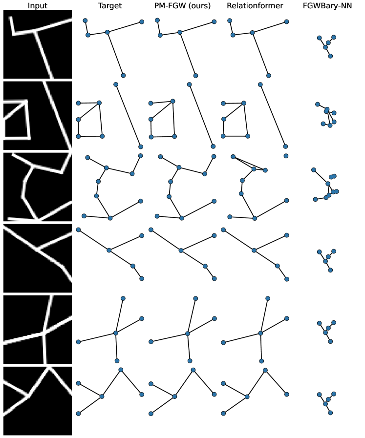
Figure 10: More predictions from the Toulouse dataset.

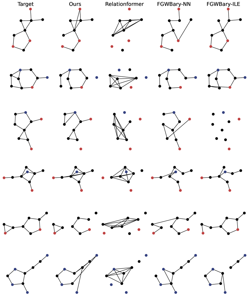
Figure 11: More predictions from the QM9 dataset. Carbon atoms are black, oxygen are red and nitrogen are blue.

References

- Babu et al. (2021) Babu, A., Shrivastava, A., Aghajanyan, A., Aly, A., Fan, A., and Ghazvininejad, M. Non-autoregressive semantic parsing for compositional task-oriented dialog. arXiv preprint arXiv:2104.04923, 2021.
- Belli & Kipf (2019) Belli, D. and Kipf, T. Image-conditioned graph generation for road network extraction. arXiv preprint arXiv:1910.14388, 2019.
- Bresson & Laurent (2019) Bresson, X. and Laurent, T. A two-step graph convolutional decoder for molecule generation. arXiv preprint arXiv:1906.03412, 2019.
- Brogat-Motte et al. (2022) Brogat-Motte, L., Flamary, R., Brouard, C., Rousu, J., and d’Alché Buc, F. Learning to predict graphs with fused gromov-wasserstein barycenters. In International Conference on Machine Learning, pp. 2321–2335. PMLR, 2022.
- Brouard et al. (2016a) Brouard, C., Shen, H., Dührkop, K., d’Alché-Buc, F., Böcker, S., and Rousu, J. Fast metabolite identification with input output kernel regression. Bioinformatics, 32(12):i28–i36, 2016a.
- Brouard et al. (2016b) Brouard, C., Szafranski, M., and d’Alché Buc, F. Input output kernel regression: Supervised and semi-supervised structured output prediction with operator-valued kernels. Journal of Machine Learning Research, 17:np, 2016b.
- Carion et al. (2020) Carion, N., Massa, F., Synnaeve, G., Usunier, N., Kirillov, A., and Zagoruyko, S. End-to-end object detection with transformers. In European conference on computer vision, pp. 213–229. Springer, 2020.
- Chang et al. (2021) Chang, X., Ren, P., Xu, P., Li, Z., Chen, X., and Hauptmann, A. A comprehensive survey of scene graphs: Generation and application. IEEE Transactions on Pattern Analysis and Machine Intelligence, 45(1):1–26, 2021.
- Chapel et al. (2020) Chapel, L., Alaya, M. Z., and Gasso, G. Partial gromov-wasserstein with applications on positive-unlabeled learning. Advances in Neural Information Processing Systems, 2020.
- Ciliberto et al. (2020) Ciliberto, C., Rosasco, L., and Rudi, A. A general framework for consistent structured prediction with implicit loss embeddings. The Journal of Machine Learning Research, 21(1):3852–3918, 2020.
- De Cao & Kipf (2018) De Cao, N. and Kipf, T. Molgan: An implicit generative model for small molecular graphs. arXiv preprint arXiv:1805.11973, 2018.
- Dozat & Manning (2017) Dozat, T. and Manning, C. D. Deep biaffine attention for neural dependency parsing. In International Conference on Learning Representations, ICLR. OpenReview.net, 2017.
- El Ahmad et al. (2023) El Ahmad, T., Laforgue, P., and d’Alché-Buc, F. Fast Kernel Methods for Generic Lipschitz Losses via \p\-Sparsified Sketches. Transactions on Machine Learning Research, 2023.
- Flamary et al. (2021) Flamary, R., Courty, N., Gramfort, A., Alaya, M. Z., Boisbunon, A., Chambon, S., Chapel, L., Corenflos, A., Fatras, K., Fournier, N., Gautheron, L., Gayraud, N. T., Janati, H., Rakotomamonjy, A., Redko, I., Rolet, A., Schutz, A., Seguy, V., Sutherland, D. J., Tavenard, R., Tong, A., and Vayer, T. Pot: Python optimal transport. Journal of Machine Learning Research, 22(78):1–8, 2021.
- Gao et al. (2010) Gao, X., Xiao, B., Tao, D., and Li, X. A survey of graph edit distance. Pattern Analysis and applications, 13:113–129, 2010.
- He et al. (2016) He, K., Zhang, X., Ren, S., and Sun, J. Deep residual learning for image recognition. In Proceedings of the IEEE conference on computer vision and pattern recognition, pp. 770–778, 2016.
- Karp (2010) Karp, R. M. Reducibility among combinatorial problems. Springer, 2010.
- Kwon et al. (2019) Kwon, Y. et al. Efficient learning of non-autoregressive graph variational autoencoders for molecular graph generation. J Cheminform 11, 2019.
- Melnyk et al. (2022) Melnyk, I., Dognin, P., and Das, P. Knowledge graph generation from text. In Goldberg, Y., Kozareva, Z., and Zhang, Y. (eds.), Findings of the Association for Computational Linguistics: EMNLP 2022, pp. 1610–1622, 2022.
- Mémoli (2011) Mémoli, F. Gromov-wasserstein distances and the metric approach to object matching. Foundations of Computational Mathematics, 11(4):417–487, 2011.
- Okabe et al. (2009) Okabe, A., Boots, B., Sugihara, K., and Chiu, S. N. Spatial tessellations: concepts and applications of voronoi diagrams. 2009.
- Peyré et al. (2016) Peyré, G., Cuturi, M., and Solomon, J. Gromov-wasserstein averaging of kernel and distance matrices. In ICML, pp. 2664–2672, 2016.
- Peyré et al. (2016) Peyré, G., Cuturi, M., and Solomon, J. Gromov-wasserstein averaging of kernel and distance matrices. In International conference on machine learning, pp. 2664–2672. PMLR, 2016.
- Sanfeliu & Fu (1983) Sanfeliu, A. and Fu, K.-S. A distance measure between attributed relational graphs for pattern recognition. IEEE Transactions on Systems, Man, and Cybernetics, pp. 353–362, 1983.
- Shit et al. (2022) Shit, S., Koner, R., Wittmann, B., Paetzold, J., Ezhov, I., Li, H., Pan, J., Sharifzadeh, S., Kaissis, G., Tresp, V., et al. Relationformer: A unified framework for image-to-graph generation. In European Conference on Computer Vision, pp. 422–439. Springer, 2022.
- Simonovsky & Komodakis (2018) Simonovsky, M. and Komodakis, N. Graphvae: Towards generation of small graphs using variational autoencoders. In Artificial Neural Networks and Machine Learning–ICANN, pp. 412–422. Springer, 2018.
- Suhail et al. (2021) Suhail, M., Mittal, A., Siddiquie, B., Broaddus, C., Eledath, J., Medioni, G., and Sigal, L. Energy-based learning for scene graph generation. In Proceedings of the IEEE/CVF conference on computer vision and pattern recognition, pp. 13936–13945, 2021.
- Thorpe et al. (2017) Thorpe, M., Park, S., Kolouri, S., Rohde, G. K., and Slepčev, D. A transportation l^ p l p distance for signal analysis. Journal of mathematical imaging and vision, 59:187–210, 2017.
- Thual et al. (2022) Thual, A., Tran, H., Zemskova, T., Courty, N., Flamary, R., Dehaene, S., and Thirion, B. Aligning individual brains with fused unbalanced gromov-wasserstein. In Neural Information Processing Systems (NeurIPS), 2022.
- Tong et al. (2021) Tong, X., Liu, X., Tan, X., Li, X., Jiang, J., Xiong, Z., Xu, T., Jiang, H., Qiao, N., and Zheng, M. Generative models for de novo drug design. Journal of Medicinal Chemistry, 64(19):14011–14027, 2021.
- Ucak et al. (2023) Ucak, U. V., Ashyrmamatov, I., and Lee, J. Reconstruction of lossless molecular representations from fingerprints. Journal of Cheminformatics, 15(1):1–11, 2023.
- Vaswani et al. (2017) Vaswani, A., Shazeer, N., Parmar, N., Uszkoreit, J., Jones, L., Gomez, A. N., Kaiser, Ł., and Polosukhin, I. Attention is all you need. Advances in neural information processing systems, 30, 2017.
- Vayer et al. (2019) Vayer, T., Chapel, L., Flamary, R., Tavenard, R., and Courty, N. Optimal transport for structured data with application on graphs. In International Conference on Machine Learning (ICML), 2019.
- Vayer et al. (2020) Vayer, T., Chapel, L., Flamary, R., Tavenard, R., and Courty, N. Fused gromov-wasserstein distance for structured objects. Algorithms, 13 (9):212, 2020.
- Villani (2009) Villani, C. Optimal transport : old and new. Springer, Berlin, 2009.
- Wishart (2011) Wishart, D. S. Advances in metabolite identification. Bioanalysis, 3(15):1769–1782, 2011.
- Wu et al. (2018) Wu, Z., Ramsundar, B., Feinberg, E. N., Gomes, J., Geniesse, C., Pappu, A. S., Leswing, K., and Pande, V. Moleculenet: a benchmark for molecular machine learning. Chemical science, 9(2):513–530, 2018.
- Yang et al. (2022) Yang, J., Ang, Y. Z., Guo, Z., Zhou, K., Zhang, W., and Liu, Z. Panoptic scene graph generation. In European Conference on Computer Vision, pp. 178–196. Springer, 2022.
- Yang et al. (2017) Yang, Y., Pilanci, M., and Wainwright, M. J. Randomized sketches for kernels: Fast and optimal nonparametric regression. The Annals of Statistics, 45(3):991–1023, June 2017. doi: 10.1214/16-AOS1472. URL https://doi.org/10.1214/16-AOS1472.
- Young et al. (2021) Young, A., Wang, B., and Röst, H. Massformer: Tandem mass spectrum prediction with graph transformers. arXiv preprint arXiv:2111.04824, 2021.