L-QLES: Sparse Laplacian generator for evaluating Quantum Linear Equation Solvers

Abstract

L-QLES is an open source python code for generating 1D, 2D and 3D Laplacian operators and associated Poisson equations and their classical solutions. Its goal is to provide quantum algorithm developers with a flexible test case framework where features of industrial applications can be incorporated without the need for end-user domain knowledge or reliance on inflexible one-off industry supplied matrix sets. A sample set of 1, 2, and 3 dimensional Laplacians are suggested and used to compare the performance of the Prepare-Select and FABLE block encoding techniques. Results show that large matrices are not needed to investigate industrial characteristics. A matrix with a condition number of 17,000 can be encoded using 13 qubits. L-QLES has also been produced to enable algorithm developers to investigate and optimise both the classical and quantum aspects of the inevitable hybrid nature of quantum linear equation solvers. Prepare-Select encoding that takes over an hour of classical preprocessing time to decompose a 4,096x4,096 matrix into Pauli strings can be can investigated using L-QLES matrices. Similarly, row-column query oracles that have success probabilities $\leq 10^{-7}$ for the same matrix can be investigated.

1 Introduction

A recent review of opportunities for quantum advantage [1], found that a wide range of often-cited applications is unlikely to result in a practical quantum advantage without significant algorithmic improvements. Does this presage a global wave of disillusionment amongst expectant beneficiaries? Or, is it a call to arms for algorithm developers? It maybe both. But without the latter, the former becomes a certainty.

Computational Fluid Dynamics (CFD) is one of the areas where a quantum advantage is far from guaranteed. Indeed, the wider discipline of sparse matrix algebra falls into the same category. The development of industrial CFD codes benefitted greatly from benchmark test cases such as NASA rotor 37 [2, 3] for turbomachinery flows and the sequence of AIAA drag prediction test cases and workshops [4, 5] for external aerodynamics. Each case has high quality experimental data for developers to verify the accuracy of their codes.

One key feature of the benchmark test cases is that they have driven complexity: more accurate answers need better meshes, better discretisation schemes, better turbulence models etc. Quantum Linear Equation Solvers (QLES) do not need to repeat that journey, but they do need to embrace the complexity of industrial usage. Therein lies a practical difficulty. Quantum algorithm developers do not, generally, have the domain expertise to generate relevant matrices from high level test case descriptions. Industry can provide sample matrices [6] but these often present developers with a single bound to traverse rather than a series of incremental steps.

This work provides algorithm developers with a test case framework, L-QLES, that allows them to build their own sequence of QLES test matrices which have some of the characteristics of industrial applications. L-QLES seeks to bridge the gap between industrial complexity and what is feasible on near and medium term devices. It is a simple Poisson equation solver with a focus on creating Laplacians of varying types and degree of difficulty. It can incorporate typical mesh distributions, different types of boundary condition and matrix structure. Sample test parameters are provided. These include matrices whose condition numbers range from $O(10)$ to $O(10^{5})$ and a permutation operator whose application results in the number of Pauli strings in the decomposition of the Laplacian increasing by a factor of 30.

This preprint is organised as follows: the next section gives a brief background to Laplacian operators. The high level capabilities of L-QLES are then described. Sample 1, 2 and 3 dimensional test cases are then introduced each with details of their test conditions. To illustrate the use of L-QLES the test Laplacians are used to compare the performance to two different matrix encoding approaches [7] and [8].

See Section 7 for the availability of L-QLES and the input files for the sample test cases.

2 Laplacian operators

The inhomogeneous Laplace equation (i.e. Poisson equation) is:

$$\nabla^{2}\phi=f(\vec{x})$$ (1)

where $\nabla$ is the differential operator over a given $d$-dimensional volume $\Omega\subset\mathbb{R}^{d}$, $f$ is a scalar force that depends on the position $\vec{x}$ in $\Omega$, and $\phi$ is the solution state. Equation 1 is supplemented with boundary conditions on $\partial\Omega$.

Here, Equation 1 is discretised over 1, 2 and 3 space dimensions using a lattice based mesh. The resulting discrete equation is written as:

$$L\ket{\phi}=\ket{b}$$ (2)

where $L$ is an $N\times N$ matrix and $\ket{\phi}$ are $\ket{b}$ are N dimensional state vectors representing the discrete solution and the inhomogeneous terms from the scalar force and the boundary conditions. $N$ is the total number of points on the lattice. For example, a 16x16 lattice in 2-dimensions has $N=256$.

The use of the Poisson equation is common in quantum algorithms research. This is not unexpected as its elliptic nature makes it more compute intensive to solve on classical computers than parabolic convection equations. Typically, 1-dimensional analyses use a simple Laplacian with row-wise entries of the form (-1, 2, -1) [9, 10, 11]. In 2-dimensions, the regular form (-1, -1, 4, -1, -1) is often adopted [12]. A more general 2D formulation [13] has been used to demonstrate low depth circuit encoding by exploiting repeated elements in the matrix. A 2D Laplacian has also been formed from the Kronecker sum of 1D Laplacians [8]:

$$L=L_{yy}\oplus L_{xx}=I\otimes L_{xx}+L_{yy}\otimes I$$ (3)

For 2D Cartesian lattice meshes, as will be used here, this produces the correct rows of the Laplacian for interior points of the lattice, but it only produces the correct boundary rows when repeat boundary conditions are used in both directions, see Appendix A. As Section 4.2.1 shows, there are cases of interest where the Kronecker sum approach produces the correct Laplacian.

Although industrial sparse matrix applications are predominantly non-linear and the performance of QLES can only be fully assessed within the context of an outer non-linear iterative scheme [14], there are important features that can be investigated with a Poisson solver. Algorithms such as HHL [15] and QSVT [16] scale with the matrix condition number. In the sample test cases in Section 4, matrices with condition numbers up to 500,000 are created. A 64x64 matrix with a condition number of 17,000 that can be inverted using QSVT with 14 qubits is already a significant challenge due to the number of phase factors needed [17].

3 L-QLES

L-QLES is an open source Python code for generating 1D, 2D and 3D Laplacian operators and associated Poisson equations and their classical solutions. The Laplacians are created using a finite volume discretisation [18] on Cartesian lattice meshes. The key feature of L-QLES is the ability to tune the mesh and, hence, the Laplacian to include the following features of industrial applications:

• Non-uniform mesh distributions,

• Multiple boundary condition types,

• Arbitrary mesh indexing.

The mesh and boundary conditions are set via a single XML input file. LABEL:lst-input1 shows the input file for a 1D mesh. 2D and 3D meshes are created by changing dimension in line 3 and adding the equivalent mesh sections for the "y" and "z" directions.

⬇

1<?xml version="1.0" encoding="UTF-8"?>

2<laplace>

3 <case name="l1d_16_dd" dimension="1" force="1.0"></case>

4 <mesh direction="x">

5 <length>1.0</length>

6 <ntotal>16</ntotal>

7 <nclust>6</nclust>

8 <cltype>2</cltype

9 <cratio>1.2</cratio>

10 <btype>D, D</btype>

11 <bvalue>0.0, 0.0</bvalue>

12 <degfix>8</degfix>

13 </mesh>

14</laplace><

Listing 1: XML input file for 1D Laplacian

See Appendix C for the command line arguments to run L-QLES.

3.1 Non-uniform meshes

The most common reason to use non-uniform meshes is to resolve regions of high gradients such as viscous boundary layers in flows along walls. These are most pronounced in turbulent flows which require the Navier-Stokes equations to be modelled. L-QLES provides representative non-uniform meshes without the non-linearities of the Navier-Stokes equations.

Second order finite volume codes typically require a smooth variation in spacing from very small mesh cells next to each wall and a larger mesh spacing away from the walls. The algorithm for generating the mesh coordinates from the input parameters in LABEL:lst-input1 is described in Appendix B.

3.2 Boundary conditions

The boundary condition types support by L-QLES are listed below. Each is specified by its capitalised first letter and a boundary condition must be specified for each end of the domain, as in line 10 of LABEL:lst-input1. As on line 11, a boundary value must also be specified for each end of the domain.

Dirichlet (’D’)

The value of the solution, $\phi$, at the boundary point is specified. If $i$ is the row index corresponding to the boundary point, the off-diagonal entries on the $i^{th}$ row are set to zero and the boundary value is modified to give the boundary equation: $a_{ii}\phi_{i}=a_{ii}b_{i}$.

Neumann (’N’)

The first derivative of the solution at the boundary point is specified. If j is the index of the immediate neighbour to the boundary, this condition is crudely implemented by setting the off-diagonal entries on the $i^{th}$ row to zero except for setting $a_{ij}=-a_{ii}$. This gives the boundary equation: $a_{ii}(\phi_{i}-\phi_{j})=A_{i}b_{i}$, where $b_{i}$ is the required boundary gradient. $A_{i}$ is the area of the boundary face and $a_{ii}=A_{i}/dx_{i}$ for an $x$ boundary. Although crude, this is correct for the Cartesian lattice meshes used by L-QLES.

Repeat (’R’)

The domain is cyclic with a repeating solution. In 1-dimensional, when discretising the Laplacian at node $\phi_{0}$ there is a fictitious volume and node $\phi_{-1}$ such that $\phi_{-1}=\phi_{nx-1}$. Similarly, there is a fictitious $\phi_{nx}=\phi_{0}$. Note that this form of repeat boundary is appropriate for cell-centred discretisation schemes and is the form used by [8]. The alternative form that sets the boundary values equal is not used here.

Symmetry (’S’)

This is same as the Neumann boundary condition with the boundary gradient enforced to be zero. This can also be achieved by setting the boundary gradient to zero in the Neumann condition.

3.3 Arbitrary mesh indexing

In classical sparse matrix algebra, computational performance can be significantly enhanced using techniques such as bandwidth reduction [19] and cache optimised reordering via space-filling curves [20]. Whilst these techniques may not be relevant to QLES, Laplacians relevant to industrial applications do not have coordinate based mesh indexing. To investigate irregular mesh indexing, L-QLES provides a simple shell based reordering.

In 3D, the shell ordering starts at index (0,0,0) and orders the indices by alternately taking one step in each mesh direction until a boundary is reached. This creates a mapping between the two orderings which is used to define two permutation matrices $P$ and $Q$ which, respectively reorder the rows and columns of the matrix. Noting that $P^{-1}=P$ and $Q^{-1}=Q$, the discrete Poisson equation $L\ket{\phi}=\ket{b}$ becomes:

$$PLQ.Q\ket{\phi}=P\ket{b}$$ (4)

Figure 12 shows the original and reordered sparsity patterns for a 3-dimensions 4x8x8 mesh. The reordering is activated by a command line argument. See Appendix C

3.4 Inhomogeneous RHS term

Since the focus of L-QLES is on the structure of the Laplacian, the inhomogeneous force term on the RHS of the Poisson equation is set as a constant via the value of force on line 3 of LABEL:lst-input1.

3.5 Illustration

Table 1 gives an illustration of how the mesh parameters in L-QLES can be used to vary the condition number, $\kappa$, of the resulting Laplacian. There is no direct way to enforce a desired condition number, but a handful of trial and error runs should suffice. Note that the classical time to compute the condition number scales with $O(N^{3})$ where $N$ is the dimension of the matrix. Here, the condition number is the ratio of the largest and smallest eigenvalues.

$n_{t}$	$n_{c}$	$r$	$\kappa$
8	3	1.3	16
16	6	1.3	107
16	6	2	376
32	7	1.3	779
32	12	1.3	1224
32	12	1.6	6,636
64	18	1.25	17,006
128	43	1.1	70,635

Table 1: 1D Laplacian with Dirichlet boundary conditions, variable in condition number with different L-QLES settings.

4 Test cases

Whilst the intention of L-QLES is to enable users to configure their own test cases, reference cases are useful for cross comparisons. In this section, test cases are recommended that have some elements of industrial usage. The input files for a range of test cases, including all those used here, are available on-line.

4.1 1D test cases

4.1.1 Poiseuille flow

Poiseuille flow is the fully developed flow in a semi-infinite 2D wall bounded channel and is governed by the equation:

$$\frac{\partial}{\partial x}\mu\frac{\partial u}{\partial x}=\frac{\partial p}{\partial y}$$ (5)

Where both the laminar viscosity, $\mu$, and the pressure gradient, $\frac{\partial p}{\partial y}$ in the flow direction, are both constants:

$$\frac{\partial^{2}u}{\partial x^{2}}=k=\frac{1}{\mu}\frac{\partial p}{\partial y}$$ (6)

The wall boundary conditions are typically $u(0)=u(L)=0$ and the analytic solution is:

$$u=\frac{k}{2}x^{2}-\frac{kL}{2}x$$ (7)

4.1.2 Steady heat equation

The 1-dimensional heat equation is:

$$\frac{\partial u}{\partial t}=-\frac{1}{c_{p}}\frac{\partial}{\partial x}\left(-k\frac{\partial u}{\partial x}\right)$$ (8)

For steady flow with constant thermal conductivity, $k$ and specific heat capacity, $c_{p}$ this reduces to:

$$\frac{\partial^{2}u}{\partial x^{2}}=0$$ (9)

The boundary conditions are usually set to non-equal non-zero values.

4.1.3 Test conditions

Suggested test conditions are listed in Table 2. These are ordered to give an increasing condition number ranging from $O(10)$ to $O(10^{4})$. For a given total number of points, increasing the number of points in the clustered region and/or the expansion ratio increases the condition number.

		Dirichlet		Repeat
$n_{t}$	$n_{c}$	$r$	$\kappa$	$r$	$\kappa$
8	3	1.3	16	1.0	25
16	6	1.3	107	1.0	103
32	12	1.2	735	1.0	414
64	22	1.2	13,054	1.0	1,659
128	43	1.1	70,636	1.0	6,639

Table 2: Suggested test conditions for 1D Dirichlet and Repeat Laplacians.

The classical solutions for the Poiseuille flow and heat equations using the $n_{t}=64$ mesh are shown in Figure 1.

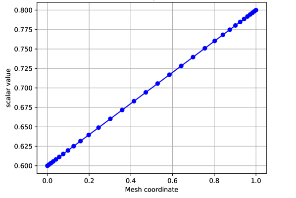
(a) Heat equation with $u(0)=0.6$ and $u(L)=0.8$.

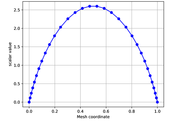
(b) Poiseuille flow with $k=1$.

Figure 1: Classical solutions for Heat equation and Poiseuille test cases with $n_{t}=32$, $n_{c}=12$ and $r=1.2$.

4.2 2D test cases

The 2D test conditions are chosen to exercise the range of boundary conditions.

4.2.1 Double repeating

Double repeating boundary conditions in the $x$ and $y$ directions are representative of modelling identical Taylor Green vortices [21] in an unbounded 2D domain. The actual modelling of the vortices requires the full Navier-Stokes equations. However, the Laplacian operator is indicative of the Poisson equation used to solve for the pressure in an incompressible CFD solver. In these cases the mesh is uniform as shown in Figure 2.

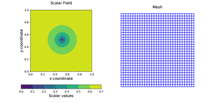
Figure 2: Solution and mesh for the solution of a 2D Laplacian with double repeating boundary conditions on 32x32 mesh.

Without any modification, the double repeating Laplacian is degenerate and cannot be solved classically. If the solution is part of a pressure correction solver, then it is only gradients of the solution that are important and the Laplacian can be modified at a single point (i.e. row) to have a Dircichlet condition that removes the degeneracy. The choice of point is an arbitrary user input via the setting of degfix on line 12 of LABEL:lst-input1. In Figure 2, the fixed point is set at the coordinates (16,16).

For quantum solvers, the normalisation of the state vector also removes the degeneracy and L-QLES has the option to generate Laplacians with and without the degeneracy. As shown in Appendix A, the degenerate Laplacian is the same when generated by Kronecker sums or direct discretisation. This is the only case for which this is true and provides a useful case for comparing with previous work.

4.2.2 Double Neumann

Double Neumann conditions provide a further sophistication of pressure correction type equations. Here, the Laplacian is generated on the same mesh as used for the momentum equations and, hence, is clustered next to boundary walls. This is shown in Figure 3 which is representative of a wall bounded cavity.

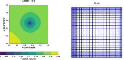
Figure 3: Solution and mesh for the solution of a 2D Laplacian with double Neumann boundary conditions on 32x32 mesh.

At a solid wall, the normal gradient of pressure is zero and the Neumann condition is used on all sides. As with the double repeating boundary conditions, this leads to a degenerate Laplacian and the same fix is used.

4.2.3 Double Dirichlet

Double Dirichlet conditions provide a more standard Laplacian test case with all the boundary values set to a constant. The same meshes as used as for the double Neumann case with clustering next to boundary walls. This is shown in Figure 4 which is representative of a wall bounded cavity.

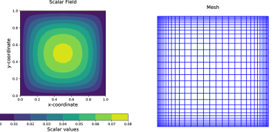
Figure 4: Solution and mesh for the solution of a 2D Laplacian with double Dirichlet boundary conditions on 32x32 mesh.

4.2.4 Wall bounded channel

A wall bounded flow with a Dirichelet inlet and a Neumann outlet is representative of Stokes flow in a channel. Stokes flow ia a very low speed flow where the copnvective terms in the Navier Stokes equation can be neglected. As before, this test case is only indicative of the Laplacian for the Navier Stokes stress tensor with constant viscosity. Since this is a channel flow the length and number of points in each direction are different as shown in Figure 5. Under the influence of a constant bulk force, the solution at the exit ($x=2$) approaches the fully developed Poiseuille flow profile.

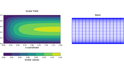
Figure 5: Solution and mesh for the solution of a 2D Laplacian for a wall bounded channel on a 16x32 mesh.

4.2.5 Test conditions

The mesh parameters for the double repeat, Neumann and Dirichlet test cases are shown in Table 3. For the repeat conditions, setting $r=1.0$ ensures there is no clustering.

Mesh	$n_{t}$	$n_{c}$	$r$ (Repeat)	$r$ (Neumann/Dirichlet)
4x4	4	2	1.0	1.4
8x8	8	3	1.0	1.3
16x16	16	6	1.0	1.3
32x32	32	12	1.0	1.2
64x64	64	22	1.0	1.2

Table 3: Suggested test conditions for 2D Repeat and Neumann Laplacians. Clustering parameters are the same in both $x$ and $y$ directions.

Table 4 gives suggested mesh parameters for the wall bounded flow Laplacians.

	$x$-direction			$y$-direction
Mesh	$n_{t}$	$n_{c}$	$r$	$n_{t}$	$n_{c}$	$r$
4x8	4	2	1.0	8	4	1.3
8x16	8	3	1.0	16	6	1.3
16x32	16	6	1.0	32	12	1.2
32x64	32	12	1.0	64	22	1.2

Table 4: Suggested test conditions for 2D wall bounded Laplacians.

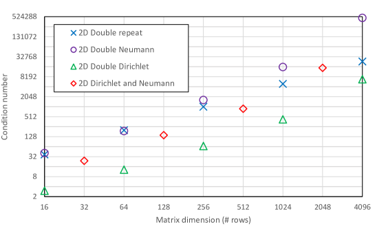
Figure 6: Condition numbers for the 2D Laplacians.

Figure 6 shows the condition numbers for all the 2D test cases. These range from $O(1)$ to $O(10^{5})$. For the smaller meshes, the double repeat and double Neumann cases have similar condition numbers as the clustering has only a small effect on the mesh. For the largest meshes the clustering has a larger effect on the condition numbers. Note that the condition numbers are only available for the non-degenerate Laplacians.

The condition numbers for the double Dirichlet cases are significantly lower than the other cases and provide the best option for initial evaluations.

4.3 3D test cases

Each of the 2D test cases can be easily extended into 3 dimensions. Here, two channel flow cases are considered with meshes of 4x8x8 and 8x16x16. The Laplacian condition numbers are 23 and 93 respectively.

Table 5 gives suggested mesh parameters for the wall bounded flow Laplacians.

	$x$-direction			$y$-direction			$z$-direction
Mesh	$n_{t}$	$n_{c}$	$r$	$n_{t}$	$n_{c}$	$r$	$n_{t}$	$n_{c}$	$r$
4x8x8	4	2	1.0	8	3	1.3	8	3	1.3
8x16x16	8	3	1.0	16	6	1.3	16	6	1.3

Table 5: Suggested test conditions for 3D wall bounded Laplacians.

5 Sample results

To illustrate the use of L-QLES, a brief study has been performed to analyse how different Laplacians affect the performance of two matrix encoding formulations.

The first is the Prepare-Select encoding [22, 23, 24, 25] where the Laplacian is expressed as a Linear Combination of Unitaries (LCU). Each unitary is typically a tensor product of 2x2 Pauli matrices, often referred to as a Pauli string. Each Pauli string is multiplied by a coefficient determined by the LCU decomposition. For real valued coefficients, the Laplacian, $L$ must be Hermitian. If it is not Hermitian, the LCU is applied to the bipartite matrix:

$$\begin{pmatrix}0&L\\ L^{*}&0\\ \end{pmatrix}$$ (10)

This requires an additional qubit in the select register.

The second encoding is the FABLE method [8]. FABLE is derived from the matrix encoding using a row-column oracle [26] which creates multiplexed rotations on an ancilla qubit for each entry in the matrix. FABLE uses Gray code ordering to convert the multiplexed rotations into an interleaving sequence of uncontrolled rotations and CNOT gates [27]. A linear system is solved to obtain the uncontrolled rotation angles from the original angles. Under certain circumstances a large number of these angles are zero, or close to zero, and the FABLE circuit is far shallower that the oracle based circuit. FABLE can encode non-Hermitian matrices.

In order to compare the performance of Pauli (Prep-Select) and FABLE a means of normalising their outputs is needed. For Prep-Select the number of non-zero entries in the Laplacian is used. For FABLE, the total number of entries in the matrix ($4^{n}$) is used as the row-column oracle creates a multiplexed rotation for every matrix position. In the following analysis, only the rotation gates in the FABLE encoding are used in the comparisons.

Note that all the FABLE calculations were run with a angle tolerance of $10^{-9}$. This is to eliminate rounding errors in the double precision Python matrix assembly calculations. Effectively the approximation part of the FABLE algorithm is not being used. Similarly, the LCU decomposition into Pauli strings can be subject to rounding error and strings with coefficients less than $10^{-9}$ are also ignored. Changing the tolerances will undoubtedly affect the results below but that is beyond the scope of this work which is to demonstrate the uses to which the testing framework can be put. The impact of changing the tolerance is not just the effect on circuit depth but the fidelity of the QLES solution.

5.1 1D Dirichlet and repeating

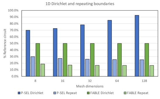
Figure 7: Normalised circuit counts for 1D Laplacian with Dirichlet and repeat cases.

Figure 7 compares the normalised Pauli and FABLE encoding for the 1d Laplacian with Dirichlet and repeating boundary conditions. The latter uses the degenerate version of the Laplacian. Both FABLE results (dark and light green) match those reported by [8].

5.2 2D Double repeating

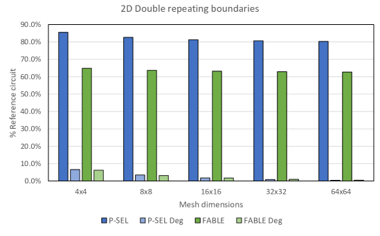
Figure 8: Normalised circuit counts for 2D double repeat case with and without degeneracy.

Figure 8 compares the normalised Pauli and FABLE encoding for the 2d double repeating case with degenerate and non-degenerate Laplacians. The degenerate FABLE results (light green) match those for the 4x4 and 8x8 Laplacians reported by [8], as expected since the Laplacians are identical. The Prep-Select encoding shows almost identical behaviour to FABLE for the degenerate Laplacian. For the 64x64 mesh, both encodings have a normalised count of 0.5%.

However, when the degeneracy is removed, the behaviour is quite different. Prep-Select encoding (dark blue) has a count of around 80% and FABLE has a count of around 60% for all meshes. It is striking that a modification to one row can cause such a significant change to both schemes.

	Prep-Select		FABLE
Mesh	non-deg	deg	non-deg	deg
4x4	12	8	9	9
8x8	16	11	13	13
16x16	20	14	17	17
32x32	24	17	21	21
64x64	28	20	25	25

Table 6: Total number of qubits used to encode for 2D double repeat Laplacians.

Table 6 shows the total number of qubits needed by each encoder. Since FABLE processes all the elements in the Laplacian, the number of qubits is independent of the gate count. In contrast, the Prep operator is a state loader for the LCU coefficients and the number of qubits needed depends on the number of coefficients to be loaded.

5.3 2D Double Neumann

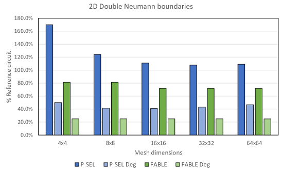
Figure 9: Normalised circuit counts for 2D double Neumann case with and without degeneracy.

Figure 9 compares the normalised Pauli and FABLE encoding for the 2d double Neumann case with degenerate and non-degenerate Laplacians. The behaviour is quite different to the double repeat case. Two changes have been made: the boundary condition and the clustering of the mesh. Testing the 16x16 mesh with a uniform mesh gave identical results for FABLE and for Prep-Select the count percentage reduced from 111% to 102%. The boundary condition is having the largest effect.

Taking the 4x4 mesh, the degenerate double repeat Laplacian, effectively, has 16 interior nodes, one of which is updated to remove the degeneracy. The double Neumann mesh has 4 interior nodes and 12 boundary nodes with one of the interior nodes being updated to remove the degeneracy. This gives a far more irregular sparsity pattern for the encoders to exploit. The different nature of the interior and boundary equations also means the degenerate Laplacians do not achieve the same reductions as the double repeat cases. It is surprising that the effect of the irregularity does not diminish.

	Prep-Select		FABLE
Mesh	non-deg	deg	non-deg	deg
4x4	12	10	9	9
8x8	16	14	13	13
16x16	20	18	17	17
32x32	24	22	21	21
64x64	28	27	25	25

Table 7: Total number of qubits used to encode for 2D double Neumann Laplacians.

Table 7 shows the total number of qubits needed by each encoder. Section 4.2.2 described this case as representative of a CFD pressure correction equation. In staggered-grid pressure correction formulations [28], the Neumann boundary condition becomes implicit and there are no boundary nodes in the Laplacian.

5.4 2D Double Dirichlet

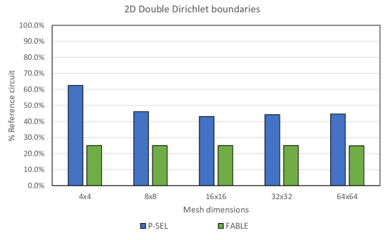
Figure 10: Normalised circuit counts for 2D double Dirichlet case.

Given the difference in behaviour between the double repeat and the double Neumann cases, the clustered Neumann meshes were also analysed using Dirichlet conditions on all boundaries. There is no degeneracy to be removed in this case. Figure 9 compares the normalised Pauli and FABLE encoding for the 2D double Dirichlet cases.

For Prep-Select, the number of Pauli strings in the LCU was identical to those in Figure 9. The FABLE counts were almost identical, with differences of less than 0.1%.

5.5 2D Wall bounded channel

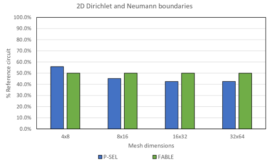
Figure 11: Normalised circuit counts for 2D wall bounded channel.

Figure 11 compares the normalised Pauli and FABLE encoding for the wall bounded channel. The FABLE results consistently have a 50% count for all the cases. There is some variation in the Prep-Select counts which settles to around 40% for the higher meshes.

Mesh	Prep-Select	FABLE
4x8	12	11
8x16	16	15
16x32	20	19
32x64	24	23

Table 8: Total number of qubits used to encode for 2D wall bounded Laplacians.

Table 8 shows the total number of qubits needed by each encoder. The difference between Prep-Select and FABLE is only 1 qubit, which is lower than previous cases where the non-degenerate cases differed by 3 qubits.

5.6 3D Wall bounded channel

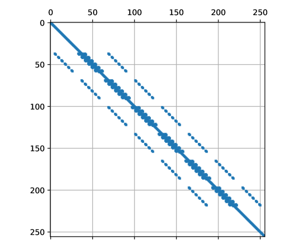
(a) Coordinate based ordering.

(b) Shell based ordering.

Figure 12: Sparsity patterns for 4x8x8 3D Laplacian.

The 3D test case is used to demonstrate the effect of reordering on each encoder. Figure 12 shows the sparsity patterns of the original and reordered Laplacians.

			Original			Reordered
Mesh	$\kappa$	non-zeros	Pauli strings	count	qubits	Pauli strings	count	qubits
4x8x8	22.8	724	272	37.6%	18	8384	1158%	23
8x16x16	93.1	9300	2496	26.8%	24	-	-	-

Table 9: LCU and qubit counts for Prep-Select encoding for 3D wall bunded flows.

Table 9 shows the number of Pauli strings and qubits for the original and reordered Laplacians. Firstly, the Pauli string counts are lower than for the 2D cases. However, the reordering has a huge effect, increasing the number of Pauli strings by over a factor of over 30 for the 4x8x8 mesh. Processing of the 8x16x16 mesh was not attempted.

In contrast the FABLE counts for the original and reordered Laplacians were 25% and 100% for both cases. Whilst the row-column oracle produces the same set of rotation angles, they are in a different order. This in turn changes the derived angles and/or their Gray code order.

6 Closing remarks

A test case framework, L-QLES, has been presented which contains important features of industrial applications of sparse matrix algebra. Sample test cases have demonstrated the flexibility to investigate features of quantum algorithms, in this case matrix encoding. With some differences in degree, all the 2D cases show asymptotic behaviour as the mesh dimensions increase. This suggests progress on encoding schemes can be made on smaller meshes. Other aspects of QLES have not been investigated but the rate of increase of condition number with mesh size demonstrates the need to consider industrially representative cases.

An important part of any application of QLES is the classical preprocessing needed to prepare the quantum circuit. L-QLES also allows aspects such as matrix encoding to be evaluated. For example, the FABLE encoding of the 64x64 mesh took 20s, whereas the Prep-Select encoding took 6,639 seconds (1:50:33). Both were run on an Intel^® Core^© i9 12900K 3.2GHz Alder Lake 16 core processor with 64GB of 3,200MHz DDR4 RAM.

7 Data availability

The L-QLES scripts and sample input files are available from https://github.com/rolls-royce/qc-cfd/tree/main/L-QLES.

8 Acknowledgements

The idea for this test case framework arose in discussions with Christoph Sünderhauf and Joan Camps at their Riverlane offices and I am very grateful to them for their inspiration. I hope L-QLES meets our goal of allowing quantum algorithm developers to stress test their algorithms without the need for esoteric domain knowledge or reliance on matrices supplied by industry. I would also like to thank Jarrett Smalley and Tony Phipps of Rolls-Royce and Philippa Rubin of the STFC Hartree Centre for their helpful comments on this work.

The permission of Rolls-Royce to publish this work is gratefully acknowledged. This work was completed under funding received under the UK’s Commercialising Quantum Technologies Programme (Grant reference 10004857).

Appendix A Kronecker sums vs direct discretisation

For Cartesian lattice based meshes, a convenient way to create a 2D Laplacian operator, $L$ from separate 1D operators, $L_{xx}$ and $L_{yy}$ is using the Kronecker sum:

$$L=L_{yy}\oplus L_{xx}=I\otimes L_{xx}+L_{yy}\otimes I$$ (11)

The ordering of the sum depends on the indexing of the nodes in the resulting 2D lattice mesh. Figure 13 shows a 4x4 lattice. In the formulation of Equation 11, the $L_{xx}$ operator acts in the horizontal direction and $L_{yy}$ in the vertical direction.

Figure 13: Indexing of nodes on a 4x4 Cartesian lattice mesh.

The following subsections analyse how well the construction in Equation 11 preserves the relevant boundary conditions.

A.1 Repeat-Repeat boundary conditions

For a uniform mesh, the 1D Laplacian operator with repeating boundary conditions is:

$$L_{xx}=L_{yy}=\begin{pmatrix}[r]a&-b&.&-b\\ -b&a&-b&.\\ .&-b&a&-b\\ -b&.&-b&a\\ \end{pmatrix}$$ (12)

Many analyses use $a=1$ and $b=0.5$, but this does not have to be the case. Note that this is not the usual CFD formulation where the values on opposite sides of the repeating boundary are equal. This formulation can be envisaged by taking the bottom line of the lattice in Figure 13 and placing a nodes at positions (-1, 0) and (4,0) with the same uniform spacing as the rest of the lattice. Here, the indices refer to (x,y) coordinate positions. The repeating boundary condition sets, $\phi_{3,0}=\phi_{-1,0}$ and $\phi_{0,0}=\phi_{4,0}$. This is an important distinction as the two formulations have different periods.

If repeating conditions are applied in both the $x$ and $y$ directions, the 2D Laplacian constructed by using Equation 11 is:

$$L\ket{\phi}=\\ \setcounter{MaxMatrixCols}{16}\begin{pmatrix}2a&-b&.&-b&-b&.&.&.&.&.&.&.&-b&.&.&.\\ -b&2a&-b&.&.&-b&.&.&.&.&.&.&.&-b&.&.\\ .&-b&2a&-b&.&.&-b&.&.&.&.&.&.&.&-b&.\\ -b&.&-b&2a&.&.&.&-b&.&.&.&.&.&.&.&-b\\ -b&.&.&.&2a&-b&.&-b&-b&.&.&.&.&.&.&.\\ .&-b&.&.&-b&2a&-b&.&.&-b&.&.&.&.&.&.\\ .&.&-b&.&.&-b&2a&-b&.&.&-b&.&.&.&.&.\\ .&.&.&-b&-b&.&-b&2a&.&.&.&-b&.&.&.&.\\ .&.&.&.&-b&.&.&.&2a&-b&.&-b&-b&.&.&.\\ .&.&.&.&.&-b&.&.&-b&2a&-b&.&.&-b&.&.\\ .&.&.&.&.&.&-b&.&.&-b&2a&-b&.&.&-b&.\\ .&.&.&.&.&.&.&-b&-b&.&-b&2a&.&.&.&-b\\ -b&.&.&.&.&.&.&.&-b&.&.&.&2a&-b&.&-b\\ .&-b&.&.&.&.&.&.&.&-b&.&.&-b&2a&-b&.\\ .&.&-b&.&.&.&.&.&.&.&-b&.&.&-b&2a&-b\\ .&.&.&-b&.&.&.&.&.&.&.&-b&-b&.&-b&2a\\ \end{pmatrix}\begin{pmatrix}\phi_{0}\\ \phi_{1}\\ \phi_{2}\\ \phi_{3}\\ \phi_{4}\\ \phi_{5}\\ \phi_{6}\\ \phi_{7}\\ \phi_{8}\\ \phi_{9}\\ \phi_{10}\\ \phi_{11}\\ \phi_{12}\\ \phi_{13}\\ \phi_{14}\\ \phi_{15}\\ \end{pmatrix}$$ (13)

The matrix is shown acting on a vector to aid visual inspection that the correct 2D Laplacian has been constructed. Doubly repeating boundary conditions such as this are relevant to CFD for test cases such as the Taylor-Green Vortex [29] and the decay of isotropic turbulence [30].

A.2 Dirichlet-Dirichlet boundary conditions

For a uniform mesh, the 1D Laplacian operator with Dirichlet boundary conditions at each end is:

$$L_{xx}=L_{yy}=\begin{pmatrix}[r]a&.&.&.\\ -b&a&-b&.\\ .&-b&a&-b\\ .&.&.&a\\ \end{pmatrix}$$ (14)

If Dirichlet boundary conditions are applied in both the $x$ and $y$ directions, the 2D Laplacian constructed by using Equation 11 is:

$$L\ket{\phi}=\\ \setcounter{MaxMatrixCols}{16}\begin{pmatrix}2a&.&.&.&.&.&.&.&.&.&.&.&.&.&.&.\\ -b&2a&-b&.&.&.&.&.&.&.&.&.&.&.&.&.\\ .&-b&2a&-b&.&.&.&.&.&.&.&.&.&.&.&.\\ .&.&.&2a&.&.&.&.&.&.&.&.&.&.&.&.\\ -b&.&.&.&2a&.&.&.&-b&.&.&.&.&.&.&.\\ .&-b&.&.&-b&2a&-b&.&.&-b&.&.&.&.&.&.\\ .&.&-b&.&.&-b&2a&-b&.&.&-b&.&.&.&.&.\\ .&.&.&-b&.&.&.&2a&.&.&.&-b&.&.&.&.\\ .&.&.&.&-b&.&.&.&2a&.&.&.&-b&.&.&.\\ .&.&.&.&.&-b&.&.&-b&2a&-b&.&.&-b&.&.\\ .&.&.&.&.&.&-b&.&.&-b&2a&-b&.&.&-b&.\\ .&.&.&.&.&.&.&-b&.&.&.&2a&.&.&.&-b\\ .&.&.&.&.&.&.&.&.&.&.&.&2a&.&.&.\\ .&.&.&.&.&.&.&.&.&.&.&.&-b&2a&-b&.\\ .&.&.&.&.&.&.&.&.&.&.&.&.&-b&2a&-b\\ .&.&.&.&.&.&.&.&.&.&.&.&.&.&.&2a\\ \end{pmatrix}\begin{pmatrix}\phi_{0}\\ \phi_{1}\\ \phi_{2}\\ \phi_{3}\\ \phi_{4}\\ \phi_{5}\\ \phi_{6}\\ \phi_{7}\\ \phi_{8}\\ \phi_{9}\\ \phi_{10}\\ \phi_{11}\\ \phi_{12}\\ \phi_{13}\\ \phi_{14}\\ \phi_{15}\\ \end{pmatrix}$$ (15)

From inspection of Equation 15, we can see that the corner nodes 0, 3, 12 and 15 have the correct boundary condition; and, the interior nodes 5, 6, 9 and 10 have the correct Laplacian operator. The remaining boundary nodes 1, 2, 4, 7, 8, 11, 13 and 14 do not have the Dirichlet boundary condition correctly applied. Each of these rows in the matrix should have a single entry $2a$ on the diagonal, as shown in Equation 16. This matrix has few off diagonal entries due to the small ratio of internal nodes to boundary nodes. For larger meshes, the number of internal nodes is dominant.

$$L\ket{\phi}=\\ \setcounter{MaxMatrixCols}{16}\begin{pmatrix}2a&.&.&.&.&.&.&.&.&.&.&.&.&.&.&.\\ .&2a&.&.&.&.&.&.&.&.&.&.&.&.&.&.\\ .&.&2a&.&.&.&.&.&.&.&.&.&.&.&.&.\\ .&.&.&2a&.&.&.&.&.&.&.&.&.&.&.&.\\ .&.&.&.&2a&.&.&.&.&.&.&.&.&.&.&.\\ .&-b&.&.&-b&2a&-b&.&.&-b&.&.&.&.&.&.\\ .&.&-b&.&.&-b&2a&-b&.&.&-b&.&.&.&.&.\\ .&.&.&.&.&.&.&2a&.&.&.&.&.&.&.&.\\ .&.&.&.&.&.&.&.&2a&.&.&.&.&.&.&.\\ .&.&.&.&.&-b&.&.&-b&2a&-b&.&.&-b&.&.\\ .&.&.&.&.&.&-b&.&.&-b&2a&-b&.&.&-b&.\\ .&.&.&.&.&.&.&.&.&.&.&2a&.&.&.&.\\ .&.&.&.&.&.&.&.&.&.&.&.&2a&.&.&.\\ .&.&.&.&.&.&.&.&.&.&.&.&.&2a&.&.\\ .&.&.&.&.&.&.&.&.&.&.&.&.&.&2a&.\\ .&.&.&.&.&.&.&.&.&.&.&.&.&.&.&2a\\ \end{pmatrix}\begin{pmatrix}\phi_{0}\\ \phi_{1}\\ \phi_{2}\\ \phi_{3}\\ \phi_{4}\\ \phi_{5}\\ \phi_{6}\\ \phi_{7}\\ \phi_{8}\\ \phi_{9}\\ \phi_{10}\\ \phi_{11}\\ \phi_{12}\\ \phi_{13}\\ \phi_{14}\\ \phi_{15}\\ \end{pmatrix}$$ (16)

Dirichet boundary conditions of this type are relevant to fully wall bounded flows such as lid driven cavities [31]. However, the construction if Equation 11 clearly produces the wrong 2-dimensional operator.

A.3 Dirichlet-Neumann boundary conditions

A more typical CFD test case is the flow between two parallel plates with a Dirichlet inflow and a Neumann outflow condition. If in Figure 13, the flow is from left to right, then $L_{yy}$ is as in Equation 14 and

$$L_{xx}=\begin{pmatrix}[r]a&.&.&.\\ -b&a&-b&.\\ .&-b&a&-b\\ .&.&-a&a\\ \end{pmatrix}$$ (17)

The corresponding 2D Laplace operator is:

$$L\ket{\phi}=\\ \setcounter{MaxMatrixCols}{16}\begin{pmatrix}2a&.&.&.&.&.&.&.&.&.&.&.&.&.&.&.\\ -b&2a&-b&.&.&.&.&.&.&.&.&.&.&.&.&.\\ .&-b&2a&-b&.&.&.&.&.&.&.&.&.&.&.&.\\ .&.&-a&2a&.&.&.&.&.&.&.&.&.&.&.&.\\ -b&.&.&.&2a&.&.&.&-b&.&.&.&.&.&.&.\\ .&-b&.&.&-b&2a&-b&.&.&-b&.&.&.&.&.&.\\ .&.&-b&.&.&-b&2a&-b&.&.&-b&.&.&.&.&.\\ .&.&.&-b&.&.&-a&2a&.&.&.&-b&.&.&.&.\\ .&.&.&.&-b&.&.&.&2a&.&.&.&-b&.&.&.\\ .&.&.&.&.&-b&.&.&-b&2a&-b&.&.&-b&.&.\\ .&.&.&.&.&.&-b&.&.&-b&2a&-b&.&.&-b&.\\ .&.&.&.&.&.&.&-b&.&.&-a&2a&.&.&.&-b\\ .&.&.&.&.&.&.&.&.&.&.&.&2a&.&.&.\\ .&.&.&.&.&.&.&.&.&.&.&.&-b&2a&-b&.\\ .&.&.&.&.&.&.&.&.&.&.&.&.&-b&2a&-b\\ .&.&.&.&.&.&.&.&.&.&.&.&.&.&-a&2a\\ \end{pmatrix}\begin{pmatrix}\phi_{0}\\ \phi_{1}\\ \phi_{2}\\ \phi_{3}\\ \phi_{4}\\ \phi_{5}\\ \phi_{6}\\ \phi_{7}\\ \phi_{8}\\ \phi_{9}\\ \phi_{10}\\ \phi_{11}\\ \phi_{12}\\ \phi_{13}\\ \phi_{14}\\ \phi_{15}\\ \end{pmatrix}$$ (18)

Now, only the corner nodes 0 and 12 on the inflow boundary are correct. The interior nodes 5, 6, 9 and 10 are also still correct. Nodes 1, 2 and 3 on the lower wall and 12, 14 and 15 on the upper wall can be corrected as before. At the inflow nodes 4 and 8 and the outflow nodes 7 and 11, there is a question of whether to include the shear terms, i.e. the gradients in the y-direction. It is usual to ignore these at the inlet where it is desirable to ensure that the specified boundary values are achieved. For wall-bounded flows, the shear terms are usually retained at the outlet to ensure boundary layers on the walls do not see a discontinuity in the forces acting on the flow. At junctions of Dirichlet and Neumann boundary conditions, it is usual for the Dirchlet condition to take precedence. With these considerations the correct Laplacian is:

$$L\ket{\phi}=\\ \setcounter{MaxMatrixCols}{16}\begin{pmatrix}2a&.&.&.&.&.&.&.&.&.&.&.&.&.&.&.\\ .&2a&.&.&.&.&.&.&.&.&.&.&.&.&.&.\\ .&.&2a&.&.&.&.&.&.&.&.&.&.&.&.&.\\ .&.&.&2a&.&.&.&.&.&.&.&.&.&.&.&.\\ .&.&.&.&2a&.&.&.&.&.&.&.&.&.&.&.\\ .&-b&.&.&-b&2a&-b&.&.&-b&.&.&.&.&.&.\\ .&.&-b&.&.&-b&2a&-b&.&.&-b&.&.&.&.&.\\ .&.&.&-b&.&.&-a&2a&.&.&.&-b&.&.&.&.\\ .&.&.&.&.&.&.&.&2a&.&.&.&.&.&.&.\\ .&.&.&.&.&-b&.&.&-b&2a&-b&.&.&-b&.&.\\ .&.&.&.&.&.&-b&.&.&-b&2a&-b&.&.&-b&.\\ .&.&.&.&.&.&.&-b&.&.&-a&2a&.&.&.&-b\\ .&.&.&.&.&.&.&.&.&.&.&.&2a&.&.&.\\ .&.&.&.&.&.&.&.&.&.&.&.&.&2a&.&.\\ .&.&.&.&.&.&.&.&.&.&.&.&.&.&2a&.\\ .&.&.&.&.&.&.&.&.&.&.&.&.&.&.&2a\\ \end{pmatrix}\begin{pmatrix}\phi_{0}\\ \phi_{1}\\ \phi_{2}\\ \phi_{3}\\ \phi_{4}\\ \phi_{5}\\ \phi_{6}\\ \phi_{7}\\ \phi_{8}\\ \phi_{9}\\ \phi_{10}\\ \phi_{11}\\ \phi_{12}\\ \phi_{13}\\ \phi_{14}\\ \phi_{15}\\ \end{pmatrix}$$ (19)

A.4 Toplitz boundary conditions

The Toeplitz style of Laplace operator, Equation 20, does not correspond to a commonly used CFD boundary condition and is not analysed further.

$$L_{xx}=\begin{pmatrix}[r]a&-b&.&.\\ -b&a&-b&.\\ .&-b&a&-b\\ .&.&-b&a\\ \end{pmatrix}$$ (20)

A.5 Summary

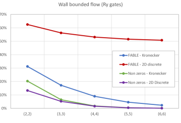
Figure 14: Percentage of rotation gates in a FABLE circuit for Dirichlet-Neumann boundary conditions using Kronecker sum and direct discretisation. (nx, ny) the are number of qubits in x and y directions. Also shown is percentage of non-zeros in each matrix formulation.

Figure 14 shows the impact of the matrix formulation on the number or rotation gates in a FABLE circuit. The notation follows [8] where the abscissa is labelled (nx, ny) and nx and ny are the number of qubits in x and y directions. E.g., (6,6) corresponds to a 64x64 mesh and, hence, a 4,096x4,096 sparse matrix. The percentages are relative the to full circuit encoding of all the entries in the matrix, i.e. 16,777,216 rotation gates for the (6,6) case. Figure 14 also shows the percentage of non-zero entries in the matrix. The effect of the different boundary treatments is visible in the (2,2) case as the number of boundary nodes is larger than the number of interior nodes. Otherwise the percentages are dominated by the number of interiors nodes.

Appendix B Clustering the mesh points

Mesh clustering is generally applied normal to a wall and can, therefore, be considered as a 1-dimensional operation. Users generally wish to control the near wall spacing, the rate of expansion away from the wall and the spacing in freestream region where the mesh is uniform. Additionally, the transition between the clustered and freestream regions should be smooth. Depending on how the latter is defined can result in a over-prescribed set of equations. L-QLES enforces smoothness at the expense of setting the near-wall spacing. This simplifies the solution of the clustering equations which is preferred for the QLES experiments for which the code is intended.

The input parameters required for the mesh clustering are:

• $L$, the total extent of the mesh,

• $n_{t}$, the total number of mesh points,

• $n_{c}$, the number of points in each clustered region,

• $r$, the expansion ratio in the cluster region,

• $C_{type}$, flag for 1 or 2 sided clustering.

For 2-sided clustering, the number of points in the uniform freestream region, $n_{u}$ is:

$$n_{u}=n_{t}-2n_{c}+2$$ (21)

The $+2$ on the right side arise because the transition nodes between the clustered and uniform regions are counted twice when solving for the mesh distribution.

Defining $D$ as the freestream spacing, $C$ as the width of each clustered region and $d$ as the near wall spacing gives:

$$\sum_{i=0}^{n_{c}-2}r^{i}d=\frac{r^{n_{c}-1}-1}{r-1}d=C$$ (22)

$$L=(n_{u}-1)D+2C$$ (23)

$$r^{n_{c}-1}d=D$$ (24)

Where Equation 24 is the requirement that the transition from the clustered region to the uniform region is smooth. Solving the above equations results in the mesh distribution:

$$x=\begin{pmatrix}0\\ d\\ d+rd\\ \vdots\\ C\\ C+D\\ \vdots\\ C+(n_{u}-1)D\\ \vdots\\ L-rd\\ L-d\\ L\end{pmatrix}$$ (25)

For 1-sided clustering, $n_{u}=n_{t}-n_{c}+1$ and $L=(n_{u}-1)D+C$. Figure 15 shows a sample 2-sided mesh distribution and spacing.

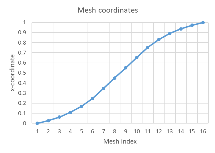
(a) Mesh coordinates.

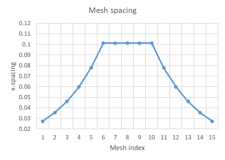
(b) Mesh spacing.

Figure 15: Mesh coordinates and spacing for $n_{t}=16$, $n_{c}=6$, $r=1.3$ and $L=1.0$.

Appendix C Running L-QLES

The options for running L-QLES can be obtained by using the -h option on the command line to give:

l-qles.py -i <input file> {-c <x,y,z>} {-d} {-e} {-h} {-j} {-m} {-r} {-s}

     -i {name of input file}
     -c {x,y,z} cut slice of 3D solution to be plotted, default = x
     -d allow degnerate matrices, default = False
     -e calculate eigenvalues and condition number, default = False
     -h help menu
     -j split plots into separate windows for saving, default is single window
     -m plot matrix, default = False
     -r reorder matrix and RHS to use shell ordering of mesh, default = False
     -s plot solutons and mesh, default = False

The structure of the input XML file is described in Section 3. The sample data files in the GitHub repository have additional comments to aid understanding.

C.1 Command line options

The default for all options is off unless otherwise stated.

-i

Followed by the name of the XML input file. There is no default.

-c

Followed by x, y or z. For 3D cases this indicates which cutting plane is used to show the solution if the option -s is turned on. The cutting plane is position at the mid-point of the domain and default is an x plane.

-d

As discussed in Section 4.2.1, Laplacians that consist entirely of repeating and/or Neumann boundaries are degenerate. The default is to remove the degeneracy by applying a Dirichlet condition at a single point in the mesh determined by the input variable degfix. Since other authors have used the degenerate form, this option does not apply the degeneracy fix so that like with like comparisons can be made. Note that L-QLES cannot solve a degenerate Poisson equation and no solution file is stored in these cases. Other files have _d appended to their case name.

-e

Calculate the eigenvalues and condition number of the Laplacian. This scales with $O(N^{3})$ where $N$ is the dimension of the matrix and so can only be used with small matrices. As Table 1 shows, L-QLES allows a wide range of condition numbers to be produced using small meshes.

-h

Display help menu.

-j

The default for the -m and -s plotting options is to create figures with 2 plots per pane. This option plots each figure separately which may be useful when preparing reports.

-m

Plot the matrix values and sparsity pattern using the Matplotlib [32] imshow and spy options.

-r

Applies the shell reordering described in Section 3.3. If this option is on, all files have _r appended to their case name. If the dengeneracy and reordering options are both on, then _d_r is appended to the case name.

-s

Plot the mesh and contours of the solution variable.

C.2 Output files

Note the Laplacian, $L$, is normalised to have $||L||_{max}=1$ with the same scale factor applied to the RHS state to ensure that the solution state corresponds to the original problem. This does not mean that the RHS state is normalised.

L-QLES outputs 2 types of files: Python and C/C++ compatible binary files:

Laplacian

This is stored using the compressed sparse row format. The name of the Python file is casename_mat.npz and the C/C++ binary file is casename_mat.bin.

RHS vector

The right-hand side vector contains the boundary values and the bulk inhomogeneous force term. The name of the Python file is casename_rhs.npy and the C/C++ binary file is casename_rhs.bin.

Solution vector

If the Laplacian is not degenerate, the solution vector is output. The name of the Python file is casename_sol.npy and the C/C++ binary file is casename_sol.bin.

Reordering matrix

If the reordering option has been used then the column-wise permutation matrix ($Q$ in Equation 4) is written to the files casename_ord.npz and casename_ord.bin. As described in Section 3.3, this matrix is needed to recover the solution to the original Laplacian from the solution to the reordered one.

If the-r and/or -d options have been used, the case name is amended as described above.

References

- [1] T. Hoefler, T. Häner, and M. Troyer, “Disentangling hype from practicality: on realistically achieving quantum advantage,” Communications of the ACM, vol. 66, no. 5, pp. 82–87, 2023.
- [2] J. D. Denton, “Lessons from rotor 37,” Journal of Thermal Science, vol. 6, pp. 1–13, 1997.
- [3] L. Reid and R. D. Moore, “Design and overall performance of four highly loaded, high speed inlet stages for an advanced high-pressure-ratio core compressor,” Tech. Rep. NASA-TP-1337, NASA, 1978.
- [4] D. Levy, R. Wahls, T. Zickuhr, J. Vassberg, S. Agrawal, S. Pirzadeh, and M. Hemsch, “Summary of data from the first aiaa cfd drag prediction workshop,” in 40th AIAA Aerospace Sciences Meeting & Exhibit, p. 841, 2002.
- [5] E. N. Tinoco, O. P. Brodersen, S. Keye, K. R. Laflin, E. Feltrop, J. C. Vassberg, M. Mani, B. Rider, R. A. Wahls, J. H. Morrison, et al., “Summary data from the sixth aiaa cfd drag prediction workshop: Crm cases,” Journal of Aircraft, vol. 55, no. 4, pp. 1352–1379, 2018.
- [6] L. Lapworth, “A hybrid quantum-classical cfd methodology with benchmark hhl solutions,” arXiv preprint arXiv:2206.00419, 2022.
- [7] A. M. Childs, R. Kothari, and R. D. Somma, “Quantum algorithm for systems of linear equations with exponentially improved dependence on precision,” SIAM Journal on Computing, vol. 46, no. 6, pp. 1920–1950, 2017.
- [8] D. Camps and R. Van Beeumen, “Fable: Fast approximate quantum circuits for block-encodings,” in 2022 IEEE International Conference on Quantum Computing and Engineering (QCE), pp. 104–113, IEEE, 2022.
- [9] H.-L. Liu, Y.-S. Wu, L.-C. Wan, S.-J. Pan, S.-J. Qin, F. Gao, and Q.-Y. Wen, “Variational quantum algorithm for the poisson equation,” Physical Review A, vol. 104, no. 2, p. 022418, 2021.
- [10] Y. Sato, R. Kondo, S. Koide, H. Takamatsu, and N. Imoto, “Variational quantum algorithm based on the minimum potential energy for solving the poisson equation,” Physical Review A, vol. 104, no. 5, p. 052409, 2021.
- [11] M. Ali and M. Kabel, “Performance study of variational quantum algorithms for solving the poisson equation on a quantum computer,” Physical Review Applied, vol. 20, no. 1, p. 014054, 2023.
- [12] B. Daribayev, A. Mukhanbet, and T. Imankulov, “Implementation of the hhl algorithm for solving the poisson equation on quantum simulators,” Applied Sciences, vol. 13, no. 20, p. 11491, 2023.
- [13] C. Sünderhauf, E. Campbell, and J. Camps, “Block-encoding structured matrices for data input in quantum computing,” Quantum, vol. 8, p. 1226, 2024.
- [14] L. Lapworth, “Implicit hybrid quantum-classical cfd calculations using the hhl algorithm,” arXiv preprint arXiv:2209.07964, 2022.
- [15] A. W. Harrow, A. Hassidim, and S. Lloyd, “Quantum algorithm for linear systems of equations,” Physical review letters, vol. 103, no. 15, p. 150502, 2009.
- [16] A. Gilyén, Y. Su, G. H. Low, and N. Wiebe, “Quantum singular value transformation and beyond: exponential improvements for quantum matrix arithmetics,” arXiv preprint arXiv:1806.01838, 2018.
- [17] Y. Dong, X. Meng, K. B. Whaley, and L. Lin, “Efficient phase-factor evaluation in quantum signal processing,” Physical Review A, vol. 103, no. 4, p. 042419, 2021.
- [18] M. Darwish and F. Moukalled, The finite volume method in computational fluid dynamics: an advanced introduction with OpenFOAM® and Matlab®. Springer, 2016.
- [19] E. Cuthill and J. McKee, “Reducing the bandwidth of sparse symmetric matrices,” in Proceedings of the 1969 24th national conference, pp. 157–172, 1969.
- [20] M. Aftosmis, M. Berger, and S. Murman, “Applications of space-filling-curves to cartesian methods for cfd,” in 42nd AIAA Aerospace Sciences Meeting and Exhibit, p. 1232, 2004.
- [21] G. I. Taylor and A. E. Green, “Mechanism of the production of small eddies from large ones,” Proceedings of the Royal Society of London. Series A-Mathematical and Physical Sciences, vol. 158, no. 895, pp. 499–521, 1937.
- [22] A. M. Childs and N. Wiebe, “Hamiltonian simulation using linear combinations of unitary operations,” arXiv preprint arXiv:1202.5822, 2012.
- [23] R. Babbush, C. Gidney, D. W. Berry, N. Wiebe, J. McClean, A. Paler, A. Fowler, and H. Neven, “Encoding electronic spectra in quantum circuits with linear t complexity,” Physical Review X, vol. 8, no. 4, p. 041015, 2018.
- [24] D. W. Berry, A. M. Childs, R. Cleve, R. Kothari, and R. D. Somma, “Simulating hamiltonian dynamics with a truncated taylor series,” Physical review letters, vol. 114, no. 9, p. 090502, 2015.
- [25] D. W. Berry, M. Kieferová, A. Scherer, Y. R. Sanders, G. H. Low, N. Wiebe, C. Gidney, and R. Babbush, “Improved techniques for preparing eigenstates of fermionic hamiltonians,” npj Quantum Information, vol. 4, no. 1, pp. 1–7, 2018.
- [26] L. Lin, “Lecture notes on quantum algorithms for scientific computation,” arXiv preprint arXiv:2201.08309, 2022.
- [27] M. Mottonen, J. J. Vartiainen, V. Bergholm, and M. M. Salomaa, “Transformation of quantum states using uniformly controlled rotations,” arXiv preprint quant-ph/0407010, 2004.
- [28] H. K. Versteeg and W. Malalasekera, An introduction to computational fluid dynamics: the finite volume method. Pearson education, 2007.
- [29] S. A. Orszag, “Numerical simulation of the taylor-green vortex,” in Computing Methods in Applied Sciences and Engineering Part 2: International Symposium, Versailles, December 17–21, 1973, pp. 50–64, Springer, 1974.
- [30] G. Comte-Bellot and S. Corrsin, “Simple eulerian time correlation of full-and narrow-band velocity signals in grid-generated,‘isotropic’turbulence,” Journal of fluid mechanics, vol. 48, no. 2, pp. 273–337, 1971.
- [31] R. E. Smith Jr and A. Kidd, “Comparative study of two numerical techniques for the solution of viscous flow in a driven cavity,” NASA Special Publication, vol. 378, p. 61, 1975.
- [32] J. D. Hunter, “Matplotlib: A 2d graphics environment,” Computing in science & engineering, vol. 9, no. 03, pp. 90–95, 2007.