bears Make Neuro-Symbolic Models
Aware of their Reasoning Shortcuts

Abstract

Neuro-Symbolic (NeSy) predictors that conform to symbolic knowledge – encoding, e.g., safety constraints – can be affected by Reasoning Shortcuts (RSs): They learn concepts consistent with the symbolic knowledge by exploiting unintended semantics. RSs compromise reliability and generalization and, as we show in this paper, they are linked to NeSy models being overconfident about the predicted concepts. Unfortunately, the only trustworthy mitigation strategy requires collecting costly dense supervision over the concepts. Rather than attempting to avoid RSs altogether, we propose to ensure NeSy models are aware of the semantic ambiguity of the concepts they learn, thus enabling their users to identify and distrust low-quality concepts. Starting from three simple desiderata, we derive bears (BE Aware of Reasoning Shortcuts), an ensembling technique that calibrates the model’s concept-level confidence without compromising prediction accuracy, thus encouraging NeSy architectures to be uncertain about concepts affected by RSs. We show empirically that bears improves RS-awareness of several state-of-the-art NeSy models, and also facilitates acquiring informative dense annotations for mitigation purposes.

Keywords Neuro-Symbolic AI  $\cdot$ Uncertainty  $\cdot$ Reasoning Shortcuts  $\cdot$ Calibration  $\cdot$ Probabilistic Reasoning  $\cdot$ Concept-Based Models

1 Introduction

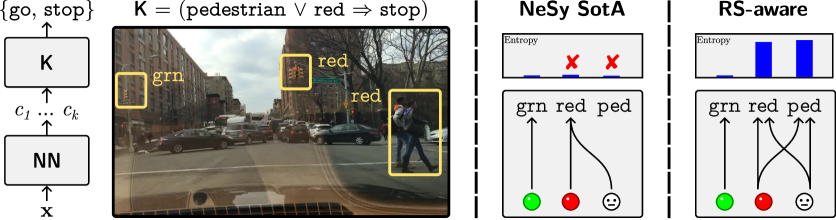
Figure 1:

bears lessens overconfidence due to reasoning shortcuts. Left: In the BDD-OIA

autonomous driving task (Xu et al., 2020; Sawada and Nakamura, 2022), NeSy predictors can attain high accuracy and comply with the knowledge even when confusing the concepts of pedestrian (${\tt ped}$) and red light (${\tt red}$) (Marconato et al., 2023a). Middle: State-of-the-art NeSy architectures predict concepts affected by RSs with high confidence, making it impossible to discriminate between reliable and unreliable concept predictions. Right: bears encourages them to allocate probability to conflicting concept maps, substantially lessening overconfidence.

Research in Neuro-Symbolic (NeSy) AI (Garcez et al., 2019; De Raedt et al., 2021; Garcez et al., 2022) has recently yielded a wealth of architectures capable of integrating low-level perception and symbolic reasoning. Crucially, these architectures encourage (Xu et al., 2018) or guarantee (Manhaeve et al., 2018; Giunchiglia and Lukasiewicz, 2020; Ahmed et al., 2022a; Hoernle et al., 2022) that their predictions conform to given prior knowledge encoding, e.g., structural or safety constraints, thus offering improved reliability compared to neural baselines (Di Liello et al., 2020; Hoernle et al., 2022; Giunchiglia and Lukasiewicz, 2020).

It was recently shown that, however, NeSy architectures can achieve high prediction accuracy by learning concepts – aka neural predicates (Manhaeve et al., 2018) – with unintended semantics (Marconato et al., 2023a; Li et al., 2023). E.g., consider an autonomous driving task like BDD-OIA (Xu et al., 2020) in which a model has to predict safe actions based on the contents of a dashcam image, under the constraint that whenever it detects pedestrians or red lights the vehicle must stop. Then, the model can achieve perfect accuracy and comply with the constraint even when confusing pedestrians for red lights, precisely because both entail the correct (stop) action (Marconato et al., 2023a). See Fig. 1 for an illustration.

These so-called reasoning shortcuts (RSs) occur because the prior knowledge and data may be insufficient to pin-down the intended semantics of all concepts, and cannot be avoided by maximizing prediction accuracy alone. They compromise in-distribution (Wang et al., 2023) and out-of-distribution generalization (Marconato et al., 2023a; Li et al., 2023), continual learning (Marconato et al., 2023b), reliability of neuro-symbolic verification tools (Xie et al., 2022), and concept-based interpretability (Koh et al., 2020; Marconato et al., 2023c; Poeta et al., 2023) and debugging (Teso et al., 2023). Importantly, unsupervised mitigation strategies either offer no guarantees or work under restrictive assumptions, while supervised ones involve acquiring costly side information, e.g., concept supervision (Marconato et al., 2023a).

Rather than attempting to avoid RSs altogether, we suggest NeSy predictors should be aware of their reasoning shortcuts, that is, they should assign lower confidence to concepts affected by RSs, thus enabling users to identify and avoid low-quality predictions, all while retaining high accuracy. Unfortunately, as we show empirically, state-of-the-art NeSy architectures are not RS-aware. We address this issue by introducing bears (BE Aware of Reasoning Shortcuts), a simple but effective method for making NeSy predictors RS-aware that does not rely on costly dense supervision. bears replaces the concept extraction module with a diversified ensemble specifically trained to encourage the concepts’ uncertainty is proportional to how strongly these are impacted by RSs. Our experiments show that bears successfully improves RS-awareness of three state-of-the-art NeSy architectures on four NeSy data sets, including a high-stakes autonomous driving task, and enables us to design a simple but effective active learning strategy for acquiring concept annotations for mitigation purposes.

Contributions. Summarizing, we:

• Shift focus from RS mitigation to RS awareness and show that state-of-the-art NeSy predictors are not RS-aware.

• Propose bears, which improves RS-awareness of NeSy predictors without relying on dense supervision.

• Demonstrate that it outperforms SotA uncertainty calibration methods on several tasks and architectures.

• Show that it enables intelligent acquisition of concept annotations, thus lowering the cost of supervised mitigation.

2 Preliminaries

Notation.

We denote scalar constants $x$ in lower-case, random variables $X$ in upper case, and ordered sets of constants ${\bm{\mathrm{x}}}$ and random variables ${\bm{\mathrm{X}}}$ in bold typeface. Throughout, we use the shorthand $[n]:=\{1,\ldots,n\}$.

Neuro-Symbolic Predictors. RSs have been primarily studied in the context of NeSy predictors (Dash et al., 2022; Giunchiglia et al., 2022), which we briefly overview next. Given an input ${\bm{\mathrm{x}}}\in\mathbb{R}^{n}$, these models infer a (multi-)label ${\bm{\mathrm{y}}}\in\{0,1\}^{m}$ by leveraging prior knowledge $\mathsf{K}$ encoding, e.g., known structural (Di Liello et al., 2020) or safety (Hoernle et al., 2022) constraints. During inference, they first extract a set of concepts ${\bm{\mathrm{c}}}\in\{0,1\}^{k}$ using a (neural) concept extractor $p_{\theta}({\bm{\mathrm{C}}}\mid{\bm{\mathrm{x}}})$. Then, they reason over these to obtain a predictive distribution $p_{\theta}({\bm{\mathrm{y}}}\mid{\bm{\mathrm{c}}};\mathsf{K})$ that associates lower (Xu et al., 2018; Ahmed et al., 2022b; van Krieken et al., 2022a) or provably zero (Manhaeve et al., 2018; Ahmed et al., 2022a) probability to outputs ${\bm{\mathrm{y}}}$ that violate the knowledge $\mathsf{K}$. Taken together, these two distributions define a NeSy predictor of the form $p_{\theta}({\bm{\mathrm{y}}}\mid{\bm{\mathrm{x}}};\mathsf{K})$. The complete pipeline is visualized in Fig. 1 (left).

Example 1.

In our running example (Fig. 1), given a dashcam image ${\bm{\mathrm{x}}}$, we wish to infer what action $y\in\{{\tt stop},{\tt go}\}$ a vehicle should perform. This task can be modeled using three binary concepts $C_{1},C_{2},C_{3}$ encoding the presence of green lights (${\tt grn}$), red lights (${\tt red}$), and pedestrians (${\tt ped}$). The knowledge specifies that if any of the latter two is detected, the vehicle must stop: $\mathsf{K}=({\tt ped}\lor{\tt red}\Rightarrow{\tt stop})$.

Inference amounts to solving a MAP (Koller and Friedman, 2009) problem $\operatorname*{argmax}_{{\bm{\mathrm{y}}}}\ p_{\theta}({\bm{\mathrm{y}}}\mid{\bm{\mathrm{x}}};\mathsf{K})$, and learning to maximize the log-likelihood on a training set $\mathcal{D}=\{({\bm{\mathrm{x}}}_{i},{\bm{\mathrm{y}}}_{i})\}$. Architectures chiefly differ in how they integrate the concept extractor and the reasoning layer, and in whether inference and learning are exact or approximate, see Section 5 for an overview. Despite these differences, RSs are a general phenomenon that can affect all NeSy predictors (Marconato et al., 2023a).

Reasoning Shortcuts.

In NeSy, usually only the labels receive supervision, while the concepts are treated as latent variables. It was recently shown that, as a result, NeSy models can fall prey to reasoning shortcuts (RSs), i.e., they often achieve high label accuracy by learning concepts with unintended semantics (Marconato et al., 2023a, b; Wang et al., 2023; Li et al., 2023).

In order to properly understand RSs, we need to define how the data is generated, cf. Fig. 2. Following (Marconato et al., 2023a), we assume there exist $k$ unobserved ground-truth concepts ${\bm{\mathrm{g}}}\in\{0,1\}^{k}$ drawn from a distribution $p^{*}({\bm{\mathrm{G}}})$, which generate both the observed inputs ${\bm{\mathrm{x}}}$ and the label ${\bm{\mathrm{y}}}$ according to unobserved distributions $p^{*}({\bm{\mathrm{X}}}\mid{\bm{\mathrm{G}}})$ and $p^{*}({\bm{\mathrm{Y}}}\mid{\bm{\mathrm{G}}};\mathsf{K})$, respectively. We also assume all observed labels satisfy the prior knowledge $\mathsf{K}$ given ${\bm{\mathrm{g}}}$.

In essence, a NeSy predictor is affected by a RS whenever the label distribution $p_{\theta}({\bm{\mathrm{Y}}}\mid{\bm{\mathrm{X}}};\mathsf{K})$ behaves well but the concept distribution $p_{\theta}({\bm{\mathrm{C}}}\mid{\bm{\mathrm{X}}})$ does not, that is, given inputs ${\bm{\mathrm{x}}}$ it extracts concepts ${\bm{\mathrm{c}}}$ that yield the correct label ${\bm{\mathrm{y}}}$ but do not match the ground-truth ones ${\bm{\mathrm{g}}}$. RSs impact the reliability of learned concepts and thus the trustworthiness of NeSy architectures in out-of-distribution (Marconato et al., 2023a) scenarios, continual learning (Marconato et al., 2023b) settings, and neuro-symbolic verification (Xie et al., 2022). They also compromise the interpretability of concept-based explanations of the model’s inference process (Rudin, 2019; Kambhampati et al., 2022; Marconato et al., 2023c).

Example 2.

In Example 1, we would expect predictors achieving high label accuracy to accurately classify all concepts too. It turns out that, however, predictors misclassifying pedestrians as red lights (as in Fig. 1, middle) can achieve an equally high label accuracy, precisely because both concepts entail the (correct) ${\tt stop}$ action according to $\mathsf{K}$. To see why this is problematic, consider tasks where the knowledge allows for ignoring red lights when there is an emergency. This can lead to dangerous decisions when there are pedestrians on the road (Marconato et al., 2023a).

Causes and Mitigation Strategies. The factors controlling the occurrence of RSs include (Marconato et al., 2023a): $1$) The structure of the knowledge $\mathsf{K}$, $2$) The distribution of the training data, $3$) The learning objective, and $4$) The architecture of the concept extractor. For instance, whenever the knowledge $\mathsf{K}$ admits multiple solutions – that is, the correct label ${\bm{\mathrm{y}}}$ can be inferred from distinct concept vectors ${\bm{\mathrm{c}}}\neq{\bm{\mathrm{c}}}^{\prime}$, as in Example 2 – the NeSy model has no incentive to prefer one over the other, as they achieve exactly the same likelihood on the training data, and therefore may end up learning concepts that do not match the ground-truth ones (Marconato et al., 2023b).

All four root causes are natural targets for mitigation. For instance, one can reduce the set of unintended solutions admitted by the knowledge via multi-task learning (Caruana, 1997), force the model to distinguish between different concepts by introducing a reconstruction penalty (Khemakhem et al., 2020), and reduce ambiguity by ensuring the concept encoder is disentangled (Schölkopf et al., 2021). It was shown theoretically and empirically that, while existing unsupervised mitigation strategies can and in fact do have an impact on the number of RSs affecting NeSy predictors, especially when used in combination, they are also insufficient to prevent RSs in all applications (Marconato et al., 2023a).

The most direct mitigation strategy is that of supplying dense annotations for the concepts themselves. Doing so steers the model towards acquiring good concepts and can, in fact, prevent RSs (Marconato et al., 2023a), yet concept supervision is expensive to acquire and therefore rarely available in applications.

3 From Mitigation to Awareness

Mitigating RSs is highly non-trivial. Rather than facing this issue head on, we propose to make NeSy predictors reasoning shortcut-aware, i.e., uncertain about concepts with ambiguous or wrong semantics. To see why this is beneficial, consider the following example:

Example 3.

Imagine a NeSy predictor that confuses pedestrians with red lights, as in Example 2. If it is always certain about its concept-level predictions, as in Fig. 1 (middle), there is no way for users to figure out that some predictions should not be trusted. A model classifying pedestrians as both ${\tt ped}$estrians and ${\tt red}$ lights with equal probability, as in Fig. 1 (right), is just as confused, but is also calibrated, in that it is more uncertain about pedestrians and red lights, which are low quality, compared to green lights, which are classified correctly. This enables users to distinguish between high- and low-quality predictions and concepts, and thus avoid the latter.

We say a NeSy predictor is reasoning shortcut-aware if it satisfies the following desiderata:

• Calibration: For all concepts not affected by RSs, the system should achieve high accuracy and be highly confident. Vice versa, for all concepts that are affected by RSs, the model should have low confidence.

• Performance: The predictor $p_{\theta}({\bm{\mathrm{Y}}}\mid{\bm{\mathrm{X}}};\mathsf{K})$ should achieve high label accuracy even if RSs are present.

• Cost effectiveness: The system should not rely on expensive mitigation strategies.

Calibration (D1) captures the essence of our proposal: a model that knows which ones of the learned concepts are affected by RSs can prevent its users from blindly trusting and reusing them. Naturally, this should not come at the cost of prediction accuracy (D2) or expensive concept-level annotations (D3), so as not to hinder applicability.

Figure 2: Data generating process. The (unobserved) ground-truth concepts ${\bm{\mathrm{G}}}$ cause the inputs ${\bm{\mathrm{X}}}$ which cause the labels ${\bm{\mathrm{Y}}}$ (in black). A NeSy predictor learns to map inputs ${\bm{\mathrm{X}}}$ to concepts ${\bm{\mathrm{C}}}$ (in blue), which ideally should match the concepts ${\bm{\mathrm{G}}}$ that caused ${\bm{\mathrm{X}}}$. The maps $f$ and $\beta_{\mathsf{K}}$ from assumptions A1 and A2 in Section 3 are shown in red.

3.1 Awareness Via Entropy Maximization

We start by introducing our basic intuition. Consider an example $({\bm{\mathrm{x}}},{\bm{\mathrm{y}}})$ and let ${\bm{\mathrm{g}}}$ be the underlying ground-truth concepts. If ${\bm{\mathrm{g}}}$ is the only concept vector that entails the label ${\bm{\mathrm{y}}}$ according to the prior knowledge $\mathsf{K}$, maximizing the likelihood steers the concept extractor towards predicting the correct concept ${\bm{\mathrm{c}}}={\bm{\mathrm{g}}}$ with high confidence. In this simplified scenario, NeSy predictors would automatically satisfy D1–D3. In most NeSy tasks, however, there exist multiple concept vectors ${\bm{\mathrm{c}}}_{1}\neq\ldots\neq{\bm{\mathrm{c}}}_{u}$ that all entail the correct label ${\bm{\mathrm{y}}}$. In this case, there is no reason for the model to prefer one to the others: all of them achieve the same (optimal) likelihood, yet only one of them matches ${\bm{\mathrm{g}}}$. The issue at hand is that existing NeSy predictors tend to predict only one – likely incorrect – ${\bm{\mathrm{c}}}_{i}$, $i\in[u]$, and they do so with high confidence, thus falling short of D1.

We propose an alternative solution. Let $\Theta^{*}$ be the set of parameters $\theta$ attaining high accuracy (D2), i.e., mapping inputs to concepts ${\bm{\mathrm{c}}}$ yielding good predictions ${\bm{\mathrm{y}}}$. This set includes the (correct) predictor mapping ${\bm{\mathrm{x}}}$ into ${\bm{\mathrm{g}}}$ as well as all high-performance predictors mapping it to one or more unintended concept vectors ${\bm{\mathrm{c}}}_{i}\neq{\bm{\mathrm{g}}}$. We wish to find one that is maximally uncertain about which ${\bm{\mathrm{c}}}_{i}$’s it should output, that is:

$$\max_{\theta\in\Theta^{*}}\;H(p_{\theta}({\bm{\mathrm{C}}}\mid{\bm{\mathrm{G}}}))$$ (1)

Here, $H(p_{\theta}({\bm{\mathrm{C}}}\mid{\bm{\mathrm{G}}}))=-\mathbb{E}_{p^{*}({\bm{\mathrm{g}}})p_{\theta}({\bm{\mathrm{c}}}\mid{\bm{\mathrm{g}}})}[\log p_{\theta}({\bm{\mathrm{c}}}\mid{\bm{\mathrm{g}}})]$ is the conditional Shannon entropy, and:

$$p_{\theta}({\bm{\mathrm{C}}}\mid{\bm{\mathrm{G}}}):=\int p_{\theta}({\bm{\mathrm{C}}}\mid{\bm{\mathrm{x}}})\ p^{*}({\bm{\mathrm{x}}}\mid{\bm{\mathrm{G}}})\ \mathrm{d}{\bm{\mathrm{x}}}$$ (2)

is the distribution obtained by marginalizing the concept extractor $p_{\theta}({\bm{\mathrm{C}}}\mid{\bm{\mathrm{X}}})$ over the inputs ${\bm{\mathrm{x}}}$. By construction, this $\theta$ achieves high accuracy (D2) but, despite being affected by RSs, it is less confident about its concepts ${\bm{\mathrm{c}}}$ (D1). The issue is that, by D3, we have access to neither the ground-truth distribution $p_{\theta}({\bm{\mathrm{C}}}\mid{\bm{\mathrm{G}}})$ nor to samples drawn from it, so we cannot optimize Eq. 1 directly.

3.2 Maximizing Entropy

Next, we show that one can maximize Eq. 1 by constructing a distribution $p_{\theta}({\bm{\mathrm{C}}}\mid{\bm{\mathrm{G}}})$ affected by multiple but conflicting RSs. Our analysis builds on that of (Marconato et al., 2023a), which relies on two simplifying assumptions:

• Invertibility: Each ${\bm{\mathrm{x}}}$ is generated by a unique ${\bm{\mathrm{g}}}$, i.e., there exists a function $f:{\bm{\mathrm{x}}}\mapsto{\bm{\mathrm{g}}}$ such that $p^{*}({\bm{\mathrm{G}}}\mid{\bm{\mathrm{X}}})=\mathbbm{1}\!\left\{{\bm{\mathrm{G}}}-f({\bm{\mathrm{X}}})\right\}$.

• Determinism: The knowledge $\mathsf{K}$ is deterministic, i.e., there exists a function $\beta_{\mathsf{K}}:{\bm{\mathrm{g}}}\mapsto{\bm{\mathrm{y}}}$ such that $p^{*}({\bm{\mathrm{Y}}}\mid{\bm{\mathrm{G}}};\mathsf{K})=\mathbbm{1}\!\left\{{\bm{\mathrm{Y}}}=\beta_{\mathsf{K}}({\bm{\mathrm{g}}})\right\}$. This is often the case in NeSy tasks, e.g., BDD-OIA .

The link between $\beta_{\mathsf{K}}$, $f$, and the NeSy predictor is shown in Fig. 2. In the following, we use $\alpha:\{0,1\}^{k}\to\{0,1\}^{k}$ to indicate a generic map from ${\bm{\mathrm{g}}}$ to ${\bm{\mathrm{c}}}$, and denote $\mathcal{A}$ the set of all such maps and $\mathcal{A}^{*}\subseteq\mathcal{A}$ that of $\alpha$’s that yield distributions $p_{\theta}({\bm{\mathrm{C}}}\mid{\bm{\mathrm{G}}})$ achieving perfect label accuracy (D2). Each $\alpha$ encodes a corresponding deterministic distribution $p_{\theta}({\bm{\mathrm{C}}}\mid{\bm{\mathrm{G}}})=\mathbbm{1}\!\left\{{\bm{\mathrm{c}}}=\alpha({\bm{\mathrm{g}}})\right\}$: if $\alpha$ is the identity, this distribution encodes the correct semantics. Otherwise it captures an RS (cf. Fig. 1). Next, we show that every distribution $p_{\theta}({\bm{\mathrm{C}}}\mid{\bm{\mathrm{G}}})$ decomposes as a convex combination of maps $\alpha$.

Lemma 1.

For any $p({\bm{\mathrm{C}}}\mid{\bm{\mathrm{G}}})$, there exists at least one vector ${\bm{\mathrm{\omega}}}$ such that the following holds:

$$p({\bm{\mathrm{C}}}\mid{\bm{\mathrm{G}}})=\sum_{\alpha\in\mathcal{A}}\omega_{\alpha}\mathbbm{1}\!\left\{{\bm{\mathrm{C}}}=\alpha({\bm{\mathrm{G}}})\right\}:=p_{\omega}({\bm{\mathrm{C}}}\mid{\bm{\mathrm{G}}})$$ (3)

where ${\bm{\mathrm{\omega}}}\geq 0$, $\lVert{\bm{\mathrm{\omega}}}\rVert_{1}=1$. Crucially, under invertibility (A1) and determinism (A2), if $p_{\theta}({\bm{\mathrm{C}}}\mid{\bm{\mathrm{G}}})$ is optimal (D2), Eq. 3 holds even if we replace $\mathcal{A}$ with $\mathcal{A}^{*}$.

All proofs can be found in Appendix B. This means that most distributions $p({\bm{\mathrm{C}}}\mid{\bm{\mathrm{G}}})$ are mixtures of multiple maps $\alpha\in\mathcal{A}^{*}$, each potentially capturing a different RS. Naturally, if $\omega_{\alpha}$ is non-zero only for those $\alpha$’s that fall in $\mathcal{A}^{*}$, $p_{\theta}({\bm{\mathrm{C}}}\mid{\bm{\mathrm{G}}})$ achieves high performance (D2). The question is what ${\bm{\mathrm{\omega}}}$’s achieve calibration (D1). Intuitively, if ${\bm{\mathrm{\omega}}}$ mixes $\alpha$’s capturing RSs that disagree on the semantics of some concepts and agree on others, $p_{\theta}({\bm{\mathrm{C}}}\mid{\bm{\mathrm{G}}})$ is RS-aware.

Example 4.

Consider Fig. 1 and two high-performance maps in $\mathcal{A}^{*}$: $\alpha_{1}$ mapping green lights to ${\tt grn}$, and both pedestrians and red lights to ${\tt red}$; $\alpha_{2}$ also mapping green lights to ${\tt grn}$, but pedestrians and red lights to ${\tt ped}$. Clearly, both maps are affected by RSs and overconfident, yet their mixture $\alpha=\frac{1}{2}(\alpha_{1}+\alpha_{2})$ yields a distribution $p_{\theta}({\bm{\mathrm{C}}}\mid{\bm{\mathrm{G}}})$ that looks exactly like the one in Fig. 1 (right), which predicts ${\tt grn}$ correctly with high confidence, and ${\tt red}$ and ${\tt ped}$ with low confidence, and thus satisfies D1 and D2.

In other words, this allows us to leverage the model’s uncertainty to estimate the extent by which concepts are affected by RSs without the need for dense annotations (D3). Due to space considerations, we report our formal analysis of the connection between uncertainty and RSs in Section B.2. The next result indicates that this intuition is consistent with our original objective in Eq. 1:

Proposition 2.

(Informal.) If $p_{\theta}$ is expressive enough, under invertibility (A1) and determinism (A2), it holds that:

$$\max_{\theta\in\Theta^{*}}H(p_{\theta}({\bm{\mathrm{C}}}\mid{\bm{\mathrm{G}}}))=\max_{{\bm{\mathrm{\omega}}}^{*}}H(p_{{\bm{\mathrm{\omega}}}^{*}}({\bm{\mathrm{C}}}\mid{\bm{\mathrm{G}}}))$$ (4)

This also tells us that we can solve Eq. 1 by finding a combination of maps $\alpha$’s with maximal entropy over concepts.

3.3 RS-Awareness with bears

Our results suggest that RS-awareness can be achieved by constructing an ensemble ${\bm{\mathrm{\theta}}}=\{\theta_{i}\}$ of (deterministic) high-performance concept extractors affected by distinct RSs. Ideally, we could construct such an ensemble by training multiple concept extractors $p_{\theta_{i}}({\bm{\mathrm{C}}}\mid{\bm{\mathrm{X}}})$ such that each of them picks a different RS, and then defining an overall predictor $p_{\bm{\mathrm{\theta}}}$ as a convex combination thereof, that is, $p_{\bm{\mathrm{\theta}}}({\bm{\mathrm{C}}}\mid{\bm{\mathrm{X}}})=\sum_{i}\lambda_{i}p_{\theta_{i}}({\bm{\mathrm{C}}}\mid{\bm{\mathrm{X}}})$, where ${\bm{\mathrm{\lambda}}}\geq 0$ and $\lVert{\bm{\mathrm{\lambda}}}\rVert_{1}=1$. We next show that, if the ensemble is large enough, such a model does optimize our original objective in Eq. 1.

Proposition 3.

(Informal.) Let $p({\bm{\mathrm{C}}}\mid{\bm{\mathrm{X}}})$ be a convex combination of models $p_{\theta_{i}}({\bm{\mathrm{C}}}\mid{\bm{\mathrm{X}}})$ with parameters ${\bm{\mathrm{\theta}}}=\{\theta_{i}\}$ and weights ${\bm{\mathrm{\lambda}}}=\{\lambda_{i}\}$, such that $\theta_{i}\in\Theta^{*}$. Under invertibility and determinism, there exists a $K\leq|\mathcal{A}^{*}|$ such that for an ensemble with $K$ members, it holds that:

$$\max_{{\bm{\mathrm{\theta}}},{\bm{\mathrm{\lambda}}}}H\Big{(}\sum_{i=1}^{K}\lambda_{i}p_{\theta_{i}}({\bm{\mathrm{C}}}\mid{\bm{\mathrm{X}}})\Big{)}=\max_{{\bm{\mathrm{\omega}}}^{*}}H(p_{{\bm{\mathrm{\omega}}}^{*}}({\bm{\mathrm{C}}}\mid{\bm{\mathrm{G}}}))$$ (5)

Moreover, maximizing $H(p_{\bm{\mathrm{\theta}}}({\bm{\mathrm{C}}}\mid{\bm{\mathrm{X}}}))$ amounts to solving:

$$\max_{{\bm{\mathrm{\theta}}},{\bm{\mathrm{\lambda}}}}\int p({\bm{\mathrm{x}}})\sum_{i=1}^{K}\lambda_{i}[ \mathsf{KL}(p_{\theta_{i}}({\bm{\mathrm{c}}}\mid{\bm{\mathrm{x}}})\mid\mid\sum_{j=1}^{K}\lambda_{j}p_{\theta_{j}}({\bm{\mathrm{c}}}\mid{\bm{\mathrm{x}}}))$$ (6)

$$\quad+H(p_{\theta_{i}}({\bm{\mathrm{C}}}\mid{\bm{\mathrm{x}}}))]\mathrm{d}{\bm{\mathrm{x}}}$$

where $\mathsf{KL}$ denotes the Kullback-Lieber divergence.

For the proposition to apply, it may be necessary to collect an enormous number of diverse, deterministic, high-performance models, potentially as many as $|\mathcal{A}^{*}|$. Naturally, constructing such an ensemble is highly impractical. Thankfully, doing so is often unnecessary in practice: as long as the ensemble contains models that disagree on the semantics of concepts, it will likely achieve high entropy on concepts affected by RSs and low entropy on the rest, as we show in our experiments.

bears exploits this observation to turn this into a practical algorithm. In short, it grows an ensemble ${\bm{\mathrm{\theta}}}$ by optimizing a joint training objective combining label accuracy and diversity of concept distributions. Each model $\theta_{i}$ is learned in turn by maximizing the following quantity:

$$\mathcal{L}({\bm{\mathrm{x}}},{\bm{\mathrm{y}}};\mathsf{K},\theta_{t}) +\gamma_{1}\cdot\mathsf{KL}\big{(}p_{\theta_{t}}({\bm{\mathrm{C}}}\mid{\bm{\mathrm{x}}})\mid\mid\frac{1}{t}\sum_{j=1}^{t}p_{\theta_{j}}({\bm{\mathrm{C}}}\mid{\bm{\mathrm{x}}})\big{)}$$ (7)

$$+\gamma_{2}\cdot H(p_{\theta_{t}}({\bm{\mathrm{C}}}\mid{\bm{\mathrm{x}}}))$$

over a training set $\mathcal{D}$. Here, $\mathcal{L}({\bm{\mathrm{x}}},{\bm{\mathrm{y}}};\mathsf{K},\theta)$ is the log-likelihood of member $\theta_{i}$, while the second term is an $\mathsf{KL}$ divergence – obtained from Eq. 6 by taking a uniform ${\bm{\mathrm{\lambda}}}$ – encouraging $\theta_{i}$ to differ from $\theta_{1},\ldots,\theta_{i-1}$ in terms of concept distribution. Finally, $\gamma_{1}$ and $\gamma_{2}$ are hyperparameters. Pseudocode and further details on the $\mathsf{KL}$ term can be found in Appendix A. We remark that, despite learning $\theta_{i}$’s that are not necessarily optimal or deterministic, in practice bears still manages to drastically improve RS-awareness in our experiments.

3.4 bears through a Bayesian Lens

Bayesian inference is a popular strategy for lessening overconfidence of neural networks (Neal, 2012; Kendall and Gal, 2017; Wang and Yeung, 2020). It works by marginalizing over a (possibly uncountable) family of alternative predictors, each weighted according to a posterior distribution $p(\theta\mid\mathcal{D})\propto p(\mathcal{D}\mid\theta)\cdot p(\theta)$ accounting for both data fit $p(\mathcal{D}\mid\theta)$ and prior information $p(\theta)$. Formally, the label distribution is given by:

$$\textstyle p({\bm{\mathrm{y}}}\mid{\bm{\mathrm{x}}};\mathcal{D})=\int p_{\theta}({\bm{\mathrm{y}}}\mid{\bm{\mathrm{x}}};\mathsf{K})\cdot p(\theta\mid\mathcal{D})\ \mathrm{d}\theta$$ (8)

The expectation is computationally intractable and thus often approximated in practice. E.g., Monte Carlo approaches compute an unbiased estimate of Eq. 8 by averaging the label distribution $p_{\theta_{i}}({\bm{\mathrm{y}}}\mid{\bm{\mathrm{x}}};\mathsf{K})$ of a (small) selection of parameters $\{\theta_{i}\}$. More advanced Bayesian techniques for neural networks (Wang and Yeung, 2020), like the Laplace approximation (Daxberger et al., 2021) and variational inference methods (Osawa et al., 2019), locally approximate the posterior around the (parameters of the) trained model. Conceptually simpler techniques like deep ensembles (Lakshminarayanan et al., 2017) average over a bag of diverse neural networks trained in parallel and have proven to be surprisingly effective in practice.

Recall that, by Eq. 7, bears averages over models $\theta_{i}\in\Theta^{*}$ that achieve high likelihood but disagree in terms of concepts. This can be viewed as a form of Bayesian inference. Specifically, Eq. 8 behaves similarly to bears if we select the prior and likelihood appropriately. In fact, if 1) the prior $p(\theta)$ associates non-zero probability to all $\theta$’s encoding an RS, and 2) the likelihood $p(\mathcal{D}\mid\theta)$ allocates non-zero probability only to $\theta$’s that match the data (almost) perfectly, the resulting posterior $p(\theta\mid\mathcal{D})$ associates probability mass only to models that satisfy D1 and D2, that is, those in $\Theta^{*}$.

Compared to stock Bayesian techniques, bears is specifically designed to handle RSs. First, note that the likelihood $p(\mathcal{D}\mid\theta)$ is highly multimodal, as it peaks on the “optimal” models in $\Theta^{*}$, thus Bayesian techniques that focus on neighborhood of trained networks have trouble recovering all modes (Jospin et al., 2022). Moreover, the expectation in Eq. 8 runs over parameters $\theta$, which may be redundant, in the sense that different $\theta_{i}$’s can entail similar or identical concept encoders $p_{\theta}({\bm{\mathrm{C}}}\mid{\bm{\mathrm{X}}})$. This suggests that covering the space of $\theta$’s, as done in (D’Angelo and Fortuin, 2021; Wild et al., 2023), is sub-optimal compared to averaging over $\{\theta_{i}\}$ that disagree on which concepts they predict. bears is designed to avoid both issues, as it learns the models $\{\theta_{i}\}$ that have both high likelihood and disagree on the semantics of concepts, to capture multiple, different modes of the likelihood, thus encouraging RS-awareness.

3.5 Active Learning with Dense Annotations

As mentioned in Section 2, a sure-proof way of avoiding RSs is to leverage concept-level annotations, which is however expensive to acquire. bears helps to address this issue. Specifically, we propose to exploit the model’s concept-level uncertainty – which is higher for the concepts most affected by RSs – to implement a cost-efficient annotation acquisition strategy.

We consider the following scenario: given a NeSy predictor $p_{\theta}$ affected by RSs and a pool of examples $\mathcal{D}=\{({\bm{\mathrm{x}}}_{i},{\bm{\mathrm{y}}}_{i})\}$, we seek to mitigate RSs by eliciting concept-level annotations for as few data points as possible. This immediately suggests leveraging active learning techniques to select informative data points (Settles, 2012). Options include selecting examples $({\bm{\mathrm{x}}}_{i},{\bm{\mathrm{y}}}_{i})$ in $\mathcal{D}$ with the highest concept entropy $H(p({\bm{\mathrm{C}}}\mid{\bm{\mathrm{x}}}_{i}))$ and requesting dense annotations for the entire concept vector ${\bm{\mathrm{G}}}_{i}$, or requesting supervision only for specific concepts $G_{j}$ by maximizing $H(p(C_{j}\mid{\bm{\mathrm{x}}}_{i}))$ for $i$ and $j$. Both entropies are cheap to compute for most neural networks (as the predicted concepts $C_{j}$ are conditionally independent given the input ${\bm{\mathrm{x}}}$ (Vergari et al., 2021)), making acquisition both practical and easy to set up.

Crucially, these strategies only work if the model is NeSy-aware and, in fact, they fail for state-of-the-art NeSy architectures unless paired with bears, as shown in Section 4.

3.6 Benefits and Limitations

The most immediate benefit of bears – and of RS-awareness in general – is that it enables users to identify and avoid untrustworthy predictions ${\bm{\mathrm{c}}}$ or even individual concepts $c_{i}$, dramatically improving the reliability of NeSy pipelines. Moreover, compared to simpler Bayesian approaches for uncertainty calibration, it is specifically designed for dealing with the multimodal nature of the RS landscape and – as shown by our experiments – yields more calibrated concept uncertainty in practice. Finally, bears enables leveraging the model’s uncertainty estimates to guide elicitation of concept supervision.

A downside of bears is that training time grows (linearly) with the size of the ensemble ${\bm{\mathrm{\theta}}}$. This extra cost is justified in tasks where reliability matters, such as high-stakes applications or when learning concepts for model verification (Xie et al., 2022). Regardless, in our experiments, an ensemble of $5$-$10$ concept extractors is sufficient to dramatically improve RS-awareness compared to regular NeSy predictors, with a runtime cost comparable to alternative calibration approaches. This is not too surprising: in principle, even an ensemble of two models is sufficient to ensure improved calibration, provided these capture RSs holding strong contrasting beliefs. Finally, bears involves two other hyperparameters: $\gamma_{1}$ and $\gamma_{2}$, which can be tuned, e.g., via cross-validation on a validation split. As for the relative importance of different members of the ensemble (that is, ${\bm{\mathrm{\lambda}}}$), our experiments suggest that even taking a uniform average already substantially improves RS-awareness compared to existing approaches.

4 Empirical Analysis

In this section, we tackle the following research questions:

• Are existing NeSy predictors RS-aware?

• Does bears make NeSy predictors RS-aware?

• Does bears facilitate acquiring informative concept-level supervision?

To answer them, we evaluate three state-of-the-art NeSy architectures before and after applying bears and other well-known uncertainty calibration methods. Our code can be found on GitHub.

NeSy predictors. We consider the following architectures. DeepProbLog (DPL) (Manhaeve et al., 2018) and the Semantic Loss (SL) (Xu et al., 2018) leverage probabilistic-logic reasoning (De Raedt and Kimmig, 2015) – implemented via knowledge compilation (Vergari et al., 2021), for efficiency – to constrain or encourage the predicted labels to comply with the knowledge, respectively. Logic Tensor Networks (LTN) (Donadello et al., 2017; Badreddine et al., 2022) softens the prior knowledge $\mathsf{K}$ using fuzzy logic to define a differentiable measure of label consistency and actively maximizes it during learning.

Competitors. We evaluate each architecture in isolation and in conjunction with bears and the following well-known calibration methods. MC Dropout (MCDO) (Gal and Ghahramani, 2016) averages over an ensemble of concept extractors obtained by randomly deactivating neurons during inference; The Laplace approximation (LA) (Daxberger et al., 2021) approximates the Bayesian posterior by placing a normal distribution around the trained concept extractor, applying a covariance proportional to the inverse of the Hessian matrix computed on the label loss; Deep Ensembles (DE) (Lakshminarayanan et al., 2017), like bears, average over diverse ensemble of concept extractors, but employ a knowledge-unaware diversification term. We also consider a Probabilistic Concept-bottleneck Models (PCBM) (Kim et al., 2023) backbone, an interpretable neural network architecture that outputs a normal distribution for each concept, implicitly improving uncertainty calibration. Hyperparameters and further implementation details are reported in Appendix A.

For both labels and concepts, we report – averaged over $5$ seeds – both prediction quality and calibration, measured in terms of $F_{1}$ score (or accuracy) and Expected Calibration Error (ECE), respectively. See Section A.2 for definitions. We also report a runtime comparison in Section A.8.

Data sets. We consider two variants of MNIST addition (Manhaeve et al., 2018), which requires predicting the sum of two MNIST (LeCun, 1998) digits, except that only selected pairs of digits are observed during training. MNIST-Half includes only sums of digits $0$ through $4$ chosen so that only the semantics of the digit $0$ can be unequivocally determined from data. MNIST-Even-Odd is similar, except that all digits are affected by RSs (Marconato et al., 2023a). Kandinsky is a variant of the Kandinsky Patterns task (Müller and Holzinger, 2021), where given three images containing three simple colored shapes each (e.g., two red squares and a blue triangle) and a logical combination of rules like “the three objects have different shapes” or “they have the same color”, the goal is to predict whether the third image satisfies the same rules as the first two. BDD-OIA (Xu et al., 2020; Sawada and Nakamura, 2022) is a real-world multi-label prediction task in which the goal is to predict what actions, out of $\{{\tt forward},{\tt stop},{\tt right},{\tt left}\}$, are safe based on objects (like pedestrians and red lights) that are visible in a given dashcam image and prior knowledge akin to that in Example 1. See Section A.4 for a longer description.

Table 1: bears dramatically improves RS-awareness across the board. All tested architectures achieve substantially better concept-level ECE and out-of-distribution label-level ECE, with comparable in-distribution label-level ECE. Results for MNIST-Half are shown. MNIST-Even-Odd shows a similar trend (see Table 11 in the Appendix).

Method	$\mathrm{ECE}_{Y}$	$\mathrm{ECE}_{C}$	$\mathrm{ECE}_{Yood}$	$\mathrm{ECE}_{Cood}$
DPL	$0.02\pm 0.01$	$0.69\pm 0.01$	$0.92\pm 0.01$	$0.87\pm 0.01$
+ MCDO	$0.02\pm 0.01$	$0.69\pm 0.01$	$0.91\pm 0.01$	$0.86\pm 0.01$
+ LA	$0.06\pm 0.01$	$0.65\pm 0.01$	$0.87\pm 0.01$	$0.82\pm 0.01$
+ PCBM	$0.07\pm 0.08$	$0.64\pm 0.08$	$0.86\pm 0.08$	$0.80\pm 0.08$
+ DE	$\bf 0.01\pm 0.01$	$0.64\pm 0.01$	$0.83\pm 0.13$	$0.77\pm 0.13$
+ bears	$0.09\pm 0.02$	$\bf 0.37\pm 0.01$	$\bf 0.39\pm 0.03$	$\bf 0.38\pm 0.02$
SL	${\bf 0.01}\pm 0.01$	$0.71\pm 0.01$	$0.95\pm 0.01$	$0.88\pm 0.01$
+ MCDO	${\bf 0.01}\pm 0.01$	$0.70\pm 0.01$	$0.92\pm 0.01$	$0.88\pm 0.01$
+ LA	$0.06\pm 0.01$	$0.59\pm 0.02$	$\bf 0.75\pm 0.01$	$0.75\pm 0.02$
+ PCBM	${\bf 0.01}\pm 0.01$	$0.70\pm 0.01$	$0.91\pm 0.01$	$0.88\pm 0.01$
+ DE	$\bf 0.01\pm 0.01$	$0.64\pm 0.08$	$0.87\pm 0.05$	$0.78\pm 0.13$
+ bears	$\bf 0.01\pm 0.01$	$\bf 0.38\pm 0.01$	$\bf 0.75\pm 0.01$	$\bf 0.37\pm 0.03$
LTN	$0.02\pm 0.01$	$0.70\pm 0.01$	$0.94\pm 0.01$	$0.87\pm 0.01$
+ MCDO	$\bf 0.01\pm 0.01$	$0.69\pm 0.01$	$0.93\pm 0.01$	$0.87\pm 0.01$
+ LA	$0.14\pm 0.02$	$0.55\pm 0.02$	$0.79\pm 0.02$	$0.73\pm 0.02$
+ PCBM	$\bf 0.01\pm 0.01$	$0.69\pm 0.01$	$0.94\pm 0.01$	$0.86\pm 0.01$
+ DE	$\bf 0.01\pm 0.01$	$0.69\pm 0.01$	$0.94\pm 0.01$	$0.87\pm 0.01$
+ bears	$0.06\pm 0.01$	$\bf 0.36\pm 0.01$	$\bf 0.36\pm 0.01$	$\bf 0.32\pm 0.01$

Table 2: bears dramatically improves RS-awareness in the real-world. Results on BDD-OIA with DPL show substantial ECE improvements both jointly ($\mathrm{mECE}_{C}$) and for different classes of concepts (F=forward, S=stop, R=turn right, L=turn left).

	$\mathrm{mECE}_{C}$	$\mathrm{ECE}_{C}(F,S)$	$\mathrm{ECE}_{C}(R)$	$\mathrm{ECE}_{C}(L)$
DPL	$0.84\pm 0.01$	$0.75\pm 0.17$	$0.79\pm 0.05$	$0.59\pm 0.32$
+ MCDO	$0.83\pm 0.01$	$0.72\pm 0.19$	$0.76\pm 0.08$	$0.55\pm 0.33$
+ LA	$0.85\pm 0.01$	$0.84\pm 0.10$	$0.87\pm 0.04$	$0.67\pm 0.19$
+ PCBM	$0.68\pm 0.01$	$0.26\pm 0.01$	$0.26\pm 0.02$	$0.11\pm 0.02$
+ DE	$0.79\pm 0.01$	$0.62\pm 0.03$	$0.71\pm 0.10$	$0.37\pm 0.12$
+ bears	$\bf 0.58\pm 0.01$	$\bf 0.14\pm 0.01$	$\bf 0.10\pm 0.01$	$\bf 0.02\pm 0.01$

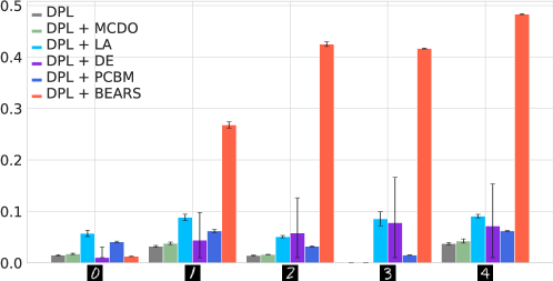
Figure 3: Per-concept entropy shows bears is more uncertain about concepts affected by RS on MNIST-Half compared to regular DPL and alternative uncertainty calibration methods. SL and LTN show similar trends, see Appendix C. Importantly, these improvements do not require concept annotations.

Q1: RSs make NeSy predictors overconfident. Table 1 lists the label and concept ECE of all competitors on MNIST-Half, measured both in-distribution (sums in the training set) and out-of-distribution (all other sums). The label and concept accuracy are reported in the appendix (Table 10) due to space constraints. Overall, all NeSy predictors achieve high label accuracy ($\geq 90\%)$ but fare poorly in terms of concept accuracy (approx. $43\%$ for DPL and SL, and LTN), meaning they are affected by RSs, as expected. Our results also show that they are not RS-aware, as they are very confident about their concept predictions ($\mathrm{ECE}_{C}$ of approx. $69\%$ for DPL, $71\%$ for SL, and $70\%$ fort LTN). Moreover, the label predictions are well calibrated ($\mathrm{ECE}_{Y}$ is approx. $2\%$ for DPL and LTN, $1\%$ for SL), meaning that label uncertainty is not a useful indicator of RSs. In general, models performance worsens out-of-distribution in terms of label accuracy (barely above $0$ for all models) and label and concept calibration (ECE around $90\%$), despite concept accuracy remaining roughly stable (about $40\%$). The results for MNIST-Even-Odd follow a similar trend, cf. Table 11 in the appendix.

As for BDD-OIA , we only evaluate DPL as it is the only model that guarantees predictions comply with the safety constraints out of the ones we consider. The results in Table 2 and Table 12 show that DPL achieves good label accuracy ($72\%$ macro $F_{1}$) in this challenging task by leveraging poor concepts ($34\%$ macro $F_{1}$) with high confidence ($\mathrm{mECE}_{C}\approx 84\%$). This supports our claim that NeSy architectures are not RS-aware.

Q2: Combining NeSy predictors with bears dramatically improves RS-awareness in all data sets while retaining the same prediction accuracy. For MNIST-Half (Table 1, Table 10), bears shrinks the concept ECE from $69\%$ to $37\%$ for DPL, from $71\%$ to $38\%$ for SL, and from $70\%$ to $36\%$ for LTN in-distribution. The out-of-distribution improvement even more substantial, as bears improves both concept calibration (DPL: $87\%\to 38\%$, SL: $88\%\to 37\%$, LTN: $87\%\to 32\%$) and label calibration (DPL: $92\%\to 39\%$, SL: $95\%\to 75\%$, LTN: $94\%\to 36\%$). No competitor comes close. The runner-up, LA, improves concept calibration on average by $10.5\%$ and at best by $15\%$ (for LTN in-distribution), while bears averages $42.3\%$ and up to $55\%$ (for LTN out-of-distribution). Fig. 3 shows that bears correctly assigns high uncertainty to all digits but the zero, which is the only one not affected by RSs, while all competitors are largely overconfident on these digits.

In BDD-OIA the trend is largely the same: bears improves the test set concept ECE for all concepts jointly ($\mathrm{mECE}_{C}$) from $84\%$ to $58\%$ ($-26\%$). The improvement becomes even clearer if we group the various concepts based on what actions they entail: concepts for forward/stop improve by $-61\%$, those for right by $-69\%$, and those for left by $-57\%$. Here, LA performs quite poorly (in fact, it yields worsen calibration), and the runner-up PCBM, which fares well ($-16\%$ $\mathrm{mECE}_{C}$), is also substantially worse than bears. Finally, we note that, despite their similarities, DE underperforms overall, showcasing the importance of our knowledge-aware ensemble diversification strategy.

Q3: bears allows for selecting better concept annotations. Fig. 4 reports the results in terms of concept accuracy on the Kandinsky dataset when using an active learning strategy to acquire concept supervision. Results are obtained by pre-training DPL with 10 examples of red squares, and selecting additional objects for supervision based on their concept uncertainty. Results show that standard DPL has the same behaviour of a random sampling strategy, likely because of its poor estimation of concept uncertainty. On the other hand, DPL with bears manages to substantially outperform both alternatives in improving concept accuracy, achieving an accuracy of more than 90% with just 50 queries, while the other strategies level off at around 75% accuracy. Note that because of the presence of reasoning shortcuts, all models achieve high label-level accuracy regardless of their concept-level accuracy. See Section A.7 for the details.

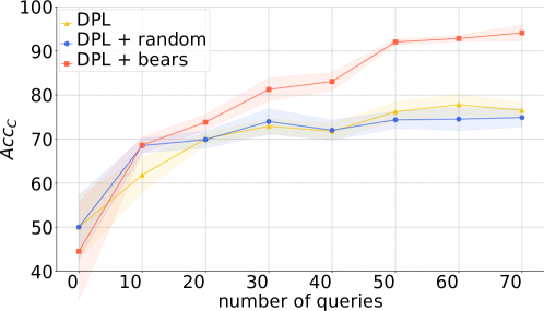
Figure 4: bears allows selecting informative concept annotations faster. A substantial improvement in concept accuracy is achieved by performing active learning guided by RS-aware concept uncertainty (DPL +bears) with respect to plain concept uncertainty (DPL) and random selection.

5 Related Work

Neuro-Symbolic Integration. NeSy AI (Dash et al., 2022; Giunchiglia et al., 2022) spans a broad family of models and tasks – both discriminative and generative – involving perception and reasoning (De Raedt et al., 2021; Garcez et al., 2022; Di Liello et al., 2020; Misino et al., 2022; Ahmed et al., 2023). Given discrete reasoning is not differentiable, NeSy architectures support end-to-end training either by imbuing the prior knowledge with probabilistic (Lippi and Frasconi, 2009; Manhaeve et al., 2018; Yang et al., 2020; Huang et al., 2021; Marra and Kuželka, 2021; Ahmed et al., 2022a; van Krieken et al., 2022a; Skryagin et al., 2022) or fuzzy (Diligenti et al., 2017; van Krieken et al., 2022b; Donadello et al., 2017) semantics, by implementing reasoning in embedding space (Rocktäschel and Riedel, 2016), or through a combination thereof (Pryor et al., 2022). Another difference is whether they encourage (Xu et al., 2018; Fischer et al., 2019; Pryor et al., 2022) vs. guarantee (Manhaeve et al., 2018; Giunchiglia and Lukasiewicz, 2020; Ahmed et al., 2022a; Hoernle et al., 2022; Giunchiglia et al., 2024) predictions to be consistent with the knowledge. Despite their differences, all NeSy approaches can be prone to RSs, which occur whenever prior knowledge – including label supervision – is insufficient to pin down the correct concept semantics.

Dealing with Reasoning Shortcuts. Existing works on RSs focus on unsupervised mitigation, often by discouraging learned concepts from collapsing onto each other. Examples include using a batch-wise entropy loss (Manhaeve et al., 2021), a reconstruction loss (Marconato et al., 2023a), a bottleneck maximization approach (Sansone and Manhaeve, 2023), and encouraging constraint satisfaction via non-trivial assignments (Li et al., 2023). Our work builds on the insights from Marconato et al. (Marconato et al., 2023a), who recently showed that unsupervised mitigation only works in specific cases, and that only expensive strategies – like multi-task learning and dense annotations (Marconato et al., 2023b) – can provably avoid RSs in all cases.

Our key contribution is that of switching focus from mitigation to awareness, which – as we show – can be achieved in an unsupervised manner. In this sense, bears is closely related to unsupervised mitigation heuristics (Manhaeve et al., 2021; Sansone and Manhaeve, 2023; Li et al., 2023), but differs in the goal (awareness vs. mitigation). bears specifically averages over neural networks that capture conflicting RSs to achieve knowledge-dependent uncertainty calibration. It is also related to the neuro-symbolic entropy of (Ahmed et al., 2022b), which, however, minimizes instead of maximizing the entropy of the NeSy predictor, and as such it can exacerbate the negative effects of RSs.

Uncertainty calibration in deep learning. Overconfidence of deep learning models is a well-known issue (Abdar et al., 2021). Many strategies for reducing overconfidence of label predictions exist (Müller et al., 2019; Li et al., 2020; Wei et al., 2022; Mukhoti et al., 2020; Carratino et al., 2022), many of which based on Bayesian techniques (Gal and Ghahramani, 2016; Daxberger et al., 2021; Lakshminarayanan et al., 2017). Our experiments show that applying them to NeSy predictors fails to produce RS-aware models, whereas bears succeeds. Techniques from concept-based models for imbuing concepts with probabilistic semantics (Kim et al., 2023; Marconato et al., 2022; Collins et al., 2023) also can improve calibration, but underperform in our experiments compared to bears.

6 Conclusion

NeSy models tend to be unaware of RSs affecting them, hindering reliability. We address this by introducing bears, which encourages NeSy models to be more uncertain about concepts affected by RSs, enabling users to identify and distrust bad concepts. bears vastly improves RS-awareness compared to NeSy baselines and state-of-the-art calibration methods while retaining high prediction accuracy, and lowers the cost of supervised mitigation via uncertainty-based active learning of dense annotations. In future work, we will explore richer knowledge acquisition strategies to encourage RS-awareness and reduce their impact.

Acknowledgements

The authors are grateful to Zhe Zeng for useful discussion. Funded by the European Union. Views and opinions expressed are however those of the author(s) only and do not necessarily reflect those of the European Union or the European Health and Digital Executive Agency (HaDEA). Neither the European Union nor the granting authority can be held responsible for them. Grant Agreement no. 101120763 - TANGO. AV is supported by the "UNREAL: Unified Reasoning Layer for Trustworthy ML" project (EP/Y023838/1) selected by the ERC and funded by UKRI EPSRC.

Appendix A Implementation Details

In this Section, we provide additional details about all metrics, datasets and models useful for reproducibility.

A.1 Implementation

All the experiments are implemented using Python 3.8 and Pytorch 1.13 and run on one A100 GPU. The implementations of DPL, SL, and LTN were taken verbatim from [Marconato et al., 2023a]. We implemented MCDO and DE by adapting the code to capture the original algorithms [Gal and Ghahramani, 2016, Lakshminarayanan et al., 2017]. For PCBM, we followed the original paper [Kim et al., 2023]. For LA, we adapted the original library from laplace-torch [Daxberger et al., 2021]. In our experiments, we computed the Laplace approximation on the second last layer, mapping the embeddings to the concept layer. The images for Kandinsky patterns were synthetically originated from the resource provided in [Müller and Holzinger, 2021].

A.2 Metrics

For all datasets, we evaluate the predictions on the labels by measuring the accuracy and the $F_{1}$-score with macro average. We assess calibration using the Expected Calibration Error (ECE), which measures how accurately the model-predicted probabilities align with actual data likelihood. Specifically, for a given label $y_{i}\in\mathbb{N}$, the $\mathrm{ECE}_{Y}$ $(i)$ for each label error is evaluated as:

$$\mathrm{ECE}_{Y}(i)=\sum_{\ell=1}^{M}\frac{|B_{\ell}|}{n}|\mathrm{Acc}_{Y}(B_{\ell})-\mathrm{Conf}_{Y}(B_{\ell})|,\quad\forall i\in[m]$$ (9)

where $M$ is the number of bins, $B_{m}$ represent the $m$-th bin and $\mathrm{Conf}_{Y}$ denotes the predicted probability. Essentially, the predicted probabilities are categorized into intervals, denoted as bins. Each data point is assigned to a bin based on its predicted probability. Within each bin, the average predicted probability and accuracy are computed. Ultimately, the ECE value is obtained by summing the averages of absolute differences between predicted probabilities and accuracies. Similarly, we evaluate $\mathrm{ECE}_{C}$ $(j)$ as:

$$\mathrm{ECE}_{C}(j)=\sum_{\ell=1}^{M}\frac{|B_{\ell}|}{n}|\mathrm{Acc}_{C}(B_{\ell})-\mathrm{Conf}_{C}(B_{\ell})|,\quad\forall j\in[k]$$ (10)

In MNIST-Half and MNIST-Even-Odd we use the very same network to extract the first and second digits, and similarly in Kandinsky for extracting the color and shape of each object. For this reason, $\mathrm{ECE}_{C}$ was evaluated by stacking the concepts predicted by the architecture for each object. $\mathrm{ECE}_{Y}$ was evaluated on the final predictions.

In contrast, BDD-OIA images involve multiple concepts and multiple labels. In this case, we adopted a softer approach, specifically we averaged over the performances on each separate component:

$$\mathrm{mECE}_{Y}=\frac{1}{m}\sum_{i=1}^{m}\mathrm{ECE}_{Y}(i)$$ (11)

$$\mathrm{mECE}_{C}=\frac{1}{k}\sum_{i=1}^{k}\mathrm{ECE}_{C}(i)$$ (12)

where $l$ and $k$ are the numbers of labels and concepts, respectively.

In MNIST-Addition and its variations, we evaluate all metrics both in-distribution and out-of-distribution. In Kandinsky, labels and concepts are both balanced, so we report accuracy for both. In BDD-OIA the data is not as balanced, so we report the mean-$F_{1}$, score as in [Sawada and Nakamura, 2022, Marconato et al., 2023a], that is, we first compute the $F_{1}$-score for each action and then average them:

$$\mathrm{mF_{1}}(Y)=\frac{F_{1}(\text{forward})+F_{1}(\text{stop})+F_{1}(\text{left})+F_{1}(\text{right})}{4}$$ (13)

For all datasets, to measure uncertainty concept-wise for a specific model $p_{\theta}$, we rely on the one-vs-all entropy. We evaluate the average entropy of $p_{\theta}(C=c\mid{\bm{\mathrm{x}}})$ as:

$$H_{OVA}(p_{\theta}(C=c|X))=-\frac{1}{|\mathcal{D}|}\sum_{{\bm{\mathrm{x}}}\in\mathcal{D}}\big{[}p_{\theta}(C=c|{\bm{\mathrm{x}}})\log(p_{\theta}(C=c|{\bm{\mathrm{x}}}))+(1-p_{\theta}(C=c|{\bm{\mathrm{x}}}))\log(1-p_{\theta}(C=c|{\bm{\mathrm{x}}}))\big{]}$$ (14)

A.3 bears implementation

Implementation-wise, bears is an extension of DE with a new concept-level repulsive term. In short, bears works as follows. For each new model $\theta_{t}$ to be added to the ensemble, we compute the following loss by considering all other members in ${\bm{\mathrm{\theta}}}=\{\theta_{j}\}_{j=1}^{t-1}$:

$$\max_{\theta_{t}}\frac{1}{|\mathcal{D}|}\sum_{({\bm{\mathrm{x}}},{\bm{\mathrm{y}}})\in\mathcal{D}}\big{[}\log p_{\theta_{t}}({\bm{\mathrm{y}}}\mid{\bm{\mathrm{x}}};\mathsf{K})+\gamma_{1}\mathsf{KL}\big{(}p_{\theta_{t}}({\bm{\mathrm{C}}}\mid{\bm{\mathrm{x}}})\mid\mid\frac{1}{t}\sum_{j=1}^{t}p_{\theta_{j}}({\bm{\mathrm{C}}}\mid{\bm{\mathrm{x}}})\big{)}+\gamma_{2}H(p_{\theta_{t}}({\bm{\mathrm{C}}}\mid{\bm{\mathrm{x}}}))\big{]}$$ (15)

We can analyze further the expression of the $\mathsf{KL}$ divergence to express it differently:

$$\mathsf{KL}\big{(}p_{\theta_{t}}({\bm{\mathrm{C}}}\mid{\bm{\mathrm{x}}})\mid\mid\frac{1}{t}\sum_{j=1}^{t}p_{\theta_{j}}({\bm{\mathrm{C}}}\mid{\bm{\mathrm{x}}})\big{)} =\sum_{{\bm{\mathrm{c}}}\in\{0,1\}^{k}}p_{\theta_{t}}({\bm{\mathrm{c}}}\mid{\bm{\mathrm{x}}})\log\frac{p_{\theta_{t}}({\bm{\mathrm{c}}}\mid{\bm{\mathrm{x}}})}{\frac{1}{t}\sum_{j=1}^{t-1}p_{\theta_{j}}({\bm{\mathrm{c}}}\mid{\bm{\mathrm{x}}})+\frac{1}{t}p_{\theta_{t}}({\bm{\mathrm{c}}}\mid{\bm{\mathrm{x}}})}$$ (16)

$$=-\sum_{{\bm{\mathrm{c}}}\in\{0,1\}^{k}}p_{\theta_{t}}({\bm{\mathrm{c}}}\mid{\bm{\mathrm{x}}})\log\frac{1}{t}\cdot\frac{\sum_{j=1}^{t-1}p_{\theta_{j}}({\bm{\mathrm{c}}}\mid{\bm{\mathrm{x}}})+p_{\theta_{t}}({\bm{\mathrm{c}}}\mid{\bm{\mathrm{x}}})}{p_{\theta_{t}}({\bm{\mathrm{c}}}\mid{\bm{\mathrm{x}}})}$$ (17)

$$=\sum_{{\bm{\mathrm{c}}}\in\{0,1\}^{k}}p_{\theta_{t}}({\bm{\mathrm{c}}}\mid{\bm{\mathrm{x}}})\log{t}-\log\left[1+(t-1)\cdot\sum_{j=1}^{t-1}\frac{1}{t-1}\frac{p_{\theta_{j}}({\bm{\mathrm{c}}}\mid{\bm{\mathrm{x}}})}{p_{\theta_{t}}({\bm{\mathrm{c}}}\mid{\bm{\mathrm{x}}})}\right]$$ (18)

$$=\log{t}-\sum_{{\bm{\mathrm{c}}}\in\{0,1\}^{k}}p_{\theta_{t}}({\bm{\mathrm{c}}}\mid{\bm{\mathrm{x}}})\log\left[1+(t-1)\cdot\frac{p_{rest}({\bm{\mathrm{c}}}\mid{\bm{\mathrm{x}}})}{p_{\theta_{t}}({\bm{\mathrm{c}}}\mid{\bm{\mathrm{x}}})}\right]$$ (19)

where in the second line we introduced a minus sign to flip the term in the logarithm, in the third line we have taken out $p_{\theta_{t}}({\bm{\mathrm{c}}}\mid{\bm{\mathrm{x}}})$ from the numerator and multiplied and divided the remaining terms for $(t-1)$, and in the last line we denoted with $p_{rest}({\bm{\mathrm{c}}}\mid{\bm{\mathrm{x}}})$ the average on the members of the ensemble up to $t-1$.

In general, the $\mathsf{KL}$ divergence is unbounded from above but since the same distribution $p_{\theta_{t}}({\bm{\mathrm{C}}}\mid{\bm{\mathrm{x}}})$ appears from both sides this gives an upper-bound. Notice that, since the $\mathsf{KL}$ is always greater or equal than zero we have that:

$$0\leq\mathsf{KL}\big{(}p_{\theta_{t}}({\bm{\mathrm{C}}}\mid{\bm{\mathrm{x}}})\mid\mid\frac{1}{t}\sum_{j=1}^{t}p_{\theta_{j}}({\bm{\mathrm{C}}}\mid{\bm{\mathrm{x}}})\big{)}\leq\log t$$ (20)

Following, we consider the composite expression with the term proportional to the entropy on the concepts $p_{\theta}({\bm{\mathrm{C}}}\mid{\bm{\mathrm{x}}})$, without accounting for the $\log t$ term. In our implementation, we minimize the term:

$$\min_{\theta}\frac{1}{|\mathcal{D}|}\sum_{({\bm{\mathrm{x}}},{\bm{\mathrm{y}}})\in\mathcal{D}}p_{\theta}({\bm{\mathrm{y}}}\mid{\bm{\mathrm{x}}};\mathsf{K}) +\frac{\gamma_{1}}{\log t}\sum_{{\bm{\mathrm{c}}}\in\{0,1\}^{k}}p_{\theta_{t}}({\bm{\mathrm{c}}}\mid{\bm{\mathrm{x}}})\log\left[1+(t-1)\cdot\frac{p_{rest}({\bm{\mathrm{c}}}\mid{\bm{\mathrm{x}}})}{p_{\theta}({\bm{\mathrm{c}}}\mid{\bm{\mathrm{x}}})}\right]$$ (21)

$$+\gamma_{2}\Big{(}1-\frac{H(p_{\theta_{t}}({\bm{\mathrm{C}}}\mid{\bm{\mathrm{x}}}))}{k\log 2}\Big{)}$$

for each new member of the ensemble, where we divided the $\mathsf{KL}$ term by $\log t$ to ensure its normalization, and we normalized the entropy for the maximal value $k\log 2$. The pseudo-code of bears is shown in Algorithm 1.

Algorithm 1 bears

1:procedure bears($\texttt{n},\texttt{seeds},\gamma_{1},\gamma_{2},\texttt{epochs},\texttt{train\_loader}$)

2:     Initialize empty ensemble 

3:     for $i=1\ldots\texttt{n}$ do

4:         $\texttt{seed}\leftarrow\texttt{seeds}[i]$ # Set seed using $\texttt{seeds}[i]$  

5:         ${\texttt{model}=\tt get\_neq\_model(\texttt{seed})}$ # Create a new ANN model from the seed  

6:         for $e=1,\ldots,\texttt{epochs}$ do

7:              for data $(x,y)$ in train_loader do

8:                  $\hat{y},pcx=\texttt{model}(x)$ # Compute $\hat{y}$ and $p(c\mid x)$  

9:                  $\text{loss}=\text{C}(y,\hat{y})$ # Calculate the loss in classification for the NeSy model  

10:                  if $i>0$ then

11:                       $\overline{pcx}=\text{mean}(pcx)$ # Compute the ensemble average $\overline{p(c|x)}$  

12:                       $\text{loss}=\text{loss}+\gamma_{1}\;\mathsf{KL}(pcx\mid\mid\overline{pcx})+\gamma_{2}\;H(pcx)$ # Update loss with the KL and entropy                     

13:                  loss.backprop() # Backpropagate the loss and update model parameters                          

14:         ensemble$[i]\leftarrow\texttt{model}$ # Add model to ensemble        

15:     return ensemble 

A.4 Datasets details

In our experiments, when possible, we processed different digits and objects with the same neural network. This happens in both MNIST-Addition tasks and Kandinsky, whereas for BDD-OIA this choice is not available.

A.4.1 MNIST-Even-Odd

As done in [Marconato et al., 2023a], we considered the MNIST-Even-Odd dataset, initially introduced in [Marconato et al., 2023b]. This variant of MNIST-Addition has only a few specific combinations of digits, containing either only even or only odd digits:

$$\begin{array}[]{ccc}\begin{cases}\includegraphics[width=7.96527pt]{figures/mnist-0.png}+\includegraphics[width=7.96527pt]{figures/mnist-6.png}&=6\\ \includegraphics[width=7.96527pt]{figures/mnist-2.png}+\includegraphics[width=7.96527pt]{figures/mnist-8.png}&=10\\ \includegraphics[width=7.96527pt]{figures/mnist-4.png}+\includegraphics[width=7.96527pt]{figures/mnist-6.png}&=10\\ \includegraphics[width=7.96527pt]{figures/mnist-4.png}+\includegraphics[width=7.96527pt]{figures/mnist-8.png}&=12\\ \end{cases}&\land&\begin{cases}\includegraphics[width=7.96527pt]{figures/mnist-1.png}+\includegraphics[width=7.96527pt]{figures/mnist-5.png}&=6\\ \includegraphics[width=7.96527pt]{figures/mnist-3.png}+\includegraphics[width=7.96527pt]{figures/mnist-7.png}&=10\\ \includegraphics[width=7.96527pt]{figures/mnist-1.png}+\includegraphics[width=7.96527pt]{figures/mnist-9.png}&=10\\ \includegraphics[width=7.96527pt]{figures/mnist-3.png}+\includegraphics[width=7.96527pt]{figures/mnist-9.png}&=12\\ \end{cases}\end{array}$$ (22)

MNIST-Even-Odd consists of a total of 6720 fully annotated samples in the training set, 1920 samples in the validation set, and 960 samples in the in-distribution test set. Additionally, there are 5040 samples in the out-of-distribution test dataset comprising all other sums that are not observed during training.

Reasoning Shortcuts:

As described in [Marconato et al., 2023a], the number of deterministic RSs can be calculated by finding the integer values for the digits $\includegraphics[width=7.96527pt]{figures/mnist-0.png},\ldots,\includegraphics[width=7.96527pt]{figures/mnist-9.png}$ that solve the above linear system. In total, it was shown that the number of deterministic RSs amounts to 49.

A.4.2 MNIST-Half

This dataset constitutes a biased version of MNIST-Addition, including only half of the digits, specifically, those ranging from $0$ to $4$. Moreover, we selected the following combinations of digits:

$$\begin{cases}\includegraphics[width=7.96527pt]{figures/mnist-0.png}+\includegraphics[width=7.96527pt]{figures/mnist-0.png}&=0\\ \includegraphics[width=7.96527pt]{figures/mnist-0.png}+\includegraphics[width=7.96527pt]{figures/mnist-1.png}&=1\\ \includegraphics[width=7.96527pt]{figures/mnist-2.png}+\includegraphics[width=7.96527pt]{figures/mnist-3.png}&=5\\ \includegraphics[width=7.96527pt]{figures/mnist-2.png}+\includegraphics[width=7.96527pt]{figures/mnist-4.png}&=6\\ \end{cases}$$ (23)

This allows introducing several RSs for the system. Unlike MNIST-Even-Odd, two digits are not affected by reasoning shortcuts: namely $0$ and $1$. The remaining, $2$, $3$, and $4$ can be predicted differently, as shown below.

In total, MNIST-Half comprises 2940 fully annotated samples in the training set, 840 samples in the validation set, 420 samples in the test set, and an additional 1080 samples in the out-of-distribution test dataset. These only comprise the remaining sums with these digits, like $\includegraphics[width=7.96527pt]{figures/mnist-1.png}+\includegraphics[width=7.96527pt]{figures/mnist-3.png}=4$.

Reasoning shortcuts:

We identify all the possible RSs empirically, since the system of observed sums can be written as a linear system from Eq. 23. There are in total three possible optimal solutions, of which two are reasoning shortcuts. Explicitly:

$$\includegraphics[width=7.96527pt]{figures/mnist-0.png}\mapsto 0,\ \includegraphics[width=7.96527pt]{figures/mnist-1.png}\mapsto 1, \includegraphics[width=7.96527pt]{figures/mnist-2.png}\mapsto 2,\ \includegraphics[width=7.96527pt]{figures/mnist-3.png}\mapsto 3,\ \includegraphics[width=7.96527pt]{figures/mnist-4.png}\mapsto 4$$ (24)

$$\lor$$

$$\includegraphics[width=7.96527pt]{figures/mnist-0.png}\mapsto 0,\ \includegraphics[width=7.96527pt]{figures/mnist-1.png}\mapsto 1, \includegraphics[width=7.96527pt]{figures/mnist-2.png}\mapsto 3,\ \includegraphics[width=7.96527pt]{figures/mnist-3.png}\mapsto 2,\ \includegraphics[width=7.96527pt]{figures/mnist-4.png}\mapsto 3,$$

$$\lor$$

$$\includegraphics[width=7.96527pt]{figures/mnist-0.png}\mapsto 0,\ \includegraphics[width=7.96527pt]{figures/mnist-1.png}\mapsto 1, \includegraphics[width=7.96527pt]{figures/mnist-2.png}\mapsto 4,\ \includegraphics[width=7.96527pt]{figures/mnist-3.png}\mapsto 1,\ \includegraphics[width=7.96527pt]{figures/mnist-4.png}\mapsto 2,$$

A.4.3 Kandinsky

This dataset, introduced in [Müller and Holzinger, 2021], consists of visual patterns inspired by the artistic works of Wassily Kandinsky. These patterns are made of geometric figures, with several features. In our experiment, we propose a variant of Kandinsky where each image has a fixed number of figures, and the associated concepts are shape and color. In total, each object can take one among three possible colors $(\tt red,blue,yellow)$ and one among three possible shapes $(\tt square,circle,triangle)$.

We propose our Kandinsky variant for an active learning setup resembling an IQ test for machines. The task is to predict the pattern of a third image given two images sharing a common pattern. The example below provides an idea of this task.

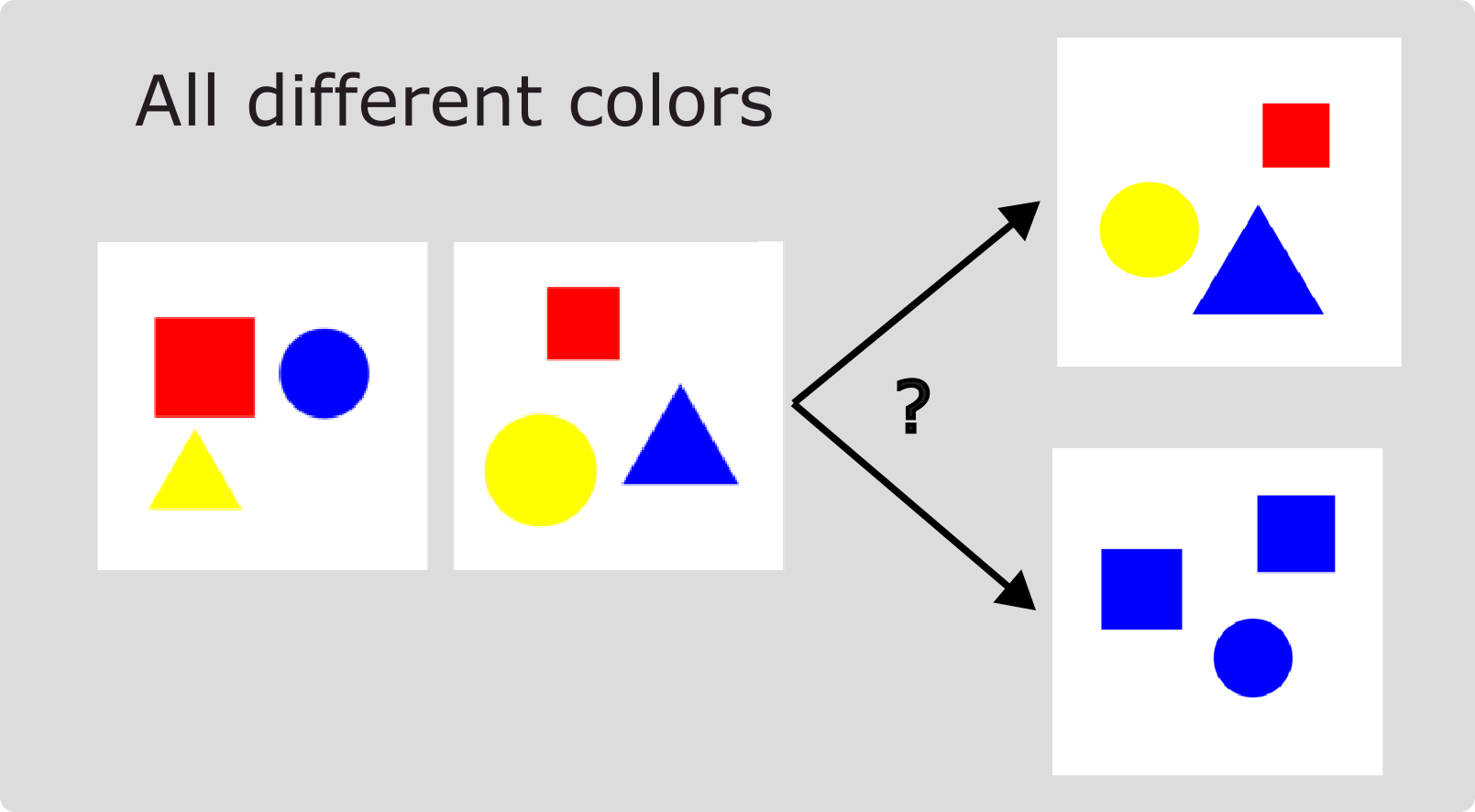
Figure 5: An example of a test sample for the Kandinsky task. At inference time, the NeSy model has to choose according to the previous two images the third that completes the pattern. For each image, the model computes a series of predicates, like same_cs, same_ss, and so on. In this case, the first two images have different colors, so the model should pick the first option.

Formally, let $x$ be an object in the figure, $S(x)$ the shape of $x$, and $C(x)$ its color. Let the image be denoted as $Figure$. In total, each figure contains three objects with possibly different colors and shapes. To enhance the clarity and conciseness of our logical expressions, we introduce the following shorthand predicates:

$$\begin{cases}&\text{{diff\_s}}(Figure)\equiv\forall x,y\in Figure:\left(x\neq y\rightarrow\neg\left(S(x)=S(y)\right)\right)\\ &\text{{diff\_c}}(Figure)\equiv\forall x,y\in Figure:\left(x\neq y\rightarrow\neg\left(C(x)=C(y)\right)\right)\\ &\text{{same\_s}}(Figure)\equiv\forall x,y\in Figure:\left(S(x)=S(y)\right)\\ &\text{{same\_c}}(Figure)\equiv\forall x,y\in Figure:\left(C(x)=C(y)\right)\\ &\text{{pair\_c}}(Figure)\equiv\neg\text{{same\_c}}(Figure)\land\neg\text{{diff\_c}}(Figure)\\ &\text{{pair\_s}}(Figure)\equiv\neg\text{{same\_s}}(Figure)\land\neg\text{{diff\_s}}(Figure)\\ \end{cases}$$ (25)

Let $Sample$ represent a training sample consisting of two figures for the sake of simplicity; the extension to more figures is trivial. The final logic statement, that determines the model output, is:

$$\text{{shared\_pattern}}\Rightarrow\forall f_{1},f_{2}\in\textit{Sample}:$$ (26)

$$(\texttt{same\_c}(f_{1})\land\texttt{same\_c}(f_{2}))\lor(\texttt{pair\_c}(f_{1})\land\texttt{pair\_c}(f_{2}))\lor(\texttt{diff\_c}(f_{1})\land\texttt{diff\_c}(f_{2}))$$

$$\hskip 200.0003pt\lor$$

$$(\texttt{same\_s}(f_{1})\land\texttt{same\_s}(f_{2}))\lor(\texttt{pair\_s}(f_{1})\land\texttt{pair\_s}(f_{2}))\lor(\texttt{diff\_s}(f_{1})\land\texttt{diff\_s}(f_{2}))$$

Our Kandinsky dataset version comprises $4$k examples in training, $1$k in validation, and $1$k in test.

We create our dataset to include a balanced number of positive and negative examples. Positive examples consist of three images sharing the same pattern, while in negative examples the third image does not match the pattern which is shared by the first two images. The order of examples does not introduce bias into the neural network learning procedure, as the network treats each figure independently.

Preprocessing:

When processing an entire figure at once, we empirically observed that the model faces challenges in achieving satisfactory accuracy. Consequently, we opted to process one object at a time. Therefore, we employed a simplified version of the dataset that comprises of rescaled objects manually extracted via bounding boxes. Thus, each example of the dataset consists of 9 objects, namely 3 objects for each figure, ordered based on their distance from the origin of the figure.

Reasoning shortcuts:

The knowledge we build for Kandinsky admits many RSs. As there are no constraints on specific colors or shapes, in principle, each permutation of colors and shapes can achieve perfect accuracy. Furthermore, the logic is symmetrical; hence, the concepts of colors and shapes could be swapped. Working on this dataset, we have observed various RSs. An example is illustrated below:

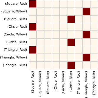
Figure 6: This plot shows an example of a RS in the Kandinsky task. The model achieves perfect accuracy by predicting shapes based on their colors. In this scenario, all red objects are correctly identified as squares, blue ones as circles, and yellow ones as triangles.

A.4.4 BDD-OIA

This dataset is made of frames retrieved from driving scene videos for autonomous driving predictions [Xu et al., 2020]. Each frame is labeled with four binary actions (move_forward, stop, turn_left, turn_right). Scenes are annotated with $21$ binary concepts, providing explanations for the chosen actions. The training set includes $16$k fully labeled frames, while the validation and test sets have $2$k and $4.5$k annotated data, respectively.

The prior knowledge employed is the same as in [Marconato et al., 2023a]. We report it here for the sake of completeness. For the move_forward and stop move, the rules are:

$$\begin{cases}&\text{{red\_light}}\Rightarrow\lnot\text{{green\_light}}\\ &\text{{obstacle}}=\text{{car}}\lor\text{{person}}\lor\text{{rider}}\lor\text{{other\_obstacle}}\\ &\text{{road\_clear}}\Longleftrightarrow\lnot\text{{obstacle}}\\ &\text{{green\_light}}\lor\text{{follow}}\lor\text{{clear}}\Rightarrow\text{{move\_forward}}\\ &\text{{red\_light}}\lor\text{{stop\_sign}}\lor\text{{obstacle}}\Rightarrow\text{{stop}}\\ &\text{{stop}}\Rightarrow\lnot\text{{move\_forward}}\\ \end{cases}$$ (27)

While for the turn_left and the turn_right action, the rules are:

$$\begin{cases}&\text{{can\_turn}}=\text{{left\_lane}}\lor\text{{left\_green\_lane}}\lor\text{{left\_follow}}\\ &\text{{cannot\_turn}}=\text{{no\_left\_lane}}\lor\text{{left\_obstacle}}\lor\text{{left\_solid\_line}}\\ &\text{{can\_turn}}\land\lnot\text{{cannot\_turn}}\Rightarrow\text{{turn\_left}}\\ \end{cases}$$ (28)

Moreover, for convenience in metric computations, we decided to group the actions into three classes of concepts. Specifically, we define $F-S$, which groups concepts concerning the move_forward and stop actions, $L$, which groups concepts concerning the turn_left action, and the $R$ group, which denotes the actions concerning the turn_right action. The classes are shown in Table 3.

Concept Class	Concepts
$F-S$	green_light
	follow
	road_clear
	red_light
	traffic_sign
	car
	person
	rider
	other_obstacle
$L$	left_lane
	left_green_light
	left_follow
	no_left_lane
	left_obstacle
	letf_solid_line
$R$	right_lane
	right_green_light
	right_follow
	no_right_lane
	right_obstacle
	right_solid_line

Table 3: Concept classes in BDD-OIA

A.5 Hyperparameters and Model selection

In our work, we opted for the widely used Adam optimizer [Kingma and Ba, 2015]. For MNIST-Half and MNIST-Even-Odd, the learning rate follows an exponential decay with $\gamma=0.95$. Regarding BDD-OIA , the weight decay is $\omega=1\cdot 10^{-3}$ for all DPL variants, except for PCBM where we set it to $0.01$. For the learning rate $\gamma$, it is set to $0.2$ for DPL and its variants. However, we observed that a $\gamma=1$ works best for PCBM since this model does not converge very early. In the active learning experiment on Kandinsky, we applied exponential decay with $\gamma=0.9$.

To choose the hyperparameters, we conducted a grid search over a predefined set of values, and selected the best values based on both qualitative and quantitative results from a validation set. The learning rate for all experiments was fine-tuned within the range of $10^{-4}$ to $10^{-2}$. Specifically, for MNIST-Half, we set the learning rate to $5\cdot 10^{-4}$ for DPL, and $1\cdot 10^{-3}$ for SL, LTN, and PCBM. For Kandinsky, the learning rate was set to $1\cdot 10^{-3}$. In the case of BDD-OIA , we explored a learning rate range between $10^{-4}$ and $10^{-2}$ and selected $10^{-3}$ for all the models.

Regarding batch sizes, we observed that $64$ worked well for MNIST-Even-Odd and MNIST-Half, and $512$ for BDD-OIA . For Kandinsky, a smaller batch size of $16$ was chosen as more frequent updates helped with model convergence.

Empirically, for bears, we discovered that optimizing $\gamma_{1}$ and $\gamma_{2}$ significantly influenced ensemble diversity, leading to different outcomes. Specifically, when these hyperparameters are much lower compared to the classification loss, the ensemble models tend to converge toward a single reasoning shortcut, reducing the impact of bears. Conversely, if these hyperparameters are bigger, the ensemble may consist of entirely different solutions, but potentially sub-optimal ones. These hyperparameters should be carefully tuned to strike a balance. We performed a grid search for both parameters over $\eta=\{0.1,0.8,0.5,1,2,5,10\}$ and selected the best values based on minimizing the classification objective and maximizing ensemble diversity.

For MNIST-Half and MNIST-Even-Odd, we observed that the impact of entropy is negligible. Consequently, we set $\gamma_{2}=0$ for all experiments. In contrast, relying solely on the $\mathsf{KL}$ term in BDD-OIA and Kandinsky does not effectively explore a consistent space of reasoning shortcuts. Thus, for bears, we set $\gamma_{1}=0.1$ for LTN and $\gamma_{1}=5$ for SL. For DPL, we set $\gamma_{1}=0.8$ for MNIST-Half and MNIST-Even-Odd, $\gamma_{1}=0.1$ and $\gamma_{2}=1$ for BDD-OIA , and $\gamma_{1}=0.01$ for Kandinsky.

Concerning the number of ensembles, a shared hyperparameter for DE and bears, we chose $5$ for MNIST-Half, MNIST-Even-Odd, and Kandinsky, and $20$ for BDD-OIA , considering the larger number of reasoning shortcuts in the latter. In BDD-OIA there $7^{21}\cdot 57^{114}\cdot 280^{280}$, compared to the $49$ present in MNIST-Even-Odd Marconato et al. [2023a].

Additionally, we observed that LTN behavior is quite unstable, resulting in sub-optimal models regardless of hyperparameter choices. To address this, we introduced an entropy penalization of $0.3$ to aid model convergence. The same approach was applied to DPL on Kandinsky, where this value was set to $0.2$.

Regarding the number of LA sampling and MCDO, we observed no big difference, thus we selected $30$ for our experiments.

Specifically for LA, we applied the Laplace approximation to the concept layer of the pre-trained frequentist model. For MNIST-Half and MNIST-Even-Odd, we used the Kronecker approximation of the Hessian matrix, but we could not use it for BDD-OIA due to excessive time and memory requirements. For BDD-OIA , we switched to the diagonal approximation.

For PCBM, the optimization involves the sum of two losses: a cross-entropy loss and a concept loss. The concept loss, denoted as $\mathcal{L}_{\text{concept}}$, is defined as $\mathcal{L}_{\text{concept}}=\mathcal{L}_{BCE}+\lambda_{\text{KL}}\mathcal{L}_{KL}$ [Kim et al., 2023]. Here, $\mathcal{L}_{BCE}$ represents the standard binary cross-entropy, and $\mathcal{L}_{KL}$ serves as a regularization term for the Gaussian distribution, defined as $\mathcal{L}_{KL}=\mathsf{KL}(N(\mu_{c},\text{diag}(\sigma_{c}))||N(0,I))$. Since we lack concept supervision during training, the weight associated with the binary cross-entropy is set to $0$. The regularization term $\lambda_{kl}$ is maintained at $0.001$ for both examples, as setting it too high led to sub-optimal models in our specific context.

Finally, concerning the active learning example on Kandinsky, we found that to achieve optimal convergence while still learning concepts, effective parameters for the concept supervision loss are $25$ for DPL and $10$ for DPL + bears.

A.6 Architectures and Model Details

MNIST-Addition:

The architectures employed for MNIST-Even-Odd and MNIST-Half are essentially the one implemented in [Marconato et al., 2023a], outlined in Table 4. The only difference among the two datasets is the size of the bottleneck, which depends on the number of concepts. For MNIST-Half, the last layer dimension is 10, while for MNIST-Even-Odd is 20. For PCBM, the architecture is shown in Table 6. Additionally, for SL only, we introduced an MLP with a hidden size of 50 neurons. This MLP takes the logits of both concepts as input and processes them to produce the final label.

Table 4: Encoder architecture for MNIST-Half, MNIST-Even-Odd.

Input	Layer Type	Parameter	Activation
$(28,56,1)$	Convolution	depth=32, kernel=4, stride=2, padding=1	ReLU
$(32,14,28)$	Dropout	$p=0.5$
$(32,14,28)$	Convolution	depth=64, kernel=4, stride=2, padding=1	ReLU
$(64,7,14)$	Dropout	$p=0.5$
$(64,7,14)$	Convolution	depth=$128$, kernel=4, stride=2, padding=1	ReLU
$(128,3,7)$	Flatten
$(2688)$	Linear	dim=20, bias = True

Table 5: Encoder architecture for Kandinsky

Input	Layer Type	Parameter	Activation
$(28,28,3)$	Flatten
$(2352)$	Linear	dim=256, bias=True	ReLU
$(256)$	Dropout	$p=0.5$
$(256)$	Linear	dim=128, bias=True	ReLU
$(128)$	Dropout	$p=0.5$
$(128)$	Linear	dim=8, bias = True

Table 6: Encoder architecture for PCBM

Input	Layer Type	Parameter	Activation	Note
$(28,56,1)$	Convolution	depth=32, kernel=4, stride=2, padding=1	ReLU
$(32,14,28)$	Dropout	$p=0.5$
$(32,14,28)$	Convolution	depth=64, kernel=4, stride=2, padding=1	ReLU
$(64,7,14)$	Dropout	$p=0.5$
$(64,7,14)$	Convolution	depth=$128$, kernel=4, stride=2, padding=1	ReLU
$(128,3,7)$	Flatten
$(2688)$	Linear	dim=160, bias = True		Head for $\mu$
$(2688)$	Linear	dim=160, bias = True		Head for $\sigma$

BDD-OIA :

Likewise for [Marconato et al., 2023a], BDD-OIA images have been preprocessed, as detailed in [Sawada and Nakamura, 2022], employing a Faster-RCNN [Ren et al., 2015] pre-trained on MS-COCO and fine-tuned on BDD-100k, for initial preprocessing. Subsequently, we employ a pre-trained convolutional layer from [Sawada and Nakamura, 2022] to extract linear features with a dimensionality of 2048. These linear features serve as inputs for the NeSy model, implemented with a fully-connected classifier network as outlined in Table 7 for DPL, and in Table 8 for PCBM.

Kandinsky:

For Kandinsky, we chose to use an MLP-based encoder, as depicted in Table 5.

Table 7: DPL architecture for BDD-OIA

Input	Layer Type	Parameter	Activation	Note
$(2048,1)$	Linear	dim=512, bias=True	ReLU
$(512)$	Dropout
$(512)$	Linear	dim=21, bias=True		Head for move_forward action
$(512)$	Linear	dim=12, bias=True		Head for stop action
$(512)$	Linear	dim=12, bias=True		Head for turn_left action
$(512)$	Linear	dim=12, bias=True		Head for turn_right action

Table 8: PCBM architecture for BDD-OIA

Input	Layer Type	Parameter	Activation	Note
$(2048,1)$	Linear	dim=336, bias=True		Head for $\mu$
$(2048,1)$	Linear	dim=336, bias=True		Head for $\sigma$

A.7 Active Learning Setup

The active learning setup proposed is based on Kandinsky. The examples consist of three figures, each composed of three objects. Each object is characterized by shape and color properties. In this setup, the model processes each object independently, producing a 6-dimensional vector that includes the one-hot encoding of shapes and colors, with each dimension representing one of the three shapes or colors. Overall, for each figure the model produces an 18-dimensional vector. The supervision is provided for a single object and consists of its shape and color.

To configure the experiment, we masked all the concepts in the training set, revealing them only when the object is chosen for supervision. Therefore, the active learning setup does not involve adding new examples to the training set but rather unveiling concepts in the existing ones.

The model was initialized by providing supervision on 10 red-squares, that was sufficient to allow it to achieve optimal accuracy (by learning a reasoning shortcut). Notice that without any initial concept-level supervision, the model was incapable of achieving decent accuracy results because of the complexity of the knowledge.

At each step of the active learning setup, both DPL and bears compute the Shannon entropy on an object, defined as:

$$H(\mathbf{s},\mathbf{c}|x)=-\sum_{i,j}p_{\theta}(s_{i},c_{j}|x)\log p_{\theta}(s_{i},c_{j}|x)$$ (29)

where $p_{\theta}(s_{i},c_{j}|x)$ is the probability of shape $s_{i}$ and color $c_{j}$ for object $x$. Plain DPL computes the probability of a certain configuration of concepts for an object $x$ as:

$$p_{\theta}(s_{i},c_{j}|x)=p_{\theta}(s_{i}|x)p_{\theta}(c_{j}|x)$$ (30)

while bears computes it as:

$$p_{{\bm{\mathrm{\theta}}}}(s_{i},c_{j}|x)=\cfrac{1}{|{\bm{\mathrm{\theta}}}|}\sum_{\theta^{\prime}\in{\bm{\mathrm{\theta}}}}p_{\theta^{\prime}}(s_{i}|x)p_{\theta^{\prime}}(c_{j}|x)$$ (31)

Where ${\bm{\mathrm{\theta}}}$ is the learned ensemble. The top 10 elements with largest entropy are then selected to acquire concept-level supervision. The baseline method DPL + random ignores concept uncertainty altogether and simply chooses 10 random elements from the training set.

A.8 Runtime Comparison

Table 9: Wall-clock time for a single batch in MNIST-Half

Method	Train - batch	Inference - batch	Pre-process
DPL	$0.011$	$0.001$
DPL + MCDO		$0.026$
DPL + LA		$0.019$	$32.249$
DPL + PCBM	$0.043$	$0.043$
DPL + DE	$0.017$	$0.027$
DPL + bears	$0.073$	$0.018$
SL	$0.010$	$0.001$
SL + MCDO		$0.017$
SL + LA		$0.013$	$21.990$
SL + PCBM	$0.043$	$0.054$
SL + DE	$0.033$	$0.020$
SL + bears	$0.085$	$0.014$
LTN	$0.010$	$0.001$
LTN + MCDO		$0.018$
LTN + LA		$0.014$	$26.434$
LTN + PCBM	$0.035$	$0.045$
LTN + DE	$0.031$	$0.017$
LTN + bears	$0.072$	$0.011$

To estimate the order of magnitude of bears, we measured the wall-clock time of a run on MNIST-Half. Specifically, we computed the wall-clock time of the model inference on a single batch (all batches have the same dimension, i.e. $64$). For both DE and bears, we evaluated only a single model of the ensemble, namely the last model out of $5$. In this way, we isolate the time from the number of ensembles. We do not report the training time for MCDO and LA as they are applied on pre-trained models. Additionally, we account for the pre-processing time of LA, which is needed to compute the Hessian matrix for the Laplace approximation. However, it is important to note that this step is done only once.

As shown in Table 9, the inference time of bears is comparable to all the competitors, as long as the ensemble is not too big. In terms of training, although we take more time due to the overhead associated with the retrieval of the $p(C|x)$ for ensemble members and the computation of the loss function, we are comparable with DE.

Appendix B Theoretical Material

In this section, we include the proofs and the theoretical material needed for the main text. Before moving to the proofs of the main text claims, we report the statement of Lemma 1, Theorem 2, and Proposition 3 from [Marconato et al., 2023a] for ease of comparison. These rely on two assumptions, cf. Section 3:

• Invertibility: Each ${\bm{\mathrm{x}}}$ is generated by a unique ${\bm{\mathrm{g}}}$, i.e., there exists a function $f:{\bm{\mathrm{x}}}\mapsto{\bm{\mathrm{g}}}$ such that $p^{*}({\bm{\mathrm{G}}}\mid{\bm{\mathrm{X}}})=\mathbbm{1}\!\left\{{\bm{\mathrm{G}}}-f({\bm{\mathrm{X}}})\right\}$.

• Determinism: The knowledge $\mathsf{K}$ is deterministic, i.e., there exists a function $\beta_{\mathsf{K}}:{\bm{\mathrm{g}}}\mapsto{\bm{\mathrm{y}}}$ such that $p^{*}({\bm{\mathrm{Y}}}\mid{\bm{\mathrm{G}}};\mathsf{K})=\mathbbm{1}\!\left\{{\bm{\mathrm{Y}}}=\beta_{\mathsf{K}}({\bm{\mathrm{g}}})\right\}$.

We begin by reporting three useful results from [Marconato et al., 2023a] that will be used in our proofs. First of all, we will indicate with $\mathsf{supp}({\bm{\mathrm{G}}})$ the support of the probability distribution given by $p^{*}({\bm{\mathrm{G}}})$.

Lemma 4.

It holds that: (ii) Under A1, there exists a bijection between the deterministic concept distributions $p_{\theta}({\bm{\mathrm{C}}}\mid{\bm{\mathrm{X}}})$ that are constant over the support of $p({\bm{\mathrm{X}}}\mid{\bm{\mathrm{g}}})$, for each ${\bm{\mathrm{g}}}\in\mathrm{supp}({\bm{\mathrm{G}}})$, and the deterministic distributions of the form $p_{\theta}({\bm{\mathrm{C}}}\mid{\bm{\mathrm{G}}})$.

Theorem 5.

Let $\mathcal{A}$ be the set of mappings $\alpha:{\bm{\mathrm{g}}}\mapsto{\bm{\mathrm{c}}}$ induced by all possible deterministic distributions $p_{\theta}({\bm{\mathrm{C}}}\mid{\bm{\mathrm{G}}})$, i.e., each $p_{\theta}({\bm{\mathrm{C}}}\mid{\bm{\mathrm{G}}})=\mathbbm{1}\!\left\{{\bm{\mathrm{C}}}=\alpha({\bm{\mathrm{G}}})\right\}$ for exactly one $\alpha\in\mathcal{A}$. Under A1 and A2, the number of deterministic optima $p_{\theta}({\bm{\mathrm{C}}}\mid{\bm{\mathrm{G}}})$ is:

$$\textstyle\sum_{\alpha\in\mathcal{A}}\mathbbm{1}\!\left\{\bigwedge_{{\bm{\mathrm{g}}}\in\mathsf{supp}({\bm{\mathrm{G}}})}(\beta_{\mathsf{K}}\circ\alpha)({\bm{\mathrm{g}}})=\beta_{\mathsf{K}}({\bm{\mathrm{g}}})\right\}$$ (32)

In particular, the set of optimal maps $\mathcal{A}^{*}$ is given by:

$$\textstyle\mathcal{A}^{*}=\big{\{}\alpha\in\mathcal{A}:\;\bigwedge_{{\bm{\mathrm{g}}}\in\mathsf{supp}({\bm{\mathrm{G}}})}(\beta_{\mathsf{K}}\circ\alpha)({\bm{\mathrm{g}}})=\beta_{\mathsf{K}}({\bm{\mathrm{g}}})\big{\}}$$ (33)

Proposition 6.

For probabilistic logic approaches (including DPL and SL): (i) All convex combinations of two or more deterministic optima $p_{\theta}({\bm{\mathrm{C}}}\mid{\bm{\mathrm{X}}})$ of the likelihood are also (non-deterministic) optima. However, not all convex combinations can be expressed in DPL and SL. (ii) Under A1 and A2, all optima of the likelihood can be expressed as a convex combination of deterministic optima. (iii) If A2 does not hold, there may exist non-deterministic optima that are not convex combinations of deterministic ones. These may be the only optima.

B.1 Proof of Lemma 1

Lemma.

Take any input-concept distribution $p({\bm{\mathrm{C}}}\mid{\bm{\mathrm{X}}})$ and let $p({\bm{\mathrm{C}}}\mid{\bm{\mathrm{G}}})$ be the concept-concept distribution entailed by it. Then there exists (at least one) vector ${\bm{\mathrm{\omega}}}$ such that $p$ is a convex combination of maps $\alpha\in\mathcal{A}$, that is:

$$p({\bm{\mathrm{C}}}\mid{\bm{\mathrm{G}}})=\sum_{\alpha\in\mathcal{A}}\omega_{\alpha}\mathbbm{1}\!\left\{{\bm{\mathrm{C}}}=\alpha({\bm{\mathrm{G}}})\right\}:=p_{\omega}({\bm{\mathrm{C}}}\mid{\bm{\mathrm{G}}})$$

parameterized by ${\bm{\mathrm{\omega}}}\geq 0$, $\lVert{\bm{\mathrm{\omega}}}\rVert_{1}=1$. Moreover, under invertibility (A1) and determinism (A2), the set of all maps $\mathcal{A}$ restricts to the set of optimal maps $\mathcal{A}^{*}$.

Proof.

By definition, $p({\bm{\mathrm{C}}}\mid{\bm{\mathrm{G}}})$ is given by:

$$p({\bm{\mathrm{C}}}\mid{\bm{\mathrm{G}}}):=\mathbb{E}_{p({\bm{\mathrm{x}}}\mid{\bm{\mathrm{g}}})}p({\bm{\mathrm{C}}}\mid{\bm{\mathrm{x}}})$$ (34)

For each ${\bm{\mathrm{g}}}\in\{0,1\}^{k}$, $p({\bm{\mathrm{C}}}\mid{\bm{\mathrm{g}}})$ can be written as a convex combination of the maps $\alpha\in\mathcal{A}$:

$$p({\bm{\mathrm{C}}}\mid{\bm{\mathrm{g}}}) =\sum_{{\bm{\mathrm{c}}}}p({\bm{\mathrm{c}}}\mid{\bm{\mathrm{g}}})\mathbbm{1}\!\left\{{\bm{\mathrm{C}}}={\bm{\mathrm{c}}}\right\}$$ (35)

$$=\sum_{\bm{\mathrm{c}}}\left[\sum_{\alpha\in\mathcal{A}}\omega_{\alpha}\mathbbm{1}\!\left\{\alpha({\bm{\mathrm{g}}})={\bm{\mathrm{c}}}\right\}\right]\mathbbm{1}\!\left\{{\bm{\mathrm{C}}}={\bm{\mathrm{c}}}\right\}$$

$$=\sum_{\alpha\in\mathcal{A}}\omega_{\alpha}\mathbbm{1}\!\left\{{\bm{\mathrm{C}}}=\alpha({\bm{\mathrm{g}}})\right\}$$

where in the last line we swapped the summation and used the condition that $\alpha({\bm{\mathrm{g}}})={\bm{\mathrm{c}}}$. Altogether, this yields for the single ${\bm{\mathrm{g}}}$ that the following must hold:

$$\sum_{\alpha\in\mathcal{A}:\,\alpha({\bm{\mathrm{g}}})={\bm{\mathrm{c}}}}\omega_{\alpha}=p({\bm{\mathrm{c}}}\mid{\bm{\mathrm{g}}})$$ (36)

Combining all the cases this gives a system of $2^{k}\cdot{2^{k}}$ equations, one for each ${\bm{\mathrm{g}}}$ and for each ${\bm{\mathrm{c}}}$, for a total of $(2^{k})^{2^{k}}$ variables ${\bm{\mathrm{\omega}}}$:

$$\sum_{\alpha\in\mathcal{A}:\,\alpha({\bm{\mathrm{g}}})={\bm{\mathrm{c}}}}\omega_{\alpha}=p({\bm{\mathrm{c}}}\mid{\bm{\mathrm{g}}}),\quad\forall{\bm{\mathrm{g}}}\in\{0,1\}^{k},\;\forall{\bm{\mathrm{c}}}\in\{0,1\}^{k}$$ (37)

This shows that the linear system can always be solved, proving that $\mathcal{A}$ spans the space of $p({\bm{\mathrm{C}}}\mid{\bm{\mathrm{G}}})$.

Next, under A1 and A2 we have that to have an optimal model we only need to consider the optimal elements $\alpha\in\mathcal{A}^{*}$, where the set $\mathcal{A}^{*}$ is defined from Theorem 5:

$$\textstyle\mathcal{A}^{*}=\big{\{}\alpha\in\mathcal{A}:\;\bigwedge_{{\bm{\mathrm{g}}}\in\mathrm{supp}({\bm{\mathrm{G}}})}(\beta_{\mathsf{K}}\circ\alpha)({\bm{\mathrm{g}}})=\beta_{\mathsf{K}}({\bm{\mathrm{g}}})\big{\}}$$ (38)

We proceed by contradiction. Suppose there exists one $\alpha^{\prime}\not\in\mathcal{A}^{*}$ such that:

$$p({\bm{\mathrm{C}}}\mid{\bm{\mathrm{G}}})=\omega(\alpha^{\prime})\mathbbm{1}\!\left\{{\bm{\mathrm{C}}}=\alpha^{\prime}({\bm{\mathrm{g}}})\right\}+\sum_{\alpha\in\mathcal{A}^{*}}\omega_{\alpha}\mathbbm{1}\!\left\{{\bm{\mathrm{C}}}=\alpha({\bm{\mathrm{g}}})\right\}$$ (39)

is still optimal. Notice that there exists at least one ${\bm{\mathrm{g}}}$ such that $\alpha^{\prime}({\bm{\mathrm{g}}})\neq\alpha({\bm{\mathrm{g}}})$, $\forall\alpha\in\mathcal{A}^{*}$. This means that for those values ${\bm{\mathrm{g}}}$ we have $(\beta_{\mathsf{K}}\circ\alpha^{\prime})({\bm{\mathrm{g}}})\neq\beta_{\mathsf{K}}({\bm{\mathrm{g}}})$. Therefore, the NeSy predictor will result in a suboptimal model, since it does not place the mass on concepts attaining the same label. This proves the contradiction, yielding the claim. ∎

B.2 Entropy on concept vectors and Reasoning Shortcuts

Under invertibility (A1) and determinism (A2), it is possible to describe entirely the set of optimal maps $\alpha:{\bm{\mathrm{G}}}\mapsto{\bm{\mathrm{C}}}$ through Theorem 5, which we denote with $\mathcal{A}^{*}$. Before moving on to prove the main results in the main text, it is useful to introduce here the notion of “equivalence set” of a concept vector ${\bm{\mathrm{g}}}$ given the optimal maps $\alpha\in\mathcal{A}^{*}$:

$$\mathcal{E}({\bm{\mathrm{g}}};\mathsf{K})=\{\alpha({\bm{\mathrm{g}}}):\;\forall\alpha\in\mathcal{A}^{*}\}$$ (40)

that contains all the concepts ${\bm{\mathrm{c}}}\in\{0,1\}^{k}$ that are predicted by the maps $\alpha\in\mathcal{A}^{*}$. With this, we can formally define when a ground-truth concept ${\bm{\mathrm{g}}}$ is mispredicted by RSs:

Definition 1.

We say that a concept vector ${\bm{\mathrm{g}}}\in\{0,1\}^{k}$ is “mispredicted” by RSs when $|\mathcal{E}({\bm{\mathrm{g}}};\mathsf{K})|>1$, i.e., there exist at least two different $\alpha_{i},\alpha_{j}\in\mathcal{A}^{*}$, such that $\alpha_{i}({\bm{\mathrm{g}}})\neq\alpha_{j}({\bm{\mathrm{g}}})$. Conversely, a concept vector is “correctly predicted” if $\alpha({\bm{\mathrm{g}}})={\bm{\mathrm{g}}}$, $\forall\alpha\in\mathcal{A}^{*}$.

Following, we can use the decomposition in terms of the map $\alpha$’s to inspect what combinations with optimal weights ${\bm{\mathrm{\omega}}}^{*}=(\omega_{1},\ldots,\omega_{N})$, where $N=|\mathcal{A}^{*}|$ and $\lVert{\bm{\mathrm{\omega}}}^{*}\rVert_{1}=1$, give high entropy on single concepts ${\bm{\mathrm{g}}}\in\{0,1\}^{k}$:

Proposition 7.

Suppose that $p_{\bm{\mathrm{\omega}}}({\bm{\mathrm{C}}}\mid{\bm{\mathrm{G}}})$ admits a decomposition as a weighted sum of at least two distinct $\alpha\in\mathcal{A}$, with weights ${\bm{\mathrm{\omega}}}$. Then,

• for any ${\bm{\mathrm{g}}}\in\{0,1\}^{k}$ it holds that $H(p_{\bm{\mathrm{\omega}}}({\bm{\mathrm{C}}}\mid{\bm{\mathrm{g}}}))=0$, when $\forall\alpha_{i},\alpha_{j}\in\mathcal{A}$ such that $\omega_{\alpha_{i}}>0$ and $\omega_{\alpha_{j}}>0$, it holds $\alpha_{i}({\bm{\mathrm{g}}})=\alpha_{j}({\bm{\mathrm{g}}})$.

Assuming that A1 and A2 hold:

• If a concept ${\bm{\mathrm{g}}}\in\{0,1\}^{k}$ is not mispredicted by RSs, then all combinations ${\bm{\mathrm{\omega}}}^{*}$ of $\alpha\in\mathcal{A}^{*}$ will give zero entropy $H(p_{{\bm{\mathrm{\omega}}}^{*}}({\bm{\mathrm{C}}}\mid{\bm{\mathrm{g}}}))$

• Vice versa, if ${\bm{\mathrm{g}}}$ is mispredicted by RSs, there is always at least one combination ${\bm{\mathrm{\omega}}}^{*}$ such that the entropy $H(p_{{\bm{\mathrm{\omega}}}^{*}}({\bm{\mathrm{C}}}\mid{\bm{\mathrm{g}}}))$ attains a maximal value of:

  $$H(p_{{\bm{\mathrm{\omega}}}^{*}}({\bm{\mathrm{C}}}\mid{\bm{\mathrm{g}}}))=\log|\mathcal{E}({\bm{\mathrm{g}}};\mathsf{K})|$$ (41)

Proof.

(i) We start by considering a $p_{\bm{\mathrm{\omega}}}({\bm{\mathrm{C}}}\mid{\bm{\mathrm{G}}})$ given by a fixed convex combination of maps $\alpha\in\mathcal{A}$, with a vector ${\bm{\mathrm{\omega}}}$. We proceed to show that for any ${\bm{\mathrm{g}}}\in\{0,1\}^{k}$, the entropy is zero holds if and only if $\forall\alpha_{i},\alpha_{j}\in\mathcal{A}$ with $\omega(\alpha_{i})>0$ and $\omega(\alpha_{j})>0$, we have that $\alpha_{i}({\bm{\mathrm{g}}})=\alpha_{j}({\bm{\mathrm{g}}})$.

We consider a vanishing conditional entropy $H(p({\bm{\mathrm{C}}}\mid{\bm{\mathrm{g}}}))$ that is given only when $p({\bm{\mathrm{C}}}\mid{\bm{\mathrm{g}}})=\mathbbm{1}\!\left\{{\bm{\mathrm{C}}}={\bm{\mathrm{c}}}\right\}$, for ${\bm{\mathrm{c}}}\in\{0,1\}^{k}$. This occurs only if ($1$) $p({\bm{\mathrm{C}}}\mid{\bm{\mathrm{g}}})=\mathbbm{1}\!\left\{{\bm{\mathrm{C}}}=\alpha({\bm{\mathrm{g}}})\right\}$, for $\alpha\in\mathcal{A}$, or if ($2$) $p({\bm{\mathrm{C}}}\mid{\bm{\mathrm{g}}})=\sum_{\alpha\in\mathcal{A}}\omega_{\alpha}\mathbbm{1}\!\left\{{\bm{\mathrm{C}}}=\alpha({\bm{\mathrm{g}}})\right\}$, with $\omega_{\alpha}>0$ only if $\alpha({\bm{\mathrm{g}}})$ is the same. Since we are considering probabilities $p({\bm{\mathrm{C}}}\mid{\bm{\mathrm{g}}})$ with at least two $\alpha$’s, only ($2$) holds, proving the result.

(ii) Next, under A1 and A2, we consider the case where we have optimal maps $\alpha\in\mathcal{A}^{*}$. For those ${\bm{\mathrm{g}}}$’s that are correctly predicted even by RSs, by definition $\mathcal{E}({\bm{\mathrm{g}}};\mathcal{A}^{*})=1$, and in particular $\alpha({\bm{\mathrm{g}}})={\bm{\mathrm{g}}}$ for all $\alpha\in\mathcal{A}^{*}$. This means that whatever combination of weights ${\bm{\mathrm{\omega}}}^{*}$ is chosen, there will be only one element for $p({\bm{\mathrm{C}}}\mid{\bm{\mathrm{g}}})$ with all the probability mass. Therefore:

$$p_{{\bm{\mathrm{\omega}}}^{*}}({\bm{\mathrm{C}}}\mid{\bm{\mathrm{G}}})=\sum_{\alpha\in\mathcal{A}^{*}}\omega^{*}_{\alpha}\mathbbm{1}\!\left\{{\bm{\mathrm{C}}}=\alpha({\bm{\mathrm{g}}})\right\}=\mathbbm{1}\!\left\{{\bm{\mathrm{C}}}={\bm{\mathrm{g}}}\right\}\sum_{\alpha\in\mathcal{A}^{*}}\omega^{*}_{\alpha}$$ (42)

that leads to a vanishing entropy.

(iii) For any optimal solution, it holds that:

$$\mathsf{supp}(p({\bm{\mathrm{C}}}\mid{\bm{\mathrm{g}}}))\subseteq\mathcal{E}({\bm{\mathrm{g}}};\mathcal{A}^{*}),\quad\forall{\bm{\mathrm{g}}}\in\{0,1\}^{k}$$ (43)

since all concept vectors having non-zero mass in $p({\bm{\mathrm{C}}}\mid{\bm{\mathrm{g}}})$ must be optimal. We now consider a concept vector ${\bm{\mathrm{g}}}$ that is affected by RSs, in that there exists $\alpha_{i},\alpha_{j}\in\mathcal{A}^{*}$ such that $\alpha_{i}({\bm{\mathrm{g}}})\neq\alpha_{j}({\bm{\mathrm{g}}})$. We then rewrite it as follows:

$$p_{{\bm{\mathrm{\omega}}}^{*}}({\bm{\mathrm{C}}}\mid{\bm{\mathrm{g}}}) =\sum_{\alpha\in\mathcal{A}^{*}}\omega^{*}_{\alpha}\mathbbm{1}\!\left\{{\bm{\mathrm{C}}}=\alpha({\bm{\mathrm{g}}})\right\}$$ (44)

$$=\sum_{{\bm{\mathrm{c}}}\in\mathcal{E}({\bm{\mathrm{g}}};\mathcal{A}^{*})}\big{[}\sum_{\alpha\in\mathcal{A}^{*}:\,\alpha({\bm{\mathrm{g}}})={\bm{\mathrm{c}}}}\omega^{*}_{\alpha}\big{]}\mathbbm{1}\!\left\{{\bm{\mathrm{C}}}={\bm{\mathrm{c}}}\right\}$$

$$=\sum_{{\bm{\mathrm{c}}}\in\mathcal{E}({\bm{\mathrm{g}}};\mathcal{A}^{*})}\lambda_{\bm{\mathrm{c}}}\mathbbm{1}\!\left\{{\bm{\mathrm{C}}}={\bm{\mathrm{c}}}\right\}$$

where we denoted $\lambda_{\bm{\mathrm{c}}}=\sum_{\alpha\in\mathcal{A}^{*}:\,\alpha({\bm{\mathrm{g}}})={\bm{\mathrm{c}}}}\omega^{*}(\alpha)$ the weight associated to $\mathbbm{1}\!\left\{{\bm{\mathrm{C}}}={\bm{\mathrm{c}}}\right\}$. When plugging this into the entropy we have that:

$$H(p({\bm{\mathrm{C}}}\mid{\bm{\mathrm{g}}})) =-\sum_{{\bm{\mathrm{c}}}\in\{0,1\}^{k}}p({\bm{\mathrm{c}}}\mid{\bm{\mathrm{g}}})\log p({\bm{\mathrm{c}}}\mid{\bm{\mathrm{g}}})$$ (45)

$$=-\sum_{{\bm{\mathrm{c}}}\in\{0,1\}^{k}}\sum_{{\bm{\mathrm{c}}}^{\prime}\in\mathcal{E}({\bm{\mathrm{g}}};\mathcal{A}^{*})}\lambda_{{\bm{\mathrm{c}}}^{\prime}}\mathbbm{1}\!\left\{{\bm{\mathrm{c}}}^{\prime}={\bm{\mathrm{c}}}\right\}\log\sum_{{\bm{\mathrm{c}}}^{\prime}\in\mathcal{E}({\bm{\mathrm{g}}};\mathcal{A}^{*})}\lambda_{{\bm{\mathrm{c}}}^{\prime}}\mathbbm{1}\!\left\{{\bm{\mathrm{c}}}^{\prime}={\bm{\mathrm{c}}}\right\}$$

$$=-\sum_{{\bm{\mathrm{c}}}\in\mathcal{E}({\bm{\mathrm{g}}};\mathcal{A}^{*})}\lambda_{\bm{\mathrm{c}}}\log\lambda_{\bm{\mathrm{c}}}$$

$$\leq-\sum_{{\bm{\mathrm{c}}}\in\mathcal{E}({\bm{\mathrm{g}}};\mathcal{A}^{*})}\frac{1}{|\mathcal{E}({\bm{\mathrm{g}}};\mathcal{A}^{*})|}\log\frac{1}{|\mathcal{E}({\bm{\mathrm{g}}};\mathcal{A}^{*})|}$$

$$=\log{|\mathcal{E}({\bm{\mathrm{g}}};\mathcal{A}^{*})|}$$

where the equality holds if and only if $\lambda_{\bm{\mathrm{c}}}=\frac{1}{|\mathcal{E}({\bm{\mathrm{g}}};\mathcal{A}^{*})|}$ for all ${\bm{\mathrm{c}}}$ in $p({\bm{\mathrm{c}}}\mid{\bm{\mathrm{g}}})$. We can therefore choose $\omega^{*}$ such that:

$$\sum_{\alpha\in\mathcal{A}^{*}:\,\alpha({\bm{\mathrm{g}}})={\bm{\mathrm{c}}}}\omega^{*}(\alpha)=|\mathcal{E}({\bm{\mathrm{g}}};\mathcal{A}^{*})|^{-1},\quad\forall{\bm{\mathrm{c}}}\in\mathcal{E}({\bm{\mathrm{g}}};\mathcal{A}^{*})$$ (46)

which fixes $|\mathcal{E}({\bm{\mathrm{g}}};\mathcal{A}^{*})|$ equations for at least $|\mathcal{E}({\bm{\mathrm{g}}};\mathcal{A}^{*})|$ variables $\omega^{*}$. In fact, the number of maps $\alpha\in\mathcal{A}^{*}$ is equal to $|\mathcal{E}({\bm{\mathrm{g}}};\mathcal{A}^{*})|$ only when all maps $\alpha_{i}({\bm{\mathrm{g}}})\neq\alpha_{j}({\bm{\mathrm{g}}})$, $\forall\alpha_{i},\alpha_{j}\in\mathcal{A}^{*}$, i.e., there are not two different maps that predict the same concept for ${\bm{\mathrm{g}}}$. This shows that by choosing the coefficients $\omega_{\alpha}$ correctly, it is possible to obtain a maximally entropic distribution $p({\bm{\mathrm{C}}}\mid{\bm{\mathrm{g}}})$. This concludes the proof. ∎

Point (ii) of Proposition 7 essentially captures the intuition that concept vectors that are “correctly predicted” even by RSs will not contribute to increasing the entropy of the distribution $p({\bm{\mathrm{C}}}\mid{\bm{\mathrm{G}}})$. Conversely, when a concept is “mispredicted” by RSs, there is always a combination attaining maximal entropy from point (iii). Achieving maximal entropy for one ground-truth concept, however, is not enough to guarantee the others will also display maximal entropy. This can happen because a combination ${\bm{\mathrm{\omega}}}^{*}$ may increase the entropy of one ${\bm{\mathrm{g}}}_{i}$ while decreasing that of another ${\bm{\mathrm{g}}}_{j}$.

B.3 Proof of Proposition 2

Before proceeding, it is useful to pin down what we mean precisely with the set of parameters. Based on the generative process with $p^{*}({\bm{\mathrm{Y}}}\mid{\bm{\mathrm{G}}};\mathsf{K})$, we define as “optimal” those parameters $\theta$ that meet the following criterion:

$$p_{\theta}({\bm{\mathrm{Y}}}\mid{\bm{\mathrm{G}}};\mathsf{K}):=\int p_{\theta}({\bm{\mathrm{Y}}}\mid{\bm{\mathrm{x}}};\mathsf{K})p({\bm{\mathrm{x}}}\mid{\bm{\mathrm{G}}})\mathrm{d}{\bm{\mathrm{x}}}=p^{*}({\bm{\mathrm{Y}}}\mid{\bm{\mathrm{G}}};\mathsf{K})$$ (47)

and denote the whole set with $\Theta^{*}$.

Proposition.

Consider only optimal parameters $\theta\in\Theta^{*}$ for $p_{\theta}({\bm{\mathrm{C}}}\mid{\bm{\mathrm{G}}})$. Assuming that $p_{\theta}$ is expressive enough to capture every possible combination $p_{\bm{\mathrm{\omega}}}$, i.e., for each ${\bm{\mathrm{\omega}}}$ there exists $\theta$ s.t. $p_{\theta}({\bm{\mathrm{C}}}\mid{\bm{\mathrm{G}}})=p_{\bm{\mathrm{\omega}}}({\bm{\mathrm{C}}}\mid{\bm{\mathrm{G}}})$, under invertibility (A1) and determinism (A2), it holds that:

$$\max_{\theta\in\Theta^{*}}H(p_{\theta}({\bm{\mathrm{C}}}\mid{\bm{\mathrm{G}}}))=\max_{{\bm{\mathrm{\omega}}}^{*}}H(p_{{\bm{\mathrm{\omega}}}^{*}}({\bm{\mathrm{C}}}\mid{\bm{\mathrm{G}}}))$$

Proof.

We start from the fact that by Lemma 1 we can always express $p_{\theta}({\bm{\mathrm{C}}}\mid{\bm{\mathrm{G}}})$ as a convex combination of maps $\alpha\in\mathcal{A}^{*}$ for some weights ${\bm{\mathrm{\omega}}}^{*}(\theta)$. Vice versa, since $p_{\theta}$ is flexible enough to capture any combination ${\bm{\mathrm{\omega}}}^{*}$ for $p_{{\bm{\mathrm{\omega}}}^{*}}({\bm{\mathrm{C}}}\mid{\bm{\mathrm{G}}})$, there will exists some weights $\theta({\bm{\mathrm{\omega}}}^{*})$ associated to any vector ${\bm{\mathrm{\omega}}}^{*}$. Notice that, in general, neither ${\bm{\mathrm{\omega}}}^{*}(\theta)$ nor $\theta({\bm{\mathrm{\omega}}}^{*})$ are unique. This, nonetheless, allows us to convert a problem formulated in terms $\theta\in\Theta^{*}$ to one in terms of ${\bm{\mathrm{\omega}}}^{*}$:

$$\max_{\theta\in\Theta^{*}}H(p_{\theta}({\bm{\mathrm{C}}}\mid{\bm{\mathrm{G}}})) =\max_{\theta\in\Theta^{*}}-\sum_{{\bm{\mathrm{g}}}\in\{0,1\}^{2k}}p^{*}({\bm{\mathrm{g}}})\sum_{{\bm{\mathrm{c}}}\in\{0,1\}^{k}}p_{\theta}({\bm{\mathrm{c}}}\mid{\bm{\mathrm{g}}})\log p_{\theta}({\bm{\mathrm{c}}}\mid{\bm{\mathrm{g}}})$$ (48)

$$=\max_{\theta\in\Theta^{*}}-\sum_{{\bm{\mathrm{g}}}\in\{0,1\}^{2k}}p^{*}({\bm{\mathrm{g}}})\sum_{{\bm{\mathrm{c}}}\in\{0,1\}^{k}}\left[\sum_{\alpha\in\mathcal{A}^{*}}\omega^{*}_{\alpha}(\theta)\mathbbm{1}\!\left\{{\bm{\mathrm{c}}}=\alpha({\bm{\mathrm{g}}})\right\}\log\sum_{\alpha^{\prime}\in\mathcal{A}^{*}}\omega^{*}_{\alpha^{\prime}}(\theta)\mathbbm{1}\!\left\{{\bm{\mathrm{c}}}=\alpha^{\prime}({\bm{\mathrm{g}}})\right\}\right]$$

$$=\max_{{\bm{\mathrm{\omega}}}^{*},\ ||{\bm{\mathrm{\omega}}}^{*}||_{1}=1}-\sum_{{\bm{\mathrm{g}}}\in\{0,1\}^{2k}}p^{*}({\bm{\mathrm{g}}})\sum_{{\bm{\mathrm{c}}}\in\{0,1\}^{k}}\left[\sum_{\alpha\in\mathcal{A}^{*}}\omega^{*}(\alpha)\mathbbm{1}\!\left\{{\bm{\mathrm{c}}}=\alpha({\bm{\mathrm{g}}})\right\}\log\sum_{\alpha\in\mathcal{A}^{*}}\omega^{*}(\alpha)\mathbbm{1}\!\left\{{\bm{\mathrm{c}}}=\alpha({\bm{\mathrm{g}}})\right\}\right]$$

$$=\max_{{\bm{\mathrm{\omega}}}^{*},\ ||{\bm{\mathrm{\omega}}}^{*}||_{1}=1}-\sum_{{\bm{\mathrm{g}}}\in\{0,1\}^{2k}}p^{*}({\bm{\mathrm{g}}})\sum_{{\bm{\mathrm{c}}}\in\{0,1\}^{k}}p_{{\bm{\mathrm{\omega}}}^{*}}({\bm{\mathrm{c}}}\mid{\bm{\mathrm{g}}})\log p_{{\bm{\mathrm{\omega}}}^{*}}({\bm{\mathrm{c}}}\mid{\bm{\mathrm{g}}})$$

$$=\max_{{\bm{\mathrm{\omega}}}^{*},\ ||{\bm{\mathrm{\omega}}}^{*}||_{1}=1}H(p_{{\bm{\mathrm{\omega}}}^{*}}({\bm{\mathrm{C}}}\mid{\bm{\mathrm{G}}}))$$

where in the third line we converted the maximization problem on the parameters $\theta\in\Theta^{*}$ to the weights ${\bm{\mathrm{\omega}}}^{*}$. This concludes the proof. ∎

B.4 Proof of Proposition 3

Proposition.

Let $p({\bm{\mathrm{C}}}\mid{\bm{\mathrm{X}}})$ be given by a convex combination of models $p_{\theta_{i}}({\bm{\mathrm{C}}}\mid{\bm{\mathrm{X}}})$, for $i\in[K]$, where $K$ denotes the total number of components of ${\bm{\mathrm{\theta}}}=\{\theta_{i}\}$, and each $\theta_{i}\in\Theta^{*}$. Let also ${\bm{\mathrm{\lambda}}}=\{\lambda_{i}\}$ contain all the weights $\lambda_{i}$ associated to each component $\theta_{i}$. Under invertibility (A1) and determinism (A2), there exists $K\leq|\mathcal{A}^{*}|$ such that maximizing the entropy of $p_{{\bm{\mathrm{\omega}}}^{*}}({\bm{\mathrm{C}}}\mid{\bm{\mathrm{G}}})$ can be solved by maximizing $H(p_{\bm{\mathrm{\theta}}}({\bm{\mathrm{C}}}\mid{\bm{\mathrm{X}}}))$ on ${\bm{\mathrm{\theta}}}$ and ${\bm{\mathrm{\lambda}}}$, that is:

$$\max_{{\bm{\mathrm{\theta}}},{\bm{\mathrm{\lambda}}}}H\Big{(}\sum_{i=1}^{K}\lambda_{i}p_{\theta_{i}}({\bm{\mathrm{C}}}\mid{\bm{\mathrm{X}}})\Big{)}=\max_{{\bm{\mathrm{\omega}}}^{*}}H(p_{{\bm{\mathrm{\omega}}}^{*}}({\bm{\mathrm{C}}}\mid{\bm{\mathrm{G}}}))$$

Furthermore, we can write the maximization of $H(p_{\bm{\mathrm{\theta}}}({\bm{\mathrm{C}}}\mid{\bm{\mathrm{X}}}))$ as:

$$\max_{{\bm{\mathrm{\theta}}},{\bm{\mathrm{\lambda}}}}\int p({\bm{\mathrm{x}}})\sum_{i=1}^{K}\lambda_{i}[\mathsf{KL}(p_{\theta_{i}}({\bm{\mathrm{c}}}\mid{\bm{\mathrm{x}}})\mid\mid\sum_{j=1}^{K}\lambda_{j}p_{\theta_{j}}({\bm{\mathrm{c}}}\mid{\bm{\mathrm{x}}}))+H(p_{\theta_{i}}({\bm{\mathrm{C}}}\mid{\bm{\mathrm{x}}}))]\mathrm{d}{\bm{\mathrm{x}}}$$

where $\mathsf{KL}$ denotes the Kullback-Lieber divergence.

Proof.

We start with $p({\bm{\mathrm{C}}}\mid{\bm{\mathrm{X}}})=\sum_{i}\lambda_{i}p_{\theta_{i}}({\bm{\mathrm{C}}}\mid{\bm{\mathrm{X}}})$ given by a convex combination of optimal models with parameters $\theta_{i}$, each entailing a deterministic distribution $p_{\theta_{i}}({\bm{\mathrm{C}}}\mid{\bm{\mathrm{G}}})=\mathbbm{1}\!\left\{{\bm{\mathrm{C}}}=\alpha_{i}({\bm{\mathrm{G}}})\right\}$.

Recall that, by invertibility (A1), there exists $f:{\bm{\mathrm{x}}}\mapsto{\bm{\mathrm{g}}}$, entailing the inverse of $p^{*}({\bm{\mathrm{G}}}\mid{\bm{\mathrm{X}}})$. We know that by Lemma 4 (ii), if $p_{\theta_{i}}$ entails a deterministic distributions $p_{\theta_{i}}({\bm{\mathrm{C}}}\mid{\bm{\mathrm{G}}})=\mathbbm{1}\!\left\{{\bm{\mathrm{C}}}=\alpha_{i}({\bm{\mathrm{G}}})\right\}$, then it is in one-to-one correspondence with $p_{\theta_{i}}({\bm{\mathrm{C}}}\mid{\bm{\mathrm{X}}})$. Formally, the latter is:

$$p_{\theta_{i}}({\bm{\mathrm{C}}}\mid{\bm{\mathrm{x}}}^{\prime})=\mathbbm{1}\!\left\{{\bm{\mathrm{C}}}=\alpha_{i}({\bm{\mathrm{g}}})\right\},\quad\forall{\bm{\mathrm{x}}}^{\prime}\in\mathsf{supp}(p^{*}({\bm{\mathrm{X}}}\mid{\bm{\mathrm{g}}}),\;\text{where}\;{\bm{\mathrm{g}}}=f({\bm{\mathrm{x}}})$$ (49)

Now, from the above equation, we can rewrite $H(p_{\bm{\mathrm{\theta}}}({\bm{\mathrm{C}}}\mid{\bm{\mathrm{X}}}))$ as follows:

$$H(p_{\bm{\mathrm{\theta}}}({\bm{\mathrm{C}}}\mid{\bm{\mathrm{X}}})) =-\mathbb{E}_{p^{*}({\bm{\mathrm{x}}})}\Big{[}\sum_{{\bm{\mathrm{c}}}\in\{0,1\}^{k}}p_{\bm{\mathrm{\theta}}}({\bm{\mathrm{c}}}\mid{\bm{\mathrm{x}}})\log p_{\bm{\mathrm{\theta}}}({\bm{\mathrm{c}}}\mid{\bm{\mathrm{x}}})\Big{]}$$ (50)

$$=-\sum_{{\bm{\mathrm{g}}}\in\{0,1\}^{k}}p^{*}({\bm{\mathrm{g}}})\mathbb{E}_{p^{*}({\bm{\mathrm{x}}}\mid{\bm{\mathrm{g}}})}\Big{[}\sum_{{\bm{\mathrm{c}}}\in\{0,1\}^{k}}\sum_{i=1}^{K}\lambda_{i}p_{\theta_{i}}({\bm{\mathrm{c}}}\mid{\bm{\mathrm{x}}})\log\sum_{j=1}^{K}\lambda_{j}p_{\theta_{j}}({\bm{\mathrm{c}}}\mid{\bm{\mathrm{x}}})\Big{]}$$

$$=-\sum_{{\bm{\mathrm{g}}}\in\{0,1\}^{k}}p^{*}({\bm{\mathrm{g}}})\sum_{{\bm{\mathrm{c}}}\in\{0,1\}^{k}}\mathbb{E}_{p^{*}({\bm{\mathrm{x}}}\mid{\bm{\mathrm{g}}})}\Big{[}\sum_{i=1}^{K}\lambda_{i}p_{\theta_{i}}({\bm{\mathrm{c}}}\mid{\bm{\mathrm{x}}})\log\sum_{j=1}^{K}\lambda_{j}p_{\theta_{j}}({\bm{\mathrm{c}}}\mid{\bm{\mathrm{x}}})\Big{]}$$

$$=-\sum_{{\bm{\mathrm{g}}}\in\{0,1\}^{k}}p^{*}({\bm{\mathrm{g}}})\sum_{{\bm{\mathrm{c}}}\in\{0,1\}^{k}}\mathbb{E}_{p^{*}({\bm{\mathrm{x}}}\mid{\bm{\mathrm{g}}})}\Big{[}\sum_{i=1}^{K}\lambda_{i}\mathbbm{1}\!\left\{{\bm{\mathrm{c}}}=\alpha_{i}({\bm{\mathrm{g}}})\right\}\log\sum_{j=1}^{K}\lambda_{j}\mathbbm{1}\!\left\{{\bm{\mathrm{c}}}=\alpha_{j}({\bm{\mathrm{g}}})\right\}\Big{]}$$

$$=-\sum_{{\bm{\mathrm{g}}}\in\{0,1\}^{k}}p^{*}({\bm{\mathrm{g}}})\sum_{{\bm{\mathrm{c}}}\in\{0,1\}^{k}}\sum_{i=1}^{K}\lambda_{i}\mathbbm{1}\!\left\{{\bm{\mathrm{c}}}=\alpha_{i}({\bm{\mathrm{g}}})\right\}\log\sum_{j=1}^{K}\lambda_{j}\mathbbm{1}\!\left\{{\bm{\mathrm{c}}}=\alpha_{j}({\bm{\mathrm{g}}})\right\}$$

$$=-\sum_{{\bm{\mathrm{g}}}\in\{0,1\}^{k}}p^{*}({\bm{\mathrm{g}}})\sum_{{\bm{\mathrm{c}}}\in\{0,1\}^{k}}p_{\bm{\mathrm{\theta}}}({\bm{\mathrm{c}}}\mid{\bm{\mathrm{g}}})\log p_{\bm{\mathrm{\theta}}}({\bm{\mathrm{c}}}\mid{\bm{\mathrm{g}}})$$

$$=H(p_{\bm{\mathrm{\theta}}}({\bm{\mathrm{C}}}\mid{\bm{\mathrm{G}}}))$$

where the second line follows from the fact that the expectation on the input variables can be written as $\mathbb{E}_{p^{*}({\bm{\mathrm{g}}})}[p^{*}({\bm{\mathrm{x}}}\mid{\bm{\mathrm{g}}})]$, and $p_{\bm{\mathrm{\theta}}}({\bm{\mathrm{C}}}\mid{\bm{\mathrm{G}}})$ is the distribution with convex weights ${\bm{\mathrm{\lambda}}}$, where each $\lambda_{i}$ is associated to the reasoning shortcut $\alpha_{i}$, entailed by $\theta_{i}$. This means that maximizing $H(p_{\bm{\mathrm{\theta}}}({\bm{\mathrm{C}}}\mid{\bm{\mathrm{X}}}))$ directly maximizes $H(p_{\bm{\mathrm{\theta}}}({\bm{\mathrm{C}}}\mid{\bm{\mathrm{G}}}))$.

Next, suppose that ${\bm{\mathrm{\theta}}}$ is fixed and contains a number $K=|\mathcal{A}^{*}|$ of members, such that each deterministic RS $\alpha\in\mathcal{A}^{*}$ is captured by exactly one member $\theta_{i}\in{\bm{\mathrm{\theta}}}$. This means that each $\theta_{i}$ captures $p_{\theta_{i}}({\bm{\mathrm{C}}}\mid{\bm{\mathrm{G}}})=\mathbbm{1}\!\left\{{\bm{\mathrm{C}}}=\alpha_{i}({\bm{\mathrm{G}}})\right\}$, and it holds that if $\theta_{i}\neq\theta_{j}$, then $\alpha_{i}({\bm{\mathrm{g}}})\neq\alpha_{j}({\bm{\mathrm{g}}})$ for at least one ${\bm{\mathrm{g}}}\in\{0,1\}^{k}$.

We prove that maximizing ${\bm{\mathrm{\lambda}}}$ when ${\bm{\mathrm{\theta}}}$ is fixed and contains all possible deterministic RSs amounts to maximizing the combination of RSs. The proof follows a similar derivation to Proposition 2:

$$\max_{{\bm{\mathrm{\lambda}}},||{\bm{\mathrm{\lambda}}}||_{1}=1}H(p_{\theta}({\bm{\mathrm{C}}}\mid{\bm{\mathrm{G}}})) =\max_{{\bm{\mathrm{\lambda}}},||{\bm{\mathrm{\lambda}}}||_{1}=1}-\sum_{{\bm{\mathrm{g}}}\in\{0,1\}^{k}}p^{*}({\bm{\mathrm{g}}})\sum_{{\bm{\mathrm{c}}}\in\{0,1\}^{k}}p_{\bm{\mathrm{\theta}}}({\bm{\mathrm{c}}}\mid{\bm{\mathrm{g}}})\log p_{\bm{\mathrm{\theta}}}({\bm{\mathrm{c}}}\mid{\bm{\mathrm{g}}})$$ (51)

$$=\max_{{\bm{\mathrm{\lambda}}},||{\bm{\mathrm{\lambda}}}||_{1}=1}-\sum_{{\bm{\mathrm{g}}}\in\{0,1\}^{k}}p^{*}({\bm{\mathrm{g}}})\sum_{{\bm{\mathrm{c}}}\in\{0,1\}^{k}}\left[\sum_{i=1}^{K}\lambda_{i}\mathbbm{1}\!\left\{{\bm{\mathrm{c}}}=\alpha_{i}({\bm{\mathrm{g}}})\right\}\log\sum_{j=1}^{K}\lambda_{j}\mathbbm{1}\!\left\{{\bm{\mathrm{c}}}=\alpha_{j}({\bm{\mathrm{g}}})\right\}\right]$$

$$=\max_{{\bm{\mathrm{\omega}}}^{*},\ ||{\bm{\mathrm{\omega}}}^{*}||_{1}=1}-\sum_{{\bm{\mathrm{g}}}\in\{0,1\}^{k}}p^{*}({\bm{\mathrm{g}}})\sum_{{\bm{\mathrm{c}}}\in\{0,1\}^{k}}\left[\sum_{\alpha\in\mathcal{A}^{*}}\omega^{*}_{\alpha}\mathbbm{1}\!\left\{{\bm{\mathrm{c}}}=\alpha({\bm{\mathrm{g}}})\right\}\log\sum_{\alpha^{\prime}\in\mathcal{A}^{*}}\omega^{*}_{\alpha^{\prime}}\mathbbm{1}\!\left\{{\bm{\mathrm{c}}}=\alpha^{\prime}({\bm{\mathrm{g}}})\right\}\right]$$

$$=\max_{{\bm{\mathrm{\omega}}}^{*},\ ||{\bm{\mathrm{\omega}}}^{*}||_{1}=1}-\sum_{{\bm{\mathrm{g}}}\in\{0,1\}^{k}}p^{*}({\bm{\mathrm{g}}})\sum_{{\bm{\mathrm{c}}}\in\{0,1\}^{k}}p_{{\bm{\mathrm{\omega}}}^{*}}({\bm{\mathrm{c}}}\mid{\bm{\mathrm{g}}})\log p_{{\bm{\mathrm{\omega}}}^{*}}({\bm{\mathrm{c}}}\mid{\bm{\mathrm{g}}})$$

$$=\max_{{\bm{\mathrm{\omega}}}^{*},\ ||{\bm{\mathrm{\omega}}}^{*}||_{1}=1}H(p_{{\bm{\mathrm{\omega}}}^{*}}({\bm{\mathrm{C}}}\mid{\bm{\mathrm{G}}}))$$

where in the third line we substituted $\lambda_{i}$ with $\omega^{*}_{\alpha}$ and the summation over the ordered components with the summation over $\alpha\in\mathcal{A}^{*}$. Notice that this also means that an ensemble containing all different deterministic RSs with parameters $\theta_{i}$ can express arbitrary combinations of them via ${\bm{\mathrm{\lambda}}}$.

Now, consider the case where a few elements of $\mathcal{A}^{*}$ contribute to achieving maximum entropy for $p_{{\bm{\mathrm{\omega}}}^{*}}({\bm{\mathrm{C}}}\mid{\bm{\mathrm{G}}})$. Therefore, there exists at least one $\omega_{\alpha^{\prime}}^{*}=0$, while the remaining lead to the maximum entropy for $p_{{\bm{\mathrm{\omega}}}^{*}}({\bm{\mathrm{C}}}\mid{\bm{\mathrm{G}}})$. It holds that, similarly, the maximum of $H(p_{\bm{\mathrm{\theta}}}({\bm{\mathrm{C}}}\mid{\bm{\mathrm{G}}}))$ can be obtained by considering a smaller number of components ${\bm{\mathrm{\theta}}}$ since the weight associated with a specific $\theta_{j}$ capturing $\alpha^{\prime}$ must be $0$. This also means that the ensemble dimension $K$ can be strictly smaller than $|\mathcal{A}^{*}|$, while still achieving maximal entropy.

We now maximize the entropy on ${\bm{\mathrm{\theta}}}$ and ${\bm{\mathrm{\lambda}}}$ together:

$$\max_{{\bm{\mathrm{\theta}}},{\bm{\mathrm{\lambda}}}}H(p_{\bm{\mathrm{\theta}}}({\bm{\mathrm{C}}}\mid{\bm{\mathrm{G}}}))$$ (52)

Since the number of components $K$ is upper-bounded by $|\mathcal{A}^{*}|$, we can always find a solution by getting all different $\theta_{i}$, each capturing different deterministic distributions $\alpha_{i}$. On the other hand, when a fewer number of $\alpha$’s are required, it suffices to find those $K$ components $\theta_{i}$ that are combined with a non-zero weight $\lambda_{i}$. In this case, $K<|\mathcal{A}^{*}|$. This means, altogether, that:

$$\max_{{\bm{\mathrm{\theta}}},{\bm{\mathrm{\lambda}}}}H(p_{\bm{\mathrm{\theta}}}({\bm{\mathrm{C}}}\mid{\bm{\mathrm{X}}}))=\max_{{\bm{\mathrm{\theta}}},{\bm{\mathrm{\lambda}}}}H(p_{\bm{\mathrm{\theta}}}({\bm{\mathrm{C}}}\mid{\bm{\mathrm{G}}}))=\max_{{\bm{\mathrm{\omega}}}}H(p_{\bm{\mathrm{\omega}}}({\bm{\mathrm{C}}}\mid{\bm{\mathrm{G}}}))$$ (53)

proving our first point.

We proceed by analyzing the conditional entropy $H({\bm{\mathrm{C}}}\mid{\bm{\mathrm{X}}})$, which can be written as:

$$H({\bm{\mathrm{C}}}\mid{\bm{\mathrm{X}}}) =-\int p({\bm{\mathrm{x}}})\sum_{{\bm{\mathrm{c}}}\in\{0,1\}^{k}}p({\bm{\mathrm{c}}}\mid{\bm{\mathrm{x}}})\log p({\bm{\mathrm{c}}}\mid{\bm{\mathrm{x}}})\mathrm{d}{\bm{\mathrm{x}}}$$ (54)

$$=-\int p({\bm{\mathrm{x}}})\sum_{{\bm{\mathrm{c}}}\in\{0,1\}^{k}}\sum_{i}\lambda_{i}p_{\theta_{i}}({\bm{\mathrm{c}}}\mid{\bm{\mathrm{x}}})\log\sum_{j}\lambda_{j}p_{\theta_{j}}({\bm{\mathrm{c}}}\mid{\bm{\mathrm{x}}})\mathrm{d}{\bm{\mathrm{x}}}$$

$$=\int p({\bm{\mathrm{x}}})\sum_{{\bm{\mathrm{c}}}\in\{0,1\}^{k}}\sum_{i}\lambda_{i}p_{\theta_{i}}({\bm{\mathrm{c}}}\mid{\bm{\mathrm{x}}})\left[\log\frac{p_{\theta_{i}}({\bm{\mathrm{c}}}\mid{\bm{\mathrm{x}}})}{\sum_{j}\lambda_{j}p_{\theta_{j}}({\bm{\mathrm{c}}}\mid{\bm{\mathrm{x}}})}-\log p_{\theta_{i}}({\bm{\mathrm{c}}}\mid{\bm{\mathrm{x}}})\right]\mathrm{d}{\bm{\mathrm{x}}}$$

$$=\int p({\bm{\mathrm{x}}})\sum_{i}\lambda_{i}\big{[}\mathsf{KL}(p_{\theta_{i}}({\bm{\mathrm{c}}}\mid{\bm{\mathrm{x}}})\mid\mid\sum_{j}\lambda_{j}p_{\theta_{j}}({\bm{\mathrm{c}}}\mid{\bm{\mathrm{x}}}))+H(p_{\theta_{i}}({\bm{\mathrm{c}}}\mid{\bm{\mathrm{x}}}))\big{]}\mathrm{d}{\bm{\mathrm{x}}}$$

where in the third line we multiplied and divided for the members of the ensemble $p_{\theta_{i}}({\bm{\mathrm{c}}}\mid{\bm{\mathrm{x}}})$, and in the last line we grouped the expressions of the $\mathsf{KL}$ divergence and of the conditional entropy. Therefore, for the maximization on ${\bm{\mathrm{\theta}}}$ and ${\bm{\mathrm{\lambda}}}$:

$$\max_{{\bm{\mathrm{\lambda}}},{\bm{\mathrm{\theta}}}}H({\bm{\mathrm{C}}}\mid{\bm{\mathrm{X}}})=\max_{{\bm{\mathrm{\lambda}}},{\bm{\mathrm{\theta}}}}\int p({\bm{\mathrm{x}}})\sum_{i}\lambda_{i}\big{[}\mathsf{KL}(p_{\theta_{i}}({\bm{\mathrm{c}}}\mid{\bm{\mathrm{x}}})\mid\mid\sum_{j}\lambda_{j}p_{\theta_{j}}({\bm{\mathrm{c}}}\mid{\bm{\mathrm{x}}}))+H(p_{\theta_{i}}({\bm{\mathrm{C}}}\mid{\bm{\mathrm{X}}}))\big{]}\mathrm{d}{\bm{\mathrm{x}}}$$ (55)

as claimed. This concludes the proof. ∎

Appendix C Additional Results

C.1 MNIST-Addition

We report here additional results for the experiments shown in Section 4. Along with $\mathrm{ECE}_{Y}$ and $\mathrm{ECE}_{C}$, we show also the performances of bears compared to other competitors in terms of the label accuracy ($\mathrm{Acc}_{Y}$) and concept accuracy ($\mathrm{Acc}_{C}$), both in-distribution and out-of-distribution.

Table 10: Complete evaluation on MNIST-Half. The values on $\mathrm{Acc}_{Y}$ in-distribution shows that bears and all competitors achieve optimal predictions on labels. The values of $\mathrm{Acc}_{C}$ in-distribution, on the other hand, show that all methods pick up a RS. This holds for DPL, SL, and LTN. The pattern completely change out-of-distribution, where all methods struggle in terms of label accuracy $\mathrm{Acc}_{Yood}$.

	MNIST-Half
Method	$\mathrm{Acc}_{Y}$	$\mathrm{Acc}_{C}$	$\mathrm{ECE}_{Y}$	$\mathrm{ECE}_{C}$	$\mathrm{Acc}_{Yood}$	$\mathrm{Acc}_{Cood}$	$\mathrm{ECE}_{Yood}$	$\mathrm{ECE}_{Cood}$
DPL	$0.98\pm 0.01$	$0.43\pm 0.01$	$0.02\pm 0.01$	$0.69\pm 0.01$	$0.06\pm 0.01$	$0.39\pm 0.01$	$0.92\pm 0.01$	$0.87\pm 0.01$
DPL + MCDO	$0.98\pm 0.01$	$0.43\pm 0.01$	$0.02\pm 0.01$	$0.69\pm 0.01$	$0.06\pm 0.01$	$0.39\pm 0.01$	$0.91\pm 0.01$	$0.86\pm 0.01$
DPL + LA	$0.98\pm 0.01$	$0.43\pm 0.01$	$0.06\pm 0.01$	$0.65\pm 0.01$	$0.06\pm 0.01$	$0.39\pm 0.01$	$0.87\pm 0.01$	$0.82\pm 0.01$
DPL + PCBM	$0.98\pm 0.01$	$0.43\pm 0.01$	$0.07\pm 0.08$	$0.64\pm 0.08$	$0.06\pm 0.01$	$0.39\pm 0.01$	$0.86\pm 0.08$	$0.80\pm 0.08$
DPL + DE	$0.99\pm 0.01$	$0.43\pm 0.01$	$0.01\pm 0.01$	$0.64\pm 0.01$	$0.06\pm 0.01$	$0.39\pm 0.01$	$0.83\pm 0.13$	$0.77\pm 0.13$
DPL + bears	$0.99\pm 0.01$	$0.43\pm 0.01$	$0.09\pm 0.02$	$0.37\pm 0.01$	$0.06\pm 0.01$	$0.39\pm 0.01$	$0.39\pm 0.03$	$0.38\pm 0.02$
SL	$0.99\pm 0.01$	$0.43\pm 0.01$	$0.01\pm 0.01$	$0.71\pm 0.01$	$0.01\pm 0.01$	$0.39\pm 0.01$	$0.95\pm 0.01$	$0.88\pm 0.01$
SL + MCDO	$0.99\pm 0.01$	$0.43\pm 0.01$	$0.01\pm 0.01$	$0.70\pm 0.01$	$0.01\pm 0.01$	$0.39\pm 0.01$	$0.92\pm 0.01$	$0.88\pm 0.01$
SL + LA	$0.98\pm 0.01$	$0.43\pm 0.01$	$0.06\pm 0.01$	$0.59\pm 0.02$	$0.01\pm 0.01$	$0.39\pm 0.01$	$0.75\pm 0.01$	$0.75\pm 0.02$
SL + PCBM	$0.99\pm 0.01$	$0.43\pm 0.01$	$0.01\pm 0.01$	$0.70\pm 0.01$	$0.01\pm 0.01$	$0.39\pm 0.01$	$0.91\pm 0.01$	$0.88\pm 0.01$
SL + DE	$0.99\pm 0.01$	$0.43\pm 0.01$	$0.01\pm 0.01$	$0.64\pm 0.08$	$0.01\pm 0.01$	$0.39\pm 0.01$	$0.87\pm 0.05$	$0.78\pm 0.13$
SL + bears	$0.99\pm 0.01$	$0.43\pm 0.01$	$0.01\pm 0.01$	$0.38\pm 0.01$	$0.01\pm 0.01$	$0.39\pm 0.01$	$0.75\pm 0.01$	$0.37\pm 0.03$
LTN	$0.98\pm 0.01$	$0.42\pm 0.01$	$0.02\pm 0.01$	$0.70\pm 0.01$	$0.06\pm 0.01$	$0.39\pm 0.01$	$0.94\pm 0.01$	$0.87\pm 0.01$
LTN + MCDO	$0.98\pm 0.01$	$0.42\pm 0.01$	$0.01\pm 0.01$	$0.69\pm 0.01$	$0.06\pm 0.01$	$0.39\pm 0.01$	$0.93\pm 0.01$	$0.87\pm 0.01$
LTN + LA	$0.98\pm 0.01$	$0.43\pm 0.01$	$0.14\pm 0.02$	$0.55\pm 0.02$	$0.06\pm 0.01$	$0.39\pm 0.01$	$0.79\pm 0.02$	$0.73\pm 0.02$
LTN + PCBM	$0.98\pm 0.01$	$0.43\pm 0.01$	$0.01\pm 0.01$	$0.69\pm 0.01$	$0.06\pm 0.01$	$0.39\pm 0.01$	$0.94\pm 0.01$	$0.86\pm 0.01$
LTN + DE	$0.99\pm 0.01$	$0.42\pm 0.01$	$0.01\pm 0.01$	$0.69\pm 0.01$	$0.06\pm 0.11$	$0.39\pm 0.01$	$0.94\pm 0.01$	$0.87\pm 0.01$
LTN + bears	$0.99\pm 0.01$	$0.43\pm 0.01$	$0.06\pm 0.01$	$0.36\pm 0.01$	$0.08\pm 0.01$	$0.39\pm 0.01$	$0.36\pm 0.01$	$0.32\pm 0.01$

We include next the results on the MNIST-Even-Odd. Likewise, bears when paired to all NeSy models shows drastic improvements in terms of $\mathrm{ECE}_{Y}$ and $\mathrm{ECE}_{C}$, both in and out-of-distribution.

Table 11: Complete evaluation on MNIST-Even-Odd. All competitors struggle in terms of $\mathrm{Acc}_{Y}$ in-distribution when not paired to SL, while bears shows sensible improvements when paired on both DPL and LTN. The accuracy on concepts $\mathrm{Acc}_{C}$ in-distribution shows that all methods pick up a RS, despite being generally suboptimal. In the out-of-distribution we observe a drastic degradation on both $\mathrm{Acc}_{Yood}$ and $\mathrm{Acc}_{Cood}$.

	MNIST-Even-Odd
Method	$\mathrm{Acc}_{Y}$	$\mathrm{Acc}_{C}$	$\mathrm{ECE}_{Y}$	$\mathrm{ECE}_{C}$	$\mathrm{Acc}_{Yood}$	$\mathrm{Acc}_{Cood}$	$\mathrm{ECE}_{Yood}$	$\mathrm{ECE}_{Cood}$
DPL	$0.71\pm 0.01$	$0.01\pm 0.01$	$0.11\pm 0.01$	$0.81\pm 0.01$	$0.07\pm 0.01$	$0.07\pm 0.01$	$0.78\pm 0.01$	$0.85\pm 0.01$
DPL + MCDO	$0.72\pm 0.01$	$0.01\pm 0.01$	$0.09\pm 0.01$	$0.80\pm 0.01$	$0.07\pm 0.01$	$0.05\pm 0.01$	$0.77\pm 0.01$	$0.84\pm 0.01$
DPL + LA	$0.71\pm 0.01$	$0.01\pm 0.01$	$0.09\pm 0.01$	$0.78\pm 0.01$	$0.07\pm 0.01$	$0.01\pm 0.01$	$0.76\pm 0.01$	$0.83\pm 0.01$
DPL + PCBM	$0.78\pm 0.08$	$0.11\pm 0.11$	$0.15\pm 0.13$	$0.65\pm 0.08$	$0.05\pm 0.03$	$0.09\pm 0.01$	$0.71\pm 0.15$	$0.72\pm 0.13$
DPL + DE	$0.76\pm 0.01$	$0.01\pm 0.01$	$0.13\pm 0.02$	$0.69\pm 0.06$	$0.07\pm 0.01$	$0.05\pm 0.01$	$0.64\pm 0.06$	$0.70\pm 0.07$
DPL + bears	$0.93\pm 0.03$	$0.05\pm 0.09$	$0.21\pm 0.03$	$0.25\pm 0.07$	$0.03\pm 0.03$	$0.12\pm 0.05$	$0.46\pm 0.03$	$0.25\pm 0.05$
SL	$0.97\pm 0.01$	$0.01\pm 0.01$	$0.02\pm 0.01$	$0.82\pm 0.01$	$0.01\pm 0.01$	$0.07\pm 0.01$	$0.97\pm 0.01$	$0.87\pm 0.01$
SL + MCDO	$0.98\pm 0.01$	$0.01\pm 0.01$	$0.01\pm 0.01$	$0.80\pm 0.01$	$0.01\pm 0.01$	$0.05\pm 0.01$	$0.94\pm 0.01$	$0.85\pm 0.01$
SL + LA	$0.98\pm 0.01$	$0.01\pm 0.01$	$0.04\pm 0.01$	$0.73\pm 0.01$	$0.01\pm 0.01$	$0.01\pm 0.01$	$0.89\pm 0.01$	$0.78\pm 0.01$
SL + PCBM	$0.98\pm 0.01$	$0.01\pm 0.01$	$0.02\pm 0.01$	$0.83\pm 0.01$	$0.01\pm 0.01$	$0.07\pm 0.01$	$0.97\pm 0.01$	$0.88\pm 0.01$
SL + DE	$0.99\pm 0.01$	$0.01\pm 0.01$	$0.01\pm 0.01$	$0.77\pm 0.07$	$0.01\pm 0.01$	$0.05\pm 0.01$	$0.93\pm 0.02$	$0.81\pm 0.08$
SL + bears	$0.99\pm 0.01$	$0.01\pm 0.01$	$0.01\pm 0.01$	$0.34\pm 0.02$	$0.01\pm 0.01$	$0.07\pm 0.02$	$0.85\pm 0.01$	$0.33\pm 0.03$
LTN	$0.70\pm 0.01$	$0.28\pm 0.05$	$0.29\pm 0.01$	$0.64\pm 0.05$	$0.10\pm 0.01$	$0.09\pm 0.01$	$0.90\pm 0.01$	$0.79\pm 0.01$
LTN + MCDO	$0.72\pm 0.01$	$0.28\pm 0.05$	$0.21\pm 0.02$	$0.62\pm 0.04$	$0.11\pm 0.01$	$0.14\pm 0.01$	$0.85\pm 0.01$	$0.77\pm 0.01$
LTN + LA	$0.72\pm 0.01$	$0.24\pm 0.14$	$0.13\pm 0.05$	$0.61\pm 0.12$	$0.10\pm 0.04$	$0.26\pm 0.09$	$0.79\pm 0.01$	$0.74\pm 0.03$
LTN + PCBM	$0.73\pm 0.01$	$0.01\pm 0.01$	$0.27\pm 0.01$	$0.85\pm 0.02$	$0.01\pm 0.01$	$0.09\pm 0.01$	$0.99\pm 0.01$	$0.89\pm 0.01$
LTN + DE	$0.77\pm 0.05$	$0.23\pm 0.07$	$0.13\pm 0.05$	$0.32\pm 0.05$	$0.06\pm 0.04$	$0.08\pm 0.04$	$0.61\pm 0.07$	$0.43\pm 0.10$
LTN + bears	$0.89\pm 0.06$	$0.22\pm 0.08$	$0.11\pm 0.02$	$0.11\pm 0.07$	$0.13\pm 0.02$	$0.08\pm 0.02$	$0.22\pm 0.03$	$0.13\pm 0.02$

C.2 BDD-OIA

We report here the complete evaluation on BDD-OIA . The values on $\mathrm{mF_{1}}(Y)$ show that bears does not worsen sensibly the scores w.r.t. DPL and DPL paired with DE, despite being trained with an extra term (conflicting in principle with the optimization on label accuracy). LA and PCBM, on the other hand, perform worse compared to other methods. In terms of $\mathrm{mF_{1}}(C)$, both PCBM and bears improve the scores compared to DPL alone.

Table 12: Full results on BDD-OIA .

	BDD-OIA
Method	$\mathrm{mF_{1}}(Y)$	$\mathrm{mF_{1}}(C)$	$\mathrm{mECE}_{Y}$	$\mathrm{mECE}_{C}$	$\mathrm{ECE}_{C}(F,S)$	$\mathrm{ECE}_{C}(R)$	$\mathrm{ECE}_{C}(L)$
DPL	$0.72\pm 0.01$	$0.34\pm 0.01$	$0.08\pm 0.01$	$0.84\pm 0.01$	$0.75\pm 0.17$	$0.79\pm 0.05$	$0.59\pm 0.32$
DPL + MCDO	$0.72\pm 0.01$	$0.34\pm 0.01$	$0.07\pm 0.01$	$0.83\pm 0.01$	$0.72\pm 0.19$	$0.76\pm 0.08$	$0.55\pm 0.33$
DPL + LA	$0.67\pm 0.03$	$0.34\pm 0.01$	$0.12\pm 0.03$	$0.85\pm 0.01$	$0.84\pm 0.10$	$0.87\pm 0.04$	$0.67\pm 0.19$
DPL + PCBM	$0.68\pm 0.01$	$0.42\pm 0.01$	$0.12\pm 0.01$	$0.68\pm 0.01$	$0.26\pm 0.01$	$0.26\pm 0.02$	$0.11\pm 0.02$
DPL + DE	$0.72\pm 0.01$	$0.35\pm 0.01$	$0.10\pm 0.01$	$0.79\pm 0.01$	$0.62\pm 0.03$	$0.71\pm 0.10$	$0.37\pm 0.12$
DPL + bears	$0.70\pm 0.01$	$0.42\pm 0.01$	$0.06\pm 0.01$	$0.58\pm 0.01$	$0.14\pm 0.01$	$0.10\pm 0.01$	$0.02\pm 0.01$

C.3 Kandinsky

We include here the evaluation curves for the active experiment on both the $\mathrm{Acc}_{Y}$ and $\mathrm{Acc}_{C}$ for DPL paired with the entropy strategy (in yellow), with the random baseline (in blue), and with bears (in red).

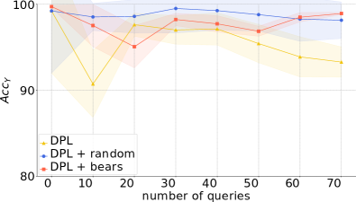
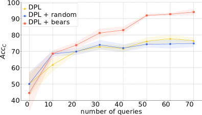
Figure 7: bears allows selecting informative concept annotations faster. (left) label accuracy. (right) concept accuracy.

C.4 Concept-wise Entropy scores for MNIST-Half

We report the entropy scores for each concept for all NeSy models we tested. bears performs as desired, whereas the runner-up, LA, struggles to put low-entropy on $0$, especially when paired with SL and LTN.

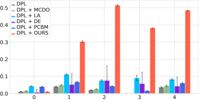
Figure 8: DPL + bears shows high entropy for concepts affected by RSs while it does not for others in out-of-distribution settings. (left In distribution. (right) Out-of-distribution

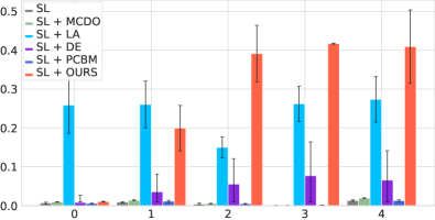
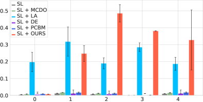
Figure 9: SL + bears shows high entropy for concepts affected by RSs while it does not for others. (left): in-distribution. (right): out-of-distribution.

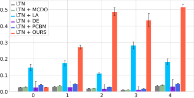
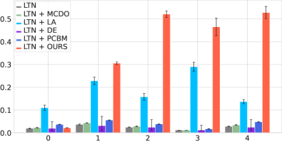
Figure 10: LTN + bears shows high entropy for concepts affected by RSs while it does not for others. (left): in-distribution. (right): out-of-distribution.

C.5 Confusion Matrices Kandinsky

We report the confusion matrices (CMs) for the active learning experiment on Kandinsky dataset. At the beginning, DPL picks a RS showing that only few concept vectors ${\bm{\mathrm{c}}}$ can be used to solve the classification task. At the last iteration, corresponding to collecting a total of $70$ objects with concept annotation, DPL and DPL + bears show very different CMs. Both show that colors have learned correctly, although the concept annotation collected with bears make DPL align more to the diagonal, corresponding to the intended solution.

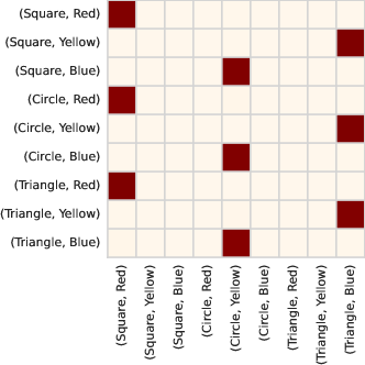
Figure 11: DPL at iteration $0$ in active learning settings on Kandinsky

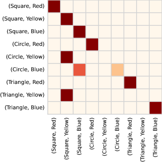
Figure 12: Iteration $70$ in active learning settings on Kandinsky. Right: DPL Left: DPL + bears

C.6 Confusion Matrices on BDD-OIA

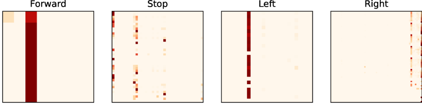
Figure 13: DPL confusion matrices per concept classes on BDD-OIA

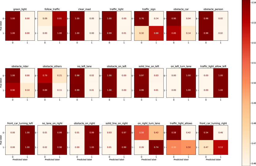
Figure 14: DPL multilabel confusion matrix on BDD-OIA

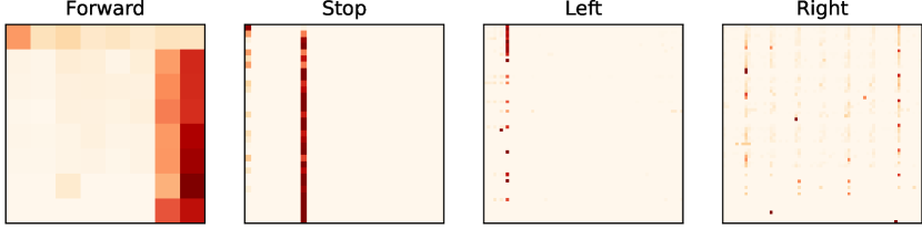
Figure 15: DPL + bears confusion matrices per concept classes on BDD-OIA

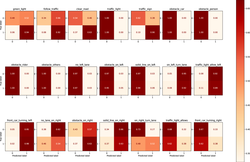
Figure 16: DPL + bears multilabel confusion matrix on BDD-OIA

C.7 Confusion Matrices on MNIST-Half

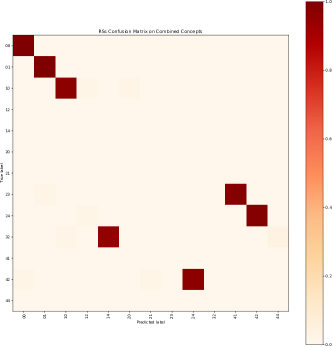
POLLO

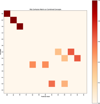
Figure 17: (left) DPL and (right) DPL + bears concepts confusion matrix on MNIST-Half

References

- Xu et al. [2020] Yiran Xu, Xiaoyin Yang, Lihang Gong, Hsuan-Chu Lin, Tz-Ying Wu, Yunsheng Li, and Nuno Vasconcelos. Explainable object-induced action decision for autonomous vehicles. In IEEE/CVF Conference on Computer Vision and Pattern Recognition (CVPR), June 2020.
- Sawada and Nakamura [2022] Yoshihide Sawada and Keigo Nakamura. Concept bottleneck model with additional unsupervised concepts. IEEE Access, 10:41758–41765, 2022.
- Marconato et al. [2023a] Emanuele Marconato, Stefano Teso, Antonio Vergari, and Andrea Passerini. Not all neuro-symbolic concepts are created equal: Analysis and mitigation of reasoning shortcuts. In NeurIPS, 2023a.
- Garcez et al. [2019] A Garcez, M Gori, LC Lamb, L Serafini, M Spranger, and SN Tran. Neural-symbolic computing: An effective methodology for principled integration of machine learning and reasoning. Journal of Applied Logics, 6(4):611–632, 2019.
- De Raedt et al. [2021] Luc De Raedt, Sebastijan Dumančić, Robin Manhaeve, and Giuseppe Marra. From statistical relational to neural-symbolic artificial intelligence. In Proceedings of the Twenty-Ninth International Conference on International Joint Conferences on Artificial Intelligence, pages 4943–4950, 2021.
- Garcez et al. [2022] Artur d’Avila Garcez, Sebastian Bader, Howard Bowman, Luis C Lamb, Leo de Penning, BV Illuminoo, Hoifung Poon, and COPPE Gerson Zaverucha. Neural-symbolic learning and reasoning: A survey and interpretation. Neuro-Symbolic Artificial Intelligence: The State of the Art, 342:1, 2022.
- Xu et al. [2018] Jingyi Xu, Zilu Zhang, Tal Friedman, Yitao Liang, and Guy Broeck. A semantic loss function for deep learning with symbolic knowledge. In ICML, 2018.
- Manhaeve et al. [2018] Robin Manhaeve, Sebastijan Dumancic, Angelika Kimmig, Thomas Demeester, and Luc De Raedt. DeepProbLog: Neural Probabilistic Logic Programming. NeurIPS, 2018.
- Giunchiglia and Lukasiewicz [2020] Eleonora Giunchiglia and Thomas Lukasiewicz. Coherent hierarchical multi-label classification networks. NeurIPS, 2020.
- Ahmed et al. [2022a] Kareem Ahmed, Stefano Teso, Kai-Wei Chang, Guy Van den Broeck, and Antonio Vergari. Semantic Probabilistic Layers for Neuro-Symbolic Learning. In NeurIPS, 2022a.
- Hoernle et al. [2022] Nick Hoernle, Rafael Michael Karampatsis, Vaishak Belle, and Kobi Gal. Multiplexnet: Towards fully satisfied logical constraints in neural networks. In AAAI, 2022.
- Di Liello et al. [2020] Luca Di Liello, Pierfrancesco Ardino, Jacopo Gobbi, Paolo Morettin, Stefano Teso, and Andrea Passerini. Efficient generation of structured objects with constrained adversarial networks. Advances in neural information processing systems, 33:14663–14674, 2020.
- Li et al. [2023] Zenan Li, Zehua Liu, Yuan Yao, Jingwei Xu, Taolue Chen, Xiaoxing Ma, L Jian, et al. Learning with logical constraints but without shortcut satisfaction. In ICLR, 2023.
- Wang et al. [2023] Kaifu Wang, Efi Tsamoura, and Dan Roth. On learning latent models with multi-instance weak supervision. In NeurIPS, 2023.
- Marconato et al. [2023b] Emanuele Marconato, Gianpaolo Bontempo, Elisa Ficarra, Simone Calderara, Andrea Passerini, and Stefano Teso. Neuro symbolic continual learning: Knowledge, reasoning shortcuts and concept rehearsal. In ICML, 2023b.
- Xie et al. [2022] Xuan Xie, Kristian Kersting, and Daniel Neider. Neuro-symbolic verification of deep neural networks. In IJCAI, 2022.
- Koh et al. [2020] Pang Wei Koh, Thao Nguyen, Yew Siang Tang, Stephen Mussmann, Emma Pierson, Been Kim, and Percy Liang. Concept bottleneck models. In International Conference on Machine Learning, pages 5338–5348. PMLR, 2020.
- Marconato et al. [2023c] Emanuele Marconato, Andrea Passerini, and Stefano Teso. Interpretability is in the mind of the beholder: A causal framework for human-interpretable representation learning. Entropy, 25(12):1574, 2023c.
- Poeta et al. [2023] Eleonora Poeta, Gabriele Ciravegna, Eliana Pastor, Tania Cerquitelli, and Elena Baralis. Concept-based explainable artificial intelligence: A survey. arXiv preprint arXiv:2312.12936, 2023.
- Teso et al. [2023] Stefano Teso, Öznur Alkan, Wolfang Stammer, and Elizabeth Daly. Leveraging explanations in interactive machine learning: An overview. Frontiers in Artificial Intelligence, 2023.
- Dash et al. [2022] Tirtharaj Dash, Sharad Chitlangia, Aditya Ahuja, and Ashwin Srinivasan. A review of some techniques for inclusion of domain-knowledge into deep neural networks. Scientific Reports, 12(1):1–15, 2022.
- Giunchiglia et al. [2022] Eleonora Giunchiglia, Mihaela Catalina Stoian, and Thomas Lukasiewicz. Deep learning with logical constraints. arXiv preprint arXiv:2205.00523, 2022.
- Ahmed et al. [2022b] Kareem Ahmed, Eric Wang, Kai-Wei Chang, and Guy Van den Broeck. Neuro-symbolic entropy regularization. In UAI, 2022b.
- van Krieken et al. [2022a] Emile van Krieken, Thiviyan Thanapalasingam, Jakub M Tomczak, Frank van Harmelen, and Annette ten Teije. A-nesi: A scalable approximate method for probabilistic neurosymbolic inference. arXiv preprint arXiv:2212.12393, 2022a.
- Koller and Friedman [2009] Daphne Koller and Nir Friedman. Probabilistic graphical models: principles and techniques. MIT press, 2009.
- Rudin [2019] Cynthia Rudin. Stop explaining black box machine learning models for high stakes decisions and use interpretable models instead. Nature Machine Intelligence, 1(5):206–215, 2019.
- Kambhampati et al. [2022] Subbarao Kambhampati, Sarath Sreedharan, Mudit Verma, Yantian Zha, and Lin Guan. Symbols as a Lingua Franca for Bridging Human-AI Chasm for Explainable and Advisable AI Systems. In Proceedings of Thirty-Sixth AAAI Conference on Artificial Intelligence (AAAI), 2022.
- Caruana [1997] Rich Caruana. Multitask learning. Machine learning, 28:41–75, 1997.
- Khemakhem et al. [2020] Ilyes Khemakhem, Diederik Kingma, Ricardo Monti, and Aapo Hyvarinen. Variational autoencoders and nonlinear ICA: A unifying framework. In International Conference on Artificial Intelligence and Statistics, pages 2207–2217. PMLR, 2020.
- Schölkopf et al. [2021] Bernhard Schölkopf, Francesco Locatello, Stefan Bauer, Nan Rosemary Ke, Nal Kalchbrenner, Anirudh Goyal, and Yoshua Bengio. Toward causal representation learning. Proceedings of the IEEE, 2021.
- Gresele et al. [2021] Luigi Gresele, Julius Von Kügelgen, Vincent Stimper, Bernhard Schölkopf, and Michel Besserve. Independent mechanism analysis, a new concept? Advances in neural information processing systems, 34:28233–28248, 2021.
- Lachapelle et al. [2024] Sébastien Lachapelle, Pau Rodríguez López, Yash Sharma, Katie Everett, Rémi Le Priol, Alexandre Lacoste, and Simon Lacoste-Julien. Nonparametric partial disentanglement via mechanism sparsity: Sparse actions, interventions and sparse temporal dependencies. arXiv preprint arXiv:2401.04890, 2024.
- Liang et al. [2023] Wendong Liang, Armin Kekić, Julius von Kügelgen, Simon Buchholz, Michel Besserve, Luigi Gresele, and Bernhard Schölkopf. Causal component analysis. arXiv preprint arXiv:2305.17225, 2023.
- Buchholz et al. [2023] Simon Buchholz, Goutham Rajendran, Elan Rosenfeld, Bryon Aragam, Bernhard Schölkopf, and Pradeep Ravikumar. Learning linear causal representations from interventions under general nonlinear mixing. arXiv preprint arXiv:2306.02235, 2023.
- Neal [2012] Radford M Neal. Bayesian learning for neural networks, volume 118. Springer Science & Business Media, 2012.
- Kendall and Gal [2017] Alex Kendall and Yarin Gal. What uncertainties do we need in bayesian deep learning for computer vision? Advances in neural information processing systems, 30, 2017.
- Wang and Yeung [2020] Hao Wang and Dit-Yan Yeung. A survey on bayesian deep learning. ACM computing surveys (csur), 53(5):1–37, 2020.
- Daxberger et al. [2021] Erik Daxberger, Agustinus Kristiadi, Alexander Immer, Runa Eschenhagen, Matthias Bauer, and Philipp Hennig. Laplace redux-effortless bayesian deep learning. Advances in Neural Information Processing Systems, 34:20089–20103, 2021.
- Osawa et al. [2019] Kazuki Osawa, Siddharth Swaroop, Mohammad Emtiyaz E Khan, Anirudh Jain, Runa Eschenhagen, Richard E Turner, and Rio Yokota. Practical deep learning with bayesian principles. Advances in neural information processing systems, 32, 2019.
- Lakshminarayanan et al. [2017] Balaji Lakshminarayanan, Alexander Pritzel, and Charles Blundell. Simple and scalable predictive uncertainty estimation using deep ensembles. In I. Guyon, U. Von Luxburg, S. Bengio, H. Wallach, R. Fergus, S. Vishwanathan, and R. Garnett, editors, Advances in Neural Information Processing Systems, volume 30. Curran Associates, Inc., 2017.
- Jospin et al. [2022] Laurent Valentin Jospin, Hamid Laga, Farid Boussaid, Wray Buntine, and Mohammed Bennamoun. Hands-on bayesian neural networks—a tutorial for deep learning users. IEEE Computational Intelligence Magazine, 17(2):29–48, 2022.
- D’Angelo and Fortuin [2021] Francesco D’Angelo and Vincent Fortuin. Repulsive deep ensembles are bayesian. Advances in Neural Information Processing Systems, 34:3451–3465, 2021.
- Wild et al. [2023] Veit David Wild, Sahra Ghalebikesabi, Dino Sejdinovic, and Jeremias Knoblauch. A rigorous link between deep ensembles and (variational) bayesian methods. In Thirty-seventh Conference on Neural Information Processing Systems, 2023. URL https://openreview.net/forum?id=eTHawKFT4h.
- Settles [2012] B. Settles. Active Learning. Synthesis lectures on artificial intelligence and machine learning. Morgan & Claypool, 2012. ISBN 9781608457250. URL https://books.google.it/books?id=z7toC3z_QjQC.
- Vergari et al. [2021] Antonio Vergari, YooJung Choi, Anji Liu, Stefano Teso, and Guy Van den Broeck. A compositional atlas of tractable circuit operations for probabilistic inference. Advances in Neural Information Processing Systems, 34, 2021.
- De Raedt and Kimmig [2015] Luc De Raedt and Angelika Kimmig. Probabilistic (logic) programming concepts. Machine Learning, 2015.
- Donadello et al. [2017] Ivan Donadello, Luciano Serafini, and Artur D’Avila Garcez. Logic tensor networks for semantic image interpretation. In IJCAI, 2017.
- Badreddine et al. [2022] Samy Badreddine, Artur d’Avila Garcez, Luciano Serafini, and Michael Spranger. Logic tensor networks. Artificial Intelligence, 303:103649, 2022.
- Gal and Ghahramani [2016] Yarin Gal and Zoubin Ghahramani. Dropout as a bayesian approximation: Representing model uncertainty in deep learning. In international conference on machine learning, pages 1050–1059. PMLR, 2016.
- Kim et al. [2023] Eunji Kim, Dahuin Jung, Sangha Park, Siwon Kim, and Sungroh Yoon. Probabilistic concept bottleneck models. arXiv preprint arXiv:2306.01574, 2023.
- LeCun [1998] Yann LeCun. The mnist database of handwritten digits. http://yann. lecun. com/exdb/mnist/, 1998.
- Müller and Holzinger [2021] Heimo Müller and Andreas Holzinger. Kandinsky patterns. Artificial Intelligence, 300:103546, November 2021. ISSN 0004-3702. doi:10.1016/j.artint.2021.103546. URL http://dx.doi.org/10.1016/j.artint.2021.103546.
- Misino et al. [2022] Eleonora Misino, Giuseppe Marra, and Emanuele Sansone. VAEL: Bridging Variational Autoencoders and Probabilistic Logic Programming. NeurIPS, 2022.
- Ahmed et al. [2023] Kareem Ahmed, Kai-Wei Chang, and Guy Van den Broeck. A pseudo-semantic loss for deep generative models with logical constraints. In Knowledge and Logical Reasoning in the Era of Data-driven Learning Workshop, July 2023.
- Lippi and Frasconi [2009] Marco Lippi and Paolo Frasconi. Prediction of protein -residue contacts by markov logic networks with grounding-specific weights. Bioinformatics, 2009.
- Yang et al. [2020] Zhun Yang, Adam Ishay, and Joohyung Lee. NeurASP: Embracing neural networks into answer set programming. In IJCAI, 2020.
- Huang et al. [2021] Jiani Huang, Ziyang Li, Binghong Chen, Karan Samel, Mayur Naik, Le Song, and Xujie Si. Scallop: From probabilistic deductive databases to scalable differentiable reasoning. NeurIPS, 2021.
- Marra and Kuželka [2021] Giuseppe Marra and Ondřej Kuželka. Neural markov logic networks. In Uncertainty in Artificial Intelligence, 2021.
- Skryagin et al. [2022] Arseny Skryagin, Wolfgang Stammer, Daniel Ochs, Devendra Singh Dhami, and Kristian Kersting. Neural-probabilistic answer set programming. In Proceedings of the International Conference on Principles of Knowledge Representation and Reasoning, volume 19, pages 463–473, 2022.
- Diligenti et al. [2017] Michelangelo Diligenti, Marco Gori, and Claudio Sacca. Semantic-based regularization for learning and inference. Artificial Intelligence, 2017.
- van Krieken et al. [2022b] Emile van Krieken, Erman Acar, and Frank van Harmelen. Analyzing differentiable fuzzy logic operators. Artificial Intelligence, 2022b.
- Rocktäschel and Riedel [2016] Tim Rocktäschel and Sebastian Riedel. Learning knowledge base inference with neural theorem provers. In Proceedings of the 5th workshop on automated knowledge base construction, pages 45–50, 2016.
- Pryor et al. [2022] Connor Pryor, Charles Dickens, Eriq Augustine, Alon Albalak, William Wang, and Lise Getoor. Neupsl: Neural probabilistic soft logic. arXiv preprint arXiv:2205.14268, 2022.
- Fischer et al. [2019] Marc Fischer, Mislav Balunovic, Dana Drachsler-Cohen, Timon Gehr, Ce Zhang, and Martin Vechev. Dl2: Training and querying neural networks with logic. In International Conference on Machine Learning, pages 1931–1941. PMLR, 2019.
- Giunchiglia et al. [2024] Eleonora Giunchiglia, Alex Tatomir, Mihaela Cătălina Stoian, and Thomas Lukasiewicz. Ccn+: A neuro-symbolic framework for deep learning with requirements. International Journal of Approximate Reasoning, page 109124, 2024.
- Manhaeve et al. [2021] Robin Manhaeve, Sebastijan Dumančić, Angelika Kimmig, Thomas Demeester, and Luc De Raedt. Neural probabilistic logic programming in deepproblog. Artificial Intelligence, 298:103504, 2021.
- Sansone and Manhaeve [2023] Emanuele Sansone and Robin Manhaeve. Learning symbolic representations through joint generative and discriminative training. In International Joint Conference on Artificial Intelligence 2023 Workshop on Knowledge-Based Compositional Generalization, 2023.
- Abdar et al. [2021] Moloud Abdar, Farhad Pourpanah, Sadiq Hussain, Dana Rezazadegan, Li Liu, Mohammad Ghavamzadeh, Paul Fieguth, Xiaochun Cao, Abbas Khosravi, U Rajendra Acharya, et al. A review of uncertainty quantification in deep learning: Techniques, applications and challenges. Information fusion, 76:243–297, 2021.
- Müller et al. [2019] Rafael Müller, Simon Kornblith, and Geoffrey E Hinton. When does label smoothing help? Advances in neural information processing systems, 32, 2019.
- Li et al. [2020] Qing Li, Siyuan Huang, Yining Hong, Yixin Chen, Ying Nian Wu, and Song-Chun Zhu. Closed loop neural-symbolic learning via integrating neural perception, grammar parsing, and symbolic reasoning. In International Conference on Machine Learning, pages 5884–5894. PMLR, 2020.
- Wei et al. [2022] Hongxin Wei, Renchunzi Xie, Hao Cheng, Lei Feng, Bo An, and Yixuan Li. Mitigating neural network overconfidence with logit normalization. In International Conference on Machine Learning, pages 23631–23644. PMLR, 2022.
- Mukhoti et al. [2020] Jishnu Mukhoti, Viveka Kulharia, Amartya Sanyal, Stuart Golodetz, Philip Torr, and Puneet Dokania. Calibrating deep neural networks using focal loss. Advances in Neural Information Processing Systems, 33:15288–15299, 2020.
- Carratino et al. [2022] Luigi Carratino, Moustapha Cissé, Rodolphe Jenatton, and Jean-Philippe Vert. On mixup regularization. The Journal of Machine Learning Research, 23(1):14632–14662, 2022.
- Marconato et al. [2022] Emanuele Marconato, Andrea Passerini, and Stefano Teso. Glancenets: Interpretabile, leak-proof concept-based models. NeurIPS, 2022.
- Collins et al. [2023] Katherine Maeve Collins, Matthew Barker, Mateo Espinosa Zarlenga, Naveen Raman, Umang Bhatt, Mateja Jamnik, Ilia Sucholutsky, Adrian Weller, and Krishnamurthy Dvijotham. Human uncertainty in concept-based ai systems. In Proceedings of the 2023 AAAI/ACM Conference on AI, Ethics, and Society, pages 869–889, 2023.
- Kingma and Ba [2015] Diederik P. Kingma and Jimmy Ba. Adam: A method for stochastic optimization. In Yoshua Bengio and Yann LeCun, editors, 3rd International Conference on Learning Representations, ICLR 2015, San Diego, CA, USA, May 7-9, 2015, Conference Track Proceedings, 2015. URL http://arxiv.org/abs/1412.6980.
- Ren et al. [2015] Shaoqing Ren, Kaiming He, Ross Girshick, and Jian Sun. Faster r-cnn: Towards real-time object detection with region proposal networks. In C. Cortes, N. Lawrence, D. Lee, M. Sugiyama, and R. Garnett, editors, Advances in Neural Information Processing Systems, volume 28. Curran Associates, Inc., 2015. URL https://proceedings.neurips.cc/paper_files/paper/2015/file/14bfa6bb14875e45bba028a21ed38046-Paper.pdf.