Modeling the mechanisms of antibody mixtures in viral infections: the cases of sequential homologous and heterologous dengue infections

Abstract

Antibodies play an essential role in the immune response to viral infections, vaccination, or antibody therapy. Nevertheless, they can be either protective or harmful during the immune response. In addition, competition or cooperation between antibodies, when mixed, can enhance or reduce this protective or harmful effect. Using the laws of chemical reactions to model the binding of antibodies to antigens and their actions to neutralize or enhance infection, we propose a new approach to modeling the activity of the antigen-antibody complex. The resulting expression covers not only purely competitive or purely independent binding between antibodies but also synergistic binding which, depending on the type of antibody, can promote either neutralization or enhancement of the viral activity. We then integrate this expression of viral activity in a within-host model, an ordinary differential system, involving both healthy and infected target cells, virus replication, and the production of two antibodies during sequential infections. We investigate the existence of steady-states (disease-free and endemic) and their local and global asymptotic stability. We complete our study with numerical simulations to illustrate different scenarios. In particular, the scenario where both antibodies are neutralizing (homologous sequential DENV infection) and the scenario where one antibody is neutralizing and the other enhancing (heterologous sequential DENV infection). Our model indicates that efficient viral neutralization is associated with purely independent antibody binding, whereas strong enhancement of viral activity is expected in the case of purely competitive antibody binding. The model developed here has several potential applications for a variety of viral infections involving different antibody molecules. It could also be useful for studying the efficacy of vaccines and antibody-based therapies, for example for HIV.

1 Introduction

Active immunity is triggered by the entrance of a pathogen or by vaccination and involves the production of antibodies by the immune system. On the other hand, passive immunity involves the vertical transmission of antibodies from mother to offspring or the horizontal transmission of antibodies from humans or animals to susceptible individuals through antibody donation (antibody therapy). The interaction between the antibody and the antigen occurs through a specific chemical reaction, to form an antigen-antibody complex. This immune complex can either neutralize or enhance the activity of the pathogen. The strength of the antigen-antibody complex depends firstly on the affinity of the antibody for the antigen, secondly on the number of antigen-antibody binding sites, and thirdly on the structural arrangement of the interacting parts, [11, 33].

In the case of secondary infection by a homologous or heterologous virus, pre-existing antibodies and newly produced antibodies may coexist, [16]. In most cases, an active infection leads to the production of neutralizing antibodies. However, cross-reaction of pre-existing antibodies may or may not help neutralize this active infection; in fact, it has been observed that cross-reacting antibodies can enhance the infection, [8, 12, 29, 37, 40]. In the case of influenza, dengue, or Covid-19, for example, it has been observed that two successive homologous infections can increase the neutralizing effect of antibodies, [11, 28]. On the other hand, secondary infection with a heterologous dengue serotype may increase the risk of developing a severe form of the disease, due to Antibody-Dependent Enhancement (ADE) phenomenon, [8, 12, 13, 15, 23, 29, 37, 40]. Furthermore, in the presence of a mixture of two antibodies and a pathogen, two other factors come into play: (i) the competition between antibodies to bind to the antigen, and (ii) the synergistic interactions between antibodies, [11, 32]. This leads to three distinct types of antigen-antibody binding: (a) purely independent binding, where the binding of one antibody does not affect the binding of other antibodies to the same receptor; (b) purely competitive binding, where the two antibodies cannot bind simultaneously to the same receptor; and (c) an intermediate situation, where the two antibodies can bind simultaneously to many sites of the same receptor, with synergistic interactions, i.e., the binding of one has an effect on the binding of the other, either by making it weaker or stronger, [11, 32].

Several mathematical within-host infectious disease models have been developed to study the dynamics of viral infections and their interaction with the immune system, [2, 3, 6, 7, 14, 22, 24, 26, 41]. They involve, according to each paper, healthy and infected target cells, intracellular pathogen replication, T-cells, B-cells, cytokine production, and antibodies. Most of them resemble epidemiological models and use the mass action law or a saturation function to model the force of infection. In general, only one of the immune responses - humoral or cellular - is modeled, and very few models address interaction among components of the immune response. As an example, [2, 7, 22] took into account only one component of the immune system: T-cells, the only ones capable of killing infected cells. In particular, [2] used the Beddington-DeAngelis incidence rate to model interaction between susceptible cells and free viruses. They argued that they could thus reduce the time needed for the immune response to clean the dengue virus, compared with using the mass action law of the paper [22]. In both articles, depending on parameter values, more than one endemic steady-state was found, and thresholds for the stability of each of them have been attained. In [7], the authors used data coming from hospitalized primary and secondary dengue patients - virus viremia - to estimate model parameters that confirmed the role of the immune response in shaping variation between individuals consistent with the hypothesis of ADE. In [14], the authors considered heterologous antibodies that interact through a Heaviside step function that triggers neutralization or enhancement of the infection depending on the amount of the antibody from the first infection. The model also considered a delay in the immune response which switches the stability of the system through a Hopf bifurcation. The authors argued that they could qualitatively replicate the humoral immune responses observed in primary and secondary infections. The authors of [3] have shown that the risk of developing a severe form of dengue may be related to increased cytokine production due to the interaction of the immune system (T-cells) with the dengue virus. The model was parameterized to reproduce qualitatively the data set described in [7]. The virological indicators used were the level of peak viremia, the time to peak viremia, and the viral clearance rate. Although the model did not consider the humoral immune response explicitly, the authors argue that the reparametrization of the infectivity rate can be biologically interpreted in the context of the ADE phenomenon.

Other original approaches have been developed in [1, 4, 6]. All, explicitly considered interactions among susceptible and infected target cells, dengue virus, and dengue antibodies through bilinear and trilinear terms. In [6], two thresholds were obtained: the mean number of virions produced by one invading virus in the very early stage of secondary infection, and the rate at which one infected macrophage dies. The existence and stability of the endemic equilibrium depend on both parameters, and one of them acts as a weakening factor for ADE. In [1], the authors explored the occurrence of Dengue Hemorrhagic Fever (DHF) in infants born from dengue-immune mothers, during their first dengue infection. The neutralization and enhancement activities of maternal antibodies against the virus are represented by a function derived from experimental data. They were able to fit the model to data on the amount of maternal antibodies and the age of the infant at which DHF was reported. The authors were thus able to reproduce the time delay observed between the end of the protective level of maternal antibodies and the onset of hemorrhagic fever, in agreement with data from the literature. The article [4] focused on the ADE hypothesis and developed a mathematical model of secondary dengue infection by a different viral serotype. It considered indirect competition between neutralizing and enhancing antibodies. Here, the enhancement and neutralization functions are derived from basic concepts of chemical reactions and used to model virus-antibody complexes binding formed by distinct populations of antibodies, classified as cross-reactive or type-specific ones. The authors of this article concluded that virus-antibody immune complexes may promote viral clearance or enhancement of infection depending on the amount of cross-reacting antibodies and the rapid activation of the neutralizing antibodies.

The authors of [26, 41] considered the modeling of within-host dynamics of HIV infection and therapy. Both are review articles and can give a broad understanding of how the immune system interacts with viruses and the state of the art of HIV modeling which includes virus evolution. The authors claimed that HIV viruses have several different epitopes that can be recognized by immune responses. Furthermore, different populations of HIV viruses and antibodies when mixed, may have cross-reactive responses. In [24], the proposed model includes both innate and adaptive immune responses, during an influenza virus infection. Different from the other models, a class of uninfected cells that are refractory to infections was included. Modeling predictions were compared with both interferon and viral kinetic data. The first post-peak viral decline is explained by the lysis of infected cells during the innate immune response, the subsequent viral plateau/second peak is generated by the loss of the IFN-induced antiviral effect and the increased availability of target cells.

None of the cited works either considered the direct competition of the antibodies for the virus epitope or the synergistic interaction between antibodies. Therefore, the work presented here aims to introduce a new formalism, inspired by [11, 32], to efficiently describe the formation of antigen-antibody complexes, and to use it in a mathematical model to describe the interaction between a virus, target cells and two antibodies competing to bind to virus receptors, taking into account their synergistic interaction, and the effectiveness of the complex formed in neutralizing or enhancing the virus. To achieve this, we first consider a monoclonal antibody and define the viral activity function of the antigen-antibody complex. We then consider a mixture of two antibodies and generalize the viral activity function obtained previously, which now depends on the concentration of the two antibodies and the interaction between them. Finally, we use this viral activity function in a within-host infectious disease model. We then give some basic properties of the within-host model obtained, in particular the existence of steady-states (disease-free and endemic). We then investigate the local and global asymptotic stability of these steady-states. We complete our study with numerical simulations to highlight various scenarios. Although we have parameterized the model to study homologous and heterologous secondary infection with the dengue virus, it can be easily adapted to other viruses. It can also be extended to vaccination or antibody therapy, [19, 34].

2 Modeling the antigen-antibody complex

2.1 Monoclonal antibody binding to a receptor

Consider a monoclonal antibody $A$ that binds to an antigen $R$ (viral receptor) through a paratope-epitope bond and, depending on its affinity, inhibits or enhances viral activity. An antibody can recognize a number $n$ of epitopes of the same antigen, [23]. Antigen-antibody binding occurs through a chemical reaction, [11], in which $n$ paratopes $N$ of $A$ bind to $n$ epitopes of $R$. According to the standard law of mass action, the process leading to this bond is given by the following sequential chemical reaction:

$$R+nN\xrightleftharpoons[k^{-}]{nk^{+}}{R_{1N}}+(n-1)N\xrightleftharpoons[2k^{-}]{(n-1)k^{+}}\dots\xrightleftharpoons[ik^{-}]{(n-i+1)k^{+}}R_{iN}+(n-i)N\xrightleftharpoons[(i+1)k^{-}]{(n-i)k^{+}}\dots\xrightleftharpoons[nk^{-}]{k^{+}}R_{nN},$$ (1)

where $R_{iN}$ stands for the complex formed by $i$ epitopes of $R$ bound by $i$ paratopes $N$ of $A$, $R=R_{0N}$ means free antigen, $k^{+}$ and $k^{-}$ denotes the forward and backward reaction rates, [25]. When the chemical reaction reaches equilibrium, we obtain the following equation

$$(n-i)k^{+}[R_{iN}][N]^{n-i}=(i+1)k^{-}[R_{(i+1)N}][N]^{n-i-1},$$

valid for $i\in\{0,1,\dots,n-1\}$, where $[\cdot]$ is the concentration of the chemical species. After some algebraic manipulation, we get

$$[R_{iN}]=\dfrac{n-i+1}{i}\dfrac{[N]}{K}[R_{(i-1)N}],\quad\text{for }i\in\{1,\dots,n\},$$

where $K=k^{-}/k^{+}$ is the dissociation constant of the reaction. Solving this recurrence equation yields to

$$[R_{iN}]=C^{i}_{n}\left([N]/K\right)^{i}[R],$$

with $C^{i}_{n}=\frac{n!}{i!(n-i)!}$, the binomial coefficient. Given the total antigen concentration,

$$[R_{\text{total}}]=\sum_{i=0}^{n}[R_{iN}]=\left(1+\dfrac{[N]}{K}\right)^{n}[R]$$

and that the antibody concentration $A$ is proportional to the concentration of paratope $N$, $A=\theta[N]$, the fraction of occupied epitopes of the antigen is

$$\frac{[R_{iN}]}{[R_{\text{total}}]}=\dfrac{C^{i}_{n}(A/K_{D})^{i}}{(1+A/K_{D})^{n}},$$ (2)

with $K_{D}=\theta K$, where $\theta$ is a constant. The antigen-antibody complex modifies viral activity. Let’s define the relative activity of a virus belonging to this complex as $\xi_{i}\geq 0$, where $i$ represents the number of occupied epitopes of the antigen. The value $0<\xi_{i}<1$ means that the complex antigen-antibody partially inhibits virus activity, while $\xi_{i}>1$ means that it increases virus activity. The case $\xi_{i}=1$ means that the relative activity remains unchanged. In particular, $\xi_{0}=1$, because no antigen-antibody complex is formed. Therefore, the activity of the virus is obtained by adding the products of the fractions (2) by their associated relative activities $\xi_{i}$,

$$\text{Activity}:=G(A)=\sum_{i=0}^{n}\xi_{i}\times\dfrac{C^{i}_{n}(A/K_{D})^{i}}{(1+A/K_{D})^{n}}=\dfrac{1+\sum_{i=1}^{n}\xi_{i}C^{i}_{n}(A/K_{D})^{i}}{1+\sum_{i=1}^{n}C^{i}_{n}(A/K_{D})^{i}}.$$ (3)

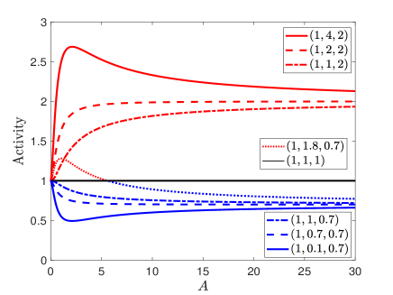
Figure 1: Viral activity as a function of monoclonal antibody $A$, with $K_{D}=0.7$ and $n=3$ and for different values of relative viral activities $(\xi_{1},\xi_{2},\xi_{3})$. Red curves highlight the antigen-antibody complex leading to enhancement, while blue curves are those leading to neutralization. The black curve means that virus activity is neither neutralized nor enhanced. Depending on the amount of antibody, virus activity can change from enhancement to neutralization (red-blue curve).

The binding affinity between the antigen’s epitope and the antibody’s paratope at a single binding site can be interpreted in different ways. For example, the higher the affinity, the lower the values of $K_{D}$ and $\xi_{i}$. This explains the property of neutralizing antibodies, which have a high affinity for the virus and, after binding to the receptor, neutralize it, $G(A)<1$ (blue lines in Figure 1). Non-neutralizing cross-reactive antibodies, on the other hand, only partially recognize the receptor (low affinity), [23]. The constant $K_{D}$ is therefore high, and $\xi_{i}$ are close to $1$. In particular, if all relative activities $\xi_{i}$ are equal to $1$, the virus activity remains unaffected, $G(A)=1$ (black line in Figure 1). For some viral infections, such as secondary dengue infection, non-neutralizing cross-reactive antibodies may enhance the infection. This means an increase in viral activity, $G(A)>1$ (red lines in Figure 1). As the interaction antigen-antibody is a multi-hit phenomenon, [27], enhancement can occur for an intermediate amount of antibody, while neutralization occurs in the presence of a sufficiently large amount of antibody, [10, 17]. This suggests that if the number of occupied epitopes is high enough, epitope-paratope binding will neutralize antigen activity; and if the number of occupied epitopes is intermediate, this binding will tend to enhance antigen activity (the curve in Figure 1 that starts red, then becomes blue).

2.2 Binding of a mixture of two antibodies to a receptor

In [11], the authors have developed a statistical mechanical model that predicts the collective efficacy of a mixture of antibodies whose constituents are assumed to bind to a single site on a receptor. We generalize their method to the case where the mixture can bind to multiple sites on a receptor, [23]. Let’s consider now a mixture of two different antibodies $A_{1}$, $A_{2}$ that interact with a virus receptor $R$. This mixture can result in an antigen-antibody complex with purely independent bindings, purely competitive bindings, or synergistic bindings. This binding classification is based on the interactions (competition/cooperation) between the two antibodies. In this case, the activity of the virus is defined by the function $G(A_{1},A_{2})$, given by,

$$G(A_{1},A_{2})=\dfrac{1+\displaystyle\sum_{i=1}^{n_{1}}\xi_{1i}C^{i}_{n_{1}}\left(\frac{A_{1}}{K_{D_{1}}}\right)^{i}+\displaystyle\sum_{j=1}^{n_{2}}\xi_{2j}C^{j}_{n_{2}}\left(\frac{A_{2}}{K_{D_{2}}}\right)^{j}+\displaystyle\sum_{i=1}^{n_{1}}\displaystyle\sum_{j=1}^{n_{2}}f_{ij}\tilde{\xi}_{1i}\tilde{\xi}_{2j}C^{i}_{n_{1}}C^{j}_{n_{2}}\left(\frac{A_{1}}{\tilde{K}_{D_{1}}}\right)^{i}\left(\frac{A_{2}}{\tilde{K}_{D_{2}}}\right)^{j}}{1+\displaystyle\sum_{i=1}^{n_{1}}C^{i}_{n_{1}}\left(\dfrac{A_{1}}{K_{D_{1}}}\right)^{i}+\displaystyle\sum_{j=1}^{n_{2}}C^{j}_{n_{2}}\left(\frac{A_{2}}{K_{D_{2}}}\right)^{j}+\displaystyle\sum_{i=1}^{n_{1}}\displaystyle\sum_{j=1}^{n_{2}}f_{ij}C^{i}_{n_{1}}C^{j}_{n_{2}}\left(\frac{A_{1}}{\tilde{K}_{D_{1}}}\right)^{i}\left(\frac{A_{2}}{\tilde{K}_{D_{2}}}\right)^{j}}.$$ (4)

As in (2), $n_{1}$ (resp. $n_{2}$) is the number of epitopes of the antigen that can be recognized by the antibody $A_{1}$ (resp. $A_{2}$), $\xi_{1i}$ (resp. $\xi_{2j}$) is the relative activity of the virus when bound to $i$ paratopes of $A_{1}$ (resp. $j$ paratopes of $A_{2}$), and $K_{D_{1}}$ (resp. $K_{D_{2}}$) is the dissociation constant associated to the antibody $A_{1}$ (resp. $A_{2}$). The new parameters $\tilde{\xi}_{1i}$, $\tilde{\xi}_{2j}$ are the relative virus activities modified by a synergistic binding (the relative virus activity may decrease in the presence of the other antibody because of competition, $\tilde{\xi}_{kl}<\xi_{kl}$, or it can increase because of cooperation, $\tilde{\xi}_{kl}>\xi_{kl}$). Similarly, a synergistic interaction between two antibodies can modify their binding to the receptor and thus their dissociation constants $K_{D_{k}}$, $k=1,2$. We then introduce modified dissociation constants $\tilde{K}_{D_{k}}$, with $\tilde{K}_{D_{k}}<K_{D_{k}}$ when antigen-antibody binding becomes stronger and $\tilde{K}_{D_{k}}>K_{D_{k}}$ when antigen-antibody binding becomes weaker. The coefficient $0\leq f_{ij}\leq 1$ corresponds to the fraction of simultaneous binding of both antibodies. Thus, three scenarios are possible: (i) purely competitive binding, with $f_{ij}=0$; (ii) synergistic binding, where $0<f_{ij}\leq 1$; and (iii) purely independent binding, where $f_{ij}=1$, $\tilde{\xi}_{ki}=\xi_{ki}$ and $\tilde{K}_{D_{k}}=K_{D_{k}}$, for $k=1,2$, $i=1,\dots,n_{1}$ and $j=1,\dots,n_{2}$. In the case of [11], $n_{1}=n_{2}=1$. The purely competitive binding and the purely independent binding lead respectively to the following expressions of the virus activity

$$G(A_{1},A_{2})=\dfrac{1+\displaystyle\sum_{i=1}^{n_{1}}\xi_{1i}C^{i}_{n_{1}}\left(\dfrac{A_{1}}{K_{D_{1}}}\right)^{i}+\displaystyle\sum_{j=1}^{n_{2}}\xi_{2j}C^{j}_{n_{2}}\left(\dfrac{A_{2}}{K_{D_{2}}}\right)^{j}}{1+\displaystyle\sum_{i=1}^{n_{1}}C^{i}_{n_{1}}\left(\dfrac{A_{1}}{K_{D_{1}}}\right)^{i}+\displaystyle\sum_{j=1}^{n_{2}}C^{j}_{n_{2}}\left(\dfrac{A_{2}}{K_{D_{2}}}\right)^{j}},$$ (5)

and

$$G(A_{1},A_{2})=\left(\dfrac{1+\displaystyle\sum_{i=1}^{n_{1}}\xi_{1i}C^{i}_{n_{1}}\left(\dfrac{A_{1}}{K_{D_{1}}}\right)^{i}}{\left(1+\dfrac{A_{1}}{K_{D_{1}}}\right)^{n_{1}}}\right)\times\left(\dfrac{1+\displaystyle\sum_{j=1}^{n_{2}}\xi_{2i}C^{i}_{n_{2}}\left(\dfrac{A_{2}}{K_{D_{2}}}\right)^{j}}{\left(1+\dfrac{A_{2}}{K_{D_{2}}}\right)^{n_{2}}}\right).$$ (6)

To study the synergistic binding effect on viral activity, we introduce the following notations $\tilde{\nu}_{ij}=\tilde{\xi}_{1i}\tilde{\xi}_{2j}/(\xi_{1i}\xi_{2j})$ and $\tilde{\kappa}_{ij}=K_{D_{1}}^{i}K_{D_{2}}^{j}/(\tilde{K}_{D_{1}}^{i}\tilde{K}_{D_{2}}^{j})$, and explore the values of these relative quantities. The expression (4) becomes

$$G(A_{1},A_{2})=\dfrac{1+\displaystyle\sum_{i=1}^{n_{1}}\xi_{1i}C^{i}_{n_{1}}\left(\frac{A_{1}}{K_{D_{1}}}\right)^{i}+\displaystyle\sum_{j=1}^{n_{2}}\xi_{2j}C^{j}_{n_{2}}\left(\frac{A_{2}}{K_{D_{2}}}\right)^{j}+\displaystyle\sum_{i=1}^{n_{1}}\displaystyle\sum_{j=1}^{n_{2}}\tilde{\nu}_{ij}\tilde{\kappa}_{ij}f_{ij}\xi_{1i}\xi_{2j}C^{i}_{n_{1}}C^{j}_{n_{2}}\left(\frac{A_{1}}{K_{D_{1}}}\right)^{i}\left(\frac{A_{2}}{K_{D_{2}}}\right)^{j}}{1+\displaystyle\sum_{i=1}^{n_{1}}C^{i}_{n_{1}}\left(\dfrac{A_{1}}{K_{D_{1}}}\right)^{i}+\displaystyle\sum_{j=1}^{n_{2}}C^{j}_{n_{2}}\left(\frac{A_{2}}{K_{D_{2}}}\right)^{j}+\displaystyle\sum_{i=1}^{n_{1}}\displaystyle\sum_{j=1}^{n_{2}}\tilde{\kappa}_{ij}f_{ij}C^{i}_{n_{1}}C^{j}_{n_{2}}\left(\frac{A_{1}}{K_{D_{1}}}\right)^{i}\left(\frac{A_{2}}{K_{D_{2}}}\right)^{j}}.$$ (7)

The new parameters $\tilde{\nu}_{ij}$ and $\tilde{\kappa}_{ij}$ can be interpreted as follows. If $\tilde{\nu}_{ij}<1$, the relative viral activity due to synergistic binding decreases. On the other hand, if $\tilde{\nu}_{ij}>1$, relative viral activity increases. Furthermore, if $\tilde{\kappa}_{ij}<1$, the binding between the antibodies and the virus is enhanced by synergistic binding, and if $\tilde{\kappa}_{ij}<1$ this binding becomes weaker. In theory, many combinations are possible, but we will explore the most relevant ones: when both antibodies neutralize the virus activity, and when one antibody neutralizes and the other enhances the virus activity.

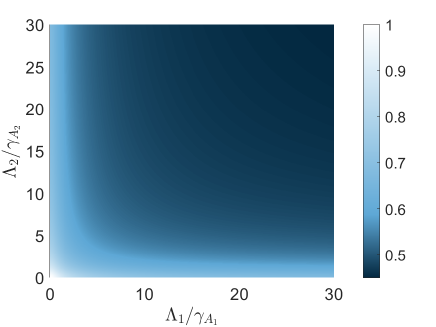
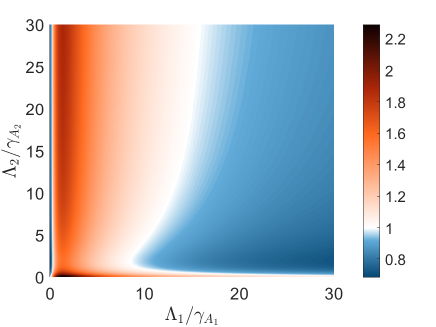
Figure 2: Viral activity $G(\Lambda_{1}/\gamma_{A_{1}},\Lambda_{2}/\gamma_{A_{2}})$, in the case of Neutralizing/Neutralizing (left panel) and Enhancing/Neutralizing (right panel). The palette of colors, from blue (neutralization) to red (enhancement), reflects the variation in viral activity on antigen-antibody complexes.

In Figure 2, we have chosen to represent the viral activity as a function of the components $\Lambda_{1}/\gamma_{A_{1}}$ and $\Lambda_{2}/\gamma_{A_{2}}$ because they represent the disease-free equilibrium when we choose $p_{i}(Y)=\Lambda_{i}+\alpha_{i}Y$, enabling us to measure the state of viral activity at this point. In the left panel of Figure 2 it is shown the variation in viral activity when both antibodies neutralize the virus. Whatever the direction, horizontal or vertical from the border, we always move towards lower viral activity, which means more neutralization. This is coherent with the assertion of [11, 28] that two antibodies are more effective than one in neutralizing a virus. In the right panel of Figure 2, it is shown the variation in viral activity in the case of enhancing antibody $A_{1}$ and neutralizing antibody $A_{2}$. For each fixed amount of neutralizing antibody, $\Lambda_{2}/\gamma_{A_{2}}$, viral activity first increases very rapidly as the amount of enhancing antibody $\Lambda_{1}/\gamma_{A_{1}}$ increases, reaching a peak in the red zone, then slowly decreases (moving from red to blue) until reaches a threshold in the blue (same behavior of the red/blue line of Figure 1). On the other hand, if we fix the amount of enhancing antibody, $\Lambda_{1}/\gamma_{A_{1}}$, and increase the amount of the neutralizing one, $\Lambda_{2}/\gamma_{A_{2}}$, we have the same shape as the solid blue curve of Figure 1 and we obtain different scenarios: (i) If $\Lambda_{1}/\gamma_{A_{1}}$ is fixed at a low or high level, viral activity will decrease rapidly at first, then reach a certain value (remain in the blue zone once entered, meaning that viral activity is neutralized); (ii) If $\Lambda_{1}/\gamma_{A_{1}}$ is fixed at an intermediate level, viral activity will start at a high level and change very quickly from red to blue or from dark red to light red, then return to an intermediate value and remain at this level. The main information to be deduced from the right panel of Figure 2 is that infection is more severe when the amount of enhancing antibodies is in the intermediate range. This is compatible with the assertion of [4, 10, 17] that the risk of severe dengue in a secondary infection is higher when there is an intermediate amount of pre-existing antibodies from the first infection. The common values of the parameters in Figure 2 are $K_{D_{1}}=\tilde{K}_{D_{1}}=K_{D_{2}}=\tilde{K}_{D_{2}}=0.7$ mol ml^-1, $\beta=8\times 10^{-9}$ ml RNA copies^-1, and $f_{ij}=1$. In the left panel of Figure 2, we take $(\xi_{11},\xi_{12},\xi_{13})=(\tilde{\xi}_{11},\tilde{\xi}_{12},\tilde{\xi}_{13})=(1,0.95,0.65)$ and $(\xi_{21},\xi_{22},\xi_{23})=(\tilde{\xi}_{21},\tilde{\xi}_{22},\tilde{\xi}_{23})=(1,0.95,0.65)$ ; and in the right panel of Figure 2, we take $(\xi_{11},\xi_{12},\xi_{13})=(\tilde{\xi}_{11},\tilde{\xi}_{12},\tilde{\xi}_{13})=(1,4,0.85)$, and $(\xi_{21},\xi_{22},\xi_{23})=(\tilde{\xi}_{21},\tilde{\xi}_{22},\tilde{\xi}_{23})=(1,0.4,0.85)$.

3 Within-host (re)infection dynamics in the presence of a mixture of two antibodies

Let’s consider a viral (re)infection at the cellular and immune level with a mixture of two antibodies. We note by $A_{1}$ the concentration of pre-existing antibody due to the first infection and by $A_{2}$ the concentration of the new antibody generated by the secondary infection with a homologous or heterologous virus. The quantities $X$ and $Y$ are the susceptible and infected target cells respectively, and $V$ is the free virus. Target cells may be epithelial cells in the case of influenza, [20] or macrophages and dendritic cells in the case of dengue, [21]. The model is described by the ordinary differential system given by

$$\left\{\begin{aligned} \dfrac{dA_{1}}{dt}&=p_{1}(Y)-\gamma_{A_{1}}A_{1},\\ \dfrac{dA_{2}}{dt}&=p_{2}(Y)-\gamma_{A_{2}}A_{2},\\ \dfrac{dX}{dt}&=\Omega-\gamma_{X}X-\beta G(A_{1},A_{2})VX,\\ \frac{dY}{dt}&=\beta G(A_{1},A_{2})VX-\gamma_{Y}Y,\\ \dfrac{dV}{dt}&=\Phi Y-(\delta+\gamma_{V})V.\end{aligned}\right.$$ (8)

The antibodies $A_{i}$ can be produced by memory B-cells or by plasmablasts upon stimulation by the virus or by infected cells, [9]. In the case of a secondary viral infection, the first antibody $A_{1}$ is generated mainly by memory B-cells, while the second antibody $A_{2}$ is generated mainly by plasmablasts. It is reasonable to assume that the production of both antibodies depends on the concentration of infected cells. The production of antibody $A_{i}$ is then considered with a rate equal to $p_{i}(Y)$, $p_{i}$ being a nonnegative, continuous, and nondecreasing function on $[0,+\infty)$. For all numerical simulations, we use the function $p_{i}(Y)=\Lambda_{i}+\alpha_{i}Y$. The natural mortality rates are denoted by $\gamma_{A_{i}}$, $\gamma_{X}$, $\gamma_{Y}$ and $\gamma_{V}$. The parameter $\Omega$ is the rate of production of susceptible target cells, which are generally produced in the bone marrow, [38]. $\Phi$ is the rate of virus production by infected cells, [30, 31]. The parameter $\delta$ represents the rate of free virus loss by other means than natural mortality, such as neutralization or entry into target cells. When the two antibodies $A_{1}$ and $A_{2}$ interact with the virus, its activity may decrease or increase depending on the nature of these antibodies. This activity has been defined in Subsection 2.2 by the function $G(A_{1},A_{2})$ given by (4). Then, the force of infection is $\beta G(A_{1},A_{2})V$, with $\beta>0$. This system can model a homologous or heterologous secondary viral infection, such as dengue fever or influenza. It can also be adapted to antiretroviral therapy in the case of HIV, provided we change the functions $p_{i}$ and adapt the parameter values.

Throughout this paper, we will need to make certain assumptions.

1. $\gamma:=\gamma_{X}=\gamma_{Y}$.

2. $\gamma_{A}:=\gamma_{A_{1}}=\gamma_{A_{2}}$.

3. $G\left(A_{1},A_{2}\right)\leq G\left(\frac{p_{1}(0)}{\gamma_{A_{1}}},\frac{p_{2}(0)}{\gamma_{A_{2}}}\right),\quad\text{for all }\left(A_{1},A_{2}\right)\in\mathbb{D},$ with

   $$\mathbb{D}:=\left\{(A_{1},A_{2})\in\mathbb{R}^{2}_{+}:A_{1}\geq\dfrac{p_{1}(0)}{\gamma_{A_{1}}},\;A_{2}\geq\dfrac{p_{2}(0)}{\gamma_{A_{2}}}\right\}.$$

4. $p_{i}(Y)-p_{i}(0)\leq p_{i}^{\prime}(0)Y$, for $i=1,2$, and all $Y\geq 0.$

5. $p_{1}^{\prime}(0)>0$ or $p_{2}^{\prime}(0)>0.$

The assumptions (H1) and (H2), mean that the disease does not affect cell mortality and that both antibodies have the same mortality rate. They are used, for the sake of simplicity, in the proof of the global asymptotic stability of $P_{0}$ and/or in the proof of the local asymptotic stability of $P^{\star}$, the disease-free equilibrium and the endemic one, respectively. Under (H3), quantities of antibodies $A_{1}$ and $A_{2}$ higher than those of the disease-free equilibrium reduce viral activity. This gives an advantage to neutralization. Hypothesis (H4) means that the dynamic of antibody production follows, at best, a linear growth. If (H5) is satisfied, then $p_{1}$ or $p_{2}$ is strictly increasing in a neighborhood of $0$, which implies a production strictly positive of $A_{1}$ or $A_{2}$ around $0$. The hypotheses (H3), (H4) and (H5) are assumed satisfied in Theorem 2 and Theorem 4. We assume throughout this article that $p_{i}$ is a $\mathcal{C}^{1}$-function, nonnegative and nondecreasing on $[0,+\infty)$.

4 Mathematical analysis of the within-host (re)infection model

In this section, we analyze the ordinary differential system (8). In particular, we establish the existence, uniqueness, and positivity of solutions, determine the existence of steady-states, calculate the basic reproduction number, and investigate the local and global asymptotic stability of the disease-free steady-state and the local asymptotic stability of the endemic equilibrium.

4.1 Basic properties, steady-states, and basic reproduction number

Proposition 1.

The solution of the initial value problem (8), associated with a nonnegative initial condition, is unique, nonnegative, and bounded on $[0,+\infty)$.

Proof.

The regularity of the functions used in the right-hand side of System (8) guarantees the existence and uniqueness of solutions on an interval $[0,T)$, with $T>0$. Let us see first that the solution is nonnegative on $[0,T)$. For all $t\in[0,T)$, whenever $(A_{1},A_{2},X,Y,V)\in\mathbb{R}^{5}_{+}$, the derivatives satisfy

$$\left.\dfrac{dA_{1}}{dt}\right|_{A_{1}=0}\geq p_{1}(0)\geq 0,\quad\left.\dfrac{dA_{2}}{dt}\right|_{A_{2}=0}\geq p_{2}(0)\geq 0,\quad\left.\dfrac{dX}{dt}\right|_{X=0}=\Omega>0,\quad\left.\dfrac{dY}{dt}\right|_{Y=0}\geq 0\quad\text{and}\quad\left.\dfrac{dV}{dt}\right|_{V=0}\geq 0.$$

Hence, any solution of System (8) that starts nonnegative remains nonnegative (see Theorem 3.4 in [35] and Proposition B.7 in [36] for more details).

Now, we prove that any solution of System (8) is bounded on $[0,T)$. By adding the equations of $X$ and $Y$, we get

$$\dfrac{dX}{dt}+\dfrac{dY}{dt}\leq\Omega-\gamma_{m}(X+Y),\quad\text{with}\;\;\gamma_{m}=\text{min}\{\gamma_{X},\gamma_{Y}\}.$$

Then,

$$0\leq X(t)+Y(t)\leq e^{-\gamma_{m}t}(X(0)+Y(0))+\dfrac{\Omega}{\gamma_{m}}(1-e^{-\gamma_{m}t})\leq X(0)+Y(0)+\dfrac{\Omega}{\gamma_{m}}.$$

So,

$$\underset{t\to+\infty}{\text{lim sup}}(X(t)+Y(t))\leq X(0)+Y(0)+\dfrac{\Omega}{\gamma_{m}}.$$

Hence, $X$ and $Y$ are bounded on the interval $[0,T)$. Similarly, we find

$$\underset{t\to+\infty}{\text{lim sup}}(A_{1}(t))\leq A_{1}(0)+\dfrac{p_{1}(\bar{Y})}{\gamma_{A_{1}}},\quad\underset{t\to+\infty}{\text{lim sup}}(A_{2}(t))\leq A_{2}(0)+\dfrac{p_{2}(\bar{Y})}{\gamma_{A_{2}}},$$

and

$$\underset{t\to+\infty}{\text{lim sup}}(V(t))\leq V(0)+\dfrac{\Phi\bar{Y}}{\gamma_{V}+\delta},\quad\text{with}\;\;\bar{Y}=\underset{0\leq s<T}{\text{sup}}(Y(s)).$$

Therefore the solution is bounded on $[0,T)$. This means that the solution is defined and bounded over the whole interval $[0,+\infty)$. ∎

Let $P=\left(A_{1}^{\star},A_{2}^{\star},X^{\star},Y^{\star},V^{\star}\right)$ be an equilibrium. Then, it satisfies the system

$$\left\{\begin{array}[]{ll}p_{1}(Y^{\star})-\gamma_{A_{1}}A_{1}^{\star}&=0,\\ p_{2}(Y^{\star})-\gamma_{A_{2}}A_{2}^{\star}&=0,\\ \Omega-\gamma_{X}X^{\star}-\beta G(A_{1}^{\star},A_{2}^{\star})V^{\star}X^{\star}&=0,\\ \beta G(A_{1}^{\star},A_{2}^{\star})V^{\star}X^{\star}-\gamma_{Y}Y^{\star}&=0,\\ \Phi Y^{\star}-\left(\gamma_{V}+\delta\right)V^{\star}&=0.\end{array}\right.$$ (9)

By solving (9), we obtain different equilibrium points: the disease-free equilibrium $P_{0}$ and endemic equilibrium points $P^{\star}$. The disease-free equilibrium is given by

$$P_{0}=\left(\dfrac{p_{1}(0)}{\gamma_{A_{1}}},\dfrac{p_{2}(0)}{\gamma_{A_{2}}},\dfrac{\Omega}{\gamma_{X}},0,0\right).$$ (10)

The next-generation matrix, [39], is used to define the bifurcation parameter $\mathcal{R}_{0}$. For this, we consider the two dimensions infected subsystem - $(Y,V)^{T}$ in (8) - that describe the production of new infections and changes in the state of the infected individuals

$$\left\{\begin{aligned} \frac{dY}{dt}&=\beta G(A_{1},A_{2})VX-\gamma_{Y}Y,\\ \dfrac{dV}{dt}&=\Phi Y-(\delta+\gamma_{V})V.\end{aligned}\right.$$

The rates of appearance of the new infected individuals are given by

$$W=\left(\begin{array}[]{cc}0&\beta\,G\left(\frac{p_{1}(0)}{\gamma_{A_{1}}}\,,\,\frac{p_{2}(0)}{\gamma_{A_{2}}}\right)\frac{\Omega}{\gamma_{X}}\\ 0&0\end{array}\right),$$

and the rates of transfer of individuals within the infected compartment, by any means other than the appearance of newly infected individuals from the uninfected compartment, [39], are given by

$$T=\left(\begin{array}[]{cc}-\gamma_{Y}&0\\ \Phi&-\left(\gamma_{V}+\delta\right)\end{array}\right).$$

These two matrices are obtained by decomposing the Jacobian matrix into two parts, the transmission $W$ and the transition $T$, which are evaluated at the disease-free equilibrium $P_{0}:=\left(p_{1}(0)/\gamma_{A_{1}},p_{2}(0)/\gamma_{A_{2}},\Omega/\gamma_{X},0,0\right)$. Finally, the bifurcation parameter $\mathcal{R}_{0}$ is the spectral radius of the matrix product $-WT^{-1}$, [39],

$$\mathcal{R}_{0}=\rho\left(-WT^{-1}\right)=\dfrac{\Phi\beta\Omega}{\gamma_{Y}\gamma_{X}\left(\gamma_{V}+\delta\right)}G\left(\dfrac{p_{1}(0)}{\gamma_{A_{1}}},\dfrac{p_{2}(0)}{\gamma_{A_{2}}}\right).$$

$\mathcal{R}_{0}$ measures the expected number of infected cells (or viral particles) generated by an infected cell (or viral particle) in a cell population where all cells are assumed to be susceptible. As in epidemiology, it can be proven that if $\mathcal{R}_{0}<1$ the disease-free equilibrium $P_{0}$ is locally asymptotically stable, this means that the infection is controlled, otherwise if $\mathcal{R}_{0}>1$, $P_{0}$ becomes unstable and the infection spreads within the target cell population.

4.2 Local and global asymptotic stability of the disease-free equilibrium

For local asymptotic stability and instability of the disease-free equilibrium $P_{0}$, only the conditions $\mathcal{R}_{0}<1$ and $\mathcal{R}_{0}>1$ are required.

Theorem 1.

The disease-free equilibrium point $P_{0}$ is locally asymptotically stable if $\mathcal{R}_{0}<1$ and it is unstable if $\mathcal{R}_{0}>1$.

Proof.

Let $J(P_{0})$ be the Jacobian matrix associated with the system (8), evaluated at the equilibrium point $P_{0}$. Then, we have

$$J(P_{0})=\left(\begin{array}[]{ccccc}-\gamma_{A_{1}}&0&0&p_{1}^{\prime}(0)&0\\ 0&-\gamma_{A_{2}}&0&p_{2}^{\prime}(0)&0\\ 0&0&-\gamma_{X}&0&-\beta G\left(A_{1}^{\star},A_{2}^{\star}\right)X^{\star}\\ 0&0&0&-\gamma_{Y}&\beta G\left(A_{1}^{\star},A_{2}^{\star}\right)X^{\star}\\ 0&0&0&\Phi&-\left(\gamma_{V}+\delta\right)\end{array}\right),$$

with $A_{1}^{\star}=\dfrac{p_{1}(0)}{\gamma_{A_{1}}}$, $A_{2}^{\star}=\dfrac{p_{2}(0)}{\gamma_{A_{2}}}$ and $X^{\star}=\dfrac{\Omega}{\gamma_{X}}$. The characteristic equation of $J(P_{0})$ is then given by

$$\left|\begin{array}[]{ccccc}\lambda+\gamma_{A_{1}}&0&0&-p_{1}^{\prime}(0)&0\\ 0&\lambda+\gamma_{A_{2}}&0&-p_{2}^{\prime}(0)&0\\ 0&0&\lambda+\gamma_{X}&0&\beta G\left(A_{1}^{\star},A_{2}^{\star}\right)X^{\star}\\ 0&0&0&\lambda+\gamma_{Y}&-\beta G\left(A_{1}^{\star},A_{2}^{\star}\right)X^{\star}\\ 0&0&0&-\Phi&\lambda+\left(\gamma_{V}+\delta\right)\end{array}\right|=0.$$

The eigenvalues of $J(P_{0})$ are $\lambda=-\gamma_{A_{1}}$, $\lambda=-\gamma_{A_{2}}$, $\lambda=-\gamma_{X}$ and the roots of the polynomial

$$(\lambda+\gamma_{Y})(\lambda+\gamma_{V}+\delta)-\Phi\beta G(A_{1}^{\star},A_{2}^{\star})X^{\star}=0.$$

We obtain the following polynomial

$$\lambda^{2}+\left(\gamma_{V}+\delta+\gamma_{Y}\right)\lambda+\gamma_{Y}\left(\gamma_{V}+\delta\right)-\Phi\beta G(A_{1}^{\star},A_{2}^{\star})X^{\star}=0.$$ (11)

According to the Routh-Hurwitz criterion, a polynomial of degree two has roots with a negative real part if and only if the coefficients $a_{1}$ and $a_{2}$ of the polynomial $\lambda^{2}+a_{1}\lambda+a_{2}$ are positive. For the polynomial (11), we have

$$a_{1} = \gamma_{V}+\delta+\gamma_{Y}>0,$$

$$a_{2} = \gamma_{Y}\left(\gamma_{V}+\delta\right)-\Phi\beta G(A_{1}^{\star},A_{2}^{\star})X^{\star}=\gamma_{Y}\left(\gamma_{V}+\delta\right)(1-\mathcal{R}_{0}).$$

Then, $a_{2}>0$ if and only if $\mathcal{R}_{0}<1.$ Therefore, the roots of the polynomial (11) have negative real parts if and only if $\mathcal{R}_{0}<1$. We conclude that the disease-free equilibrium $P_{0}$ is locally asymptotically stable if $\mathcal{R}_{0}<1$, and unstable if $\mathcal{R}_{0}>1$. ∎

In this part, we study the global asymptotic stability of the disease-free steady-state $P_{0}$. We introduce the following subset $\mathbb{D}$ of $\mathbb{R}^{2}_{+}$,

$$\mathbb{D}:=\left\{(A_{1},A_{2})\in\mathbb{R}^{2}_{+}:A_{1}\geq\dfrac{p_{1}(0)}{\gamma_{A_{1}}},\;A_{2}\geq\dfrac{p_{2}(0)}{\gamma_{A_{2}}}\right\}.$$

In fact, to prove the global asymptotic stability of $P_{0}$, we have to check two cases, whether the system starts with a nonnegative initial condition inside or outside the set $\mathbb{D}\times\mathbb{R}^{3}_{+}$. Before that, we need the following invariance result.

Lemma 1.

Assume (H1). Then, the subset $\mathbb{D}\times\mathbb{R}^{3}_{+}$ is invariant under System (8).

Proof.

Under the condition (H1), $\gamma:=\gamma_{X}=\gamma_{Y}$, we have

$$\dfrac{d}{dt}(X+Y)=\Omega-\gamma(X+Y)=\gamma\left(\dfrac{\Omega}{\gamma}-(X+Y)\right).$$

Let $B_{1}=A_{1}-\dfrac{p_{1}(0)}{\gamma_{A_{1}}}$, $B_{2}=A_{2}-\dfrac{p_{2}(0)}{\gamma_{A_{2}}}$ and

$$Z=\left\{\begin{aligned} &\dfrac{\Omega}{\gamma}-(X+Y),\quad\text{if}\quad X+Y\leq\dfrac{\Omega}{\gamma},\\ &(X+Y)-\dfrac{\Omega}{\gamma},\quad\text{if}\quad X+Y>\dfrac{\Omega}{\gamma}.\end{aligned}\right.\\$$

It is clear that $X+Y$ cannot cross $\dfrac{\Omega}{\gamma}$. Then, with the new functions $B_{1}$, $B_{2}$ and $Z$, System (8) becomes

$$\left\{\begin{aligned} \dfrac{dB_{1}}{dt}&=p_{1}(Y)-p_{1}(0)-\gamma_{A_{1}}B_{1},\\ \dfrac{dB_{2}}{dt}&=p_{2}(Y)-p_{2}(0)-\gamma_{A_{2}}B_{2},\\ \dfrac{dZ}{dt}&=-\gamma Z,\\ \frac{dY}{dt}&=\beta G\left(B_{1}+\dfrac{p_{1}(0)}{\gamma_{A_{1}}},B_{2}+\dfrac{p_{2}(0)}{\gamma_{A_{2}}}\right)V\left(\dfrac{\Omega}{\gamma}+\mu Z-Y\right)-\gamma Y,\\ \dfrac{dV}{dt}&=\Phi Y-\left(\gamma_{V}+\delta\right)V,\end{aligned}\right.$$ (12)

where

$$\left\{\begin{array}[]{lcl}\mu=-1&\text{if}&X+Y\leq\dfrac{\Omega}{\gamma},\vspace{0.1cm}\\ \mu=1&\text{if}&X+Y>\dfrac{\Omega}{\gamma}.\end{array}\right.$$

If $\mu=1$, then $\dfrac{\Omega}{\gamma}+\mu Z=\dfrac{\Omega}{\gamma}+X+Y-\dfrac{\Omega}{\gamma}=X+Y\geq 0$.
If $\mu=-1$, then $\dfrac{\Omega}{\gamma}+\mu Z=\dfrac{\Omega}{\gamma}-\left(\dfrac{\Omega}{\gamma}-(X+Y)\right)=X+Y\geq 0$.
So, in all cases $\frac{\Omega}{\gamma}+\mu Z\geq 0$. Moreover, the equilibrium $P_{0}$ becomes $0_{\mathbb{R}^{5}}$ for System (12) and the set $\mathbb{D}\times\mathbb{R}^{3}_{+}$ corresponds now to the non-negative orthant $\mathbb{R}^{5}_{+}$. We have already proved in Proposition 1 that $Y$ and $V$ are nonnegative, and as the function $p_{i}$ is nondecreasing, we also have $B^{\prime}_{i}(t)\geq-\gamma_{A_{i}}B_{i}(t)$, for all $t\geq 0$. Hence, any solution of System (12) that starts in $\mathbb{R}^{5}_{+}$ remains in $\mathbb{R}^{5}_{+}$. Then, the subset $\mathbb{D}\times\mathbb{R}^{3}_{+}$ is invariant under System (8). ∎

We use a comparison result, Lemma 1 of [4] and [18], to prove the global asymptotic stability of $P_{0}$.

Theorem 2.

Assume (H1), (H3),(H4), (H5) and $\mathcal{R}_{0}<1$. Then, the disease-free equilibrium $P_{0}$ is globally asymptotically stable.

Proof.

Again, we take System (12). Let first consider the case $\mu=-1$. Then, we have $\dfrac{\Omega}{\gamma}+\mu Z=X+Y\leq\dfrac{\Omega}{\gamma}$. Therefore, System (12) satisfies the following inequalities on $\mathbb{D}\times\mathbb{R}^{3}_{+}$

$$\left\{\begin{aligned} \dfrac{dB_{1}}{dt}&\leq p^{\prime}_{1}(0)Y-\gamma_{A_{1}}B_{1},\\ \dfrac{dB_{2}}{dt}&\leq p^{\prime}_{2}(0)Y-\gamma_{A_{2}}B_{2},\\ \dfrac{dZ}{dt}&=-\gamma Z,\\ \frac{dY}{dt}&\leq\beta G\left(\dfrac{p_{1}(0)}{\gamma_{A_{1}}},\dfrac{p_{2}(0)}{\gamma_{A_{2}}}\right)\dfrac{\Omega}{\gamma}V-\gamma Y,\\ \dfrac{dV}{dt}&=\Phi Y-\left(\gamma_{V}+\delta\right)V.\end{aligned}\right.$$

Then, System (12) can be compared to the following linear system

$$\left\{\begin{aligned} \dfrac{dB_{1}}{dt}&=p^{\prime}_{1}(0)Y-\gamma_{A_{1}}B_{1},\\ \dfrac{dB_{2}}{dt}&=p^{\prime}_{2}(0)Y-\gamma_{A_{2}}B_{2},\\ \dfrac{dZ}{dt}&=-\gamma Z,\\ \frac{dY}{dt}&=\beta G\left(\dfrac{p_{1}(0)}{\gamma_{A_{1}}},\dfrac{p_{2}(0)}{\gamma_{A_{2}}}\right)\dfrac{\Omega}{\gamma}V-\gamma Y,\\ \dfrac{dV}{dt}&=\Phi Y-\left(\gamma_{V}+\delta\right)V.\end{aligned}\right.$$ (13)

This last system has the following characteristic equation

$$\left|\begin{array}[]{ccccc}\lambda+\gamma_{A_{1}}&0&0&-p_{1}^{\prime}(0)&0\\ 0&\lambda+\gamma_{A_{2}}&0&-p_{2}^{\prime}(0)&0\\ 0&0&\lambda+\gamma&0&0\\ 0&0&0&\lambda+\gamma&-\beta G\left(p_{1}(0)/\gamma_{A_{1}},p_{2}(0)/\gamma_{A_{2}}\right)\Omega/\gamma\\ 0&0&0&-\Phi&\lambda+\gamma_{V}+\delta\end{array}\right|=0.$$

It is equivalent to

$$(\lambda+\gamma_{A_{1}})(\lambda+\gamma_{A_{2}})(\lambda+\gamma)\left[\lambda^{2}+\lambda(\gamma+\gamma_{V}+\delta)+\gamma\left(\gamma_{V}+\delta\right)(1-\mathcal{R}_{0})\right]=0.$$ (14)

The eigenvalues are $\lambda=-\gamma_{A_{1}}<0$, $\lambda=-\gamma_{A_{2}}<0$, $\lambda=-\gamma<0$ and the roots of the polynomial

$$\lambda^{2}+(\gamma+\gamma_{V}+\delta)\lambda+\gamma\left(\gamma_{V}+\delta\right)(1-\mathcal{R}_{0}).$$

Using the Routh-Hurwitz criteria, we find that the roots of this last polynomial have negative real parts if and only if $\mathcal{R}_{0}<1$. Thus, we obtain the global asymptotic stability of the trivial equilibrium of the linear system (13). We now use the following comparison result to conclude (Lemma 1 of [4] and [18]).

Lemma 2.

Consider two differential systems $x^{\prime}=h(x)$ and $y^{\prime}=g(y)$ given on an invariant subset $U$ of $\mathbb{R}^{k}$, $h$, $g:U\to\mathbb{R}^{k}$ are locally Lipschitz functions. Then, the following two conditions are equivalent:

1. For each $x_{0},y_{0}\in U$ the inequality $x_{0}\leq y_{0}$ implies $x(t)\leq y(t)$ for all $t\geq 0$, where $x^{\prime}(t)=h(x(t))$ and $y^{\prime}(t)=g(y(t))$, $t\geq 0$, with $x(0)=x_{0}$, $y(0)=y_{0}$.

2. For all $i=1,\dots,k$, the inequality

   $$h_{i}(x_{1},\dots,x_{i-1},x_{i},x_{i+1},\dots,x_{n})\leq g_{i}(\bar{x}_{1},\dots,\bar{x}_{i-1},\bar{x}_{i},\bar{x}_{i+1},\dots,\bar{x}_{n})$$

   holds whenever $x_{j}\leq\bar{x}_{j}$, for all $j\neq i$ and $x_{i}=\bar{x}_{i}$.

As our corresponding functions $f$ and $g$ are of class $\mathcal{C}^{1}$, they are locally Lipschitz and we can apply Lemma 2. Therefore, if we chose the same initial condition on $\mathbb{D}\times\mathbb{R}^{3}_{+}$, we obtain a solution of System (12) between $0_{\mathbb{R}^{5}}$ and the solution of System (13). Hence, the disease-free steady-state $P_{0}$ is globally asymptotically stable on the subset $\mathbb{D}\times\mathbb{R}^{3}_{+}$.

We continue the proof of Theorem 2 by now considering the case $\mu=1$. Using the equation of $Z$, we can show for all $\epsilon>0$ and all $Z_{0}>0$, the existence of $T_{\epsilon}\geq 0$, we can take $T_{\epsilon}=\text{max}\left\{0,\dfrac{1}{\gamma}\text{ln}\left(\dfrac{Z_{0}}{\epsilon}\right)\right\}$, such that $0<Z(t)<\epsilon$, for all $t>T_{\epsilon}$. We then compare System (12), for $t>T_{\epsilon}$, to the following linear system

$$\left\{\begin{aligned} \dfrac{dB_{1}}{dt}&=p^{\prime}_{1}(0)Y-\gamma_{A_{1}}B_{1},\\ \dfrac{dB_{2}}{dt}&=p^{\prime}_{2}(0)Y-\gamma_{A_{1}}B_{2},\\ \dfrac{dZ}{dt}&=-\gamma Z,\\ \frac{dY}{dt}&=\beta G\left(\dfrac{p_{1}(0)}{\gamma_{A_{1}}},\dfrac{p_{2}(0)}{\gamma_{A_{2}}}\right)\left(\dfrac{\Omega}{\gamma}+\epsilon\right)V-\gamma Y,\\ \dfrac{dV}{dt}&=\Phi Y-\left(\gamma_{V}+\delta\right)V.\end{aligned}\right.$$ (15)

Its characteristic equation is given by

$$(\lambda+\gamma_{A_{1}})(\lambda+\gamma_{A_{2}})(\lambda+\gamma)\left[(\lambda^{2}+\lambda(\gamma+\gamma_{V})+\gamma\gamma_{V}(1-\mathcal{R}_{\epsilon})\right]=0,$$ (16)

where

$$\mathcal{R}_{\epsilon}:=\dfrac{\Phi\beta}{\gamma\left(\gamma_{V}+\delta\right)}\left(\dfrac{\Omega}{\gamma}+\epsilon\right)G\left(\dfrac{p_{1}(0)}{\gamma_{A_{1}}},\dfrac{p_{2}(0)}{\gamma_{A_{2}}}\right).$$

Under the condition $\mathcal{R}_{0}<1$ and by choosing $\epsilon>0$ small enough, we have $\mathcal{R}_{\epsilon}<1$. Then, we obtain the global asymptotic stability of the trivial solution of the linear system (15). So, using again Lemma 2, we conclude the global asymptotic stability of the disease-free steady-state $P_{0}$ on the set $\mathbb{D}\times\mathbb{R}^{3}_{+}$. So far, we have considered the solutions of System (8) that start in the set $\mathbb{D}\times\mathbb{R}^{3}_{+}$. Now consider a nonnegative solution such that $A_{1}(0)<\frac{p_{1}(0)}{\gamma_{A_{1}}}$ and/or $A_{2}(0)<\frac{p_{2}(0)}{\gamma_{A_{2}}}$, which means that it does not start in the set $\mathbb{D}\times\mathbb{R}^{3}_{+}$. We have two different cases.
Firstly, suppose that we have the existence of $\bar{t}_{i}>0$, $i=1,2$, such that $A_{i}(\bar{t}_{i})=\frac{p_{i}(0)}{\gamma_{A_{i}}}$ and $A_{i}(t)<\frac{p_{i}(0)}{\gamma_{A_{i}}}$ for all $t<\bar{t}_{i}$. From the equation of $A_{i}$ in System (8) and under (H4), we can see that $A^{\prime}_{i}(t)\geq p_{i}(Y(t))-p_{i}(0)\geq 0$, for $t\leq\bar{t}_{i}$. This means that $A_{i}$ is an increasing function on $[0,\bar{t}_{i}]$. Hence, the solution enters the subset $\mathbb{D}\times\mathbb{R}^{3}_{+}$ at time $\bar{t}=\underset{i=1,2}{max}(\bar{t}_{i})$. As $\mathbb{D}\times\mathbb{R}^{3}_{+}$ is invariant for the system (8), the solution tends to $P_{0}$, because $P_{0}$ is globally asymptotically stable on the set $\mathbb{D}\times\mathbb{R}^{3}_{+}$.
Secondly, we suppose that there is no $\bar{t}_{i}$ as described above (for $i=1$ or/and $i=2$). We consider that for all $t\geq 0$, $A_{i}(t)<\frac{p_{i}(0)}{\gamma_{A_{i}}}$. Then, $A_{i}^{\prime}(t)>0$. This means that $A_{i}$ is increasing on $[0,+\infty)$ and admits a limit $l_{i}:=\underset{t\to+\infty}{\text{lim}}A_{i}(t)\leq\frac{p_{i}(0)}{\gamma_{A_{i}}}$. Furthermore, $\underset{t\to+\infty}{\text{lim}}A^{\prime}_{i}(t)=0$. Then, we can see that

$$\underset{t\to+\infty}{\text{lim}}p_{i}(Y(t))=\gamma_{A_{i}}l_{i}\leq p_{i}(0).$$

But, according (H5), $p_{i}$ ($i=1$ or $i=2$) is an increasing function in a neighbourhood of $0$. So, we conclude that

$$\underset{t\to+\infty}{\text{lim}}Y(t)=0\quad\text{and}\quad\underset{t\to+\infty}{\text{lim}}A_{i}(t)=l_{i}=\dfrac{p_{i}(0)}{\gamma_{A_{i}}}.$$

We have shown that $\mathbb{D}\times\mathbb{R}^{3}_{+}$ is globally attractive for System (8). We can now conclude that the disease-free steady-state $P_{0}$ is globally asymptotically stable. ∎

Remark 1.

We give here an example of a function $G$ that satisfies Condition (H3). We consider the case of a purely independent binding (6) and we assume that one of the following points is satisfied.

• $\xi_{1,i}\leq\xi_{1,i-1}\leq 1$ and $\xi_{2,j}\leq\xi_{2,j-1}\leq 1$, for all $2\leq i\leq n_{1}$, $2\leq j\leq n_{2}$,

• $\xi_{1,n_{1}}\leq\xi_{1,n_{1}-1}$, $\xi_{2,n_{2}}\leq\xi_{2,n_{2}-1}$, and all others equal to $1$,

  $$\dfrac{p_{1}(0)}{\gamma_{A_{1}}}\geq(n_{1}-1)\dfrac{\xi_{1,n_{1}-1}-1}{\xi_{1,n_{1}-1}-\xi_{1,n_{1}}}\quad\text{and}\quad\dfrac{p_{2}(0)}{\gamma_{A_{2}}}\geq(n_{2}-1)\dfrac{\xi_{2,n_{2}-1}-1}{\xi_{2,n_{2}-1}-\xi_{2,n_{2}}}.$$

Then, Condition (H3) is satisfied.

Indeed, in the case of a purely independent binding, we have $G\left(A_{1},A_{2}\right)=G\left(A_{1},0\right)\times G\left(0,A_{2}\right)$ and if one of the two points of Remark 1 is satisfied, then the two functions $A_{1}\mapsto G\left(A_{1},0\right)$ and $A_{2}\mapsto G\left(0,A_{2}\right)$ are decreasing on $\mathbb{D}$. This means that Condition (H3) is satisfied on $\mathbb{D}$. Let’s give a biological interpretation of the two conditions in Remark 1. Suppose that $n_{1}=n_{2}=3$. We only need to explain for $G\left(A_{1},0\right)$ as the other is similar. The first condition becomes $\xi_{1,3}\leq\xi_{1,2}\leq\xi_{1,1}\leq 1$. This means that the increase in the number of epitopes recognized and bound by antibodies promotes the decrease of the virus activity. In any case, the formed immune complexes result in the neutralization of virus activity. In this case, the function $A_{1}\mapsto G(A_{1},0)$ is always decreasing. The second condition becomes $\xi_{1,3}\leq\xi_{1,2}$, $\xi_{1,1}=1$ and $\dfrac{p_{1}(0)}{\gamma_{A_{1}}}\geq 2\dfrac{\xi_{1,2}-1}{\xi_{1,2}-\xi_{1,3}}$. With this condition, even if the relative activities are not less than $1$, the associated viral activity $A_{1}\mapsto G(A_{1},0)$ is decreasing on the set $\mathbb{D}$, because the amount of antibodies before the virus invasion is big enough to stop the infection.

4.3 Existence of endemic equilibrium points

Theorem 3.

Assume that $\mathcal{R}_{0}>1$. Then, there exists (at least) one endemic steady-state and all endemic steady-states belong to the subset $\mathbb{D}\times\mathbb{R}^{3}_{+}$.

Proof.

An endemic equilibrium $P^{\star}=(A_{1}^{\star},A_{2}^{\star},X^{\star},Y^{\star},V^{\star})$ satisfies

$$\left\{\begin{array}[]{ll}\gamma_{A_{1}}A_{1}^{\star}&=p_{1}(Y^{\star})\\ \gamma_{A_{2}}A_{2}^{\star}&=p_{2}(Y^{\star})\\ \gamma_{X}X^{\star}+\beta{G}\left(A_{1}^{\star},A_{2}^{\star}\right)V^{\star}X^{\star}&=\Omega\\ \beta{G}\left(A_{1}^{\star},A_{2}^{\star}\right)V^{\star}X^{\star}&=\gamma_{Y}Y^{\star}\\ \left(\gamma_{V}+\delta\right)V^{\star}&=\Phi Y^{\star}.\end{array}\right.$$ (17)

Subtracting the third from the fourth equation of the (17) system, we get,

$$\Omega-\gamma_{X}X^{\star}-\gamma_{Y}Y^{\star}=0,$$

which results in

$$X^{\star}=\dfrac{\Omega-\gamma_{Y}Y^{\star}}{\gamma_{X}},\quad\text{with}\quad 0<Y^{\star}\leq\dfrac{\Omega}{\gamma_{Y}}.$$ (18)

From the first equation of the system, we obtain,

$$A_{1}^{\star}=\dfrac{1}{\gamma_{A_{1}}}p_{1}(Y^{\star}).$$

From the second equation of the system (17), we get

$$A_{2}^{\star}=\dfrac{1}{\gamma_{A_{2}}}p_{2}(Y^{\star}).$$

We can see that $\left(A_{1}^{\star},A_{2}^{\star}\right)\in\mathbb{D}$, then $P^{\star}\in\mathbb{D}\times\mathbb{R}^{3}_{+}$. From the last equation of System (17), we get

$$V^{\star}=\dfrac{\Phi Y^{\star}}{\gamma_{V}+\delta}.$$ (19)

Substituting the equations of $X^{\star}$ and $V^{\star}$ into the fourth equation of the system (17) we get

$$\beta G(A_{1}^{\star},A_{2}^{\star})\left(\dfrac{\Phi Y^{\star}}{\gamma_{V}+\delta}\right)\dfrac{\Omega-\gamma_{Y}Y^{\star}}{\gamma_{X}}=\gamma_{Y}Y^{\star}.$$

As we are looking for $Y^{\star}>0$, the previous equation is equivalent to

$$\dfrac{\beta\Phi}{\gamma_{Y}\gamma_{X}}\left(\Omega-\gamma_{Y}Y^{\star}\right)G(A_{1}^{\star},A_{2}^{\star})\left(\dfrac{1}{\gamma_{V}+\delta}\right)=1$$

We consider the function $I:\left[0,\dfrac{\Omega}{\gamma_{Y}}\right]\rightarrow\left[0,+\infty\right)$ defined by

$$I(Y^{\star})=\dfrac{1}{\gamma_{Y}}\times\dfrac{\Omega-\gamma_{Y}Y^{\star}}{\gamma_{X}}\times\dfrac{\Phi}{\gamma_{V}+\delta}\times\beta G\left(\dfrac{p_{1}(Y^{\star})}{\gamma_{A_{1}}},\dfrac{p_{2}(Y^{\star})}{\gamma_{A_{2}}}\right).$$ (20)

The problem to solve is the following

$$I(Y^{\star})=1,\quad\text{with}\;\;0\leq Y^{\star}\leq\dfrac{\Omega}{\gamma_{Y}}.$$

We have

$$I(0)=\mathcal{R}_{0}\quad\text{and}\quad I\left(\dfrac{\Omega}{\gamma_{Y}}\right)=0.$$

Therefore, if $\mathcal{R}_{0}>1$, there is at least one positive solution $Y^{\star}$. ∎

As mentioned before, Condition (H3) promotes neutralization and it is not surprising in this case to have no endemic equilibrium if $\mathcal{R}_{0}<1$. We prove this in the following result.

Proposition 2.

Assume that $\mathcal{R}_{0}<1$ and the function $G$ satisfies Condition (H3) on the subset $\mathbb{D}$. Then, there is no endemic steady-state.

Proof.

The condition (H3) implies that

$$I(Y^{\star})\leq\dfrac{\Phi\beta\Omega}{\gamma_{Y}\gamma_{X}\left(\gamma_{V}+\delta\right)}G\left(\dfrac{p_{1}(0)}{\gamma_{A_{1}}},\dfrac{p_{2}(0)}{\gamma_{A_{2}}}\right)=\mathcal{R}_{0}<1,\quad\text{for all}\;Y^{\star}>0.$$

Then, it is clear that there is no endemic steady-state. ∎

Proposition 3.

Suppose that the function $Y^{\star}\mapsto G\left(p_{1}(Y^{\star})/\gamma_{A_{1}},p_{2}(Y^{\star})/\gamma_{A_{2}}\right)$ is decreasing on the interval $\left[0,\Omega/\gamma_{Y}\right]$. Then, if $\mathcal{R}_{0}<1$ there is no endemic steady-state, otherwise if $\mathcal{R}_{0}>1$ there is a unique endemic steady-state.

Proof.

The hypothesis of Proposition 3 implies that the function $I:\left[0,\Omega/\gamma_{Y}\right]\to\left[0,+\infty\right)$ is decreasing with $I(0)=\mathcal{R}_{0}$ and $I\left(\Omega/\gamma_{Y}\right)=0$. Then, the equation $I(Y^{\star})=1$ has a positive solution if and only if $\mathcal{R}_{0}>1$. ∎

Remark 2.

Suppose that the function $Y^{\star}\mapsto G\left(p_{1}(Y^{\star})/\gamma_{A_{1}},p_{2}(Y^{\star})/\gamma_{A_{2}}\right)$ is not decreasing on the interval $\left[0,\Omega/\gamma_{Y}\right]$. Then, we may have the existence of:

• an endemic equilibrium, even in the case where $\mathcal{R}_{0}<1$,

• more than one endemic equilibrium in the case where $\mathcal{R}_{0}>1$.

4.4 Local asymptotic stability analysis of an endemic equilibrium point

Theorem 4.

Assume that (H1), (H2), (H3), (H4) are satisfied, $\mathcal{R}_{0}>1$, and the following hypothesis

$$p^{\prime}_{1}(Y^{\star})G_{A_{1}}(A_{1}^{\star},A_{2}^{\star})+p^{\prime}_{2}(Y^{\star})G_{A_{2}}(A_{1}^{\star},A_{2}^{\star})\leq 0,$$ (21)

where $P^{\star}=(A_{1}^{\star},A_{2}^{\star},X^{\star},Y^{\star},V^{\star})$ is an endemic steady-state, $G_{A_{1}}$ and $G_{A_{2}}$ are the partial derivatives of the function $G$ with respect to the first and second variables. Then, $P^{\star}=(A_{1}^{\star},A_{2}^{\star},X^{\star},Y^{\star},V^{\star})$ is locally asymptotically stable.

Proof.

Let $A_{1}(t)=A_{1}^{\star}+a_{1}(t)$, $A_{2}(t)=A_{2}^{\star}+a_{2}(t)$, $X(t)=X^{\star}+x(t)$, $Y(t)=Y^{\star}+y(t)$, $V(t)=V^{\star}+v(t)$. The linearization of System (8) around $P^{\star}$ is given by

$$\left\{\begin{aligned} \dfrac{da_{1}}{dt}=&p^{\prime}_{1}(Y^{\star})y-\gamma_{A}a_{1},\\ \dfrac{da_{2}}{dt}=&p^{\prime}_{2}(Y^{\star})y-\gamma_{A}a_{2},\\ \dfrac{dx}{dt}=&-\gamma x-\beta G(A_{1}^{\star},A_{2}^{\star})(V^{\star}x+X^{\star}v)\\ &-\beta G_{A_{1}}(A_{1}^{\star},A_{2}^{\star})V^{\star}X^{\star}a_{1}-\beta G_{A_{2}}(A_{1}^{\star},A_{2}^{\star})V^{\star}X^{\star}a_{2},\\ \frac{dy}{dt}=&-\gamma y+\beta G(A_{1}^{\star},A_{2}^{\star})(V^{\star}x+X^{\star}v)\\ &+\beta G_{A_{1}}(A_{1}^{\star},A_{2}^{\star})V^{\star}X^{\star}a_{1}+\beta G_{A_{2}}(A_{1}^{\star},A_{2}^{\star})V^{\star}X^{\star}a_{2},\\ \dfrac{dv}{dt}=&\Phi y-\left(\gamma_{V}+\delta\right)v.\end{aligned}\right.$$ (22)

The characteristic equation associated with the previous system is

$$\begin{vmatrix}\lambda+\gamma_{A}&0&0&-\alpha_{1}&0\\ 0&\lambda+\gamma_{A}&0&-\alpha_{2}&0\\ \beta_{1}V^{\star}X^{\star}&\beta_{2}V^{\star}X^{\star}&\lambda+\gamma+\beta_{0}V^{\star}&0&\beta_{0}X^{\star}&\\ -\beta_{1}V^{\star}X^{\star}&-\beta_{2}V^{\star}X^{\star}&-\beta_{0}V^{\star}&\lambda+\gamma&-\beta_{0}X^{\star}\\ 0&0&0&-\Phi&\lambda+\gamma_{V}+\delta\end{vmatrix}=0,$$

with

$$\alpha_{i}=p^{\prime}_{i}(Y^{\star})\geq 0,\quad\beta_{i}=\beta G_{A_{i}}(A_{1}^{\star},A_{2}^{\star}),\quad i=1,2\quad\text{and}\quad\beta_{0}=\beta G(A_{1}^{\star},A_{2}^{\star})>0.$$

We add the third and the fourth lines that we substitute to line 4 and the characteristic equation becomes

$$\begin{vmatrix}\lambda+\gamma_{A}&0&0&-\alpha_{1}&0\\ 0&\lambda+\gamma_{A}&0&-\alpha_{2}&0\\ \beta_{1}V^{\star}X^{\star}&\beta_{2}V^{\star}X^{\star}&\lambda+\gamma+\beta_{0}V^{\star}&0&\beta_{0}X^{\star}&\\ 0&0&\lambda+\gamma&\lambda+\gamma&0\\ 0&0&0&-\Phi&\lambda+\gamma_{V}+\delta\end{vmatrix}=0.$$

The subtraction of columns 3 and 4 that we substitute to column 4 gives,

$$\begin{vmatrix}\lambda+\gamma_{A}&0&0&-\alpha_{1}&0\\ 0&\lambda+\gamma_{A}&0&-\alpha_{2}&0\\ \beta_{1}V^{\star}X^{\star}&\beta_{2}V^{\star}X^{\star}&\lambda+\gamma+\beta_{0}V^{\star}&-\lambda-\gamma-\beta_{0}V^{\star}&\beta_{0}X^{\star}&\\ 0&0&\lambda+\gamma&0&0\\ 0&0&0&-\Phi&\lambda+\gamma_{V}+\delta\end{vmatrix}=0.$$

Developing firstly from the fourth line and secondly from the first column we obtain,

$$-(\lambda+\gamma)\left((\lambda+\gamma_{A})D_{1}+\beta_{1}V^{\star}X^{\star}D_{2}\right)=0,$$

with

$$D_{1}=\begin{vmatrix}\lambda+\gamma_{A}&-\alpha_{2}&0\\ \beta_{2}V^{\star}X^{\star}&-\lambda-\gamma-\beta_{0}V^{\star}&\beta_{0}X^{\star}&\\ 0&-\Phi&\lambda+\gamma_{V}+\delta\end{vmatrix},$$

and

$$D_{2}=\begin{vmatrix}0&-\alpha_{1}&0\\ \lambda+\gamma_{A}&-\alpha_{2}&0\\ 0&-\Phi&\lambda+\gamma_{V}+\delta\end{vmatrix}.$$

Hence we get,

$$D_{1}= (\lambda+\gamma_{A})\left[(-\lambda-\gamma-\beta_{0}V^{\star})(\lambda+\gamma_{V}+\delta)+\Phi\beta_{0}X^{\star}\right]+\alpha_{2}\beta_{2}V^{\star}X^{\star}(\lambda+\gamma_{V}+\delta),$$

and

$$D_{2}=\alpha_{1}(\lambda+\gamma_{A})\left(\lambda+\gamma_{V}+\delta\right).$$

Then, we get the following characteristic equation

$$-(\lambda+\gamma)(\lambda+\gamma_{A})\left(D_{1}+\alpha_{1}\beta_{1}V^{\star}X^{\star}\left(\lambda+\gamma_{V}+\delta\right)\right)=0,$$

$\lambda=-\gamma<0$ and $\lambda=-\gamma_{A}<0$ are two eigenvalues. The others eigenvalues are solution of

$$D_{1}+\alpha_{1}\beta_{1}V^{\star}X^{\star}\left(\lambda+\gamma_{V}+\delta\right)=0.$$

This corresponds to

$$(\lambda+\gamma_{A})\left[(\lambda+\gamma+\beta_{0}V^{\star})(\lambda+\gamma_{V}+\delta)-\Phi\beta_{0}X^{\star}\right]-\alpha_{1}\beta_{1}V^{\star}X^{\star}\left(\lambda+\gamma_{V}+\delta\right)-\alpha_{2}\beta_{2}V^{\star}X^{\star}(\lambda+\gamma_{V}+\delta)=0.$$

Developing this last equation, we obtain

$$\lambda^{3}+\lambda^{2}\left[\gamma_{A}+\gamma+\gamma_{V}+\delta+\beta_{0}V^{\star}\right]$$

$$+ \lambda\left[\gamma_{A}\left(\gamma+\gamma_{V}+\delta+\beta_{0}V^{\star}\right)+(\gamma_{V}+\delta)(\gamma+\beta_{0}V^{\star})-\Phi\beta_{0}X^{\star}-\alpha_{1}\beta_{1}V^{\star}X^{\star}-\alpha_{2}\beta_{2}V^{\star}X^{\star}\right]$$

$$+ \gamma_{A}(\gamma_{V}+\delta)(\gamma+\beta_{0}V^{\star})-\gamma_{A}\Phi\beta_{0}X^{\star}-\alpha_{1}\beta_{1}V^{\star}X^{\star}(\gamma_{V}+\delta)-\alpha_{2}\beta_{2}V^{\star}X^{\star}(\gamma_{V}+\delta)\qquad\quad=0.$$

That we rewrite

$$\lambda^{3}+k_{1}\lambda^{2}+k_{2}\lambda+k_{3}=0,$$ (23)

with

$$k_{1} = \gamma_{A}+\gamma_{V}+\delta+\gamma+\beta_{0}V^{\star},$$

$$k_{2} = \gamma_{A}\left(\gamma_{V}+\delta+\gamma+\beta_{0}V^{\star}\right)+(\gamma_{V}+\delta)(\gamma+\beta_{0}V^{\star})-\Phi\beta_{0}X^{\star}-(\alpha_{1}\beta_{1}+\alpha_{2}\beta_{2})V^{\star}X^{\star},$$

$$k_{3} = \gamma_{A}\left((\gamma_{V}+\delta)(\gamma+\beta_{0}V^{\star})-\Phi\beta_{0}X^{\star}\right)-(\alpha_{1}\beta_{1}+\alpha_{2}\beta_{2})(\gamma_{V}+\delta)V^{\star}X^{\star}.$$

According to the Routh-Hurwitz criteria, the endemic steady-state is locally asymptotically stable if and only if the following conditions on the coefficients of Equation (23) are satisfied

$$k_{1}>0,\quad k_{3}>0\quad\text{and}\quad k_{1}k_{2}>k_{3}.$$

It is clear that we have always

$$k_{1} = \gamma_{A}+\gamma_{V}+\delta+\gamma+\beta_{0}V^{\star}>0.$$

We recall the equations that come from the steady state equation (17)

$$\gamma_{A}A_{1}^{\star}=p_{1}(Y^{\star}),\quad\gamma_{A}A_{2}^{\star}=p_{2}(Y^{\star}),\quad\gamma X^{\star}+\beta_{0}V^{\star}X^{\star}=\Omega,\quad\beta_{0}V^{\star}X^{\star}=\gamma Y^{\star}\quad\text{and}\quad\left(\gamma_{V}+\delta\right)V^{\star}=\Phi Y^{\star}.$$

Then, $k_{3}$ becomes

$$k_{3} = \gamma_{A}\left((\gamma_{V}+\delta)(\gamma+\beta_{0}V^{\star})-\Phi\beta_{0}X^{\star}\right)-(\alpha_{1}\beta_{1}+\alpha_{2}\beta_{2})(\gamma_{V}+\delta)V^{\star}X^{\star},$$

$$= \gamma_{A}\Phi\dfrac{Y^{\star}}{V^{\star}}\left(\dfrac{\Omega}{X^{\star}}-\gamma\right)-(\alpha_{1}\beta_{1}+\alpha_{2}\beta_{1})\Phi Y^{\star}X^{\star}.$$

$Y^{\star}>0$ and $V^{\star}>0$, and so $0<X^{\star}<\Omega/\gamma$. Therefore, under the condition (21), we have $\alpha_{1}\beta_{1}+\alpha_{2}\beta_{2}\leq 0$. Then, we directly get $k_{3}>0$. Using the above equations, we can also rewrite $k_{1}$ and $k_{2}$ as follows

$$k_{1}=\gamma_{A}+\Phi\dfrac{Y^{\star}}{V^{\star}}+\dfrac{\Omega}{X^{\star}},$$

$$k_{2}=\gamma_{A}\left(\Phi\dfrac{Y^{\star}}{V^{\star}}+\dfrac{\Omega}{X^{\star}}\right)+\Phi\dfrac{Y^{\star}}{V^{\star}}\left(\dfrac{\Omega}{X^{\star}}-\gamma\right)-(\alpha_{1}\beta_{1}+\alpha_{2}\beta_{2})V^{\star}X^{\star}.$$

After some calculations, we obtain

$$k_{1}k_{2}-k_{3} = \left(\gamma_{A}+\Phi\dfrac{Y^{\star}}{V^{\star}}\right)\left(\gamma_{A}\left(\Phi\dfrac{Y^{\star}}{V^{\star}}+\dfrac{\Omega}{X^{\star}}\right)+\Phi\dfrac{Y^{\star}}{V^{\star}}\left(\dfrac{\Omega}{X^{\star}}-\gamma\right)\right)$$

$$+\dfrac{\Omega}{X^{\star}}\left(\gamma_{A}\dfrac{\Omega}{X^{\star}}+\Phi\dfrac{Y^{\star}}{V^{\star}}\left(\dfrac{\Omega}{X^{\star}}-\gamma\right)\right)+\gamma\gamma_{A}\Phi\dfrac{Y^{\star}}{V^{\star}}$$

$$-(\alpha_{1}\beta_{1}+\alpha_{2}\beta_{2})\left(\Omega V^{\star}+\gamma_{A}V^{\star}X^{\star}\right).$$

Then, Condition (21) implies that

$$k_{2}>0\quad\text{and}\quad k_{1}k_{2}-k_{3}>0.$$

So, the endemic equilibrium $P^{\star}=(A_{1}^{\star},A_{2}^{\star},X^{\star},Y^{\star},V^{\star})$ is locally asymptotically stable.

∎

Remark 3.

Condition (21) can be interpreted geometrically by writing it as a scalar product $\nabla p\cdot\left(\nabla G\right)^{T}\leq 0$ at the endemic equilibrium, where $p$ is the vector $(p_{1},p_{2})^{T}$, $T$ is for transpose and $\nabla$ is the gradient. As $p^{\prime}_{i}(Y^{\star})$ is nonnegative, the vector $\nabla p$ is located in the first quadrant, $(+,+)$. Then, $\left(\nabla G\right)^{T}$ has to be at least in the second or fourth quadrant, $(-,+)$ or $(+,-)$. If $\left(\nabla G\right)^{T}$ is in the third quadrant, $(-,-)$, Condition (21) is always satisfied. It should also be pointed out that Condition (21) is only sufficient but not necessary for the result of Theorem 4 to be valid.

5 Numerical simulations

We will now numerically study the system (8) in two different scenarios: (i) a mixture of two neutralizing antibodies (neutralizing/neutralizing); (ii) a mixture of enhancing and neutralizing antibodies (enhancing/neutralizing). Our main goal is to investigate how competition/cooperation between the two antibodies $A_{1}$ and $A_{2}$ can affect disease progression during secondary infection. Competition or cooperation between the two antibodies is primarily determined by their ability to bind to the same receptor. This is indicated by the parameters $f_{ij}$. Once binding to the same receptor, the antibodies can interact with synergistic binding through the parameters $\tilde{\nu}_{ij}$ and $\tilde{\kappa}_{ij}$.

For the numerical simulations, we use the functions $p_{i}(Y)=\Lambda_{i}+\alpha_{i}Y$. The baseline parameters are taken from the literature (see [1, 4], for further details). They are associated with dengue infection: $n_{1}=n_{2}=3$, $\Omega=6.7\times 10^{3}$ cells ml^-1 days^-1, $\Phi=1\times 10^{4}$ RNA copies cells^-1 days^-1, $\gamma_{X}=\log(2)/5$, $\gamma_{Y}=\log(2)/1$, $\gamma_{V}=24\log(2)/2.7$, $\gamma_{A}=\gamma_{A_{1}}=\gamma_{A_{2}}=\log(2)/30$, and $\delta=0.8$ all in days^-1, $\beta=8.5\times 10^{-10}$ ml RNA copies^-1 days^-1, $\alpha_{1}=\alpha_{2}=0.3$ mol cells^-1 days^-1, $\Lambda_{1}=10^{4}$ mol ml^-1 days^-1 and $\Lambda_{2}=0$. The number of parameters $f_{ij}$ is $9$. In our analysis, we will consider the case where $f_{ij}$ are independent of $i,j$. The initial conditions are $(A_{1}(0),A_{2}(0),X(0),Y(0),V(0))=(0,0,10^{7},0,1)$. The units for $A_{1}$, $A_{2}$ are mol ml^-1, for $X$, $Y$ cells ml^-1, and for $V$ RNA copies ml^-1.

In our approach, we fix the two parameters $\tilde{\nu}_{ij}$ and $\tilde{\kappa}_{ij}$ at a value corresponding to each of the two scenarios, neutralizing/neutralizing and enhancing/neutralizing, and vary $0\leq f_{ij}\leq 1$. Similar results can be obtained if we fix $f_{ij}$ and either $\tilde{\kappa}_{ij}$ or $\tilde{\nu}_{ij}$, and vary the other. In Figure 3, each sub-figure (a)-(d) (resp. (a^′)-(d^′)) contains three graphs. The first, from left to right, shows the temporal evolution of the neutralizing (resp. enhancing) antibody $A_{1}$, blue (resp. red) dotted line, the neutralizing antibody $A_{2}$, blue solid line, and the virus $V$, red solid line. The second shows the temporal evolution of the fraction of susceptible (resp. infected) cells, blue (resp. red) solid line. The last corresponds to the temporal evolution of viral activity, a blue-red solid line. The grey dotted line indicates the threshold of $1$, i.e., when the complex antigen-antibody does not affect virus activity. Let us now examine the two scenarios: Homologous sequential DENV infection and Heterologous sequential DENV infection.

5.1 Homologous sequential DENV infection (Neutralizing/Neutralizing)

We consider the case where both antibodies $A_{1}$ and $A_{2}$ have the same characteristics to neutralize the virus, $K_{D_{1}}=K_{D_{2}}$ and $(\xi_{11},\xi_{12},\xi_{13})=(\xi_{21},\xi_{22},\xi_{23})$. We choose $K_{D_{1}}=0.6$ and $(\xi_{11},\xi_{12},\xi_{13})=(1,0.95,0.8)$. We assume that their neutralizing effects are reinforced by the same synergistic binding, $\tilde{K}_{D_{1}}=\tilde{K}_{D_{2}}$ and $(\tilde{\xi}_{11},\tilde{\xi}_{12},\tilde{\xi}_{13})=(\tilde{\xi}_{21},\tilde{\xi}_{22},\tilde{\xi}_{23})$. We take the values $\tilde{K}_{D_{1}}=0.55$ and $(\tilde{\xi}_{11},\tilde{\xi}_{12},\tilde{\xi}_{13})=(\sqrt{0.65},\,0.95\times\sqrt{0.65},\,0.8\sqrt{0.65})$. This corresponds to $\tilde{\nu}_{ij}=0.65<1$ and $\tilde{\kappa}_{ij}=(12/11)^{i+j}>1$, for all $i,j=1,2,3$.

We first consider the case where there is only one antibody $A_{2}$, taking in Figure 3(a), $\Lambda_{1}=0$ and $\alpha_{1}=0$. We then examine what happens when a second neutralizing antibody is introduced, taking in Figure 3, (b)-(d), $\Lambda_{1}=10^{4}$ and $\alpha_{1}=0.3$. Finally, we vary the parameter $f_{ij}$, which simulates the fraction of simultaneous binding of the two antibodies to the same receptor, in each sub-figure (b), (c) and (d) of Figure 3, by taking: (b) $f_{ij}=0$, (c) $f_{ij}=10^{-6}$ and (d) $f_{ij}=1$. Figures 3, (a)-(d), show that the presence of two neutralizing antibodies is at least more efficient than a single one. Figure 3(b) shows that purely competitive binding, $f_{ij}=0$, of two neutralizing antibodies, while causing a very rapid decrease in viral activity, does not significantly increase neutralization, compared with a single neutralizing antibody, Figures 3(a). As the synergistic binding is increased, neutralization is improved. Indeed, as the parameter $f_{ij}$ increases, the proportion of infected cells is reduced and the amount of virus at peak is lower, while infection also occurs later.

5.2 Heterologous sequential DENV infection (Enhancing/Neutralizing)

We consider one enhancing antibody, $A_{1}$, and one neutralizing antibody, $A_{2}$. We choose $K_{D_{1}}=\tilde{K}_{D_{1}}=K_{D_{2}}=\tilde{K}_{D_{2}}=0.8$ and $(\xi_{11},\xi_{12},\xi_{13})=(\tilde{\xi}_{11},\tilde{\xi}_{12},\tilde{\xi}_{13})=(3,3,3)$. We assume that the relative viral activities associated with the second antibodies are such that $\xi_{1i}\xi_{2j}=\tilde{\xi}_{1i}\tilde{\xi}_{2j}=1$. With this choice, we have $\tilde{\kappa}_{ij}=1$ for all $i,j$. We also choose the parameter $\tilde{\nu}_{ij}$ with the same value for all $i,j$. Two situations can be considered, one with $\tilde{\nu}_{ij}<1$, meaning that the sum of the effects of the two antibodies leads to neutralization, and the other with $\tilde{\nu}_{ij}>1$, meaning that the sum of the effects of the two antibodies produces enhancement. We focus here on the case with $\tilde{\nu}_{ij}=0.4<1$.

Let’s first consider the case of a single neutralizing antibody $A_{2}$, by taking in Figure 3(a^′), $\Lambda_{1}=0$ and $\alpha_{1}=0$. The parameters were chosen to obtain a high degree of neutralization. We then present the enhancing antibody $A_{1}$, by considering in Figure 3, (b^′)-(d^′), $\Lambda_{1}=10^{4}$ and $\alpha_{1}=0.3$. As in the previous case, we study the effect of synergistic binding by increasing the parameter $f_{ij}$. More precisely, for $f_{ij}=0$, a purely competitive binding, Figure 3(b^′) shows that the antibody $A_{1}$ strongly increases infection, with a peak of the virus reached very quickly and viral activity remaining in the red zone. As synergistic binding increases, Figure 3: (b^′) $f_{ij}=0$, (c^′) $f_{ij}=10^{-3}$, (d^′) $f_{ij}=1$, neutralization becomes more effective than enhancement. Indeed, the proportion of infected cells is reduced and the amount of virus at peak is lower, while infection also occurs later. In the same way, viral activity falls into the blue zone. Based on these comparisons, we confirm that purely competitive binding, $f_{ij}=0$, gives the advantage to the enhancing antibody and that purely independent binding, $f_{ij}=1$, confers a greater competitive advantage to the neutralizing antibody.

(a.1)                   (a.2)                   (a.3)                      (a^′.1)                   (a^′.2)                   (a^′.3)

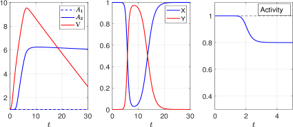
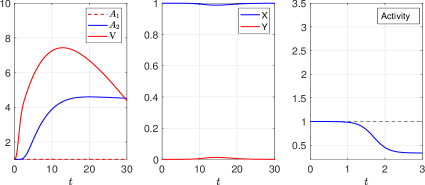
(b.1)                   (b.2)                   (b.3)                      (b^′.1)                   (b^′.2)                   (b^′.3)

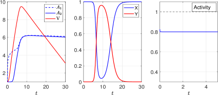
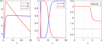
(c.1)                   (c.2)                   (c.3)                      (c^′.1)                   (c^′.2)                   (c^′.3)

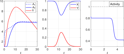
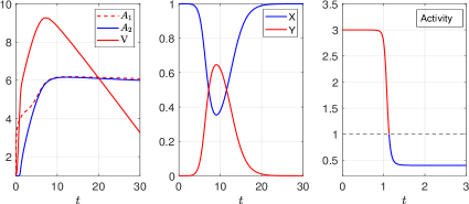
(d.1)                   (d.2)                   (d.3)                      (d^′.1)                   (d^′.2)                   (d^′.3)

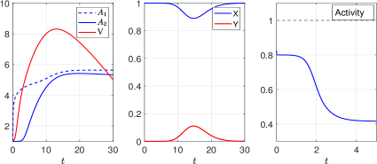
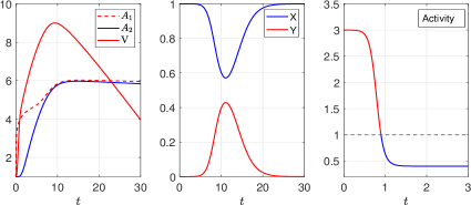
Figure 3: The first and third columns of the sub-figures, illustrate the temporal evolution of neutralizing (blue) or enhancing (red) antibody $A_{1}$ (dashed line), neutralizing antibody $A_{2}$ (blue solid line) and virus $V$ (red solid line). The second and fifth columns of the sub-figures show the evolution of susceptible and infected cells $X$ and $Y$ (blue and red solid line). The last two columns illustrate temporal virus activity (blue-red solid line).

6 Discussion

We developed a formula that gives the virus activity when bound to two antibodies, using the principle of chemical reactions. It generalizes the work of [11] by assuming that the antibodies can bind to multiple sites on a receptor. We have thus been able to show that this antigen-antibody complex can neutralize or enhance virus activity, given the interaction - competition or cooperation - between antibodies. The viral activity was then integrated into a model that emulates the interaction between healthy target cells, infected cells, viruses, and antibodies. This allows us to study the dynamic process of immune response when challenged by sequential homologous or heterologous viruses. We highlighted two scenarios: a mixture of two neutralizing antibodies and a mixture of enhancing and neutralizing antibodies. Other situations not considered in this study, such as the mixture of two types of enhancing antibodies, could be envisaged. This can happen, for example, when using therapeutic antibodies. In this case, $p_{i}$, $i=1,2$, can also be a function of time. We could also generalize the model to the case where there are more than two antibody types, as in polyclonal antibody therapy, but the number of parameters would increase rapidly, making parametrization, analysis, and interpretation of the model a challenge. By keeping the model as simple as possible, we were able to explore it analytically and numerically and assert that virus neutralization is associated with purely independent binding, while enhanced virus activity is expected when purely competitive binding occurs. This opens up promising modeling prospects for the study of second viral infections, vaccine efficacy, or antibody treatment. Other potential applications, such as transcriptional gene regulation, [5], or any field where there is an interaction between activation and inhibition processes, could be favored by this type of new modeling. If the condition (H3) and/or the assumption in Proposition 3 are relaxed, then we could have several endemic equilibrium points even in the parameter space where $\mathcal{R}_{0}<1$. It would be interesting to study their biological significance and asymptotic behavior, given that the latter depends on initial conditions such as the size of the virus inoculum and the amount of each antibody present in the mixture. Another challenge for our model is to be able to confront it with biological data for dengue, influenza, Covid-19, or HIV. This will be one of the objectives of our future work.

References

• [1] M. Adimy, P.F.A. Mancera, D.S. Rodrigues, F.L.P. Santos, and C.P. Ferreira, Maternal passive immunity and dengue hemorrhagic fever in infants, Bulletin of Mathematical Biology, 82, 24, (2020).
• [2] H. Ansari and M. Hesaaraki, A within-host dengue infection model with immune response and beddington-deangelis incidence rate, Applied Mathematics, 3(2), 177-184 (2012).
• [3] R. Ben-Shachar and K. Koelle, Minimal within-host dengue models highlight the specific roles of the immune response in primary and secondary dengue infections, Journal of the Royal Society Interface, 12, 103, (2015).
• [4] F.A. Camargo, M. Adimy, L. Esteva, C. Métayer, and C.P. Ferreira, Modeling the relationship between antibody-dependent enhancement and disease severity in secondary dengue infection, Bulletin of Mathematical Biology, 83(85), 1-28 (2021).
• [5] M. Cambón and Ó. Sánchez, Thermodynamic modelling of transcriptional control: a sensitivity analysis, Mathematics, 10(13), 1-18 (2022).
• [6] M. Cerón Gómez and H.M. Yang, A simple mathematical model to describe antibody-dependent enhancement in heterologous secondary infection in dengue, Mathematical Medicine and Biology: A Journal of the IMA, 36, 4, 411-438, (2018).
• [7] H.E. Clapham, V. Tricou, N. Van Vinh Chau, C.P. Simmons, and N. M. Ferguson, Within-host viral dynamics of dengue serotype 1 infection, Journal of the Royal Society Interface, 11, 96, 20140094, (2014).
• [8] H.E. Clapham, T.H. Quyen, D.T.H. Kien, I. Dorigatti, C.P. Simmons, and N.M. Ferguson, Modelling virus and antibody dynamics during dengue virus infection suggests a role for antibody in virus clearance, PLoS Computational Biology, 12(5), 1-15 (2016).
• [9] T. Dörner and A. Radbruch, Antibodies and B-cell memory in viral immunity, Immunity, 27(3), 384-392 (2007).
• [10] N.D. Durham, A. Agrawal, E. Waltari, D. Croote, F. Zanini, M. Fouch, E. Davidson, O. Smith, E. Carabajal, J.E. Pak, B.J. Doranz, M. Robinson, A.M. Sanz, L.L. Albornoz, F. Rosso, S. Einav, S.R. Quake, K.M. McCutcheon, and L. Goo, Broadly neutralizing human antibodies against dengue virus identified by single B-cell transcriptomics, ELife, 8, 1-29 (2019).
• [11] T. Einav and J.D. Bloom, When two are better than one: Modeling the mechanisms of antibody mixtures, PLoS Computational Biology, 16(5), 1-17 (2020).
• [12] C.F. Estofolete, A.F. Versiani, F.S. Dourado, B.H.G.A. Milhim, C.C. Pacca, G.C.D. Silva, N. Zini, B.F.D. Santos, F.A. Gandolfi, N.F.B. Mistrão, P.H.C. Garcia, R.S. Rocha, L. Gehrke, I. Bosch, R.E. Marques, M.M. Teixeira, F.G. da Fonseca, N. Vasilakis, and M.L. Nogueira, Influence of previous Zika virus infection on acute dengue episode, PLoS Neglected Tropical Diseases, 17(11), 1-25 (2023).
• [13] A.P. Goncalvez, R.E. Engle, M.St. Claire, R.H. Purcell, and C.-J. Lai, Monoclonal antibody-mediated enhancement of dengue virus infection in vitro and in vivo and strategies for prevention, Proceedings of The National Academy of Sciences, 104(22), 9422-9427 (2007).
• [14] T.P. Gujarati and G. Ambika, Virus antibody dynamics in primary and secondary dengue infections, Journal of Mathematical Biology, 69, 6, 1148-1155 (2014).
• [15] S.B. Halstead, Dengue Antibody-Dependent Enhancement: knowns and unknowns, Microbiology Spectrum, 2(6) (2014).
• [16] A.L.St. John and A.P.S. Rathore, Adaptive immune responses to primary and secondary dengue virus infections, Nature Reviews Immunology, 19, 218-230 (2019).
• [17] L.C. Katzelnick, L. Gresh, M.E. Halloran, J.C. Mercado, G. Kuan, A. Gordon, A. Balmaseda, and E. Harris, antibody-dependent enhancement of severe dengue disease in humans, Science, 358(6365), 929-932 (2017).
• [18] M. Kirkilionis and S. Walcher, On comparison systems for ordinary differential equations, Journal of Mathematical Analysis and Applications, 299(1), 157-173, (2004).
• [19] F. Klein, H. Mouquet, P. Dosenovic, J.F. Scheid, L. Scharf, and M.C. Nussenzweig, Antibodies in HIV-1 vaccine development and therapy, Science, 341(6151), 1199-1204 (2013).
• [20] T. Kuiken and J.K. Taubenberger, Pathology of human influenza revisited, Vaccine, 26(4), D59-D66 (2008).
• [21] J.L. Kyle, P.R. Beatty, and E. Harris, Dengue virus infects macrophages and dendritic cells in a mouse model of infection, The Journal of Infectious Diseases, 195(12), 1808-1817 (2007).
• [22] N. Nuraini, H. Tasman, E. Soewono, and K. A. Sidarto, A within-host dengue infection model with immune response, Mathematical and Computer Modelling, 49(5), 1148-1155 (2009).
• [23] P.W.H.I. Parren and D.R. Burton, The antiviral activity of antibodies in vitro and in vivo, Advances In Immunology, 77, 195-262 (2001).
• [24] K.A. Pawelek, G.T. Huynh, M. Quinlivan, A. Cullinane, L. Rong, and A.S. Perelson, Modeling within-host dynamics of influenza virus infection including immune responses, PLoS Computational Biology, 8, (2012).
• [25] A.S. Perelson and G. Weisbuch, Immunology for physicists, Reviews of Modern Physics, 69, 1219-1268 (1997).
• [26] A.S. Perelson, Modelling viral and immune system dynamics, Nature Reviews Immunology. 2, 28-36 (2002).
• [27] T.C. Pierson, D.H. Fremont, R.J. Kuhn, and M.S. Diamond, Structural insights into the mechanisms of antibody-mediated neutralization of flavivirus infection: implications for vaccine development, Cell Host and Microbe, 4, 229-238 (2008).
• [28] A. Puschnik, L. Lau, E.A. Cromwell, A. Balmaseda, S. Zompi, and E. Harris, Correlation between dengue-specific neutralizing antibodies and serum avidity in primary and secondary dengue virus 3 natural infections in humans, PLoS Neglected Tropical Diseases, 7(6), 1-8 (2013).
• [29] N.G. Reich, S. Shrestha, A.A. King, P. Rohani, J. Lessler, S. Kalayanarooj, I.-K. Yoon, R.V. Gibbons, D.S. Burke, and D.A.T. Cummings, Interactions between serotypes of dengue highlight epidemiological impact of cross-immunity, Journal of The Royal Society Interface, 10(86), 1-9 (2013).
• [30] I.A. Rodenhuis-Zybert, J. Wilschut, and J.M. Smit, Dengue virus life cycle: viral and host factors modulating infectivity, Cellular and Molecular Life Sciences, 67(16), 2773-2786 (2010).
• [31] T. Samji, Influenza A: understanding the viral life cycle, The Yale Journal of Biology and Medicine, 82(4), 153-159 (2009).
• [32] P.P. Sanna, F. Ramiro-Ibañez, and A. De Logu, Synergistic interactions of antibodies in rate of virus neutralization, Virology, 270(2), 386-396 (2000).
• [33] M. Santillán, On the use of the Hill functions in mathematical models of gene regulatory networks, Mathematical Modelling of Natural Phenomena, 3(2), 85-97 (2008).
• [34] A.M. Scott, J.D. Wolchok, and L.J. Old, Antibody therapy of cancer, Nature Reviews Cancer, 12, 278-287 (2012).
• [35] H. Smith, An Introduction to Delay Differential Equations with Applications to the Life Sciences, Springer New York, (2011).
• [36] H.L. Smith, P. Waltman, The Theory of the Chemostat, Cambridge University Press, Cambridge UK, (1995).
• [37] V. Tricou, N.N. Minh, J. Farrar, H.T. Tran, and C.P. Simmons, Kinetics of viremia and NS1 antigenemia are shaped by immune status and virus serotype in adults with dengue, PLoS Neglected Tropical Diseases. 5(9), 1-10 (2011).
• [38] V. Trouplin, N. Boucherit, L. Gorvel, F. Conti, G. Mottola, and E. Ghigo, Bone marrow-derived macrophage production, Journal of Visualized Experiments, 81: 50966 (2013).
• [39] P. Van den Driessche and J. Watmough, Reproduction numbers and sub-threshold endemic equilibria for compartmental models of disease transmission, Mathematical Biosciences, 180(1-2), 29-48 (2002).
• [40] J. Wen, Y. Cheng, R. Ling, Y. Dai, B. Huang, W. Huang, S. Zhang, Y. Jiang, Antibody-dependent enhancement of coronavirus, International Journal of Infectious Diseases, 100 483-489 (2020).
• [41] D. Wodarz, and M. Nowak, Mathematical models of HIV pathogenesis and treatment, BioEssays. 24, 1178-1187 (2002).
• [42] R. Xu, Global stability of an HIV-1 infection model with saturation infection and intracellular delay, Journal of Mathematical Analysis and Applications, 375(1), 75-81 (2011).