Pan-Mamba: Effective pan-sharpening with State Space Model

Abstract

Pan-sharpening involves integrating information from low-resolution multi-spectral and high-resolution panchromatic images to generate high-resolution multi-spectral counterparts. While recent advancements in the state space model, particularly the efficient long-range dependency modeling achieved by Mamba, have revolutionized computer vision community, its untapped potential in pan-sharpening motivates our exploration. Our contribution, Pan-Mamba, represents a novel pan-sharpening network that leverages the efficiency of the Mamba model in global information modeling. In Pan-Mamba, we customize two core components: channel swapping Mamba and cross-modal Mamba, strategically designed for efficient cross-modal information exchange and fusion. The former initiates a lightweight cross-modal interaction through the exchange of partial panchromatic and multispectral channels, while the latter facilities the information representation capability by exploiting inherent cross-modal relationships. Through extensive experiments across diverse datasets, our proposed approach surpasses state-of-the-art methods, showcasing superior fusion results in pan-sharpening. To the best of our knowledge, this work is the first attempt in exploring the potential of the Mamba model and establishes a new frontier in the pan-sharpening techniques. The source code is available at https://github.com/alexhe101/Pan-Mamba.

1 Introduction

In various domains such as agricultural monitoring and environmental protection, there exists a great need for high-resolution multispectral (HRMS) remote sensing image. However, owing to constraints imposed by physical laws and the associated hardware costs, acquiring high-resolution multispectral images directly through remote sensing satellites poses a considerable challenge. Typically, satellites are equipped with two distinct types of panchromatic and multispectral sensors, designed to capture low-resolution multispectral (LRMS) images and high-resolution texture-rich panchromatic (PAN) images. These two sets of images with complementary information are subsequently fused using a technique known as pan-sharpening, which enables the acquisition of high-resolution multispectral image.

Pan-sharpening technology has garnered considerable attention in recent years. Initial approaches relied on mathematical models for image fusion [15, 7]; however, manually designed models faced challenges due to inadequate representation, leading to suboptimal results. The pioneer PNN [18], inspired by SRCNN [4], which utilized three simple convolutional layers, marked a pivotal moment as it pioneered the integration of deep learning methods into this domain, showcasing great advancements over traditional techniques. Subsequently, a flood of increasingly complex models has been introduced, encompassing multi-scale methods [29], models leveraging frequency domain information [33, 12], architectures based on Transformer models [32, 31], models incorporating mixture of experts [11], and those driven by domain prior knowledge [26, 34].

Nevertheless, current methods exhibit certain limitations that hinder further improvement in performance. Firstly, challenges persist in capturing global information. INNformer [32] and Panformer [31] attempt to model global information by incorporating Vit [5] blocks and Swin Transformer blocks [17], respectively. However, the former introduces computational complexity, rendering its application challenging, while the latter’s window partitioning imposes constraints on the model’s receptive field and disrupts the locality of features [24]. SFINet [33] and MSDDN [12] adopt a different approach by introducing Fourier transform to model global information. However, the interaction between the frequency domain and spatial domain introduces information gaps [28], and the fixed convolution parameters hinder the model’s adaptive ability to varying inputs. Conversely, some techniques that aim to reduce the complexity of self-attention, such as window partitioning [17] and transposed self-attention [30], sacrifice to some extent the inherent capabilities of self-attention, including global information modeling and input adaptability. The birth of the Mamba [8] offers a novel solution to the aforementioned challenges. It features input-adaptive and global information modeling capabilities akin to self-attention, while maintaining linear complexity, reduced computational overhead, and enhanced inference speed. Notably, in the realm of natural language processing, the Mamba model has demonstrated superior results compared to the Transformer architecture.

Considering the aforementioned considerations, our approach focuses on enhancing models through two key perspectives: feature extraction and feature fusion. We introduce Pan-Mamba, a pan-sharpening network that leverages Mamba as the core module. Mamba is utilized for global information modeling, extracting global information from both PAN and LRMS images. Our design includes channel swapping Mamba and cross modal Mamba for efficient feature fusion. The channel swapping Mamba initiates a preliminary cross-modal interaction by exchanging partial pan channels and ms channels, facilitating a lightweight and efficient fusion of information. Meanwhile, the cross modal Mamba utilizes the inherent cross-modal relationship between the two, enabling fusion, filtering of redundant modal features, and obtaining refined fusion results. Owing to its efficient feature extraction and fusion capabilities, our model has surpassed state-of-the-art methods, achieving superior fusion results. Our contributions can be summarized as follows:

• We are the first to introduced the Mamba model into the pan-sharpening domain, presenting the Pan-Mamba model. This approach facilitates efficient long-range information modeling and cross-modal information interaction.

• We have designed channel swapping mamba block and cross modal mamba block for efficient cross modal information exchange and fusion.

• Through comprehensive experiments across multiple datasets, our proposed method demonstrated state-of-the-art results in both qualitative and quantitative assessments.

2 Related Work

2.1 Pan-sharpening

The methods of pan-sharpening is primarily categorized into two parts: traditional approaches and deep learning-based methods. Traditional methods predominantly rely on manually designed priors, encompassing component substitution algorithms [7, 15, 14, 10], multi-resolution analysis algorithms [21, 20], and variational optimization algorithms [6]. Component substitution algorithms leverage the spatial details of PAN images to replace the spatial information of LRMS images. Multi-resolution methods conduct multi-resolution analysis and subsequently fuse the two images, whereas variational optimization-based algorithms model the fusion process as an energy function and iteratively solve it. These methods suffer from limitations in performance due to their insufficient feature representation.

The rise of deep learning in pan-sharpening was initiated by the PNN [18] model, which, drawing inspiration from SRCNN [4], devised a simple three-layer neural network with promising outcomes. Subsequent advancements introduced more complex designs to this domain, such as PanNet [27] utilizing ResNet blocks to capture high-frequency information, MSDCNN [29] introducing multi-scale convolution for processing the multi-scale structure of remote sensing images, and SRPPNN [2] employing a progressive upsampling strategy. The emergence of Transformers has influenced pan-sharpening, with INNformers [32] and Panfomers [31] introducing self-attention mechanisms. SFINet [33] and MSDDN [12] employ Fourier transforms to capture global features and facilitate the learning of high-frequency information. Fame-Net [11] incorporates MOE structures for processing dynamic remote sensing images. Furthermore, prior information-driven methods have been integrated into this field, exemplified by MutNet [34] and GPPNN [26], which leverage prior knowledge between modalities to promote image fusion.

2.2 State Space Model

The concept of the State Space model was initially introduced in the S4 [9] model, presenting a distinctive architecture capable of effectively modeling global information in comparison to conventional CNN or Transformer architectures. Building upon S4, the S5 [22] model emerged, strategically reducing complexity to a linear level. The subsequent H3 [19] model further refined and expanded upon this foundation, enabling the model to perform competitively with Transformers in language model tasks. Mamba [8], in turn, introduced an input-adaptive mechanism to enhance the State Space model, resulting in higher inference speed, throughput, and overall metrics compared to Transformers of equivalent scale.

The application of the State Space model extended into visual tasks with the introduction of Vision Mamba [35] and Vmaba [16]. These adaptations yielded commendable results in classification and segmentation tasks, successfully penetrating fields such as medical image segmentation [25]. Notably, the potential of this model in multimodal image fusion remains an area that has not been thoroughly explored.

3 Methods

In this section, we begin by introducing the fundamental knowledge of the state space model. Subsequently, we delve into a detailed exploration of our model, encompassing its architectural framework, module design, and our loss function.

3.1 Preliminaries

The state space sequence model and Mamba draw inspiration from linear systems, with the goal of mapping a one-dimensional function or sequence, denoted as $x(t)\in\mathbf{R}$, to $y(t)$ through the hidden space $h(t)\in\mathbf{R}^{N}$. In this context, $\mathbf{A}\in\mathbf{R}^{N\times N}$ serves as the evolution parameter, while $\mathbf{B}\in\mathbf{R}^{N\times 1}$ and $\mathbf{C}\in\mathbf{R}^{1\times N}$ act as the projection parameters. The system can be mathematically expressed using the following formula.

$$h^{\prime}(t)=\mathbf{A}h(t)+\mathbf{B}x(t),$$ (1)

$$y(t)=\mathbf{C}h^{\prime}(t).$$ (2)

The S4 and Mamba models serve as discrete counterparts to the continuous system, incorporating a timescale parameter $\mathbf{\Delta}$ to convert continuous parameters $\mathbf{A}$ and $\mathbf{B}$ into their discrete counterparts $\bar{\mathbf{A}}$ and $\bar{\mathbf{B}}$. The prevalent approach employed for this transformation is the zero-order hold (ZOH) method, which can be formally defined as follows:

$$\bar{\mathbf{A}}=\mathbf{exp(\Delta A)},$$ (3)

$$\bar{\mathbf{B}}=\mathbf{(\Delta A)}^{-1}\mathbf{(exp(\Delta A)-I)\cdot\Delta B}.$$ (4)

The discrete representation of this linear system can be formulated as follows:

$$h_{t}=\bar{\mathbf{A}}h_{t-1}+\bar{\mathbf{B}}x_{t},$$ (5)

$$y_{t}=\mathbf{C}h_{t}.$$ (6)

Finally, the output is derived through global convolution:

$$\bar{\mathbf{K}}=(\mathbf{C\bar{B},C\bar{A}\bar{B},...,C\bar{A}^{M-1}\bar{B}}),$$ (7)

$$\mathbf{y}=x*\mathbf{\bar{K}}.$$ (8)

Here, $\mathbf{M}$ denotes the sequence length of x, and $\mathbf{\bar{K}}\in\mathbf{R}^{M}$ represents a structured convolutional kernel.

3.2 Network Architecture

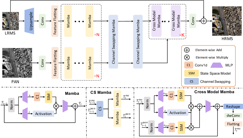
Figure 1: The network structure of our proposed Pan-Mamba, which includes three Key components: Mamba block for long-range feature extraction, EMamba and Cmamba for shallow and deep feature fusion.

The architecture of our model is depicted in Figure 1, comprising three core components: the Mamba block, the channel swapping Mamba block, and the cross modal Mamba block. The Mamba block is instrumental in modeling the long-range dependencies within PAN and LRMS features, while the channel swapping Mamba block and cross-modal Mamba block are employed to explore the relationship between the two modalities. Given the input LRMS and PAN images denoted as $M$ and $P$, the network pipeline can be expressed as follows:

Firstly, we employ convolutional layers to project the two images into the feature space and flatten them along the spatial dimension into tokens:

$$\mathbf{M}_{f},\mathbf{P}_{f}=\phi(\mathbf{M}),\phi(\mathbf{P}),$$ (9)

$$\mathbf{T}^{ms}_{0},\mathbf{T}^{pan}_{0}=\text{flatten}(\mathbf{M}_{f}),\text{flatten}(\mathbf{P}_{f}).$$ (10)

Subsequently, $\mathbf{T}^{ms}_{0}$ and $\mathbf{T}^{pan}_{0}$ are fed independently into a sequence of Mamba blocks for global feature extraction:

$$\mathbf{T}^{ms}_{i}=\psi_{m_{i}}..(\psi_{m_{1}}(\psi_{m_{0}}(\mathbf{T}^{ms}_{0}))),\ \mathbf{T}^{pan}_{i}=\psi_{p_{i}}..(\psi_{p_{1}}(\psi_{p_{0}}(\mathbf{T}^{pan}_{0}))).$$ (11)

Here, $\psi_{m_{i}}(.)$ and $\psi_{p_{i}}(.)$ denote the i-th Mamba block for extracting LRMS and PAN features, respectively.

Upon obtaining the global features $\mathbf{T}^{ms}_{i}$ and $\mathbf{T}^{pan}_{i}$, we leverage the channel swapping Mamba to enhance feature interaction and obtain $\mathbf{T}^{ms}_{k}$ and $\mathbf{T}^{pan}_{k}$. Subsequently, we utilize the cross modal Mamba block for deep feature fusion. After that, we reshape the MS token into the spatial dimension. The final output is obtained through convolution layers and residual connections:

$$\mathbf{T}^{ms}_{k+j}=\theta_{j}..(\theta_{1}(\theta_{0}(\mathbf{T}^{ms}_{k},\mathbf{T}^{pan}_{k}),\mathbf{T}^{pan}_{k}),\mathbf{T}^{pan}_{k}),$$ (12)

$$\mathbf{M}_{\text{out}}=\phi(\text{reshape}(\mathbf{T}^{ms}_{k+j}))+\mathbf{M}.$$ (13)

Here, $\theta(\cdot)$ represents the Cross Mamba block, and $\phi(\cdot)$ denotes the convolution layers for channel adjustment.

3.3 Key Components

3.3.1 Mamba Block

Motivated by the Mamba, we employ the Mamba block to extract features and model long-range dependencies. A comprehensive overview of the operations is provided in Algorithm 2. Specifically, the input token sequence $\mathbf{T}_{l-1}\in\mathbf{R^{B\times M\times D}}$ undergoes initial normalization via layer normalization. Subsequently, the normalized sequence is projected into $\mathbf{x}\in\mathbf{x^{B\times M\times E}}$ and $\mathbf{z}\in\mathbf{x^{B\times M\times E}}$ using a multi-layer perceptron (MLP). Following this, a 1-D convolution layer with SiLU activation is applied to process $\mathbf{x}$ and yield $\mathbf{x}^{\prime}$. Further projection of $\mathbf{x}^{\prime}$ onto $\mathbf{A}$, $\mathbf{B}$, and $\mathbf{C}$ is performed, and the timescale parameter $\mathbf{\Delta}$ is employed to convert them into discrete versions $\mathbf{\bar{A}}$ and $\mathbf{\bar{B}}$. The parameter generation process is delineated in Algorithm 1 and corresponds to formula 4. After that, the output $\mathbf{y}$ is computed through the SSM. Subsequently, $\mathbf{y}$ is gated by $\mathbf{z}$ and added to the input $\mathbf{T}_{l-1}$, to get the output sequence $\mathbf{T}_{l}$. The SSM process is describe in formula 8. The computational complexity of Mamba block exhibits linearity to the sequence length M. Specifically, the computational complexity is expressed as $3M(2D)N+M(2D)N$. Algorithm 1 Parameters Function 0:  token sequence $\mathbf{x}^{\prime}$ : $(\mathtt{B},\mathtt{M},\mathtt{E})$ 0:  token sequence $\mathbf{\bar{A}}$ : $(\mathtt{B},\mathtt{M},\mathtt{E},\mathtt{N})$,$\mathbf{\bar{B}}$ : $(\mathtt{B},\mathtt{M},\mathtt{E},\mathtt{N})$,$\mathbf{\bar{C}}$ : $(\mathtt{B},\mathtt{M},\mathtt{N})$ 1:  $\mathbf{B}$ : $(\mathtt{B},\mathtt{M},\mathtt{N})$ $\leftarrow$ $\mathbf{Linear}^{\mathbf{B}}(\mathbf{x}^{\prime})$ 2:  $\mathbf{C}$ : $(\mathtt{B},\mathtt{M},\mathtt{N})$ $\leftarrow$ $\mathbf{Linear}^{\mathbf{C}}(\mathbf{x}^{\prime})$ 3:  $\mathbf{\Delta}$ : $(\mathtt{B},\mathtt{M},\mathtt{E})$ $\leftarrow$ $\log(1+\exp(\mathbf{Linear}^{\mathbf{\Delta}}(\mathbf{x}^{\prime})+\mathbf{Parameter}^{\mathbf{\Delta}}))$ 4:  /* shape of $\mathbf{Parameter}^{\mathbf{A}}$ is $(\mathtt{E},\mathtt{N})$ */ 5:  $\overline{\mathbf{A}}$ : $(\mathtt{B},\mathtt{M},\mathtt{E},\mathtt{N})$ $\leftarrow$ $\mathbf{\Delta}_{o}\bigotimes\mathbf{Parameter}^{\mathbf{A}}$ 6:  $\overline{\mathbf{B}}$ : $(\mathtt{B},\mathtt{M},\mathtt{E},\mathtt{N})$ $\leftarrow$ $\mathbf{\Delta}_{o}\bigotimes\mathbf{B}$ Return: $\mathbf{\bar{A}},\mathbf{\bar{B}},\mathbf{C}$ Algorithm 2 Mamba Block 0:  token sequence $\mathbf{T}_{l-1}$ : $(\mathtt{B},\mathtt{M},\mathtt{D})$ 0:  token sequence $\mathbf{T}_{l}$ : $(\mathtt{B},\mathtt{M},\mathtt{D})$ 1:  /* normalize the input sequence $\mathbf{T}_{l-1}^{\prime}$ */ 2:  $\mathbf{T}_{l-1}^{\prime}$ : $(\mathtt{B},\mathtt{M},\mathtt{D})$ $\leftarrow$ $\mathbf{Norm}(\mathbf{T}_{l-1})$ 3:  $\mathbf{x}$ : $(\mathtt{B},\mathtt{M},\mathtt{E})$ $\leftarrow$ $\mathbf{Linear}^{\mathbf{x}}(\mathbf{T}_{l-1}^{\prime})$ 4:  $\mathbf{z}$ : $(\mathtt{B},\mathtt{M},\mathtt{E})$ $\leftarrow$ $\mathbf{Linear}^{\mathbf{z}}(\mathbf{T}_{l-1}^{\prime})$ 5:  /* process with sequence */ 6:  $\mathbf{x}^{\prime}$ : $(\mathtt{B},\mathtt{M},\mathtt{E})$ $\leftarrow$ $\mathbf{SiLU}(\mathbf{Conv1d}(\mathbf{x}))$ 7:  $\overline{\mathbf{A}}$:$(\mathtt{B},\mathtt{M},\mathtt{E},\mathtt{N})$ , $\overline{\mathbf{B}}$:$(\mathtt{B},\mathtt{M},\mathtt{E},\mathtt{N})$, $\mathbf{C}$ :$(\mathtt{B},\mathtt{M},\mathtt{N})$$\leftarrow$ $\mathbf{ParametersFunction}$($\mathbf{x}^{\prime}$) 8:  $\mathbf{y}$ : $(\mathtt{B},\mathtt{M},\mathtt{E})$ $\leftarrow$ $\mathbf{SSM}(\overline{\mathbf{A}},\overline{\mathbf{B}},\mathbf{C})(\mathbf{x}^{\prime})$ 9:  /* get gated $\mathbf{y}$ */ 10:  $\mathbf{y}^{\prime}$ : $(\mathtt{B},\mathtt{M},\mathtt{E})$ $\leftarrow$ $\mathbf{y}\bigodot\mathbf{SiLU}(\mathbf{z})$ 11:  /* residual connection */ 12:  $\mathbf{T}_{l}$ : $(\mathtt{B},\mathtt{M},\mathtt{D})$ $\leftarrow$ $\mathbf{Linear}^{\mathbf{T}}(\mathbf{y}^{\prime})+\mathbf{T}_{l-1}$ Return: $\mathbf{T}_{l}$

3.3.2 Channel Swapping Mamba Block

To encourage feature interaction between PAN and LRMS modalities and initiate a correlation between them, we introduced a Mamba fusion block based on channel swapping. This module efficiently swaps channels between LRMS and PAN features, facilitating lightweight feature interaction. The swapped features are then processed through the Mamba block. The channel swapping operation enhances cross-modal correlations by incorporating information from distinct channels, thereby enriching the diversity of channel features, which contributes to the overall improvement in model performance. Given LRMS features $\mathbf{T}^{ms}_{l-1}\in\mathbf{R}^{B,M,D}$ and PAN features $\mathbf{T}^{pan}_{l-1}\in\mathbf{R}^{B,M,D}$ as inputs, we split each feature along the channel dimension into two equal portions. The first half of channels from $\mathbf{T}^{ms}_{l-1}$ is concatenated with the latter half of $\mathbf{T}^{pan}_{l-1}$ and processed through the Mamba block for feature extraction. The obtained features are added to $\mathbf{T}^{ms}_{l-1}$, resulting in the creation of a new feature $\mathbf{T}^{ms}_{l}$. Simultaneously, the first half of $\mathbf{T}^{pan}_{l-1}$ is concatenated with the latter half of $\mathbf{T}^{ms}_{l-1}$ and passed through the Mamba block. The resulting features are added to $\mathbf{T}^{pan}_{l-1}$, generating $\mathbf{T}^{pan}_{l}$. These features encapsulate information from both modalities, enhancing overall feature diversity.

Algorithm 3 Cross Modal Mamba Block

0:  token sequence $\mathbf{T}^{ms}_{l-1}$ : $(\mathtt{B},\mathtt{M},\mathtt{D})$,$\mathbf{T}^{pan}_{l-1}$ : $(\mathtt{B},\mathtt{M},\mathtt{D})$

0:  token sequence $\mathbf{T}^{ms}_{l}$ : $(\mathtt{B},\mathtt{M},\mathtt{D})$

1:  for $o$ in {pan, ms} do

2:     /* normalize the input sequence $\mathbf{T}_{l-1}^{\prime}$ */

3:     $\mathbf{T{{}^{\prime}}}^{o}_{l-1}$ : $(\mathtt{B},\mathtt{M},\mathtt{D})$ $\leftarrow$ $\mathbf{Norm}(\mathbf{T}^{o}_{l-1})$

4:     $\mathbf{x}_{o}$ : $(\mathtt{B},\mathtt{M},\mathtt{E})$ $\leftarrow$ $\mathbf{Linear}^{\mathbf{x}}_{o}(\mathbf{T}^{o}_{l-1})$

5:     /* process with sequence */

6:     $\mathbf{x}^{\prime}_{o}$ : $(\mathtt{B},\mathtt{M},\mathtt{E})$ $\leftarrow$ $\mathbf{SiLU}(\mathbf{Conv1d}_{o}(\mathbf{x}_{o}))$

7:     $\overline{\mathbf{A}}_{o}$:$(\mathtt{B},\mathtt{M},\mathtt{E},\mathtt{N})$ , $\overline{\mathbf{B}}_{o}$:$(\mathtt{B},\mathtt{M},\mathtt{E},\mathtt{N})$, $\mathbf{C}_{o}$ :$(\mathtt{B},\mathtt{M},\mathtt{N})$$\leftarrow$ $\mathbf{ParametersFunction_{o}}$($\mathbf{x}^{\prime}_{o}$)

8:     $\mathbf{y}_{o}$ : $(\mathtt{B},\mathtt{M},\mathtt{E})$ $\leftarrow$ $\mathbf{SSM}(\overline{\mathbf{A}}_{o},\overline{\mathbf{B}}_{o},\mathbf{C}_{o})(\mathbf{x}^{\prime}_{o})$

9:  end for

10:  $\mathbf{z}$ : $(\mathtt{B},\mathtt{M},\mathtt{E})$ $\leftarrow$ $\mathbf{Linear}^{\mathbf{z}}(\mathbf{T{{}^{\prime}}}^{ms}_{l-1})$

11:  /* get gated $\mathbf{y}_{o}$ */

12:  $\mathbf{y}_{ms}^{\prime}$ : $(\mathtt{B},\mathtt{M},\mathtt{E})$ $\leftarrow$ $\mathbf{y}_{ms}\bigodot\mathbf{SiLU}(\mathbf{z})$

13:  $\mathbf{y}_{pan}^{\prime}$ : $(\mathtt{B},\mathtt{M},\mathtt{E})$ $\leftarrow$ $\mathbf{y}_{pan}\bigodot\mathbf{SiLU}(\mathbf{z})$

14:  /* residual connection */

15:  $\mathbf{F}^{ms}_{l-1}$ : $(\mathtt{B},\mathtt{D},\mathtt{H},\mathtt{W})$ $\leftarrow$ $\mathbf{Reshape(\mathbf{Linear}^{\mathbf{T}}(\mathbf{y}_{ms}^{\prime}+\mathbf{y}_{pan}^{\prime})+\mathbf{T}^{ms}_{l-1})}$

16:  /* depth-wise convolution */

17:  $\mathbf{T}^{ms}_{l}$: $(\mathtt{B},\mathtt{M},\mathtt{D})$ $\leftarrow$ $\mathbf{Flatten}(\mathbf{DWConv}(\mathbf{F}^{ms}_{l-1})+\mathbf{F}^{ms}_{l-1})$ Return: $\mathbf{T}^{ms}_{l}$

3.3.3 Cross modality Mamba Block

Motivated by the concept of Cross Attention [3], we introduce a novel cross modal Mamba block designed for facilitating cross-modal feature interaction and fusion. In this approach, we project features from two modalities into a shared space, employing gating mechanisms to encourage complementary feature learning while suppressing redundant features. Concurrently, to enhance local features, we incorporate depth-wise convolution within the module, thereby amplifying the encoding capacity of local features during the fusion process. The details of this module are elucidated in Algo 3. The generation of $y_{ms}$ and $y_{pan}$ follows the process outlined in the Mamba block. Subsequently, we obtain the gating parameters $z$ by projecting $\mathbf{T{{}^{\prime}}}^{ms}_{l-1}$ and employ $z$ to modulate $y{ms}$ and $y_{pan}$. The fusion of these two features involves addition, followed by reshaping to obtain a 2-D feature $\mathbf{F}^{ms}_{l-1}$. To enhance locality, we apply depth-wise convolution, and subsequently flatten the feature to a 1-D sequence, generating output sequence $\mathbf{T}^{ms}_{l}$.

3.4 Loss Function

In alignment with the prevalent practices in this filed, we adopt the L1 loss as our chosen loss function. Specifically, with the output denoted as $\mathbf{M_{out}}$ and the corresponding ground truth as $\mathbf{G}$, the loss function is expressed as:

$$\mathcal{L}=||\mathbf{G}-\mathbf{M_{out}}||_{1}$$ (14)

4 Experiment

4.1 Datasets and Benchmark

In our experiments, we selected datasets comprising WorldView-II and WorldView-III, characterized by diverse resolutions and a broad spectrum of scenes. Specifically, WorldView-II encompasses industrial areas and natural landscapes, while WorldView-III predominantly features urban roads and urban scenes. Given the absence of ground truth, the dataset generating process adheres to the Wald protocol [23]. For comparative analysis, we opted for a selection of representative traditional methods, including GFPCA [14], GS [13], Brovey [7], IHS [10], and SFIM [15], alongside advanced deep learning methods such as PanNet [27], msdcnn [29], srppnn [2], INNformer [32], SFINet [33], MSDDN [12], and FAME-Net [11]. The chosen evaluation metrics encompass PSNR, SSIM, SAM (spectral angle mapper) [sam], and ERGAS (relative global error in synthesis) [1].

4.2 Implement Details

Utilizing the PyTorch framework, our code implementation and training procedures are executed on an Nvidia V100 GPU. The model features are configured with N=32 channels.

We initialize the learning rate at 5e-4, employing a cosine decay scheduling strategy. After 500 epochs, the learning rate diminishes to 5e-8. Optimization is carried out using the Adam optimizer, with gradient clipping set to 4 for training stability. Given variations in data sizes, we set the number of training epochs to 200 for the WorldView-II dataset and 500 for the WorldView-III dataset.

4.3 Comparison with State of Arts Methods

Table 1: Quantitative comparison on three datasets. Best results highlighted in red. $\uparrow$ indicates that the larger the value, the better the performance, and $\downarrow$ indicates that the smaller the value, the better the performance.

	WorldView-II				WorldView-III				Params(M)	FLOPS(G)
Method	PSNR$\uparrow$	SSIM$\uparrow$	SAM$\downarrow$	ERGAS$\downarrow$	PSNR$\uparrow$	SSIM$\uparrow$	SAM$\downarrow$	ERGAS$\downarrow$	-	-
SFIM	34.1297	0.8975	0.0439	2.3449	21.8212	0.5457	0.1208	8.9730	-	-
Brovey	35.8646	0.9216	0.0403	1.8238	22.5060	0.5466	0.1159	8.2331	-	-
IHS	35.6376	0.9176	0.0423	1.8774	22.5608	0.5470	0.1217	8.2433	-	-
GS	35.2962	0.9027	0.0461	2.0278	22.5579	0.5354	0.1266	8.3616	-	-
GFPCA	34.5581	0.9038	0.0488	2.1411	22.3344	0.4826	0.1294	8.3964	-	-
PanNet	40.8176	0.9626	0.0257	1.0557	29.6840	0.9072	0.0851	3.4263	0.0688	1.1275
MSDCNN	41.3355	0.9664	0.0242	0.9940	30.3038	0.9184	0.0782	3.1884	0.2390	3.9158
SRPPNN	41.4538	0.9679	0.0233	0.9899	30.4346	0.9202	0.0770	3.1553	1.7114	21.1059
INNformer	41.6903	0.9704	0.0227	0.9514	30.5365	0.9225	0.0747	3.099	0.0706	1.3079
SFINet	41.7244	0.9725	0.0220	0.9506	30.5901	0.9236	0.0741	3.0798	0.0871	1.2558
MSDDN	41.8435	0.9711	0.0222	0.9478	30.8645	0.9258	0.0757	2.9581	0.3185	2.5085
FAME-Net	42.0262	0.9723	0.0215	0.9172	30.9903	0.9287	0.0697	2.9531	0.1734	2.8225
Ours	42.2354	0.9729	0.0212	0.8975	31.1551	0.9299	0.0702	2.8942	0.1827	3.0088

4.3.1 Quantitative Comparison

In our comparative analysis depicted in Table 1, we benchmarked our proposed method against state-of-the-art techniques in the field. The results highlight significant improvement achieved by our proposed network structure, outperforming other methods across various evaluation metrics. Notably, on both the WorldView-II and WorldView-III datasets, our method demonstrated noteworthy improvements in PSNR metrics, with enhancements of 0.21 and 0.16, respectively. This indicates a closer alignment of our results with the ground truth. Similar trends are observed in the SSIM indicator, while the SAM indicator signifies spectral similarity. Our spectral similarity on WV2 surpasses state-of-the-art methods, with comparable outcomes on the WV3 dataset. The ERGAS indicator validate the overall superior performance of our method across each spectral band, substantiating its efficacy.

4.3.2 Qualitative Comparison

Quantitative results of the model are illustrated in Figures 2 and 3. Representative samples were chosen for visualization, and the last row of each image depicts the mean square error map of the pan-sharpened result in comparison to the ground truth. Brighter regions indicate greater discrepancies. Our method consistently yields the smallest errors, underscoring its proximity to the ground truth. Furthermore, upon pan-sharpened the results, our method exhibits superior performance in extracting high-frequency information and preserving spectral details, leading to clearer texture.

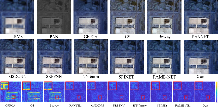
Figure 2: The result of our approach was compared against nine other methods on WorldView-II dataset.

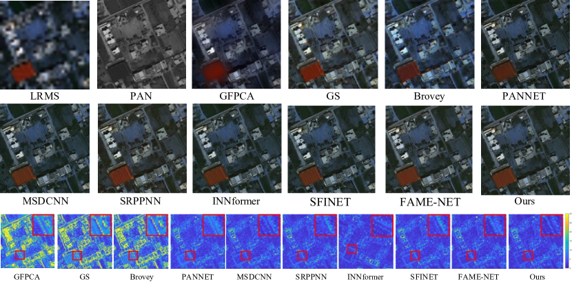
Figure 3: The result of our approach was compared against nine other methods on WorldView-III dataset.

Table 2: Ablation for Pan-Mamba on Worldview-II datasets. The PSNR/SSIM/SAM/ERGAS values on benchmarks are reported. "A → B" is to replace A with B. "None" The numbers of parameters, #FLOPs are counted by the fvcore library with a resolution of 128 × 128 pixels. Best results are highlighted in red.

Ablation	Variant	#Params [M]	#FLOPs [G]	WorldView-II
Baseline	-	0.1827	3.0028	42.2354/0.9729/0.0212/0.8975
Main module	Mamba Block->Conv3x3	0.3307	5.4248	42.1659/0.9725/0.0211/0.8979
	Channel Swapping Mamba->None	0.1827	3.0008	42.2294/0.9727/0.0212/0.8972
	Cross modal Mamba->None	0.1811	2.9852	42.0733/0.9716/0.0215/0.9109

4.4 Ablation Study

To comprehensively assess the contribution of each module, we conducted ablation experiments. To ensure fairness in comparison, we conducted training and reported experimental results exclusively on the WorldView-II dataset, maintaining consistent experimental configurations across all ablation experiments. The three core modules proposed in our paper were systematically examined in separate ablation experiment sets. Each set involved the removal or replacement of a specific module, allowing us to verify the overall performance impact of each component on the network.

4.4.1 Effectiveness of the Mamba Block

Our first set of ablation experiment is devised to validate the efficacy of the Mamba block in feature extraction. Within our model, the Mamba block plays a crucial role in modeling long-range dependencies in features. In this set of experiments, we substituted the Mamba block with a standard $3\times 3$ convolution operation and relocated the flattening operation in the model post feature extraction. The results from the second row of table 2 reveal a decline in model performance when the Mamba block is removed, providing evidence of the block’s effectiveness.

4.4.2 Effectiveness of the Channel Swapping Mamba Block

Our second set of ablation experiments is designed to validate the effectiveness of the Channel Swapping Mamba. Within our architecture, the Channel Swapping Mamba is specifically designed for shadow feature fusion, enhancing the diversity of channel features. In this experiment, we eliminated the channel swapping operation along with its associated Mamba block. As shown in the third row of table 2, despite the low computational cost of this module, the removal resulted in a noticeable decline in performance, underscoring the efficacy of this module.

4.4.3 Effectiveness of the Cross Modal Mamba Block

The third set of ablation experiments is conducted to substantiate the effectiveness of our pivotal fusion module, the cross-modal Mamba block. This module is designed to conduct deep fusion on LRMS and Pan features, reducing redundant features through gating mechanisms. In this experiment, we directly remove the cross modal Mamba block and exclusively employed the Channel Swapping Mamba for feature fusion. The results depicted in the table 2 showcase a substantial decline in the model’s performance following the removal of the Cross-Modal Mamba block.

5 Conclusion

In this study, drawing inspiration from the State Space model, we introduce a novel Pan-sharpening network, termed Pan Mamba. This innovative network incorporates Mamba blocks, Channel Swapping Mamba blocks, and Cross-Modal Mamba blocks. The proposed network achieves efficient global feature extraction and facilitates cross-modal information exchange with linear complexity. Notably, it outperforms state-of-the-art methods with a lightweight model on publicly available remote sensing datasets, showcasing robust spectral accuracy and adept preservation of texture information.

References

- [1] Alparone, L., Wald, L., Chanussot, J., Thomas, C., Gamba, P., Bruce, L.M.: Comparison of pansharpening algorithms: Outcome of the 2006 grs-s data fusion contest. IEEE Transactions on Geoscience and Remote Sensing 45(10), 3012–3021 (2007)
- [2] Cai, J., Huang, B.: Super-resolution-guided progressive pansharpening based on a deep convolutional neural network. IEEE Transactions on Geoscience and Remote Sensing 59(6), 5206–5220 (2021). https://doi.org/10.1109/TGRS.2020.3015878
- [3] Chen, C.F.R., Fan, Q., Panda, R.: Crossvit: Cross-attention multi-scale vision transformer for image classification. In: Proceedings of the IEEE/CVF international conference on computer vision. pp. 357–366 (2021)
- [4] Dong, C., Loy, C.C., He, K., Tang, X.: Image super-resolution using deep convolutional networks. IEEE Transactions on Pattern Analysis and Machine Intelligence 38(2), 295–307 (2016). https://doi.org/10.1109/TPAMI.2015.2439281
- [5] Dosovitskiy, A., Beyer, L., Kolesnikov, A., Weissenborn, D., Zhai, X., Unterthiner, T., Dehghani, M., Minderer, M., Heigold, G., Gelly, S., et al.: An image is worth 16x16 words: Transformers for image recognition at scale. arXiv preprint arXiv:2010.11929 (2020)
- [6] Fasbender, D., Radoux, J., Bogaert, P.: Bayesian data fusion for adaptable image pansharpening. IEEE Transactions on Geoscience and Remote Sensing 46(6), 1847–1857 (2008)
- [7] Gillespie, A.R., Kahle, A.B., Walker, R.E.: Color enhancement of highly correlated images. ii. channel ratio and "chromaticity" transformation techniques - sciencedirect. Remote Sensing of Environment 22(3), 343–365 (1987)
- [8] Gu, A., Dao, T.: Mamba: Linear-time sequence modeling with selective state spaces. arXiv preprint arXiv:2312.00752 (2023)
- [9] Gu, A., Goel, K., Ré, C.: Efficiently modeling long sequences with structured state spaces. arXiv preprint arXiv:2111.00396 (2021)
- [10] Haydn, R., Dalke, G.W., Henkel, J., Bare, J.E.: Application of the ihs color transform to the processing of multisensor data and image enhancement. National Academy of Sciences of the United States of America 79(13), 571–577 (1982)
- [11] He, X., Yan, K., Li, R., Xie, C., Zhang, J., Zhou, M.: Frequency-adaptive pan-sharpening with mixture of experts. arXiv preprint arXiv:2401.02151 (2024)
- [12] He, X., Yan, K., Zhang, J., Li, R., Xie, C., Zhou, M., Hong, D.: Multi-scale dual-domain guidance network for pan-sharpening. IEEE Transactions on Geoscience and Remote Sensing (2023)
- [13] Laben, C., Brower, B.: Process for enhancing the spatial resolution of multispectral imagery using pan-sharpening. US Patent 6011875A (2000)
- [14] Liao, W., Xin, H., Coillie, F.V., Thoonen, G., Philips, W.: Two-stage fusion of thermal hyperspectral and visible rgb image by pca and guided filter. In: Workshop on Hyperspectral Image and Signal Processing: Evolution in Remote Sensing (2017)
- [15] Liu., J.G.: Smoothing filter-based intensity modulation: A spectral preserve image fusion technique for improving spatial details. International Journal of Remote Sensing 21(18), 3461–3472 (2000)
- [16] Liu, Y., Tian, Y., Zhao, Y., Yu, H., Xie, L., Wang, Y., Ye, Q., Liu, Y.: Vmamba: Visual state space model. arXiv preprint arXiv:2401.10166 (2024)
- [17] Liu, Z., Lin, Y., Cao, Y., Hu, H., Wei, Y., Zhang, Z., Lin, S., Guo, B.: Swin transformer: Hierarchical vision transformer using shifted windows. In: Proceedings of the IEEE/CVF international conference on computer vision. pp. 10012–10022 (2021)
- [18] Masi, G., Cozzolino, D., Verdoliva, L., Scarpa, G.: Pansharpening by convolutional neural networks. Remote Sensing 8(7), 594 (2016)
- [19] Mehta, H., Gupta, A., Cutkosky, A., Neyshabur, B.: Long range language modeling via gated state spaces. arXiv preprint arXiv:2206.13947 (2022)
- [20] Nunez, J., Otazu, X., Fors, O., Prades, A., Pala, V., Arbiol, R.: Multiresolution-based image fusion with additive wavelet decomposition. IEEE Transactions on Geoscience and Remote sensing 37(3), 1204–1211 (1999)
- [21] Schowengerdt, R.A.: Reconstruction of multispatial, multispectral image data using spatial frequency content. Photogrammetric Engineering and Remote Sensing 46(10), 1325–1334 (1980)
- [22] Smith, J.T., Warrington, A., Linderman, S.W.: Simplified state space layers for sequence modeling. arXiv preprint arXiv:2208.04933 (2022)
- [23] Wald, L., Ranchin, T., Mangolini, M.: Fusion of satellite images of different spatial resolutions: Assessing the quality of resulting images. Photogrammetric Engineering and Remote Sensing 63, 691–699 (11 1997)
- [24] Xiao, J., Fu, X., Zhou, M., Liu, H., Zha, Z.J.: Random shuffle transformer for image restoration. In: International Conference on Machine Learning. pp. 38039–38058. PMLR (2023)
- [25] Xing, Z., Ye, T., Yang, Y., Liu, G., Zhu, L.: Segmamba: Long-range sequential modeling mamba for 3d medical image segmentation. arXiv preprint arXiv:2401.13560 (2024)
- [26] Xu, S., Zhang, J., Zhao, Z., Sun, K., Liu, J., Zhang, C.: Deep gradient projection networks for pan-sharpening. In: IEEE Conference on Computer Vision and Pattern Recognition. pp. 1366–1375 (June 2021)
- [27] Yang, J., Fu, X., Hu, Y., Huang, Y., Ding, X., Paisley, J.: Pannet: A deep network architecture for pan-sharpening. In: IEEE International Conference on Computer Vision. pp. 5449–5457 (2017)
- [28] Yu, H., Huang, J., Li, L., Zhao, F., et al.: Deep fractional fourier transform. Advances in Neural Information Processing Systems 36 (2024)
- [29] Yuan, Q., Wei, Y., Meng, X., Shen, H., Zhang, L.: A multiscale and multidepth convolutional neural network for remote sensing imagery pan-sharpening. IEEE Journal of Selected Topics in Applied Earth Observations and Remote Sensing 11(3), 978–989 (2018)
- [30] Zamir, S.W., Arora, A., Khan, S., Hayat, M., Khan, F.S., Yang, M.H.: Restormer: Efficient transformer for high-resolution image restoration. In: Proceedings of the IEEE/CVF conference on computer vision and pattern recognition. pp. 5728–5739 (2022)
- [31] Zhou, H., Liu, Q., Wang, Y.: Panformer: A transformer based model for pan-sharpening. In: 2022 IEEE International Conference on Multimedia and Expo (ICME). pp. 1–6. IEEE (2022)
- [32] Zhou, M., Huang, J., Fang, Y., Fu, X., Liu, A.: Pan-sharpening with customized transformer and invertible neural network. In: Proceedings of the AAAI Conference on Artificial Intelligence. vol. 36, pp. 3553–3561 (2022)
- [33] Zhou, M., Huang, J., Yan, K., Yu, H., Fu, X., Liu, A., Wei, X., Zhao, F.: Spatial-frequency domain information integration for pan-sharpening. In: European Conference on Computer Vision. pp. 274–291. Springer (2022)
- [34] Zhou, M., Yan, K., Huang, J., Yang, Z., Fu, X., Zhao, F.: Mutual information-driven pan-sharpening. In: Proceedings of the IEEE/CVF Conference on Computer Vision and Pattern Recognition. pp. 1798–1808 (2022)
- [35] Zhu, L., Liao, B., Zhang, Q., Wang, X., Liu, W., Wang, X.: Vision mamba: Efficient visual representation learning with bidirectional state space model. arXiv preprint arXiv:2401.09417 (2024)